© 2001 ComputerPREP, Inc. All rights reserved.

Excel 2003 Expert

© 2001 ComputerPREP, Inc. All rights reserved.

Lesson 1:Organizing and Analyzing Data

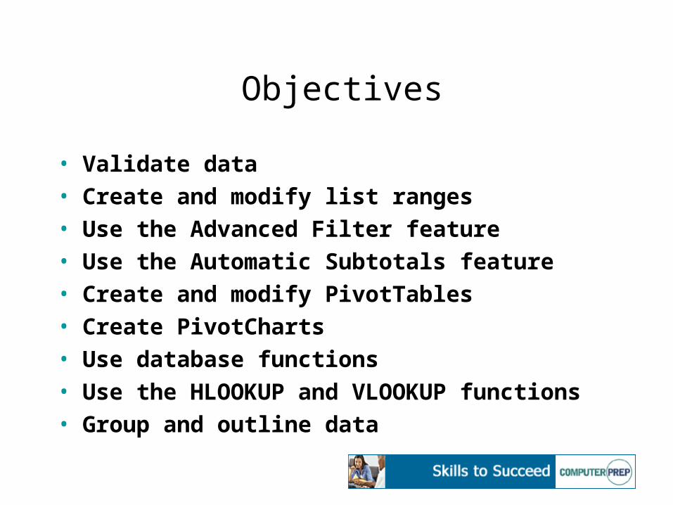
Objectives

• Validate data• Create and modify list ranges• Use the Advanced Filter feature• Use the Automatic Subtotals feature• Create and modify PivotTables• Create PivotCharts• Use database functions• Use the HLOOKUP and VLOOKUP functions• Group and outline data

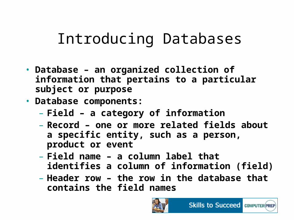
Introducing Databases

• Database – an organized collection of information that pertains to a particular subject or purpose

• Database components:– Field – a category of information– Record – one or more related fields about a

specific entity, such as a person, product or event

– Field name – a column label that identifies a column of information (field)

– Header row – the row in the database that contains the field names

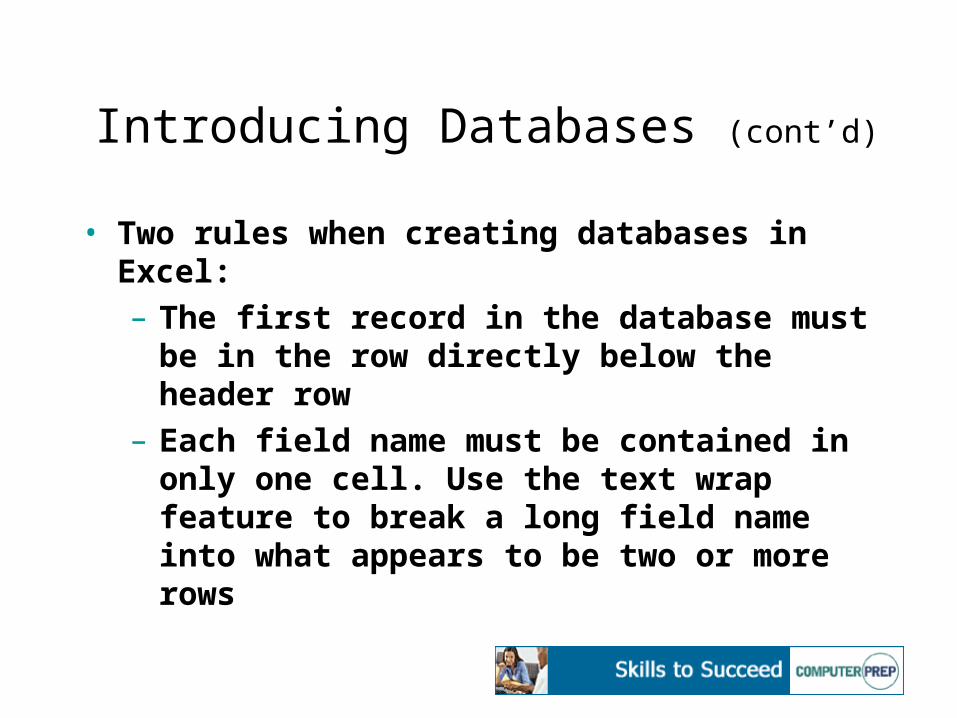
Introducing Databases (cont’d)

• Two rules when creating databases in Excel:– The first record in the database must be in the

row directly below the header row– Each field name must be contained in only one

cell. Use the text wrap feature to break a long field name into what appears to be two or more rows

Validating Data

• Use data validation to specify permissible data for specific fields– Data validation – restricts database entries to

specific text, whole numbers, decimal numbers, dates or any other set of criteria you specify

Creating and Modifying List Ranges

• List range – a feature that enables you to apply database functionality to a group of related data in a specified range

• You can manage and analyze the data in the list independently of data outside the list

• You can create as many list ranges in your worksheet as you want

Creating and Modifying List Ranges (cont’d)

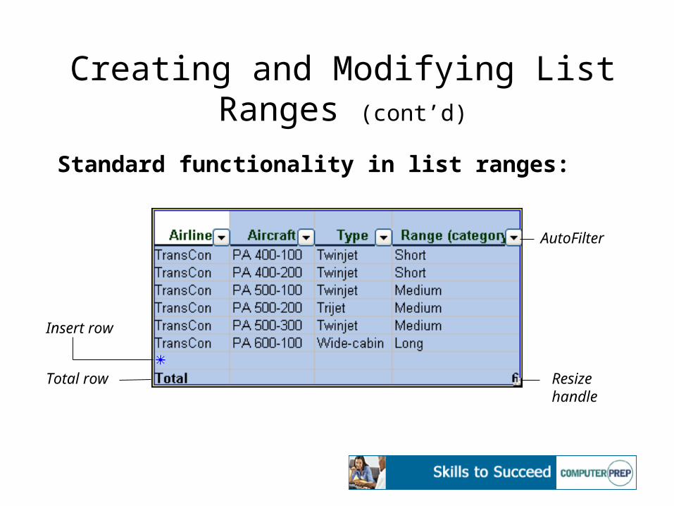
Standard functionality in list ranges:

Insert row

Total row

AutoFilter

Resize handle

Using the Advanced Filter Feature

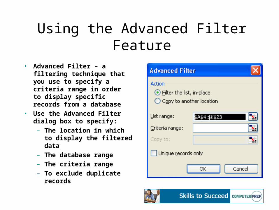
• Advanced Filter – a filtering technique that you use to specify a criteria range in order to display specific records from a database

• Use the Advanced Filter dialog box to specify:

– The location in which to display the filtered data

– The database range

– The criteria range

– To exclude duplicate records

Inserting Automatic Subtotals

• Automatic Subtotals – a feature that summarizes data in a database by grouping and performing specific calculations on the data

• Organize the data so that the records you want to subtotal are grouped together

• Use the Subtotal dialog box to:– Specify the field you want to summarize– Specify the function to use in calculating subtotals– Specify the fields containing the values you want to

subtotal– Place the subtotal and grand total rows above or below

the detail data

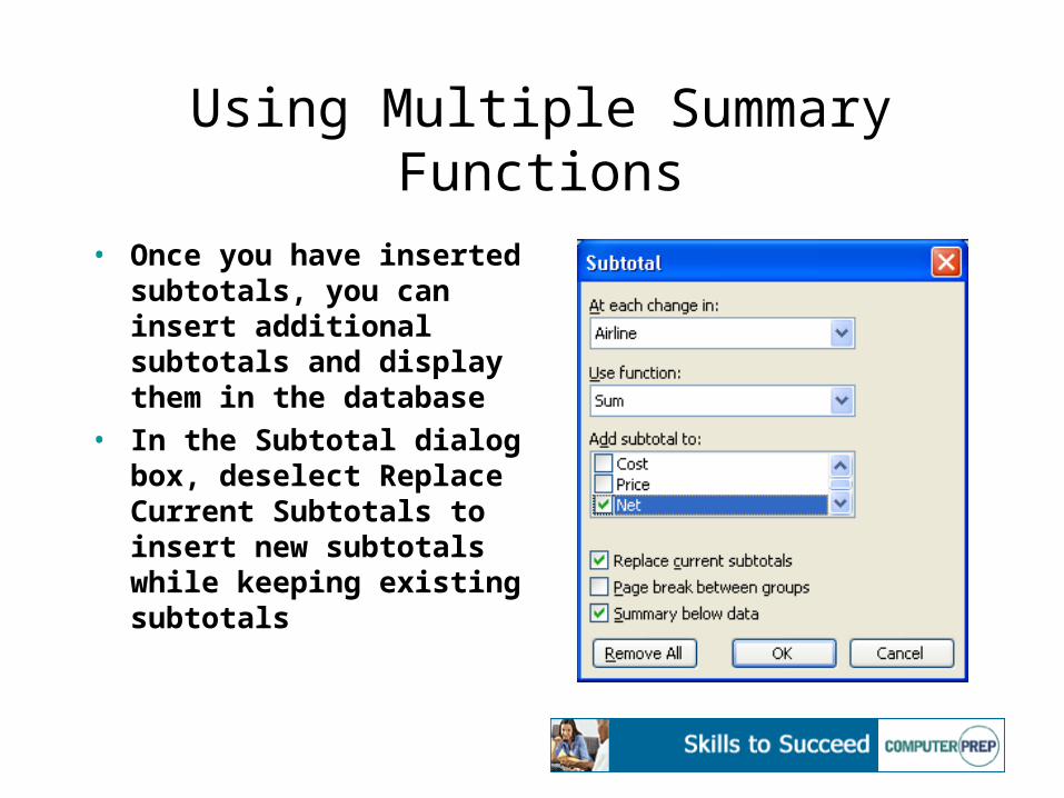
Using Multiple Summary Functions

• Once you have inserted subtotals, you can insert additional subtotals and display them in the database

• In the Subtotal dialog box, deselect Replace Current Subtotals to insert new subtotals while keeping existing subtotals

Hiding and Displaying Record Detail

• When you insert automatic subtotals, outline symbols display to the left of the worksheet window

• Use the row level symbols or the plus and minus signs to hide or display the level of record detail you want

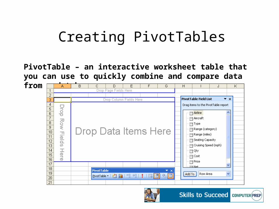
Creating PivotTables

PivotTable – an interactive worksheet table that you can use to quickly combine and compare data from a database

Modifying PivotTables

• Modify a PivotTable by:– Dragging field buttons to different sections of

the PivotTable to rearrange the data display– Adding field buttons from the PivotTable Field

List to the PivotTable– Removing field buttons from the PivotTable– Hiding and displaying data items for specific

fields in the PivotTable

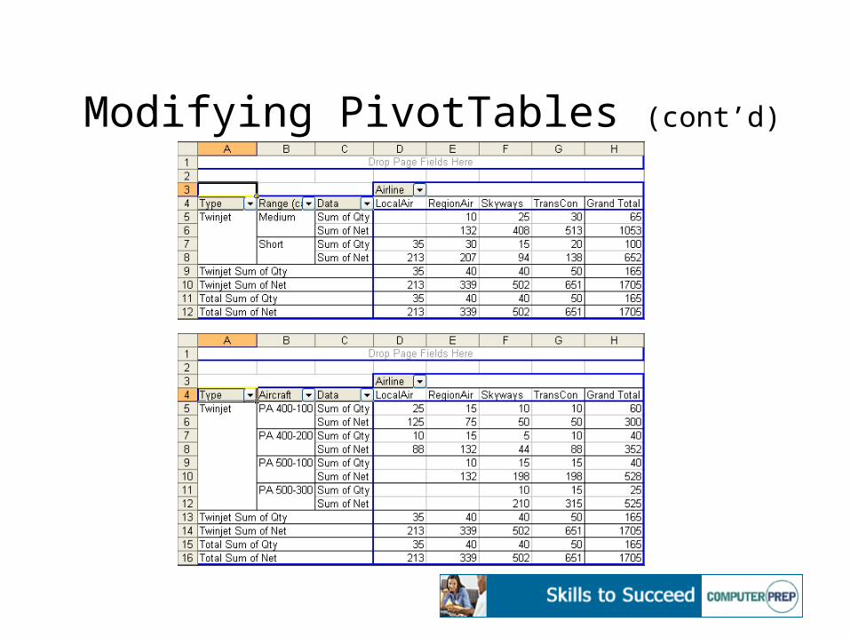
Modifying PivotTables (cont’d)

Creating PivotCharts

• PivotChart – provides a graphical representation of the data in a PivotTable

• The PivotChart and its associated PivotTable are interrelated; any change you make to one is automatically reflected in the other

About Database Functions• Database function – a built-in function that

calculates a value that is determined by the function type, the database field you specify, and the criteria you use to screen field values

• Database functions contain three arguments:– Database – the worksheet range that defines the

database– Field – the database field containing the values

to be used in the calculation– Criteria – the criteria range containing the

condition(s) you set to screen field values

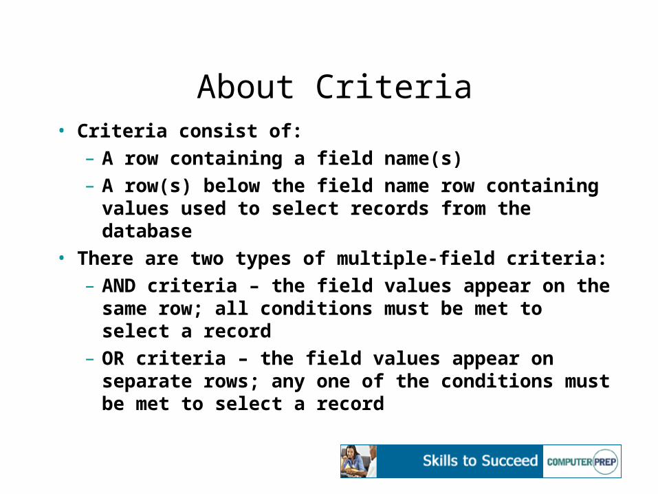
About Criteria• Criteria consist of:

– A row containing a field name(s)– A row(s) below the field name row containing

values used to select records from the database• There are two types of multiple-field criteria:

– AND criteria – the field values appear on the same row; all conditions must be met to select a record

– OR criteria – the field values appear on separate rows; any one of the conditions must be met to select a record

The DAVERAGE and DSUM Functions

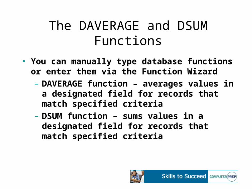
• You can manually type database functions or enter them via the Function Wizard– DAVERAGE function – averages values in a

designated field for records that match specified criteria

– DSUM function – sums values in a designated field for records that match specified criteria

The HLOOKUP and VLOOKUP Functions

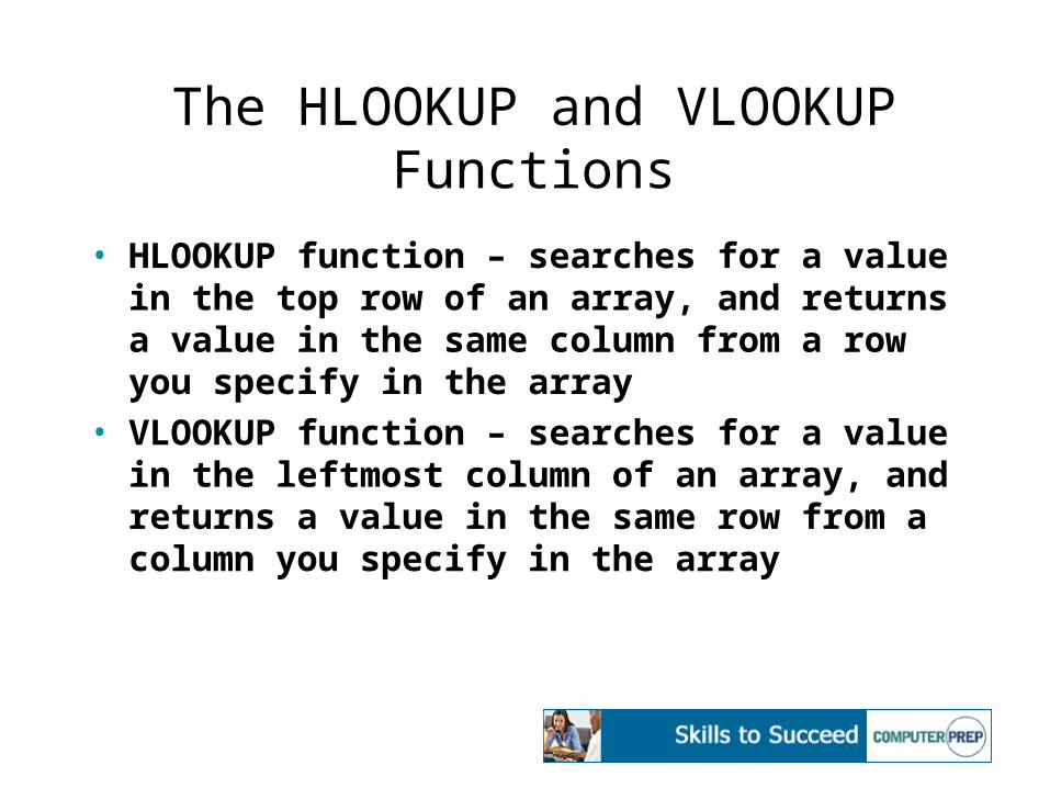
• HLOOKUP function – searches for a value in the top row of an array, and returns a value in the same column from a row you specify in the array

• VLOOKUP function – searches for a value in the leftmost column of an array, and returns a value in the same row from a column you specify in the array

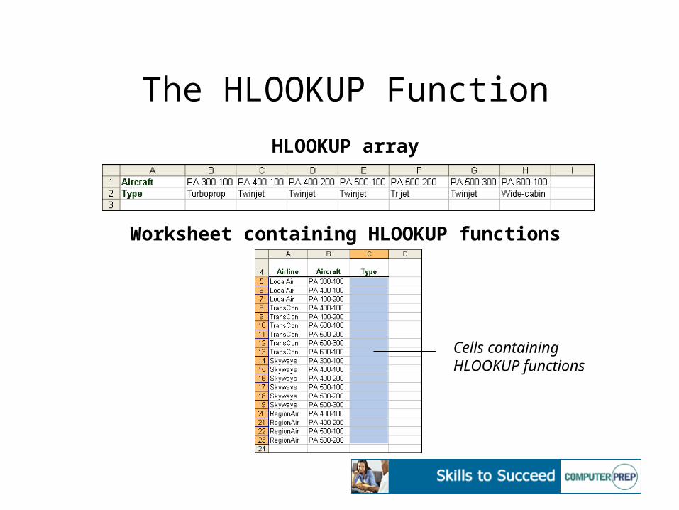
The HLOOKUP Function

HLOOKUP array

Worksheet containing HLOOKUP functions

Cells containingHLOOKUP functions

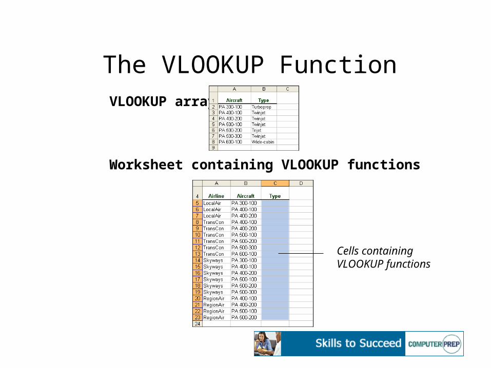
The VLOOKUP FunctionVLOOKUP array

Worksheet containing VLOOKUP functions

Cells containingVLOOKUP functions

Grouping and Outlining Data

• Group – manually outlines rows or columns of worksheet data

• Outline – categorizes rows or columns of worksheet entries as detail data or various levels of summary data

• Summary data – rows or columns containing formulas that summarize detail data

Grouping and Outlining Data (cont’d)

• Group data when you want to outline a worksheet that does not contain summary data

• Automatically outline data when you want to outline a worksheet that contains summary data

• The summary data must be adjacent to the detail data

• Outline symbols display to the left of or on top of the worksheet

• Click outline symbols to hide or display various levels of detail

© 2001 ComputerPREP, Inc. All rights reserved.

Lesson 2:Auditing Worksheets and

Performing What-If Analyses

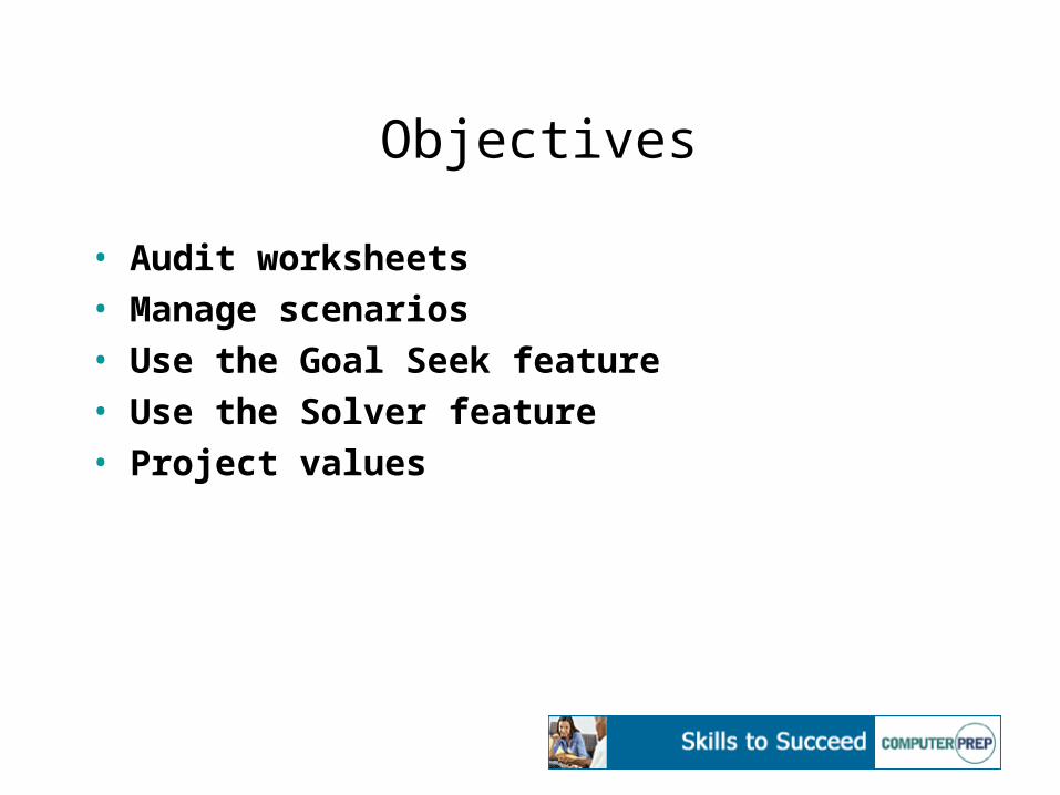
Objectives

• Audit worksheets• Manage scenarios• Use the Goal Seek feature• Use the Solver feature• Project values

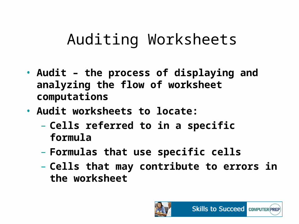
Auditing Worksheets

• Audit – the process of displaying and analyzing the flow of worksheet computations

• Audit worksheets to locate:– Cells referred to in a specific formula– Formulas that use specific cells– Cells that may contribute to errors in the

worksheet

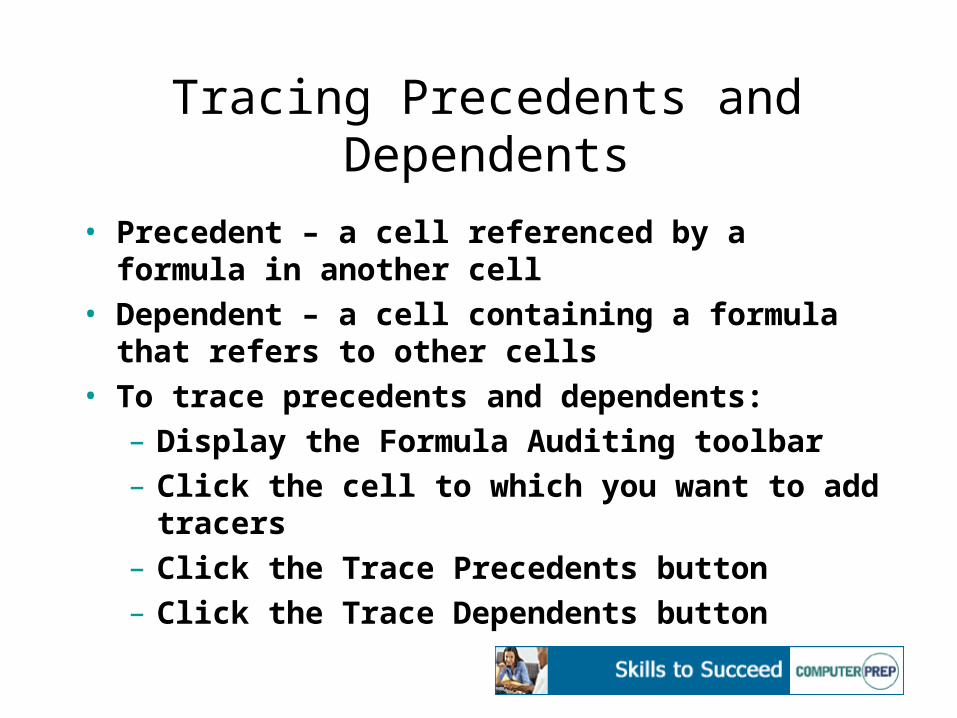
Tracing Precedents and Dependents

• Precedent – a cell referenced by a formula in another cell

• Dependent – a cell containing a formula that refers to other cells

• To trace precedents and dependents:– Display the Formula Auditing toolbar– Click the cell to which you want to add tracers– Click the Trace Precedents button – Click the Trace Dependents button

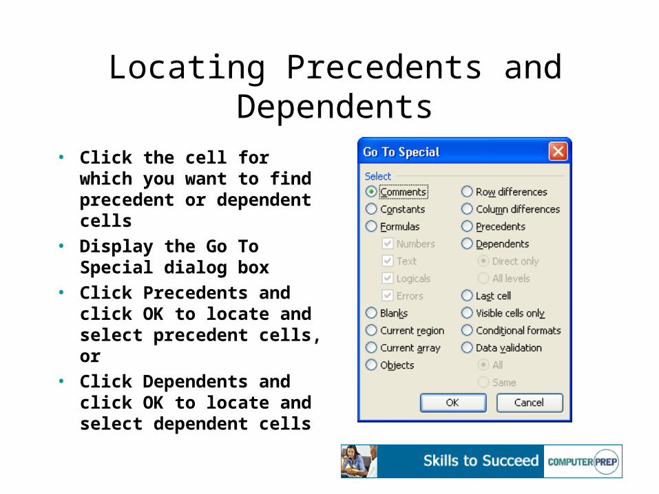
Locating Precedents and Dependents

• Click the cell for which you want to find precedent or dependent cells

• Display the Go To Special dialog box

• Click Precedents and click OK to locate and select precedent cells, or

• Click Dependents and click OK to locate and select dependent cells

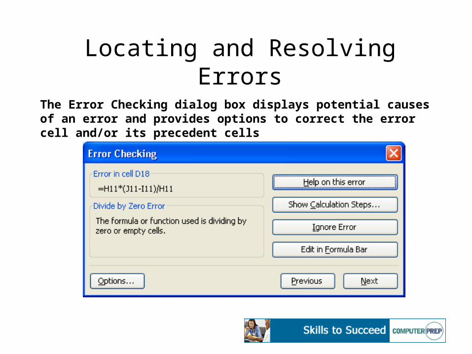
Locating and Resolving Errors

The Error Checking dialog box displays potential causes of an error and provides options to correct the error cell and/or its precedent cells

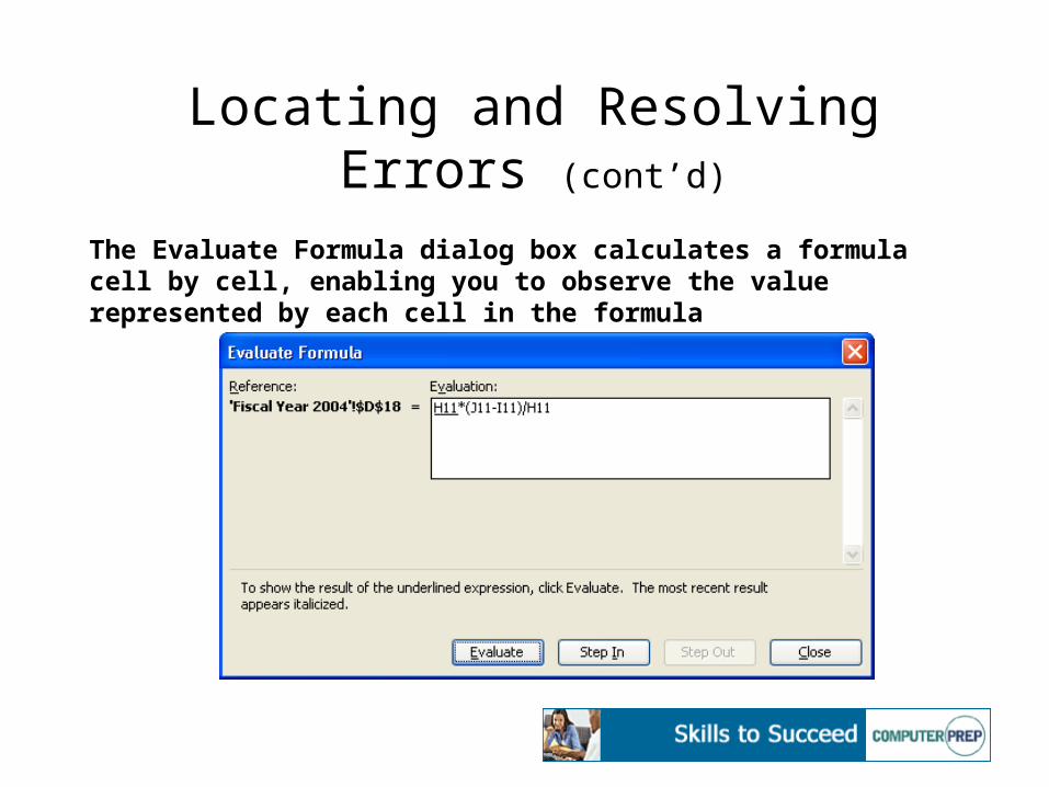
Locating and Resolving Errors (cont’d)

The Evaluate Formula dialog box calculates a formula cell by cell, enabling you to observe the value represented by each cell in the formula

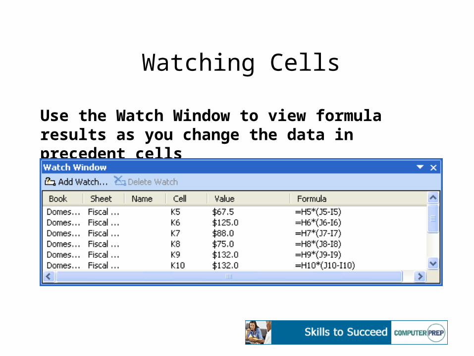
Watching Cells

Use the Watch Window to view formula results as you change the data in precedent cells

Circling Invalid Data

Use the circle invalid data feature to visually highlight any cell data that does not meet data validation criteria you specify for the database field

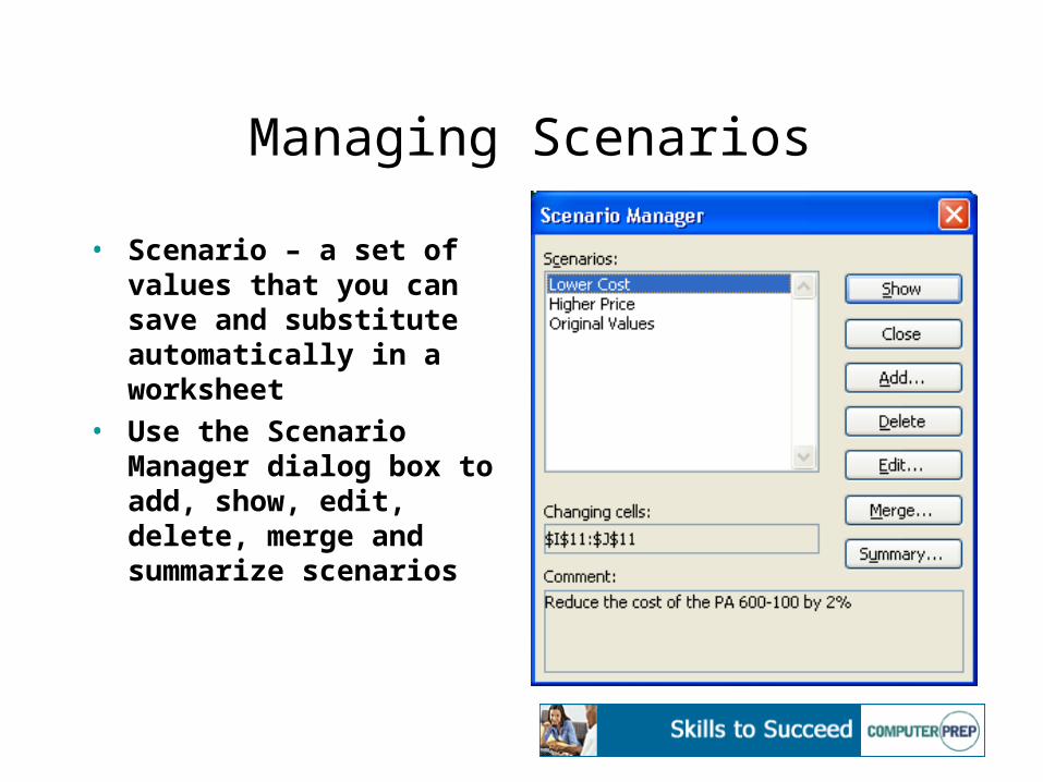
Managing Scenarios

• Scenario – a set of values that you can save and substitute automatically in a worksheet

• Use the Scenario Manager dialog box to add, show, edit, delete, merge and summarize scenarios

Adding Scenarios• To add a scenario from the

Scenario Manager:

– Display the Add Scenario dialog box

– Specify a scenario name

– Specify the adjustable cells

– Specify a comment (optional)

– Display the Scenario Values dialog box

– Specify the different values you want to display in the adjustable cells

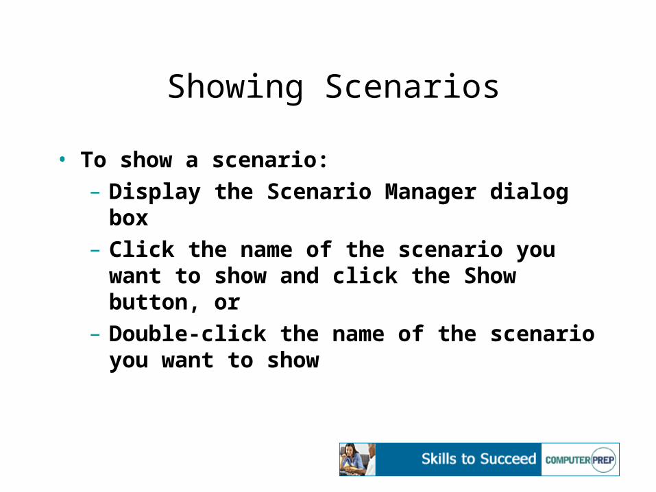
Showing Scenarios

• To show a scenario:– Display the Scenario Manager dialog box– Click the name of the scenario you want to

show and click the Show button, or– Double-click the name of the scenario you want

to show

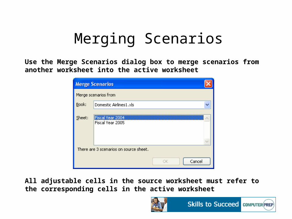
Merging ScenariosUse the Merge Scenarios dialog box to merge scenarios from another worksheet into the active worksheet

All adjustable cells in the source worksheet must refer to the corresponding cells in the active worksheet

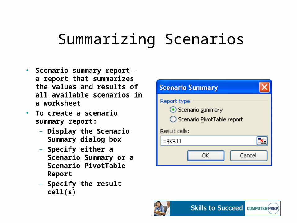
Summarizing Scenarios

• Scenario summary report – a report that summarizes the values and results of all available scenarios in a worksheet

• To create a scenario summary report:

– Display the Scenario Summary dialog box

– Specify either a Scenario Summary or a Scenario PivotTable Report

– Specify the result cell(s)

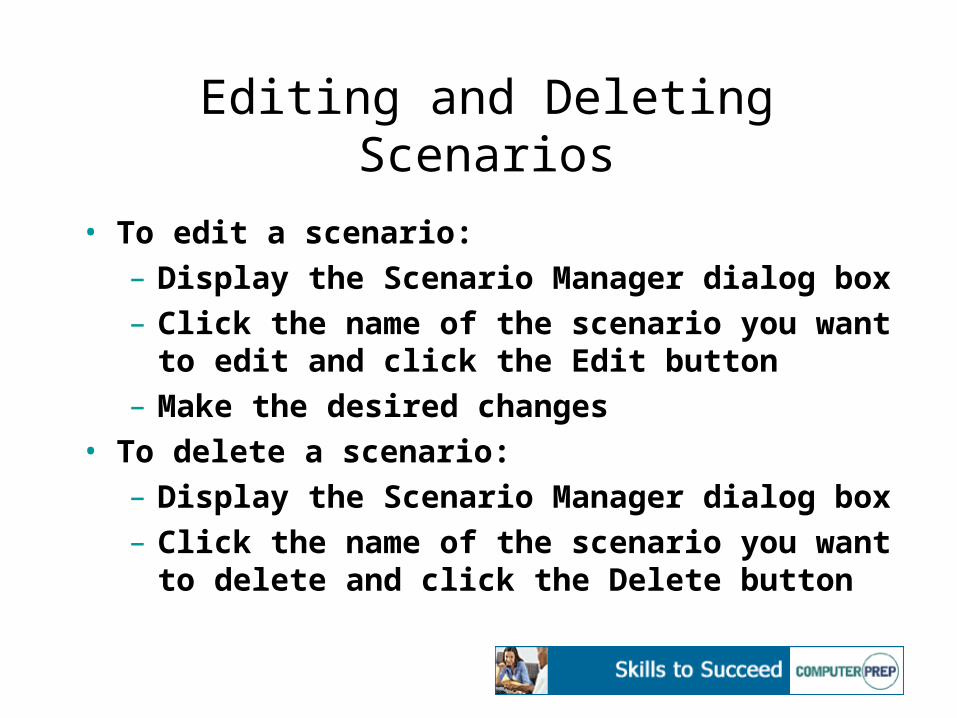
Editing and Deleting Scenarios

• To edit a scenario:– Display the Scenario Manager dialog box– Click the name of the scenario you want to edit

and click the Edit button– Make the desired changes

• To delete a scenario:– Display the Scenario Manager dialog box– Click the name of the scenario you want to

delete and click the Delete button

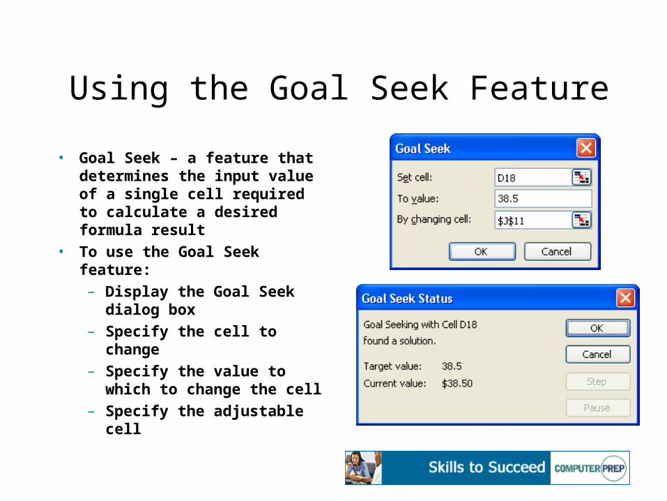
Using the Goal Seek Feature

• Goal Seek – a feature that determines the input value of a single cell required to calculate a desired formula result

• To use the Goal Seek feature:

– Display the Goal Seek dialog box

– Specify the cell to change

– Specify the value to which to change the cell

– Specify the adjustable cell

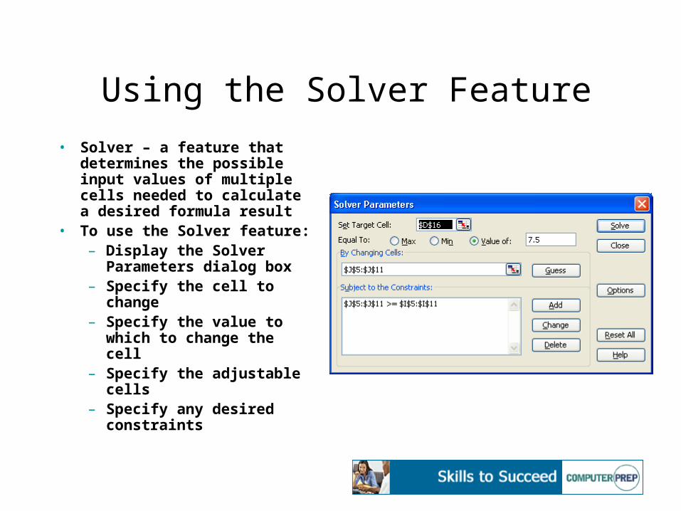
Using the Solver Feature

• Solver – a feature that determines the possible input values of multiple cells needed to calculate a desired formula result

• To use the Solver feature:– Display the Solver

Parameters dialog box– Specify the cell to change– Specify the value to

which to change the cell– Specify the adjustable

cells– Specify any desired

constraints

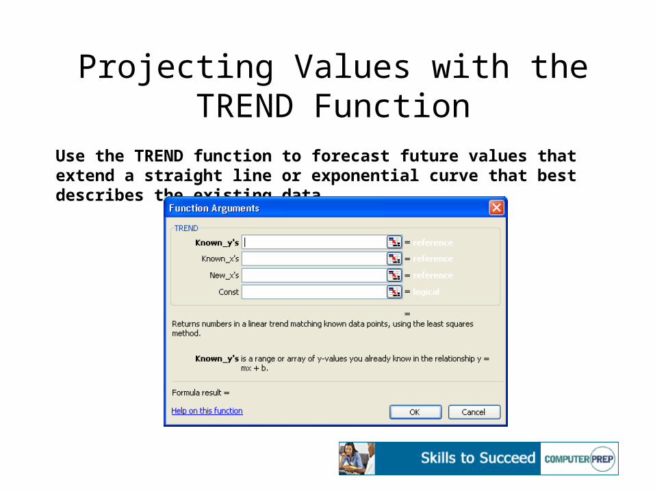
Projecting Values with the TREND Function

Use the TREND function to forecast future values that extend a straight line or exponential curve that best describes the existing data

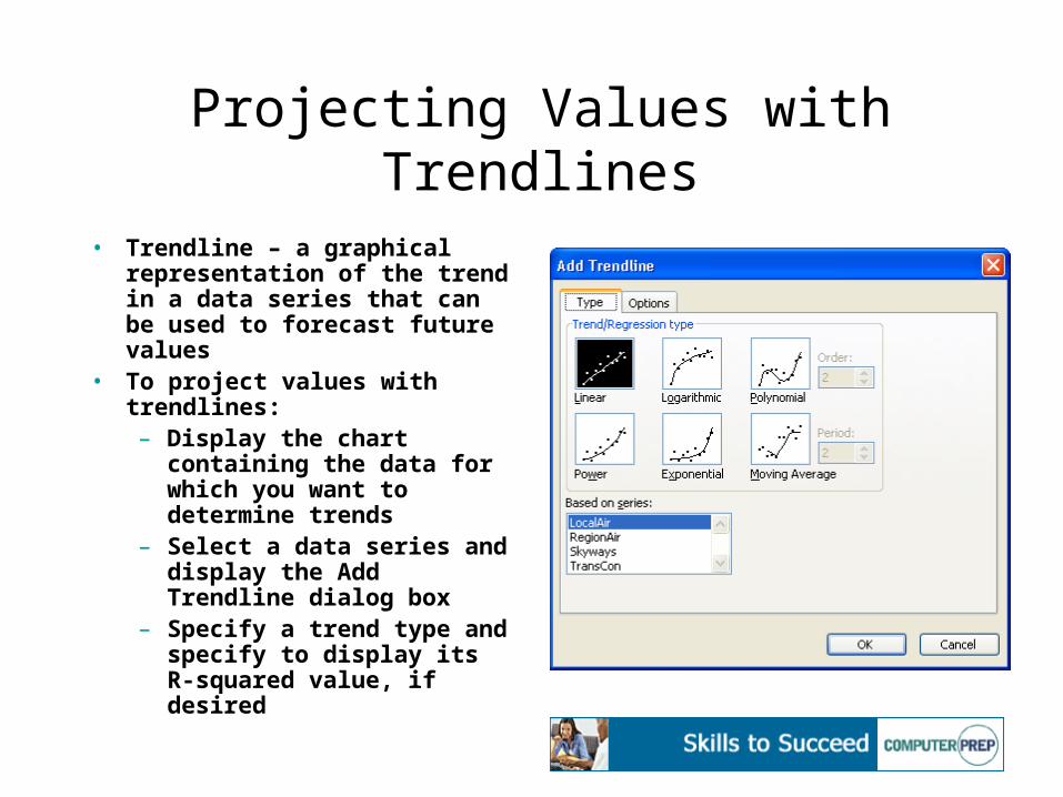
Projecting Values with Trendlines

• Trendline – a graphical representation of the trend in a data series that can be used to forecast future values

• To project values with trendlines:– Display the chart

containing the data for which you want to determine trends

– Select a data series and display the Add Trendline dialog box

– Specify a trend type and specify to display its R-squared value, if desired

© 2001 ComputerPREP, Inc. All rights reserved.

Lesson 3:Using Templates, Range Names and

Advanced Formatting Features

Objectives

• Create and edit templates• Name ranges• Use range names in formulas• Create custom number formats• Use conditional formatting• Format graphics• Format diagrams• Format charts

Creating Templates

• Template – a workbook used to create other workbooks that will contain the same components, formatting and page layout

• When you create a template:– Include the text, graphics, formatting, and so on

that will display in all workbooks you create with the template

– Do not include data that will vary from workbook to workbook

Creating Templates (cont’d)

• To create a template:– Open (or create) the workbook from which you

will create the template– Save the workbook as a template (*.xlt)

• To create a new workbook based on a template:– Display the Templates dialog box – Double-click the name of the template on which

you want to base the new workbook– Enter data in the data entry cells and save the

workbook with a new name

Editing Templates

• Edit templates just as you would edit any workbook you create in Excel

• To edit a template:– Open a new workbook based on the template– Edit the workbook– Save the edited workbook over the original

template

Naming Ranges

• You can name ranges using the:

– Define Name dialog box

– Create Names dialog box

– Name Box

• Naming conventions:

– The first character must be a letter or underscore; remaining characters can be letters, numbers, periods or underscores

– Cell references and spaces cannot be used

– Names can contain up to 255 characters

– Names are not case-sensitive

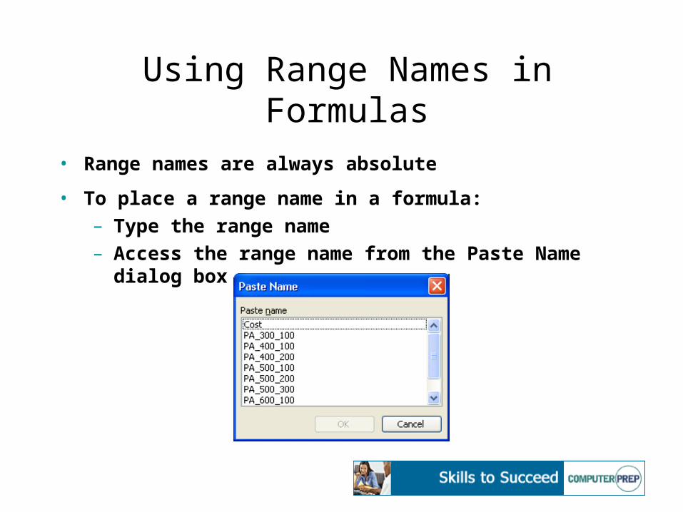
Using Range Names in Formulas

• Range names are always absolute

• To place a range name in a formula:– Type the range name– Access the range name from the Paste Name dialog box

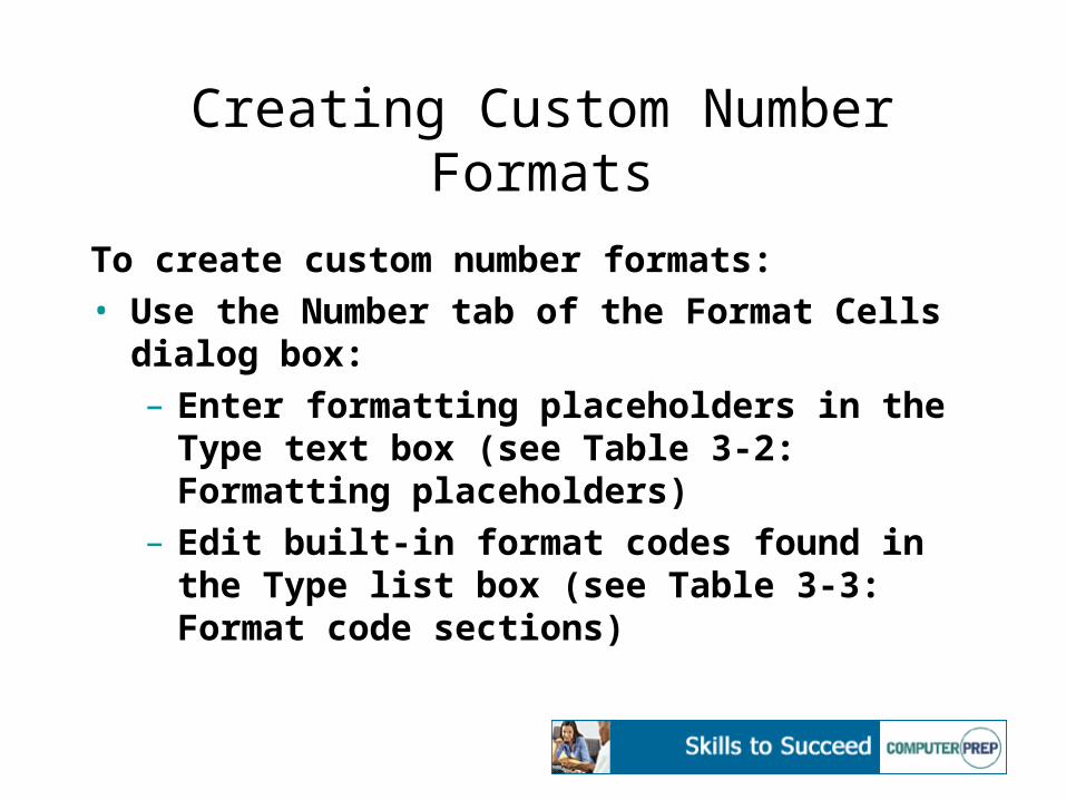
Creating Custom Number Formats

To create custom number formats:• Use the Number tab of the Format Cells dialog

box:– Enter formatting placeholders in the Type text

box (see Table 3-2: Formatting placeholders)– Edit built-in format codes found in the Type list

box (see Table 3-3: Format code sections)

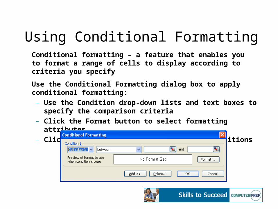
Using Conditional FormattingConditional formatting – a feature that enables you to format a range of cells to display according to criteria you specify

Use the Conditional Formatting dialog box to apply conditional formatting:

– Use the Condition drop-down lists and text boxes to specify the comparison criteria

– Click the Format button to select formatting attributes

– Click the Add button to add up to three conditions

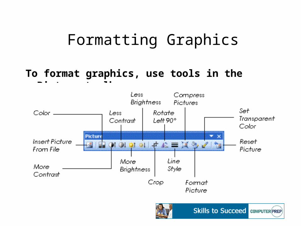
Formatting Graphics

To format graphics, use tools in the Picture toolbar:

Formatting Diagrams

To format diagrams:– Use the Format AutoShape dialog box to

specify formatting options for a particular diagram component

– Use the Format Diagram dialog box to specify formatting options for the diagram as a whole

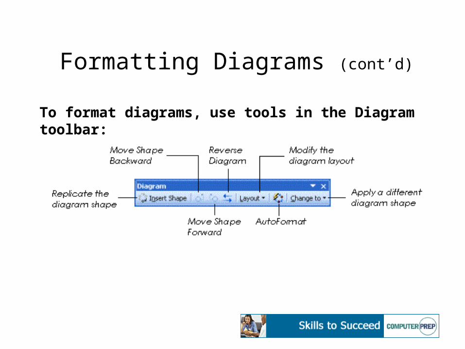
Formatting Diagrams (cont’d)

To format diagrams, use tools in the Diagram toolbar:

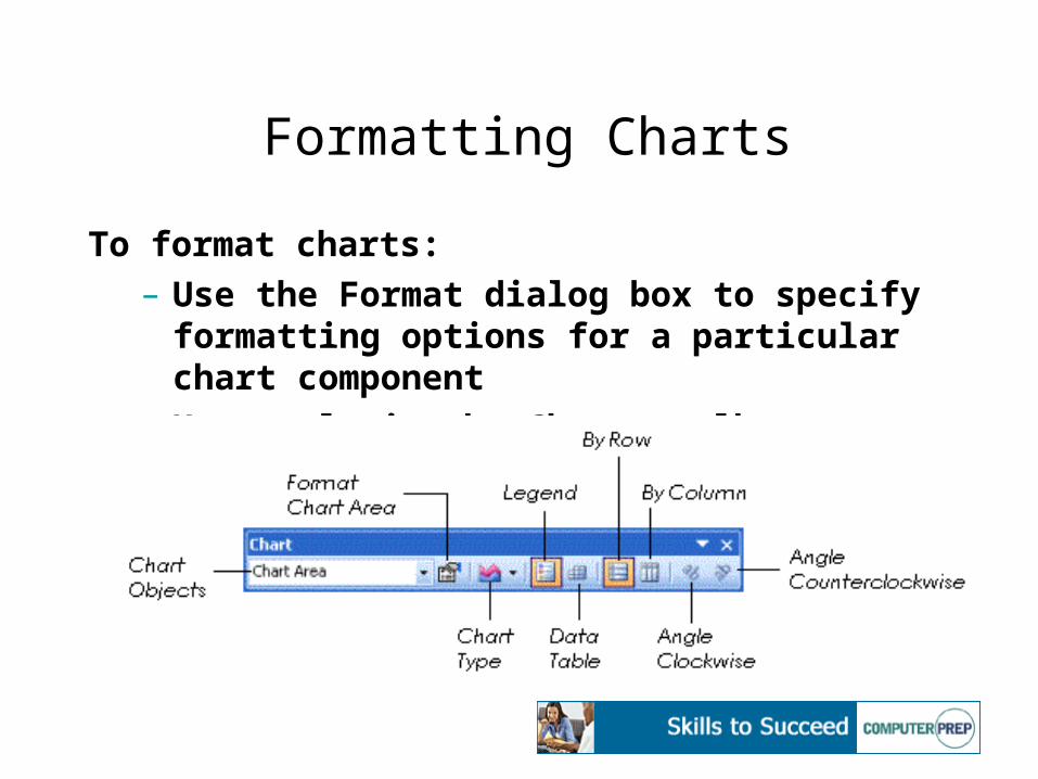
Formatting Charts

To format charts:– Use the Format dialog box to specify formatting

options for a particular chart component– Use tools in the Chart toolbar:

© 2001 ComputerPREP, Inc. All rights reserved.

Lesson 4:Using Protection and Collaboration

Features

Objectives

• Manage workbook properties• Protect data• Manage workbook security• Create shared workbooks• Track changes• Accept and reject changes• Merge workbooks

Managing Workbook Properties

• View and set workbook properties using the five tabs in the Properties dialog box:– General – displays the file name, type, location, size,

creation date, last modification date, and so on– Summary – enables you to add specific information about

the workbook– Statistics – displays the creation date and the last time

the workbook was modified, accessed, printed and saved– Contents – displays the names of worksheets, charts,

reports and macro sheets– Custom – enables you to create your own custom

properties

Protecting Workbooks

• Workbook protection – safeguards the structure and onscreen appearance of a workbook from certain types of modification– Structure protection prevents:

• Viewing hidden worksheets• Moving, deleting, hiding, or renaming worksheets• Inserting new worksheets• Moving or copying worksheets to another workbook

– Windows protection prevents:• Changing the size and position of the window• Moving, resizing or closing the window

Protecting Worksheets

• Worksheet protection – prevents you and others from entering or modifying data in a worksheet

• You must protect worksheets individually to prevent unauthorized modification (this enables protection of certain worksheets while allowing modification of other, unprotected worksheets)

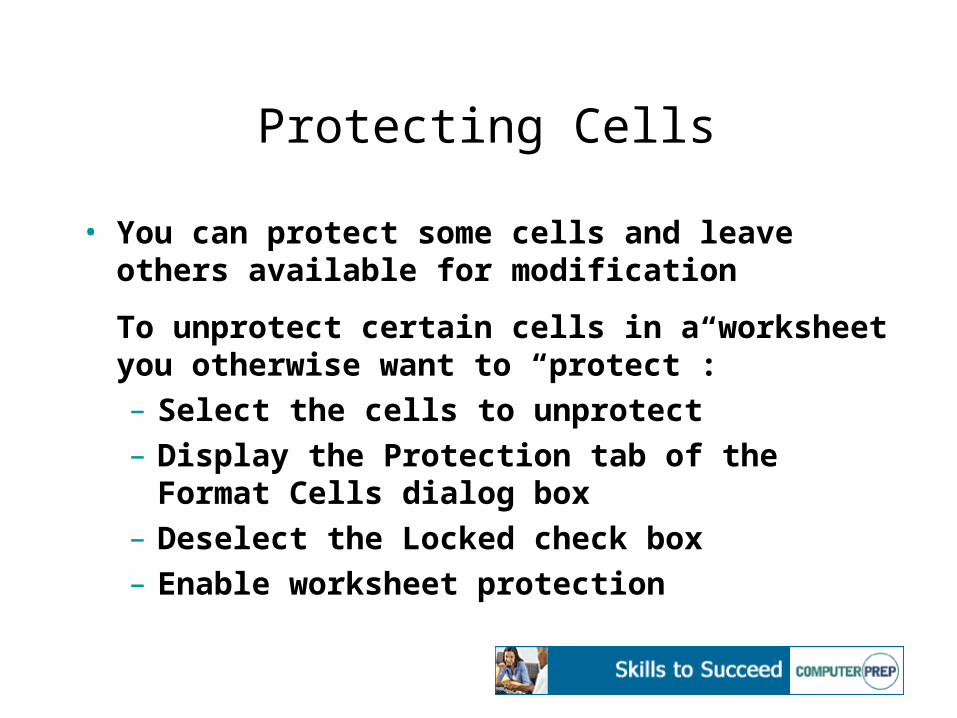
Protecting Cells

• You can protect some cells and leave others available for modification

To unprotect certain cells in a worksheet you otherwise want to “protect”:– Select the cells to unprotect– Display the Protection tab of the Format Cells

dialog box– Deselect the Locked check box– Enable worksheet protection

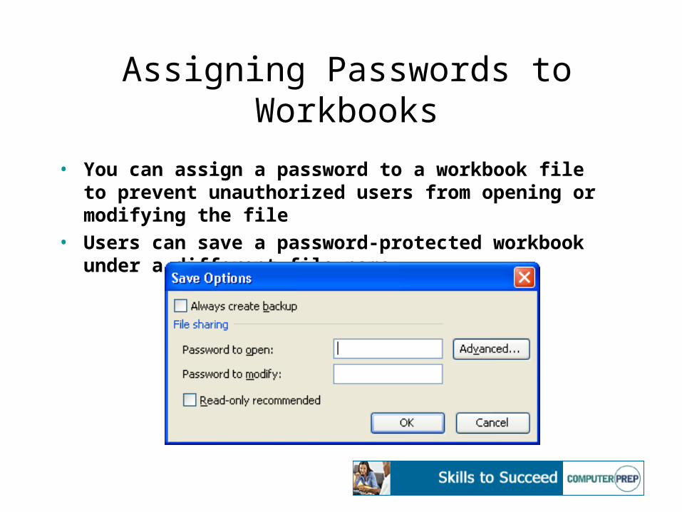
Assigning Passwords to Workbooks

• You can assign a password to a workbook file to prevent unauthorized users from opening or modifying the file

• Users can save a password-protected workbook under a different file name

Setting Macro Security Levels

• Set macro security levels to detect macros, which may contain viruses

• You can specify four levels of security:– Very High – all macros will be disabled.– High – all macros from trusted sources will run.

You will be prompted about unknown macros. Unsigned macros will be disabled.

– Medium – all macros from trusted sources will run. You will be prompted about unknown macros.

– Low – all macros will run.

Using Digital Signatures

• Use a digital signature to authenticate a workbook• Use a digital certificate to digitally sign a file

– Digital certificate – an attachment to a file that vouches for its authenticity, provides secure encryption or supplies a verifiable signature

Creating Shared Workbooks

• Shared workbook – a workbook that has been set up to allow multiple users on a network to view and edit the workbook simultaneously

• Once a workbook is shared, Excel keeps track of all changes by you and other users by maintaining a change history– Change history – a log of all changes made to a

shared workbook during a specified time period

Tracking Changes

• When you share a workbook, Excel automatically keeps track of changes made by you and other users

• When you activate tracked changes, changed cells are surrounded by blue boxes with a triangle in the upper-left corner

• The column and row indicators for the changed cells display in red

• When you position the mouse pointer over a changed cell, a comment displays describing the change

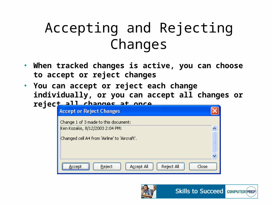
Accepting and Rejecting Changes

• When tracked changes is active, you can choose to accept or reject changes

• You can accept or reject each change individually, or you can accept all changes or reject all changes at once

Merging Workbooks

• You can merge workbooks to join all changes together• Before merging, workbooks must meet the following

requirements:– Workbooks must be copies of the same shared workbook– Each copy must have a different file name – The workbooks must either not have passwords or all

have the same password– Tracked changes in all workbooks must be in effect

continuously from the time the copies were made– Change history must be active and go back at least as far

as the date when the copies were made– The shared workbooks must reside in the same folder

© 2001 ComputerPREP, Inc. All rights reserved.

Lesson 5:Using Consolidation, Web,

Integration and XML Features

Objectives

• Consolidate data from multiple worksheets• Save workbooks as Web pages• Publish workbooks to the Web• Import data into Excel• Export data from Excel• Structure workbooks using XML

Consolidating Data from Multiple Worksheets

• Consolidate – to combine values from multiple ranges of data

• Methods to consolidate data:– Create 3-dimensional formulas– Consolidate data by position– Consolidate data by category

• To consolidate data by position or by category, source ranges:– Must be laid out in list format– Must display on separate worksheets

Consolidating Data from Multiple Worksheets (cont’d)

• 3-dimensional formulas contain references to cells in other worksheets

• Consolidate by position when all ranges containing the source data are identical in structure and layout

• Consolidate by category if the source data ranges have matching column and/or row labels but are not necessarily laid out similarly

Saving Workbooks as Web Pages

• Saving workbooks as Web pages enables you to view them in your browser

• You can save an entire workbook or individual worksheets

• All formatting attributes are retained• You can preview what the workbook will look like

in your browser using Web Page Preview

Publishing Workbooks to the Web

• You can publish individual worksheets or an entire workbook to the Web

• Your workbook/worksheet becomes interactive and can be manipulated in the Web browser

• You must have Microsoft Internet Explorer 5.01 or later to enable interactivity

Importing Data from a Data Source

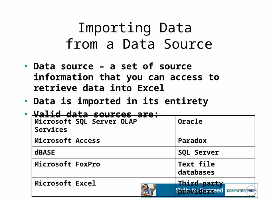
• Data source – a set of source information that you can access to retrieve data into Excel

• Data is imported in its entirety• Valid data sources are:

Microsoft SQL Server OLAP Services Oracle

Microsoft Access Paradox

dBASE SQL Server

Microsoft FoxPro Text file databases

Microsoft Excel Third-party providers

Importing Data using Microsoft Query

• Use the Query Wizard to import data from a data source when you want to specify specific items of data to import, such as:– Which fields to import– Which records to import– The sort order of the imported data

Importing Data from the Web

• Click the desired table selection buttons to select or deselect the tables of data in the Web page to import– Press and hold SHIFT while clicking to select or

deselect multiple tables at the same time• When you specify to import the Web data into

Excel, all selected tables will be imported

Exporting Data from Excel

• Excel data must be in list format for it to be used by other applications

• To export Excel data, you actually import the data from within the application in which you want to use the data

Introducing XML

• Excel’s XML capabilities enable you to retrieve XML data into Excel– Extensible Markup Language (XML) – a format

for delivering rich, structured data from an application in a standard, consistent manner

• To retrieve XML data, attach an XML schema to a workbook– Schema – A file containing XML tags that

defines the structure of a database

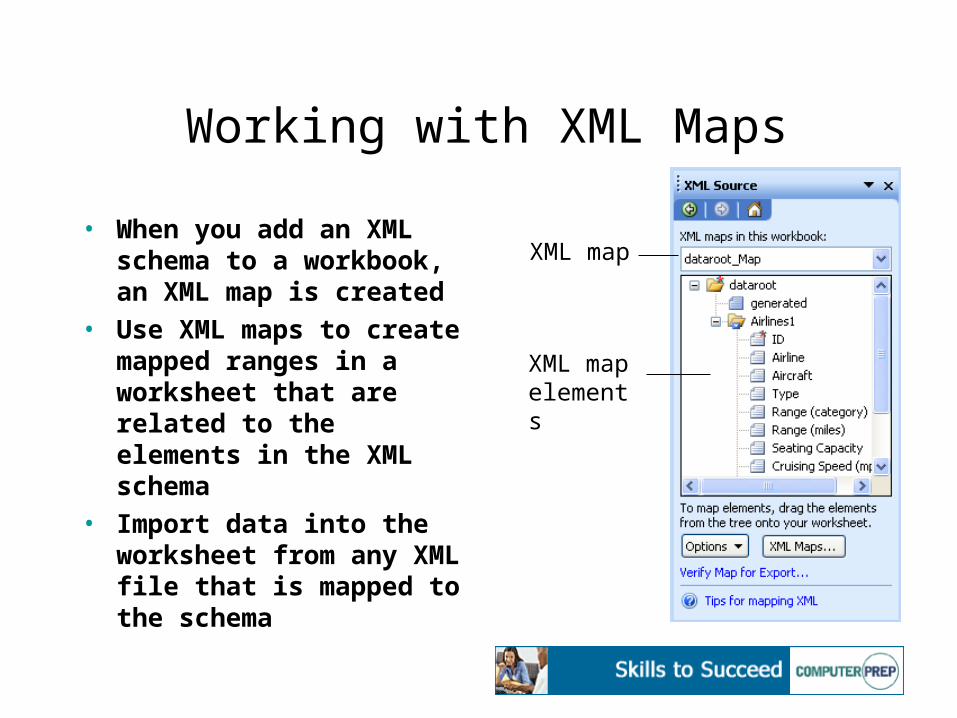
Working with XML Maps

• When you add an XML schema to a workbook, an XML map is created

• Use XML maps to create mapped ranges in a worksheet that are related to the elements in the XML schema

• Import data into the worksheet from any XML file that is mapped to the schema

XML map

XML mapelements

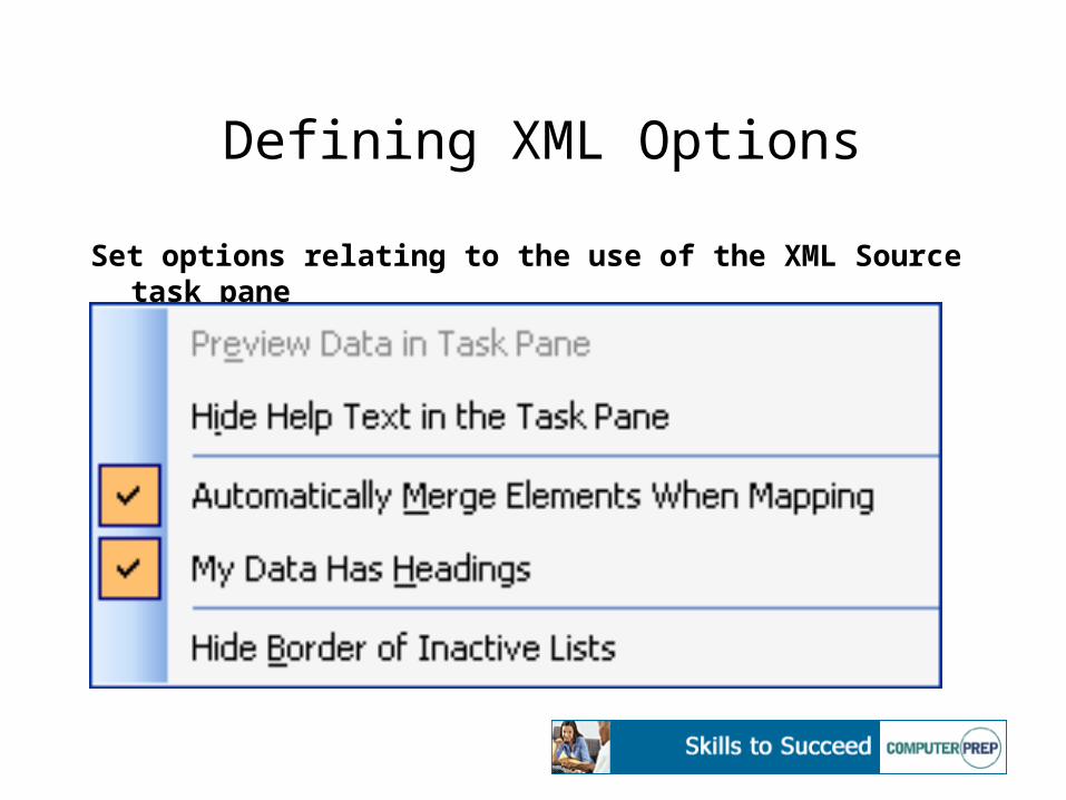
Defining XML Options

Set options relating to the use of the XML Source task pane

Modifying XML Workbook Elements

• Use the XML map elements to create mapped ranges in your workbook

• You can manipulate the mapped ranges, or lists, just as you do any data you create in Excel

• Each mapped range acts as a single unit when moved or copied

© 2001 ComputerPREP, Inc. All rights reserved.

Lesson 6:Customizing Excel and Using Macros

Objectives

• Modify default settings• Customize toolbars• Customize menus• Create and edit macros

Modifying Default Settings

• Modify default settings to change the default appearance and operation of Excel

• To modify default settings:– Display the Options dialog box– Click the tab containing the settings you want

to change– Change the desired options

• Once settings are modified, they remain that way until you change them again

Creating Custom Toolbars

• Create a custom toolbar to contain command buttons you use frequently that are in several different toolbars

• To create a custom toolbar:– Display the Toolbars tab of the Customize

dialog box and click the New button– Specify a name for the custom toolbar– Display the Commands tab and drag the

command buttons you want to the custom toolbar

Manipulating Toolbar Buttons

• You can add, delete and rearrange toolbar buttons on any toolbar by dragging them while the Customize dialog box is open

• If the Customize dialog box is closed:– To move a button: press and hold ALT and drag

the button– To copy a button: press and hold CTRL+ALT

and drag the button– To delete a button: press and hold ALT and

drag the button into the worksheet area

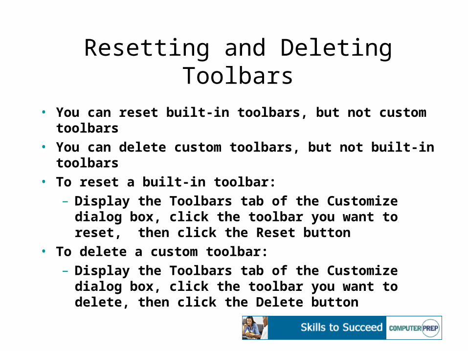
Resetting and Deleting Toolbars

• You can reset built-in toolbars, but not custom toolbars

• You can delete custom toolbars, but not built-in toolbars

• To reset a built-in toolbar:

– Display the Toolbars tab of the Customize dialog box, click the toolbar you want to reset, then click the Reset button

• To delete a custom toolbar:

– Display the Toolbars tab of the Customize dialog box, click the toolbar you want to delete, then click the Delete button

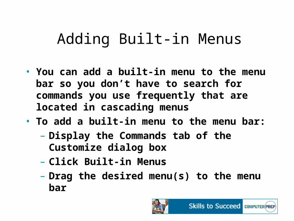
Adding Built-in Menus

• You can add a built-in menu to the menu bar so you don’t have to search for commands you use frequently that are located in cascading menus

• To add a built-in menu to the menu bar:– Display the Commands tab of the Customize

dialog box– Click Built-in Menus– Drag the desired menu(s) to the menu bar

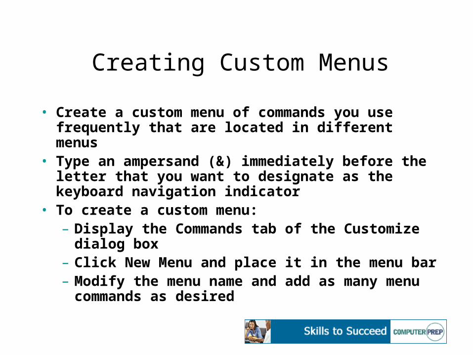
Creating Custom Menus

• Create a custom menu of commands you use frequently that are located in different menus

• Type an ampersand (&) immediately before the letter that you want to designate as the keyboard navigation indicator

• To create a custom menu:– Display the Commands tab of the Customize

dialog box– Click New Menu and place it in the menu bar– Modify the menu name and add as many menu

commands as desired

Recording Macros

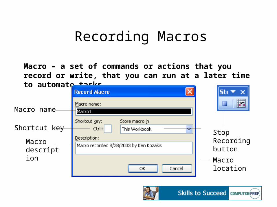
Macro – a set of commands or actions that you record or write, that you can run at a later time to automate tasks

Stop Recording button

Macro name

Shortcut key

Macro location

Macro description

Running Macros

• When you run a macro, the recorded commands execute automatically

• To run a macro:– Press the shortcut key you assigned when you

recorded the macro, or– Display the Macro dialog box, click the macro

name, then click the Run button

Editing Macro Code

• Macro commands are recorded in Visual Basic• To edit macro code:

– Display the Macro dialog box– Click the desired macro and click the Edit

button to display the macro in the Visual Basic Editor

– Make the desired changes and close the Visual Basic Editor