© 2011 jason a. webber. all rights reserved
TRANSCRIPT

© 2011 Jason A. Webber. All rights reserved.

COLLIMATION OF DEUTERIUM / 3-HELIUM FUSION PRODUCTS FOR ADVANCED SPACECRAFT PROPULSION AND POWER
BY
JASON A. WEBBER
THESIS
Submitted in partial fulfillment of the requirements for the degree in Master of Science of Nuclear Engineering
in the Graduate College of the University of Illinois Urbana-Champaign, 2011
Urbana, Illinois
Master’s Committee:
Professor Emeritus George H. Miley, Chair Professor Emeritus Rodney L. Burton Assistant Professor Brian E. Jurczyk
ii
Abstract
COLLIMATION OF d-He3 FUSION PRODUCTS FOR ADVANCED SPACECRAFT PROPULSION AND POWER
Jason A. Webber
Department of Nuclear, Plasma, and Radiological Engineering University of Illinois at Urbana-Champaign, 2011
Dr. George H. Miley, Advisor
Current space exploration has transpired through the use of chemical rockets, and they
have served us well, but they have their limitations. Exploration of the outer solar system,
Jupiter and beyond will most likely require a new generation of propulsion system. One
potential technology class to provide spacecraft propulsion and power systems involve
thermonuclear fusion plasma systems. In this class it is well accepted that d-He3 fusion is
the most promising of the fuel candidates for spacecraft applications1 as the 14.7 MeV
protons carry up to 80% of the total fusion power while α‘s have energies less than 4
MeV. The other minor fusion products from secondary d-d reactions consisting of 3He, n,
p, and 3H also have energies less than 4 MeV. Furthermore there are two main fusion
subsets namely, Magnetic Confinement Fusion devices and Inertial Electrostatic
Confinement (or IEC) Fusion devices. Magnetic Confinement Fusion devices are
characterized by complex geometries and prohibitive structural mass compromising
spacecraft use at this stage of exploration. While generating energy from a lightweight
and reliable fusion source is important, another critical issue is harnessing this energy
into usable power and/or propulsion. IEC fusion is a method of fusion plasma
confinement that uses a series of biased electrodes that accelerate a uniform spherical
beam of ions into a hollow cathode typically comprised of a gridded structure with high
transparency. The inertia of the imploding ion beam compresses the ions at the center of
the cathode increasing the density to the point where fusion occurs. Since the velocity
distributions of fusion particles in an IEC are essentially isotropic and carry no net
momentum, a means of redirecting the velocity of the particles is necessary to efficiently
extract energy and provide power or create thrust. There are classes of advanced fuel
fusion reactions where direct-energy conversion based on electrostatically-biased
collector plates is impossible due to potential limits, material structure limitations, and

iii
IEC geometry. Thermal conversion systems are also inefficient for this application. A
method of converting the isotropic IEC into a collimated flow of fusion products solves
these issues and allows direct energy conversion. An efficient traveling wave direct
energy converter has been proposed and studied by Momota2, Shu3 and further studied by
evaluated with numerical simulations by Ishikawa4 and others.
One of the conventional methods of collimating charged particles is to surround the
particle source with an applied magnetic channel. Charged particles are trapped and move
along the lines of flux. By introducing expanding lines of force gradually along the
magnetic channel, the velocity component perpendicular to the lines of force is
transferred to the parallel one. However, efficient operation of the IEC requires a null
magnetic field at the core of the device. In order to achieve this, Momota5 and Miley have
proposed a pair of magnetic coils anti-parallel to the magnetic channel creating a null
hexapole magnetic field region necessary for the IEC fusion core.
Numerically, collimation of 300 eV electrons without a stabilization coil was
demonstrated to approach 95% at a profile corresponding to Vsolenoid = 20.0V, Ifloating =
2.78A, Isolenoid = 4.05A while collimation of electrons with stabilization coil present was
demonstrated to reach 69% at a profile corresponding to Vsolenoid = 7.0V, Istab = 1.1A,
Ifloating = 1.1A, Isolenoid = 1.45A.
Experimentally, collimation of electrons with stabilization coil present was demonstrated
experimentally to be 35% at 100 eV and reach a peak of 39.6% at 50eV with a profile
corresponding to Vsolenoid = 7.0V, Istab = 1.1A, Ifloating = 1.1A, Isolenoid = 1.45A and
collimation of 300 eV electrons without a stabilization coil was demonstrated to approach
49% at a profile corresponding to Vsolenoid = 20.0V, Ifloating = 2.78A, Isolenoid = 4.05A
6.4% of the 300eV electrons’ initial velocity is directed to the collector plates. The
remaining electrons are trapped by the collimator’s magnetic field. These particles
oscillate around the null field region several hundred times and eventually escape to the
collector plates.
iv
At a solenoid voltage profile of 7 Volts, 100 eV electrons are collimated with wall and
perpendicular component losses of 31%. Increasing the electron energy beyond 100 eV
increases the wall losses by 25% at 300 eV. Ultimately it was determined that a field
strength deriving from 9.5 MAT/m would be required to collimate 14.7 MeV fusion
protons from d-3He fueled IEC fusion core.
The concept of the proton collimator has been proven to be effective to transform an
isotropic source into a collimated flow of particles ripe for direct energy conversion.

v
In memory of James R. Webber & Dr. Andrei Lipson

vi
Acknowledgements
There are so many people to whom I owe a debt of gratitude, and I apologize for anyone
that I forgot to mention.
The road taken to get to this point can certainly be described as the scenic route. Many
times I would stop off the trail to investigate the wonders of this universe, but eventually
returned to the road, sometimes kicking and scream, continuing onward to the goal.
I would first like to thank Prof. George H. Miley, my advisor, whose patience,
understanding, and encouragement made all of this possible. Sometimes when I had lost
my way he was always there to help me get back on the trail. No other advisor could have
given me quite the freedom to make my own mistakes and still find the discoveries
sometimes accidental that made the journey so fulfilling. You have been much kinder
than I ever deserved. Thank you.
Dr. Rodney Burton and Dr. Brian Jurczyk I would like to deeply thank for both acting in
the unusual role of dual readers for this manuscript. I have always admired both of you
greatly.
I would like to thank Dr. H. Momota for his great patience and insight on the theoretical
work that became the basis of this undertaking, Dr. Martin Nieto-Perez for his M.S.
efforts that greatly contributed to this work, and Dr. Rodney Burton for his insight, time,
and ideas that kept me thinking about the aerospace end game on this project.
Dr. Robert Stubbers was instrumental in the formative stages of this project. It was
comforting to always know I had an open door and open minds to bounce ideas off of.
Everyone should be so lucky to have that asset.

vii
Hyung-Jin Kim and Linchun Wu were a big part of this work as well, constructing the
magnetic coils, extensive personal communications, and many other aspects of project
integration.
Thanks to the National Aeronautics and Space Administration for the grant that funded
the design, construction, and testing of the proton collimator simulator.
There are a number of people whose encouragement and example helped me to keep at it
when I began to lose sight of the goal: Ben Masters, Ryan Ruzic, Brandon Ruzic, Vikram
Chaudhery, Patrick Lynch, Zenobia Ravji, Jaclyn O’Day, Kelley Young, Diane Webber,
Becky Meline, Rhonda Kirts, Professor Nicholas Petruzzi, Professor R. A. Axford, and
Dean Larry DeBrock. You are not forgotten.
I also would like thank Major Edward A. Dames (Ret.) who gave me an almost
unimaginable tool capable of solving any problem in time and space.
Finally, a special thank you to Dean Paul Brown, who gave me the chance...
viii
Table of Contents List of Figures ..................................................................................................................... x List of Tables .................................................................................................................... xv List of Abbreviations ....................................................................................................... xvi Chapter 1 Introduction & Background ............................................................................... 1
1.1 IEC Reactor & Fusion Products ................................................................................ 2 1.2 Application to Spacecraft Power & Propulsion ........................................................ 7 1.3 Application of Fusion System to Prospective Spacecraft Designs ......................... 12 1.4 Research Objectives & Scientific Relevance .......................................................... 13
Chapter 2 Proton Collimation ........................................................................................... 15 2.1 Theoretical Description of the Proton Collimator .................................................. 15 2.2 Scaling from a Proton Device to an Electron Simulation ....................................... 22
Chapter 3 Experiment Device Configuration ................................................................... 26 3.1 Vacuum Chamber ................................................................................................... 26 3.2 Solenoidal Coils ...................................................................................................... 30 3.3 Floating Coils .......................................................................................................... 31 3.4 Collector Plates ....................................................................................................... 37
3.4.1 Axial Electron Plates ........................................................................................ 37 3.4.2 Radial Electron Plates ...................................................................................... 38
3.5 Electron Sources ..................................................................................................... 40 3.5.1 Spherical .......................................................................................................... 40 3.5.2 Electron Gun .................................................................................................... 45
Chapter 4 Overview of Experiments................................................................................. 53 4.1 Extractor Setup and Testing .................................................................................... 53 4.2 Null Magnetic Field Settings .................................................................................. 55
Chapter 5 Results .............................................................................................................. 61 5.1 Collimation ............................................................................................................. 61 5.2 Scattering – Reverse Mode Configuration .............................................................. 68 5.3 Collimated Particle Energy ..................................................................................... 80
Chapter 6 Interpretation .................................................................................................... 83 6.1 Collimation Efficiency ............................................................................................ 83
Chapter 7 Particle Simulation ........................................................................................... 88 7.1 Numerical Considerations ....................................................................................... 89 7.2 Magnetic Coil Modeling ......................................................................................... 90 7.3 Isotropic Plasma Source .......................................................................................... 91 7.4 Cases Simulated ...................................................................................................... 93

ix
7.5 Evidence of Collimation Results ............................................................................ 94 7.6 Stabilization Coil LOAD Scenario Simulation Results .......................................... 95 7.7 Stabilization Coil Scenario Simulation Results ...................................................... 96 7.8 Sans-Stabilization Coil Scenario Simulation Results ........................................... 104
Chapter 8 Conclusions & Future Work .......................................................................... 107 Appendix A: Biot-Savart Base Input File ...................................................................... 112 Appendix B: OOPIC Load Input File Subsection........................................................... 113 Appendix C: OOPIC Base Input File.............................................................................. 114 Appendix D: Electron Gun Additions to OOPIC Input File ........................................... 138 Appendix E: Double Collimator OOPIC Input File ....................................................... 140 References ....................................................................................................................... 178 Authors Biography……………………………………………………………………….………………….…180

x
List of Figures
Figure 1: Inertial Electrostatic Confinement Fusion Device at the Fusion Studies Laboratory. .......................................................................................................................... 3 Figure 2: Fusion cross-sections for d – 3He reactions7. ...................................................... 5 Figure 3: The proposed magnetic coil configuration used to redirect the isotropic fusion products from the IEC core into a collimated flow along the magnetic channel. ............... 8 Figure 4: Details the composite neutral beam injector IEC with collimator coils for a proposed spacecraft propulsion/power system ................................................................... 9 Figure 5: Traveling Wave Direct Energy Converter ......................................................... 10 Figure 6: Composite magnetic expander (ME), magnetic separator (MS), and traveling wave direct energy converter (TWDEC) configuration. ................................................... 11 Figure 7: Proposed spacecraft propulsion and power system utilizing neutral beam injection IEC fusion devices and traveling wave direct energy converters. ..................... 11 Figure 8: Depiction of the Fusion Vehicle Proposed at STAIF 2002. .............................. 12 Figure 9: Depiction of Fusion Ship II from STAIF 2003. ................................................ 13 Figure 10: Helmholtz coil generated magnetic field showing null field region at origin. 17 Figure 11: Illustration of geometric parameters for coil configuration studies ................ 18 Figure 12: Helmholtz Coils Inside of and Anti-Parallel to a Uniform Magnetic Field Generated From a Solenoid .............................................................................................. 19 Figure 13: Accessible region in center produced by a pair of Helmholtz coils (purple) and an anti-parallel stabilization coil (red) is isolated from both the vacuum chamber and the magnetic coils. The region between the outer lines and circles is the proton accessible region. ............................................................................................................................... 21 Figure 14: Magnetic field flux composite for experimental device. ................................. 25 Figure 15: Magnetic vector potential A ............................................................................ 25 Figure 16 CAD drawing of UHV chamber. ...................................................................... 27 Figure 17 Vacuum Chamber Exterior with Solenoidal Coils. .......................................... 28 Figure 18: Chamber dimensions – diameters.................................................................... 29 Figure 19: Chamber dimensions - angles .......................................................................... 29 Figure 20: Section view of solenoid coil, (a) 3-dimensional cut view, (b) cross section of solenoid coil. ..................................................................................................................... 30 Figure 21: Diagram of solenoid coil support rod (left) and the solenoidal coil assembly (right). ............................................................................................................................... 31 Figure 22: The bifilar technique starting point is detailed. The central wire toroid with equal lengths of magnetic wire at both ends to ensure theta component cancellation is shown. ............................................................................................................................... 32 Figure 23: Bi-filar coil construction technique, both magnetic wire coils are looped ...... 33 Figure 24: Photograph of Completed Floating Coils (left) and Stabilization Coil (right). 33 Figure 25: Internal Coil Geometry of Floating Coils (Purple), Stabilization Coil (Pink), & Electron Source at the origin (white) ................................................................................ 34 Figure 26: Internal layout of electron collimator components with the anode and cathode of the electron source, magnetic coils, collector plates and structural supports. .............. 35 Figure 27: Internal Coil Configuration for the Electron Collimator before Insertion of Electron Source with 1st generation collector plate arrangement ..................................... 36 Figure 28: (a) Diagram of axial collector ring relative positions and (b) the actual collector ring assemblies. .................................................................................................. 37

xi
Figure 29: Improved Collector Plate Configuration ......................................................... 38 Figure 30: Filament-Extractor Grid Setup ........................................................................ 40 Figure 31: Interior view of vacuum chamber showing filament-extractor assembly with the coil arrangement .......................................................................................................... 41 Figure 32: (a) Spherical Filament (0.1-mm Tungsten) and Support Structure and (b) the Spherical Filament while in use ........................................................................................ 42 Figure 33: Experiment spherical filament stabilization and extraction grid concept ....... 43 Figure 34: Study of asymmetrical isotropic electron source on collector plate current ... 44 Figure 35: Diagram of Pierce Diode electron gun as described in Building Scientific Apparatus .......................................................................................................................... 46 Figure 36: Electron gun simulation with 120mm anode-cathode distance ....................... 48 Figure 37: Electron gun simulation with 145mm anode-cathode distance ....................... 48 Figure 38: Electron gun simulation with 170mm anode-cathode distance without collimation ........................................................................................................................ 49 Figure 39: 9mA Electron gun simulation with 145mm anode-cathode distance, and 10V collimation profile ............................................................................................................. 49 Figure 40: 9mA Electron gun simulation with 145mm anode-cathode distance, and 20V collimation profile, ............................................................................................................ 50 Figure 41: Pierce Diode electron gun schematic .............................................................. 50 Figure 42: Pierce-diode electron gun holding apparatus .................................................. 51 Figure 43: Experimental determination of electron gun current for varying anode-cathode distances ............................................................................................................................ 52 Figure 44: Biasing parameterization for 0.1 mm spherical filament ................................ 54 Figure 45: Laboratory measurements of magnetic field strength in the chamber showing asymmetry caused by a shorted floating coil. ................................................................... 55 Figure 46: Shorted floating coil field diagram before rebalancing - Isol = 4.06A IA=2.85 TurnsA=189 IB=2.85 TurnsB=203. .................................................................................... 56 Figure 47: Equilibration by reducing the current of the 2nd floating coil (B) – IA=2.85A & 189 Turns, IB=2.65A & 203 Turns. .............................................................................. 57 Figure 48: (left) magnetic profile with equal floating currents of 2.85A and (right) the correctly balanced field with IA=2.85A (~189 effective turns) and IB=2.65A (203 Turns)........................................................................................................................................... 58 Figure 49: Balanced for null magnetic field without stabilization coil. ........................... 58 Figure 50: Null magnetic field profile with stabilization coil – IA=-1.71A, IB=-1.59A, Istab=1.00A, Isol=4.35A ...................................................................................................... 59 Figure 51: Dependence of Pressure on Filament Voltage ................................................ 60 Figure 52: Axial collector plate identification sequence .................................................. 61 Figure 53: Axial collector current without magnetic confinement as a function of extraction current .............................................................................................................. 62 Figure 54: Axial collector current without magnetic confinement as a function of extraction voltage .............................................................................................................. 63 Figure 55: Axial collector current (y-axis measured in [μA]) without magnetic confinement as a function of extraction voltage (x-axis measured in [eV]), normalized to 10mA extracted current ..................................................................................................... 63
xii
Figure 56: Axial collector current with magnetic confinement as a function of extracted current with Stabilization coil at 1.1A, Floating coil at 1.1A, and Solenoid coil at 1.45A........................................................................................................................................... 65 Figure 57: Axial collector current with magnetic confinement as a function of extraction voltage [V] with Stabilization coil at 1.1A, Floating coil at 1.1A, and Solenoid coil at 1.45A ................................................................................................................................. 66 Figure 58: Axial collector plate current with magnetic confinement as a function of extraction current with Floating coils both at 1.6A and Solenoid coil at 2.25A for 300 eV electrons ............................................................................................................................ 66 Figure 59: Collimation efficiency for the parameters corresponding to Figure 58 .......... 67 Figure 60: z-r phase space for 200 eV electrons after 100ns with stabilization coil active........................................................................................................................................... 68 Figure 61: Cross-sectional diagram of the chamber with radial current collectors on the far left, the eight axial collectors surrounding the floating coils and the Pierce-diode electron gun on the far right. ............................................................................................. 69 Figure 62: Axial and collector currents [µA] for 25 AT/m solenoidal coil field strength 70 Figure 63: Axial and collector currents [µA] for 50 AT/m solenoidal coil field strength 70 Figure 64: Axial and collector currents [µA] for 100 AT/m solenoid coil field strength . 71 Figure 65: Axial and collector currents [µA] for 200 AT/m solenoidal coil field strength........................................................................................................................................... 71 Figure 66: Axial and collector currents [µA] for 350 AT/m solenoidal coil field strength........................................................................................................................................... 72 Figure 67: Axial and collector currents [µA] for 500 AT/m solenoidal coil field strength........................................................................................................................................... 72 Figure 68: 3d surface representation of axial collector plate current measurements [µA] 73 Figure 69: 3D surface representation of radial collector plate current measurements [µA]........................................................................................................................................... 74 Figure 70: Scattering parameterization for Vsol =10V, Isol = 2.07A, I1st floating coil= 1.49A, I2nd
floating coil=1.33A .................................................................................................................. 75 Figure 71: Scattering parameterization for Vsol =12.5V, Isol = 2.86A, I1st floating coil= 1.82A, I2nd floating coil=1.66A ............................................................................................................ 75 Figure 72: Scattering parameterization for Vsol =15V, Isol = 3.06A, I1st floating coil= 2.17A, I2nd
floating coil=1.99A .................................................................................................................. 76 Figure 73: Scattering parameterization for Vsol =17.5V, Isol = 3.56A, I1st floating coil= 2.51A, I2nd floating coil=2.32A ............................................................................................................ 76 Figure 74: Scattering Parameterization for Vsol =20V, Isol = 4.06A, I1st floating coil= 2.85A, I2nd floating coil=2.65A ............................................................................................................ 77 Figure 75: Current profile for collector plate region on the 22.5 volt solenoid voltage case........................................................................................................................................... 77 Figure 76: Center concentric collector plate (C1) current profile versus electron gun extractor voltage and solenoidal voltage strength ............................................................. 78 Figure 77: 2nd concentric collector plate (C2) current profile versus electron gun extraction voltage and solenoidal voltage strength ........................................................... 79 Figure 78: 3rd concentric collector plate (C3) current profile versus electron gun extraction voltage and solenoidal voltage strength ........................................................... 79

xiii
Figure 79: 4th concentric collector plate (C4) current profile versus electron gun extraction voltage and solenoidal voltage strength ........................................................... 80 Figure 80: Grounded radial collector plate current [μA] vs pressure [Torr] .................... 81 Figure 81: 300 eV radial collector plate current [μA] vs pressure [Torr] ......................... 82 Figure 82: Collimation efficiency as a function of electron energy [eV] - Stabilization coil at 1.1A, Floating coil at 1.1A, Solenoid Coil at 1.45A as related to data from Figure 56 and Figure 57 ............................................................................................................... 84 Figure 83: Comparison of normalized collector currents against the total extracted current (I-ext) versus electron energy for the electron gun scattering experiments ...................... 84 Figure 84: Extrapolated collimation efficiency versus extraction current for 300 eV electrons corresponding to data from Figure 58 and Figure 83 for Floating Coils at 1.6A and Solenoid coil at 2.25A ................................................................................................ 85 Figure 85: Collimator Efficiency as a Function of Extraction Voltage and Solenoid Voltage for the electron gun scattering experiments ........................................................ 86 Figure 86 Coil heating effect on pressure as a function of electron energy in eV ............ 87 Figure 87: Floating coil current region sectional breakdown as modeled in OOPIC/XOOPIC............................................................................................................... 91 Figure 88: Floating coil (left) and stabilization coil (right) current region geometries in OOPIC/XOOPIC............................................................................................................... 91 Figure 89 Center emitter segments (orange) modeling an approximate isotrpopic electron source in (X)OOPIC. The electron macroparticles are green. .......................................... 93 Figure 90 Particle trajectories at 100 ns in the presence of only a 20V profile solenoid magnetic field showing no collimation of 300 eV electrons ............................................ 94 Figure 91 Particle trajectories at 100 ns in the presence of 20V profile solenoid magnetic field with floating coils and stabilization coil also active showing good collimation of 300 eV electrons ...................................................................................................................... 95 Figure 92: 25 eV electron bunch trajectores in 20V magnetic field profile ..................... 95 Figure 93: 50 eV electron bunch trajectories in 20V magnetic field profile .................... 96 Figure 94: 75 eV electron bunch trajectories in 20V magnetic field profile .................... 96 Figure 95: z-r phase space for 100 eV electrons after 100ns with stabilization coil active........................................................................................................................................... 97 Figure 96: z-r phase space for 200 eV electrons after 100ns with stabilization coil active........................................................................................................................................... 97 Figure 97: z-r phase space for 300eV electrons after 100ns with stabilization coil active under the 20V magnetic field strength profile .................................................................. 98 Figure 98: z-r phase space for collimation of 300 eV electrons after 60 ns under the 35V magnetic field strength profile .......................................................................................... 98 Figure 99: electron velocity phase space versus z for 100 eV electrons .......................... 99 Figure 100: Computational collector currents for the simulated case for Vsol = 7V, Istab = 1.1A, Ifloat = 1.1A, Isolenoid = 1.45A .................................................................................... 99 Figure 101: Experiment observed axial collector current with collimation as a function of electron energy [eV] with Stabilization coil at 1.1A, Floating coil at 1.1A, and Solenoid coil at 1.45A .................................................................................................................... 100 Figure 102: Computational total collector region collimator efficiency ........................ 101 Figure 103: Current losses and collimated as a function of electron energy .................. 102

xiv
Figure 104: Computational collimator efficiency accounting for extraction grid losses & neglecting losses to extraction grid ................................................................................. 103 Figure 105: Computational collector currents versus solenoidal voltage scaling for 300 eV electrons .................................................................................................................... 104 Figure 106: Electron current losses to chamber wall for different solenoid voltage profiles where TW are current losses to the radial chamber wall, and LW & RW represent losses to the left and right axial chamber walls. Grid losses are those to the extraction grid and space charge limit ........................................................................................................... 105 Figure 107 Collimation efficiency and loss percentages for collimator with no stabilization coil present for 300 eV electron energy and 10 mA current. ..................... 106 Figure 108: Comparison of collimation efficiency for computational and experimental cases. ............................................................................................................................... 108 Figure 109: Computational collector plate region electron current components for 300 eV electrons for various solenoid voltage parameters .......................................................... 108 Figure 110: Computational wall losses varying electron energies with the stabilization coil and current profile of Vsolenoid = 7.0V, Istab = 1.1A, Ifloating = 1.1A, Isolenoid = 1.45A 109
xv
List of Tables
Table 1: Floating (Helmholtz) Coil Parameters for Proton Collimator ............................ 20 Table 2: Solenoid Coil Parameters for Proton Collimator ................................................ 20 Table 3: Stabilization Coil Parameters for Proton Collimator .......................................... 22 Table 4: Floating Coil Scaling Relations .......................................................................... 23 Table 5: Stabilization Coil and Solenoid Coil Scaling relations ....................................... 24 Table 6: Physical Parameters of the Electron Collimator Coils ....................................... 32 Table 7: Design Parameter Comparison for the Solenoidal Coil ...................................... 34 Table 8: Geometry of Collector Plate Design ................................................................... 39 Table 9: Spherical Filament Forming Techniques and Filament Failure Modes .............. 41 Table 10: Pierce Diode Electron Gun Parameters ............................................................ 47 Table 11: Additional electron gun parameters for varying anode-cathode distance ........ 52 Table 12: Coil currents for 20V Solenoidal profile .......................................................... 57 Table 13: Coil Settings for Experiment Null Magnetic Field ........................................... 59 Table 14: Particle cell parameters used in OOPIC/XOOPIC simulation ......................... 90 Table 15 Isotropic electron source segment positioning and kinetic energy definitions .. 92

xvi
List of Abbreviations
[A] ampere
[AT/m] ampere-turns per meter
[eV] electron volt
[MeV] mega-electron volt
MAT mega ampere-turns
[μA] microampere
IEC Inertial Electrostatic Confinement
α alpha particle
d deuterium 3He Helium-3 4He Helium-4
n neutron
t tritium

1
Chapter 1 Introduction & Background
Current space exploration has transpired through the use of chemical rockets, and they
have served us well, but they have their limitations. Exploration of the outer solar system,
Jupiter and beyond will require a new type of propulsion. Many possibilities have been
proposed, from arcjets, solar sails, laser sails, Hall-effect thrusters, ion engines, and
plasma thrusters, to nuclear electric rockets, fission rockets such as the KIWI, fusion
rockets, antimatter rockets, and their associated hybrids to propellant-less propulsion such
as quantum field tensor generators, the Alcubierre Warp Drive6, electrodynamic self-
acceleration, and gravitational wave generators to name a few.
The last class mentioned, although exciting to speculate about, will likely be stuck in the
minds of the theoretical physicist for years to come. The first class of particle thrusters
are operable but their low thrust and power consumption makes manned missions to the
outer planets problematic principally due to crew exposure to high intensity radiation
from long transit times. The class of nuclear rockets seems to have the best potential for
exploration to the outer planets. Indeed the NERVA project first ushered in nuclear
energy’s application to propulsion in the 1960’s, but fusion power and propulsion is seen
as the ultimate design to take man to Jupiter if it can be mastered.
Progress relating to all aspects of nuclear energy has not received the care and
stewardship it deserves to develop a functioning nuclear fusion reactor. There are as
many reactor designs as there are opinions: field-reversed configurations, tokomaks,
levitated superconducting dipoles, inertial electrostatic confinement, or a hybrid concept
such as the dipole-assisted inertial electrostatic confinement concept7. Nevertheless,
science will one day push back the boundaries of ignorance and create a working fusion
power device suitable for terrestrial and space applications.

2
In this work it is assumed that one day an inertial electrostatic confinement fusion device
will be fully developed and be adequately scaled to provide power for a manned-
spacecraft mission to Jupiter and back. This work will deal principally with experimental
verification of a particular magnetic confinement structure that will collimate 14.7 MeV
protons, from the D–3He fueled inertial electrostatic confinement fusion device, into a
focused beam for ease of power extraction in a direct-energy converter or for direct
propulsion. This work will finally attempt to evaluate the propulsion mission aspect to the
proposed Earth-Jupiter-Earth scenario.
1.1 IEC Reactor & Fusion Products
The concept of using electrostatic fields to ionize and then fuse atoms such as deuterium
was first proposed by Farnsworth in the 1950s and culminated in the award of two U.S.
Patents.8 9 Hirsch also researched the device10 producing a remarkable neutron flux. The
inertial electrostatic confinement device, furthermore known as IEC, confines plasma in a
potential well created by electrostatic fields typically in a spherical or cylindrical
geometry. The electrostatic fields are typically produced by a grid but can also be created
by a virtual cathode. In the case under consideration the vacuum chamber is grounded
and the inner grid is negatively charged on the order of negative 80-100 keV. By filling
the chamber with a fusion fuel, the electric field will strip away electrons from the fuel,
accelerating the ions toward the center of the potential well in a spherical beam forming a
dense core region where significant compression occurs resulting in fusion. Virtual
anodes and cathodes form in the spherical well due to space-charge build up of ions and
electrons in the core region. The formation of this structure further enhances ion
confinement and thus increases the fusing ion density. In addition all fusion products
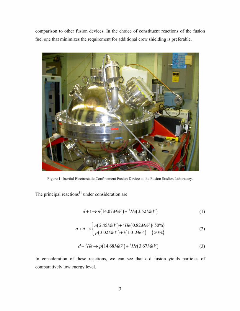
leave the core without losing energy to the plasma. Figure 1 below shows a typical
Inertial Electrostatic Confinement Fusion experimental device located in the Fusion
Studies Lab at the University of Illinois Urbana-Champaign.
Finally for spacecraft applications, thin chamber walls of a space-borne IEC due to the
vacuum of space ensure a lighter structural weight that enables higher payloads in
3
comparison to other fusion devices. In the choice of constituent reactions of the fusion
fuel one that minimizes the requirement for additional crew shielding is preferable.
Figure 1: Inertial Electrostatic Confinement Fusion Device at the Fusion Studies Laboratory.
The principal reactions11 under consideration are
( ) ( )414.07 3.52d t n MeV He MeV+ → + (1)
( ) ( ){ }( ) ( ) { }
32.45 0.82 50%3.02 1.01 50%
n MeV He MeVd d
p MeV t MeV⎧ +⎪+ → ⎨ +⎪⎩
(2)
( ) ( )3 414.68 3.67d He p MeV He MeV+ → + (3) In consideration of these reactions, we can see that d-d fusion yields particles of
comparatively low energy level.

4
The second reaction of d-t fusion has a number of drawbacks.12 Tritium is a radioactive
element that will contaminate isotope separation and other subsystems of the fuel cycle. It
also requires substantial radiation protection measures. It releases a very energetic
neutron that would substantially increase the amount of crew shielding necessary if it was
to be used for spacecraft power or propulsion. Additionally, a special loop would be
required to reproduce tritium adding further weight because of its decay rate. Finally,
there is no adequate method of harnessing the energy of the 14.1 MeV neutron from the
d-t reaction.
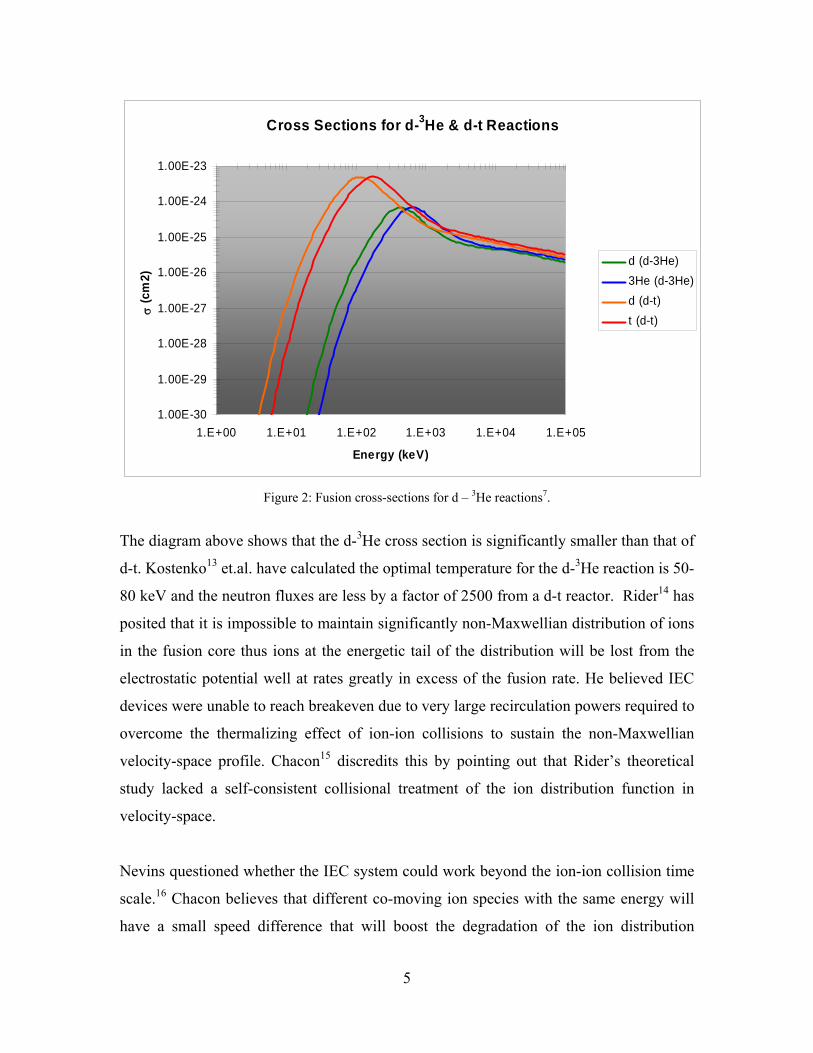
Figure 2 below compares the fusion cross sections for the various reactions under
consideration for the converter-collimator. Equation (3) above also has its challenges. At
50 keV the ratio d-t to d-3He of reaction rates is 14 and at 100 keV the ratio is 5. Thus
both of the d-d fusion branches should be considered in general analysis. Nevertheless the
branches of the d-d burn occur at factors lower than d-3He and thus neutron fluxes are
significantly lower reducing the shielding requirement. Another drawback is the lack of
terrestrial 3He which would require either lunar mining or energy intensive breeding. On
the plus side, d-3He releases a very energetic proton that can be used for direct energy
conversion or possibly direct propulsion.
5
Figure 2: Fusion cross-sections for d – 3He reactions7.
The diagram above shows that the d-3He cross section is significantly smaller than that of
d-t. Kostenko13 et.al. have calculated the optimal temperature for the d-3He reaction is 50-
80 keV and the neutron fluxes are less by a factor of 2500 from a d-t reactor. Rider14 has
posited that it is impossible to maintain significantly non-Maxwellian distribution of ions
in the fusion core thus ions at the energetic tail of the distribution will be lost from the
electrostatic potential well at rates greatly in excess of the fusion rate. He believed IEC
devices were unable to reach breakeven due to very large recirculation powers required to
overcome the thermalizing effect of ion-ion collisions to sustain the non-Maxwellian
velocity-space profile. Chacon15 discredits this by pointing out that Rider’s theoretical
study lacked a self-consistent collisional treatment of the ion distribution function in
velocity-space.
Nevins questioned whether the IEC system could work beyond the ion-ion collision time
scale.16 Chacon believes that different co-moving ion species with the same energy will
have a small speed difference that will boost the degradation of the ion distribution
Cross Sections for d-3He & d-t Reactions
1.00E-30
1.00E-29
1.00E-28
1.00E-27
1.00E-26
1.00E-25
1.00E-24
1.00E-23
1.E+00 1.E+01 1.E+02 1.E+03 1.E+04 1.E+05
Energy (keV)
σ (c
m2)
d (d-3He)3He (d-3He)d (d-t)t (d-t)

6
function and that a more realistic scenario would consider a more homogenous speed
within the ion beam.
Dawson feels that self-burning of advanced fuels at high temperatures is not practical
because Bremsstrahlung losses may exceed the fusion power generated.17 Nevertheless,
Miley18 believes that the β2Β4 scaling of the power density can compensate for these
limitations because the IEC has operating regimes which are non-Maxwellian in nature.
Furthermore, Son and Fisch have shown19 in Fermi degenerate plasmas, the reduction of
ion-electron (i-e) collisions allows the ion temperature to exceed the electron temperature
and reduces Bremsstrahlung losses. They further demonstrate that the fusion ignition
regime is several times larger than previously calculated when accounting for previously
ignored effects or partial degeneracy and relativistic effects on i-e collisions.

7
1.2 Application to Spacecraft Power & Propulsion
A d-3He IEC fusion reactor is the optimum for spacecraft application as all reactants are
charged particles that are idea for direct energy conversion. Of particular importance are
the highly energetic protons and lack of neutron generation resulting in reduced crew
shielding requirements. The IEC acts as a light bulb, creating an isotropic source of
energetic fusion products therefore an efficient way of redirecting them into a collimated
beam, like a flashlight, is needed where they can more easily be used for power
extraction and/or thrust.
One of the conventional methods of collimating charged particles is by applying a
magnetic channel around the particle source. Charged particles are trapped by and move
along lines of magnetic flux. By introducing gradually expanding lines of flux along the
magnetic channel, the perpendicular velocity component is transferred to the parallel one.
The IEC core however, operates in a region of null magnetic field. In order to meet this
requirement Momota and Miley5 proposed a collimator-converter system that uses
utilizes a pair of coils anti-parallel to the magnetic channel to eliminate the field in the
region of the IEC fusion core. This creates a magnetic hexapole configuration with a
vanishing magnetic field at the central domain while leaving a strong magnetic field
outside the coil pair. Figure 3 details the proposed concept of collimating IEC fusion
products from the core at the center, where the rose bars represent the solenoid coil that
generates the magnetic channel, the blue coils generate the magnetic hexapole region, and
the light blue coil represents the stabilization coil to balance the magnetic forces reducing
structural requirements.

8
Figure 3: The proposed magnetic coil configuration used to redirect the isotropic fusion products from the IEC core into a collimated flow along the magnetic channel.
Figure 4 shows the power source configuration using neutral beam injectors as drivers for
the IEC core and the magnetic coil placement with the rose representing the solenoid
coils, the blue representing the floating coils, and the orange representing the stabilization
coils.
Solenoid coils
Floating coils
Stabilization coil
IEC Core

9
Figure 4: Details the composite neutral beam injector IEC with collimator coils for a proposed spacecraft propulsion/power system
The resultant flow of collimated charged particles would be directed into a traveling
wave direct energy converter (TWDEC) shown in Figure 5 below. The device consists of
solenoid coils creating the magnetic channel, an array of modulator grids shown in red,
and an array of decelerator grids shown in blue. A blow-up view of the grid cross-section
is also shown in the figure.
Leaking unburned fuel components would be removed with a magnetic separator at the
entrance of the direct energy converter and pumped out for further refueling. The
TWDEC is composed of an array of metallix meshed grids, which are each connected to
a terminal with an external transmission circuit. The transmission line couples to the
direct energy converter. The number density of fusion protons indicates that the lifetime
Floating coils

10
of a metallic structure submersed into the proton stream could be more than a hundred
years due to sputtering. Momota’s TWDEC overcomes the voltage breakdown limitations
of electrode plate direct energy convertors by using a grid mesh to form a series of
electrodes. The modulator section of the TWDEC is used to modify the beam’s
distribution function to eliminate an oscillating electric field downstream and completes
the proton bunching at the entrance of the decelerator portion of the converter.
Figure 5: Traveling Wave Direct Energy Converter
The decelerator acts as the inverse of a linear accelerator, which converts electric energy
into charged particle kinetic energy by choosing the relative phase between a traveling
wave and charged particles. More detailed studies of the TWDEC have been undertaken
by Momota, Shu, and Ishikawa as previously mentioned. The composite TWDEC with
magnetic expander and magnetic separator is shown in Figure 6. The green dots at the
exit of the TWDEC are electron emitters used to neutralize the particle beam in order to
eliminate charge buildup of the space vehicle.

11
Figure 6: Composite magnetic expander (ME), magnetic separator (MS), and traveling wave direct energy converter (TWDEC) configuration.
Putting all these components together yields the basis of a potential advanced spacecraft
propulsion and power system as shown in Figure 7. Increased power levels are
accomplished by placing the IECs in series and exhausted into the TWDECs. This
configuration minimizes the magnetic field needed by eliminating the need for a
magnetic mirror to reflect the 14.7 MeV protons back toward a single TWDEC.
Figure 7: Proposed spacecraft propulsion and power system utilizing neutral beam injection IEC fusion devices and traveling wave direct energy converters.
ME
MS
TWDEC

12
1.3 Application of Fusion System to Prospective Spacecraft Designs
At the 2002 Space Technology and Applications International Forum, Momota20 et al,
proposed using a series of D-3He fusion reactors in conjunction with magnetic-field
collimation to direct high energy protons into a high-efficiency traveling-wave direct
energy converter system that could be used for spacecraft power system. Using these
parameters, Burton21 outlined a 500MT spacecraft for a manned Jupiter mission using
Krypton ion engines.
Figure 8: Depiction of the Fusion Vehicle Proposed at STAIF 2002.
The following year an updated 300 meter ship design was unveiled at STAIF 200322 that
used 10 IECs serially with an assumed a reactor gain of 9 generating 1394 MW of 14.7
MeV protons, and utilized traveling wave direct energy converters to power the ion
thrusters. Another change was the integration of a magnetic channel semi-circle instead
of a magnetic mirror. This proposed design reduced the transit time to 362 days to Jupiter

13
and back. Once again it is the collimation of these protons that are of interest to this
research.
Figure 9: Depiction of Fusion Ship II from STAIF 2003.
1.4 Research Objectives & Scientific Relevance
The objective of this thesis research was to show that there is a feasible technological
pathway to take isotropically emitted protons from an IEC fusion core and efficiently
guide them into the Traveling Wave Direct Energy Converter. Experimental study of the
specific magnetic field configuration to confine, or collimate, high-energy fusion protons
for possible energy extraction from an inertial electrostatic fusion reactor to provide
either direct thrust or be used as a power source for spacecraft propulsion demonstrates
relevance to the scientific and engineering community.

14
The specific technical objectives of this work encompass the following:
• Describe the theory behind the proposed proton collimation device
• Present the ratios used to reduce a full-size proton collimator to a laboratory
scaled electron collimator simulator
• Describe the design and construction experimental apparatus components,
including the magnetic coils, electron sources, and measurement devices.
• Describe the theoretical and experimental characterization of the electron sources
• Demonstrate the presence of the null magnetic field at the simulated fusion core.
• Present the experimental collimation results for cases with and without a
stabilization coil present.
• Present the scattering results for the case of incoming electrons from an adjacent
device.
• Characterize the energy spectra of the collimated electrons
• Present the experimental collimator efficiency for various magnetic field strengths
and electron source energies.
• Present the findings of a detailed particle computer simulation.
• Compare the computer generated results with those of the experimental apparatus.

15
Chapter 2 Proton Collimation
2.1 Theoretical Description of the Proton Collimator From the starting point of an inertial electrostatic confinement fusion device with
deuterium and helium three fuels, the fusion product of interest will be 14.7 MeV
protons. A collisionless charged particle in an axially symmetric magnetic field will
conserve its Hamiltonian H, and the canonical angular momentum Pθ.. Thus the following
inequality defines the velocity components,
( ) ( )2
2
1 , , 02 2
qH P r z q r zMr θ ψ ϕ
π⎛ ⎞− − − ≥⎜ ⎟⎝ ⎠
(4)
where ( ),r zψ is the magnetic flux and ( ),r zϕ is the scalar potential in cylindrical
coordinates. The region where this inequality is satisfied, known as the “accessible
region” is where the particle is restricted. In a spherical inertial electrostatic confinement
device any charged particles, such as unburned fuel ions, fusion products and electrons
will be located near the origin of the spherical device, thus the canonical angular
momentum of these charged particles will vanish in an IEC. The scalar potential can also
be ignored at a point distant from the IEC region.
From Biot Savart law23 the differential magnetic field dB generated by an infinitesimal
element of the curve ds is
(5)
where d is a vector from the differential current element position, s, to the point r where
the magnetic field is calculated, therefore,
= −d s r (6)
034
Iμπ
×=
ds ddBd

16
Using properties of symmetry and converting to cylindrical coordinates the magnetic
field from a current loop can be expressed as24
( ) ( ) ( ) ( ) ( )( ) ( )
( )2 2
12 202 2
1 / /1 / / sin sin
2 1 / /c c
z c cc c c
r R z RIB r R z R K ER r R z R
μ θ θπ
− ⎡ ⎤− −⎡ ⎤ ⎢ ⎥= − + + +⎣ ⎦ ⎢ ⎥− +⎡ ⎤⎣ ⎦⎣ ⎦ (7)
( ) ( ) ( ) ( ) ( )( ) ( )
( )2 2
12 202 2
1 / /1 / / sin sin
2 1 / /c c
r c cc c c
r R z RI rB r R z R K ER z r R z R
μ θ θπ
− ⎡ ⎤− −⎛ ⎞ ⎡ ⎤ ⎢ ⎥= − + + − +⎜ ⎟ ⎣ ⎦ ⎢ ⎥⎝ ⎠ − +⎡ ⎤⎣ ⎦⎣ ⎦
(8)
where K and E are elliptical integrals of the first and second kind respectively, and the
elliptic functions argument sin θ is given by,
( )( ) ( )
1/2
2 2
4 /sin
1 / /c
c c
r R
r R z Rθ
⎡ ⎤⎢ ⎥=⎢ ⎥+ +⎡ ⎤⎣ ⎦⎣ ⎦
(9)
A representative accessible region can be created by a pair of magnetic coils installed
anti-parallel to a uniform magnetic field. Figure 10 shows the magnetic field created by a
pair of Helmholtz coils that could be used in a magnetic channel to create a null field
suitable for an IEC fusion core.

17
Figure 10: Helmholtz coil generated magnetic field showing null field region at origin.
A central null field is critical to optimum operation of an inertial electrostatic fusion
device as the presence of magnetic field will perturb the particle trajectories and create an
off-core density peak resulting in a reduced fusion reaction rate.24,Coil currents are
chosen so that the magnetic field at the center will be null. When the center of the
cathode grid is placed along the chamber axis, the current per unit length, NI, on the
external solenoid must be equivalent to the current on each internal Helmholtz coil in
order to cancel the magnetic field at the cathode grid. A favorable configuration utilizes
two “Helmholtz Coils,” where the spacing of the coils is equal to the coil radius, thus
providing a wide region with a vanishing magnetic field. The coil current can be chosen
to achieve this isolation of the accessible region from both the chamber wall and the coil.
2sin
C
NII
φρ
= (10)
The ratio of solenoid current to floating coil current necessary to create a central null
field as well as the optimum spacing and radius of the coils in Equation 10 was developed

18
by Nieto24. Here, NI is the Ampere-Turns of the solenoid coil, IC is the current of the
floating coils, φ is the angle between the chamber centerline and the coil from the axis of
floating coil symmetry, ρ is the distance from the centerline to the floating coil shown in
Figure 11. In that work, ρ = 1, and φ = π/2 were determined as the optimum settings.
Figure 11: Illustration of geometric parameters for coil configuration studies
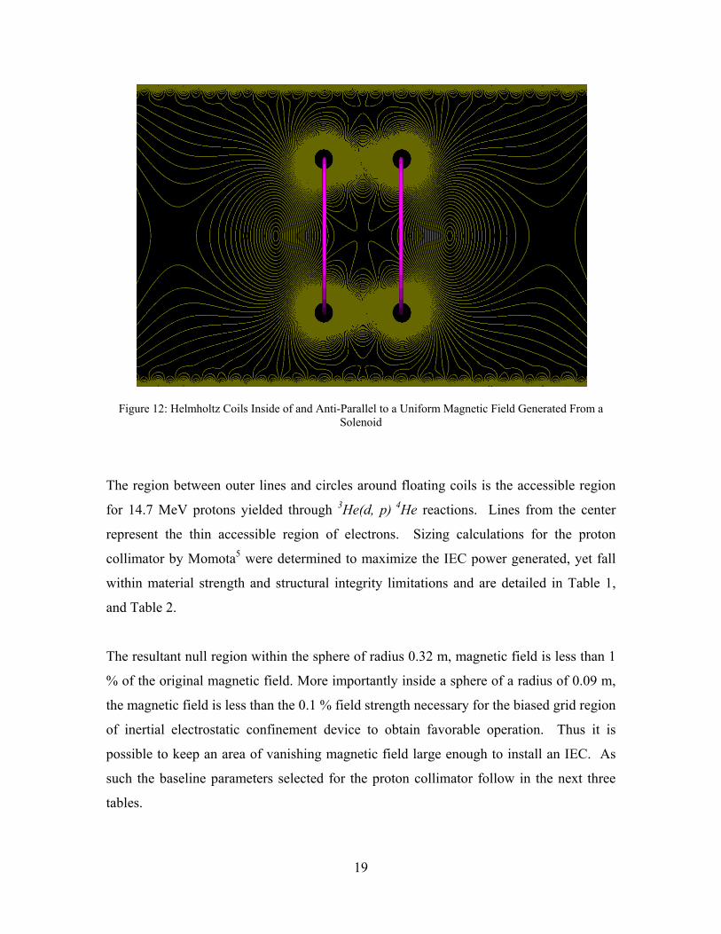
Figure 12 shows the resultant hexapole magnetic field described by Momota and the null
field center created when a pair of anti-parallel Helmholtz coils is inserted into a uniform
magnetic field created by a solenoid.
19
Figure 12: Helmholtz Coils Inside of and Anti-Parallel to a Uniform Magnetic Field Generated From a Solenoid
The region between outer lines and circles around floating coils is the accessible region
for 14.7 MeV protons yielded through 3He(d, p) 4He reactions. Lines from the center
represent the thin accessible region of electrons. Sizing calculations for the proton
collimator by Momota5 were determined to maximize the IEC power generated, yet fall
within material strength and structural integrity limitations and are detailed in Table 1,
and Table 2.
The resultant null region within the sphere of radius 0.32 m, magnetic field is less than 1
% of the original magnetic field. More importantly inside a sphere of a radius of 0.09 m,
the magnetic field is less than the 0.1 % field strength necessary for the biased grid region
of inertial electrostatic confinement device to obtain favorable operation. Thus it is
possible to keep an area of vanishing magnetic field large enough to install an IEC. As
such the baseline parameters selected for the proton collimator follow in the next three
tables.

20
Table 1: Floating (Helmholtz) Coil Parameters for Proton Collimator
Major Radius 1. 5 m
Cross Section π × 0. 0752 m2
Current -2. 25 MAT
Conductor He-II cooled Nb3SnO4
Axial Position ± 0. 75 m
Table 2: Solenoid Coil Parameters for Proton Collimator
Inner Radius 2. 1 m
Current/Length 0. 76213 MAT/m
Magnetic Field 0. 9577 T
Stability analysis by Momota25 further suggests the Helmholtz coils are stable against
axial and tilt perturbations, yet weakly unstable to a shift force perpendicular to the axis.
If the coil shifts vertically from its equilibrium position by a distance of only 1 mm, the
resulting force acting on a floating coil is 3.85×10³ N under the assumption of a 1.5 meter
radius Helmholtz coil with 25 MAT. Minor structural support from thin pipes for current
and coolant feed sufficient offset the week displacement. Thus in view of practical
applications, it is possible to ignore the instability of vertical modes in the present
experiment. For example, three pipes connected to the coil, one for current feed and the
other two for coolant recycling, are capable of supporting this force provided that each
pipe is made of conventional materials with a stress of 30 kg (w)/mm2 and has 5 mm outer
radius and 0.5 mm thickness. The increased cross-sectional size of the cathode to
accommodate cooling results in a lower transparency and thus reduced fusion core
efficiency. However, bombardment loss of particles onto the cathode structure coolant
pipes is estimated to be less than 0.36 %.

21
Figure 13: Accessible region in center produced by a pair of Helmholtz coils (purple) and an anti-parallel stabilization coil (red) is isolated from both the vacuum chamber and the magnetic coils. The region
between the outer lines and circles is the proton accessible region.
Under consideration of the collimator sizing Momota observed that an attractive force
between the Helmholtz coils on the order of 106 Newtons would be generated if the coil
current is on the order of a mega-amp-turn for a coil major radius of a few meters
necessary for structural integrity. The adequate supporting structure would disturb the
positive field characteristics so a corrugated magnetic channel is created by installing a
canceling coil anti-parallel to the Helmholtz coil configuration. Due to the additional coil,
the area of null-magnetic field near the center decreases to 75 % of the original without
the anti-parallel stabilization coil. This result can be seen visually by comparing the null
regions between Figure 12 and Figure 13 above.

22
Table 3: Stabilization Coil Parameters for Proton Collimator
Major Radius ± 1. 5 m
Cross Section ×π 0. 0442 m2
Current 0. 7811 MAT
Conductor He-II cooled Nb3SnO4
Axial Position 0 m
2.2 Scaling from a Proton Device to an Electron Simulation It is possible to study the essential characteristics of proton collimator by building an
electron scale simulation device with adjustments for the charge/mass ratio. Because the
proton is the most energetic particle in the d-3He reaction, confinement of the proton also
implies confinement of the other fusion products and fuels. For the electron simulator
device, we will further simplify by focusing solely on the protons, by proxy, the
electrons, and ignore the remaining particles. As such to study the essential
characteristics of the collimator experimentally, a scaling relation was developed related
to the accessibility region deemed the “accessibility index” defined by
( ) ( ) 2
2
,1, ; ,2
P q r zK r z W P
W Mrϕ
ϕ
⎡ ⎤− Ψ⎣ ⎦≡ (11)
where W is the energy of the particle under consideration. If the value is identical in
respective collimators, then the contour of the accessible region relative to the coils and
the wall will also be the same. The simplest experiment to undertake would be to
simulate protons with electrons. The scaling ratio defined25 by
electronfloatingprotonfloating
RR
η = (12)
and is the ratio of the electron device to the proton device. This relation can be extended
to the current by

23
pp
epc
ec WM
mWII = (13)
where ecI is the current on the floating coil of the electron collimator and We is the
electron energy. Nieto believes that once this relation is satisfied, the electron dynamics
in the electron collimator is analogous to that of protons in the proton collimator.
The electron energy selected for the experiment was 300 eV. The scale factor however,
changes the current density on a coil according to the relation by Nieto24
2
1ee p
p p
mWj jM W η
= × (14)
The quantities je and jp are the current densities in an electron and proton collimator
respectively, thus a small value of η requires a higher current density on a floating coil in
the electron collimator.
Given these relations the scale between the collimators used for the experiment are
summarized in the following two tables.
Table 4: Floating Coil Scaling Relations
Radius of Floating Coil
Cross-Section of Floating Coil
Current on the Floating Coil
Proton Collimator 1.5 m 75 mm 2.25 MAT
Electron Collimator 0.15 m 7.5 mm 234.9 AT
Note that the current density of the floating coils is as small as 1.33 A/mm2, allowing
natural cooling of the coils via heat conduction through the current feeding wires and coil
supporters in the electron collimator simulator. An adhesive problem in construction of

24
the coils however prevented long run times due to off-gassing and subsequent pressure
increases in the experiment.
Table 5: Stabilization Coil and Solenoid Coil Scaling relations
Stabilization Coil Current Solenoid Current Particle Energy
Proton Collimator 0.78 MAT 0.762 MAT/m 15 MeV
Electron Collimator 81 AT 79.55 AT over 1 m 300 eV
Thus it is feasible to construct an electron collimator simulator as a surrogate to validate
the proton collimator concept. The application of these device parameters obtains an
electron accessible region in the electron collimator quite similar to the proton accessible
region in the proton collimator. Consequently, one observes collimated electron flux
along the magnetic channel of the electron collimator similar to proton flux in the proton
collimator.
Based on these calculations an experimental vacuum chamber and test apparatus was
designed to study the electron transport characteristics within a magnetic collimator
system that can accurate simulate the proton flux from a d-3He inertial electrostatic fusion
device. Figure 14 illustrates the calculated magnetic field lines using the electron
collimator scaled parameters of Table 4 for the floating coils and Table 5 for the
stabilization coil and the solenoid coils in their proper physical configuration. Figure 15
illustrates the calculated equivalent magnetic vector potential obtained for the electron
collimator simulator from the same tables. The specific design parameters of the
constructed vacuum chamber and the magnetic coil experimental components are detailed
in the next chapter.

25
Figure 14: Magnetic field flux composite for experimental device.
Figure 15: Magnetic vector potential A

26
Chapter 3 Experiment Device Configuration
3.1 Vacuum Chamber
The preliminary design for the vacuum chamber was taken from the original proposal. It
was decided that a two meter version better suited the present and future project needs. A
CAD drawing of the vacuum chamber is shown in Figure 16. Requirements for the
chamber follow. 1. Two CF100 (ConFlat, copper gasket) flanges mounted in opposition to support up
to two Alcatel ATP150 turbopumps (all CF flanges are rated to 1x10-13 Torr)
2. One CF200 flange bottom mounted to accommodate Alcatel ATP900 turbopump
3. Two 21 1/8″ wire seal flanges at both ends of the chamber rated to 1x10-13 Torr to provide access for installing inner structure. Other design features of the wire seal end flanges are:
a. Equipped with 12″ CF reducer flanges, to reduce cost of repeated chamber entry
b.Four 2 ¾″ CF flanges at 90o intervals outside the 12″ CF for viewing inner structure and to serve as feedthrough ports.
4. Twelve 2 ¾″ CF ports at 90o intervals at 0.5 m, 1.0 m, and 1.5 m stations for
additional viewports and feedthroughs.
5. 16 inner support loops to mount support rods for inner structure positioning.
6. Electropolished 316 low-carbon stainless steel, to minimize outgassing.

27
Figure 16 CAD drawing of UHV chamber.
Pressure was monitored by a thermocouple for high pressures (>1 mTorr), and an
ionization gauge tube near the turbopump end of the chamber for low pressures (<1
mTorr). The roughing pump was a Kurt Lesker model 100-3-5, and the turbopump was
an Alcatel ATP-150.
Power supplies for the field-generating components of the experiment were as follows
a. 3 30VDC, 6A Tenma supplies for stabilization and solenoidal coils
b. 1 80VDC, 8A Kepco supply for the outer chamber coils.
c. 2 2000VDC 20mA supplies for filament and extraction grid biasing.
Three 1-inch square rods supported the outer coils in their proper position. Axial spacing
of the coils was provided by sequential grooves cut into the rods. The radial centering of
the coils was provided by the support rods as well. Figure 17 shows the outer coils, their
support rods and the unistrut support frame. The power supplies were mounted at the

28
bottom of the test stand (not visible in figure.) Measurements were conducted with a
gaussmeter to verify that neither the chamber not the test stand significantly perturbed the
desired magnetic field characteristics inside the chamber.
Figure 17 Vacuum Chamber Exterior with Solenoidal Coils.
An argon venting system was installed on the chamber stand structure to reduce chamber
pump down time. The argon pressurizes the chamber and creates a positive flow of gas
out of the chamber to minimize contamination from the atmosphere when the chamber is
opened for servicing. The Argon gas-feed system also serves as a supply of gas for
discharge cleaning the chamber and other internal surfaces. As previously mentioned the
chamber was constructed of 316 low-carbon stainless steel to provide an ultra high
vacuum system for a low leak rate necessary with this size of chamber that would be free
of contaminants and most similar to that encountered in interplanetary space on the order
of 10-6 Torr and lower.
Unistrut Test
Stand
Argon Venting System
Solenoid Coils
Support Rods
Chamber Supports

29
Figure 18: Chamber dimensions – diameters
Figure 19: Chamber dimensions - angles

30
3.2 Solenoidal Coils Each solenoidal coil has four layers with six turns in each layer (24 turns per coil). The
wire used for making the solenoid coils was 2-mm diameter, circular cross section
insulator coated magnet wire. The Teflon bobbin used to construct the coils had a 600
mm and a removable outer housing to allow for easy removal of the finished coil
structure. The wire spool was mounted on another shaft, with a friction housing that
provided adequate tension necessary for the coil winding process. After completing each
6-turn layer, Epoxy was applied to adhere the layer to itself and allowed to dry in order to
provide a firm base for the next layer of winding. This process is repeated for each of the
four layers.
(a) (b)
Figure 20: Section view of solenoid coil, (a) 3-dimensional cut view, (b) cross section of solenoid coil.
The design requirements of the solenoid coil mounting structure are the following:
• The center of solenoid coil should be on the axis of vacuum vessel.
• The side areas of the solenoid coils should be perpendicular to the axis of vacuum
vessel.
• Each solenoid coil should be equidistant from its neighboring coil.
• The position of each solenoid coil should be fixed even under application of
magnetic field stresses.
• The center of solenoid coil array should be the same as that of Helmholtz
(floating) coil.

31
The above requirements were achieved through the fabrication of 1″ square cross section
wooden support rods with grooves cut along their length, as shown in Figure 21. The
width of each groove was the same as that of solenoid coil, or 15 mm. The distance
between each groove was 35 mm, and there were a total of 20 grooves, one for each coil.
Figure 21 also details how the coils fit into the wooden support rods. After placing the
solenoidal coil array around the vacuum chamber and mounting the array onto the
support rod grooves, the coil assembly is radially centered and fixed in position with
wooden shims. The wooden shims were suitably resistant to the heat generated by the
coil array during intense operation.
Figure 21: Diagram of solenoid coil support rod (left) and the solenoidal coil assembly (right).
3.3 Floating Coils The design parameters for the floating and stabilization coils for the electron-collimator
are detailed in Table 6. The scaling relations that allow comparison of the electron
collimator to a fusion-proton collimator are discussed in the previous section. The
construction and installation techniques of the inner coils are detailed below.
32
Table 6: Physical Parameters of the Electron Collimator Coils
Parameter Floating Coils Stabilization Coil Major Radius 0.15±0.01m 0.15±0.01m Minor Radius 15±1mm 10±1mm Cross Section π x 152mm2 π x 102mm2
Current 1.175A(300V)/1.435A(450V) 1.03(300V)/1.26A(450V)
Conductor Copper Copper
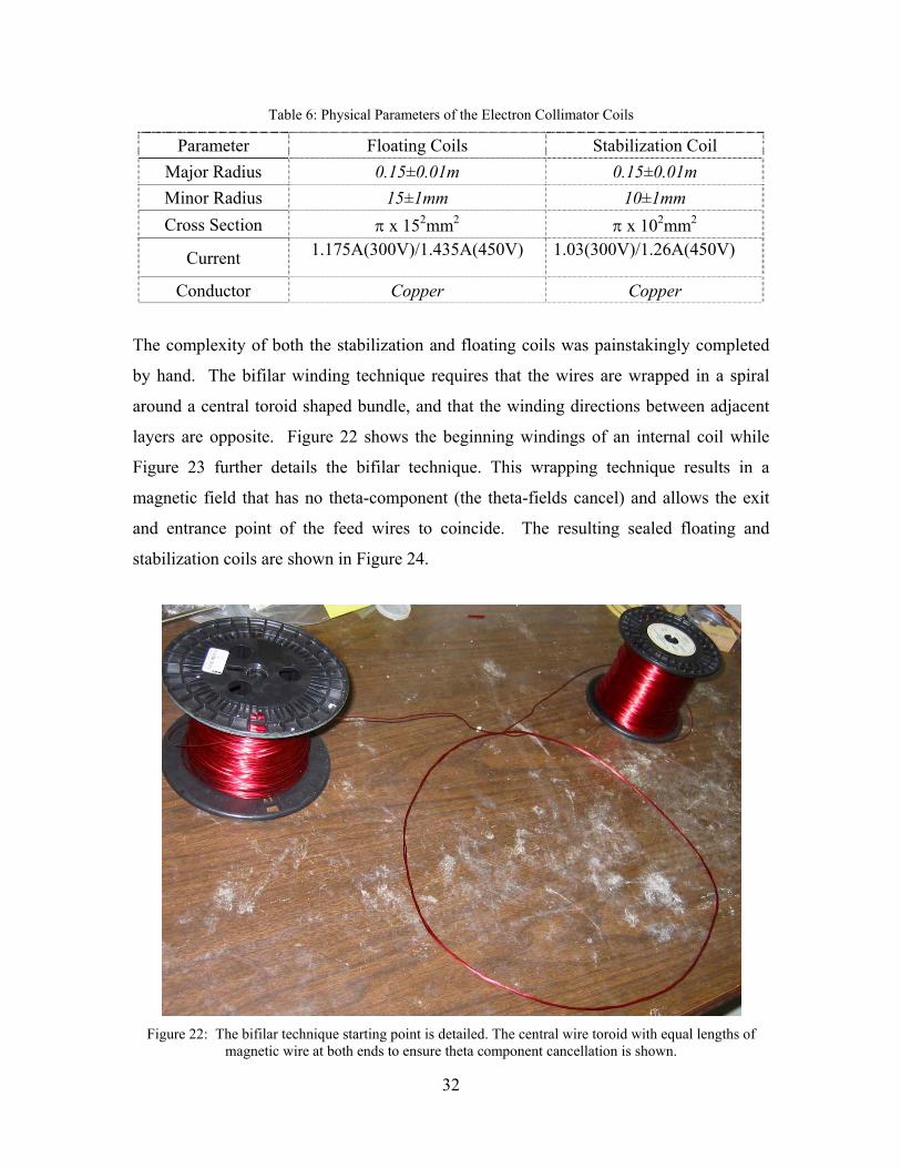
The complexity of both the stabilization and floating coils was painstakingly completed
by hand. The bifilar winding technique requires that the wires are wrapped in a spiral
around a central toroid shaped bundle, and that the winding directions between adjacent
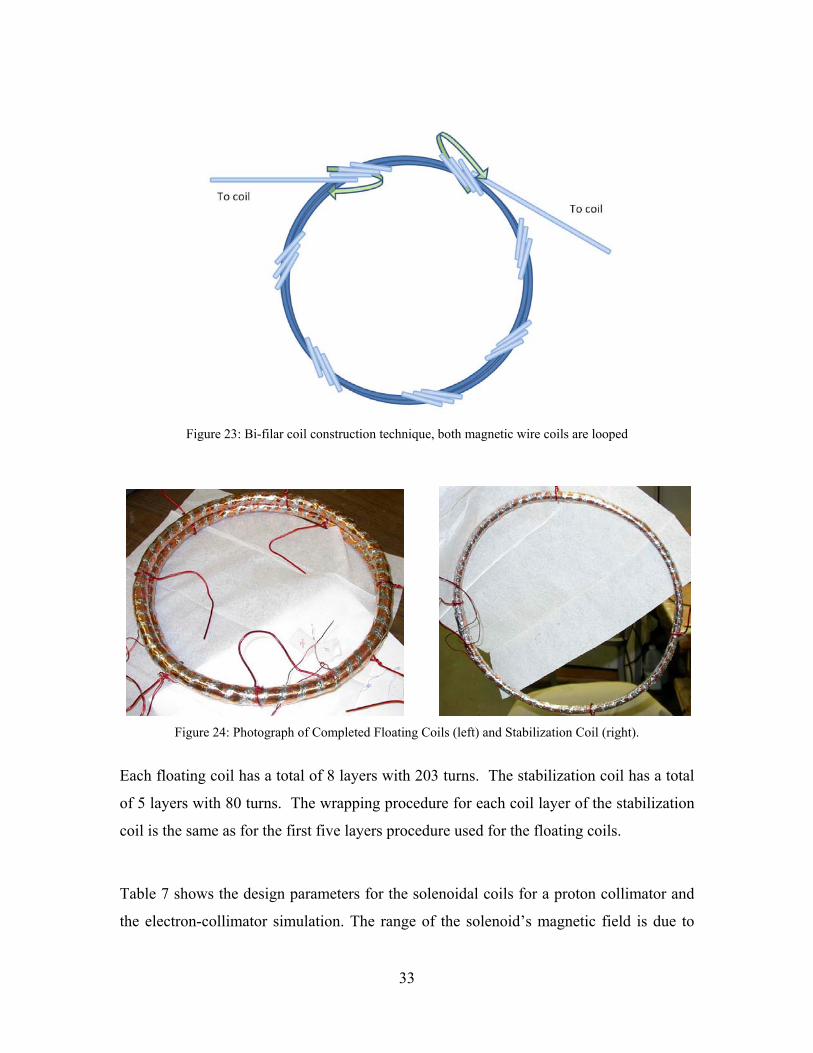
layers are opposite. Figure 22 shows the beginning windings of an internal coil while
Figure 23 further details the bifilar technique. This wrapping technique results in a
magnetic field that has no theta-component (the theta-fields cancel) and allows the exit
and entrance point of the feed wires to coincide. The resulting sealed floating and
stabilization coils are shown in Figure 24.
Figure 22: The bifilar technique starting point is detailed. The central wire toroid with equal lengths of
magnetic wire at both ends to ensure theta component cancellation is shown.
33
Figure 23: Bi-filar coil construction technique, both magnetic wire coils are looped
Figure 24: Photograph of Completed Floating Coils (left) and Stabilization Coil (right).
Each floating coil has a total of 8 layers with 203 turns. The stabilization coil has a total
of 5 layers with 80 turns. The wrapping procedure for each coil layer of the stabilization
coil is the same as for the first five layers procedure used for the floating coils.
Table 7 shows the design parameters for the solenoidal coils for a proton collimator and
the electron-collimator simulation. The range of the solenoid’s magnetic field is due to

34
the fact that the solenoid is finite. The value of 3.3X10⁻⁶ T corresponds to the center of
the solenoid field while the value 0.8X10⁻⁶ T corresponds to the edge of the solenoid. In
the experiment, the collector plates are located 20 cm from the end of the solenoid which
corresponds to a magnetic field of 1.32X10⁻⁶ T. This represents about 4% of the peak
magnetic field generated at the center of the device. The effects will be addressed later.
Table 7: Design Parameter Comparison for the Solenoidal Coil
Parameters Proton Collimator Electron Collimator Inner Radius 2.1 m 0.3 m
Current/Length 0.762 MAT/m 1.417 AT/m Magnetic field 0.9577 T 0.8 -3.3X10⁻⁶ T
Figure 25 details the physical dimensions of the internal coil configuration and its
relation to the electron source as determined by Nieto.24 The construction and installation
techniques of the outer coils are discussed below.
Figure 25: Internal Coil Geometry of Floating Coils (Purple), Stabilization Coil (Pink), & Electron Source at the origin (white)

35
Both the stabilization and floating coils are approximately 30 cm in diameter; although
inner and outer dimensions differ depending on the number of layers in the coil (the
stabilization coil is narrower as it has significantly fewer turns). The coils are installed in
the chamber using copper wire tied to the internal support rods in a similar manner to the
collector plates as shown in Figure 26 and Figure 27. The coils are radially centered
within the vacuum chamber and axially centered relative to the outer solenoid coils. The
support and power feed system for the electron source was placed in two separate
configurations. For radial emission testing, the stabilization coil was moved off-center
and the feed-support system was fed to the chamber center vertically. For normal
operation and testing, the support-feed was mounted horizontally as shown in Figure 26.
Figure 26: Internal layout of electron collimator components with the anode and cathode of the electron source, magnetic coils, collector plates and structural supports. The same figures also show the position of the stainless steel mounting rods which were
used to anchor and support the magnetic coils and the collector plates. Figure 26 shows
the mounting rods at the top and bottom of the chamber from along the axis of symmetry
while Figure 27 shows all four of the mounting rods at symmetric positions to minimize

36
perturbation of the magnetic field. Magnetic coils and collector plates were held in place
on the rods by movable stainless steel circular mounts.
Figure 27: Internal Coil Configuration for the Electron Collimator before Insertion of Electron Source with 1st generation collector plate arrangement
The spacing of the coils depends only on the radial dimensions of the coils themselves.
The stabilization coil is equidistant between the two floating coils. This coincides with
the 0.25-m first station point. Floating coils were spaced axially one half-radius (7.5 cm)
from the stabilization coil on both sides of the stabilization coil (one coil radius between
the two floating coils), as depicted above. The magnetic fields from the floating coils are
in the same direction; however, the magnetic field from the stabilization coil opposes that
of the floating coils. The filament-extractor assembly is centered within the inner coils
where the magnetic field is minimal as shown previously in Figure 26.

37
The inner structure of the chamber uses stainless steel rods and shaft collars to mount the
coils and collector plates. Figure 27 shows the coils, collector plates and support rods
mounted inside of the vacuum chamber. The coils were mounted with a separation of 7.5
cm (one coil radius) between the stabilization coil and the floating coils on both sides of
it. Insulated copper wire allows mounting of the coils and provides ease of adjustment.
The 2 ¾″ CF ports at the 0.5 meter station level were used to provide electrical
connections to the coil power supplies. These stations coincide with the positions of the
coils. Copper-Beryllium (CuBe) power connectors are used to connect coil wire leads to
the electrical vacuum feedthrough.
3.4 Collector Plates
3.4.1 Axial Electron Plates A set of axial collector plates were constructed and inserted into the chamber to measure
the percentage of electrons escaping the confinement region near the radial collector
plates. The axial collectors consist of eight 0.15 m wide ring plates with the same radius
of the internal coils. Four of the plates are placed between the floating coils and the two
other sets each with two plates are placed outsides of the central floating coils. All the
electron collector plates are made of copper. The spacing between the rings is kept
constant. Figure 28 shows a diagram of the axial collector rings relative to the floating
coils and a photograph of the collector rings.
(a) (b)
Figure 28: (a) Diagram of axial collector ring relative positions and (b) the actual collector ring assemblies.

38
3.4.2 Radial Electron Plates The radial collector plates were originally made from copper foil mounted on a Teflon
plate for stability at the one-meter station level. A 2 ¾″ CF port provided a feedthrough
for wiring. The plates are connected to a microammeter outside the chamber. An
improved version which did not use Teflon and has equal-area rings was constructed
from thicker copper plates and was used on the following tests. In addition to these
improvements, the pass-through design of the new collector plate assembly should also
improve gas conductance through the chamber, resulting in lower operating pressures in
the experiment area of the chamber. The Teflon-backed collector plates are shown in
Figure 27 and the improved collector plate design are shown in Figure 29.
Figure 29: Improved Collector Plate Configuration
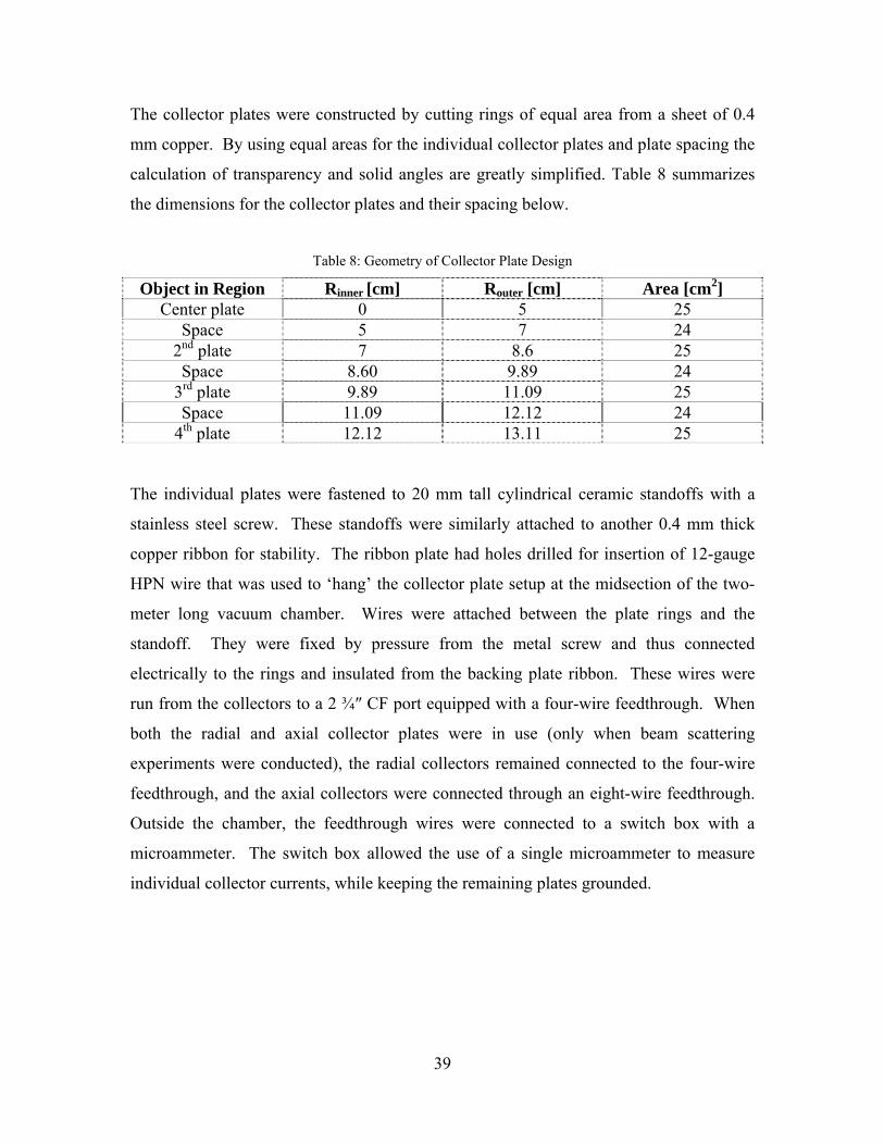
39
The collector plates were constructed by cutting rings of equal area from a sheet of 0.4
mm copper. By using equal areas for the individual collector plates and plate spacing the
calculation of transparency and solid angles are greatly simplified. Table 8 summarizes
the dimensions for the collector plates and their spacing below.
Table 8: Geometry of Collector Plate Design
Object in Region Rinner [cm] Router [cm] Area [cm2] Center plate 0 5 25
Space 5 7 24 2nd plate 7 8.6 25 Space 8.60 9.89 24
3rd plate 9.89 11.09 25 Space 11.09 12.12 24
4th plate 12.12 13.11 25
The individual plates were fastened to 20 mm tall cylindrical ceramic standoffs with a
stainless steel screw. These standoffs were similarly attached to another 0.4 mm thick
copper ribbon for stability. The ribbon plate had holes drilled for insertion of 12-gauge
HPN wire that was used to ‘hang’ the collector plate setup at the midsection of the two-
meter long vacuum chamber. Wires were attached between the plate rings and the
standoff. They were fixed by pressure from the metal screw and thus connected
electrically to the rings and insulated from the backing plate ribbon. These wires were
run from the collectors to a 2 ¾″ CF port equipped with a four-wire feedthrough. When
both the radial and axial collector plates were in use (only when beam scattering
experiments were conducted), the radial collectors remained connected to the four-wire
feedthrough, and the axial collectors were connected through an eight-wire feedthrough.
Outside the chamber, the feedthrough wires were connected to a switch box with a
microammeter. The switch box allowed the use of a single microammeter to measure
individual collector currents, while keeping the remaining plates grounded.

40
3.5 Electron Sources
3.5.1 Spherical In order to simulate the isotropic proton emission from the inertial electrostatic
confinement fusion device, an isotropic electron source was created. The source consisted
of using a tungsten filament biased with an alternating current source of between 10 and
20 mA, and a DC bias between -50 to -300 V. The spherical shaped filament was
centered inside a larger steel wire extraction grid that was biased a near ground potential.
The emitter structure currently consists of a 0.1-mm spherical tungsten filament mounted
at the center of a stainless steel (non-magnetic) cage extraction grid. The leads of the
filament are insulated by ceramic (alumina) tubing and connected to a 15-amp four-prong
nickel-wire 2-¾” CF feedthrough. Steel hose clamps stabilize the insulator tube
configuration. Figure 30 shows the filament-extractor assembly; however, the hose
clamps are not shown here. Figure 31 shows the filament-extractor assembly within the
chamber. The filament is centered within the internal coils.
Figure 30: Filament-Extractor Grid Setup
Insulating Tubes
Nickel Rods
Cu-Be Connector
Tungsten Filament
Extraction Grid
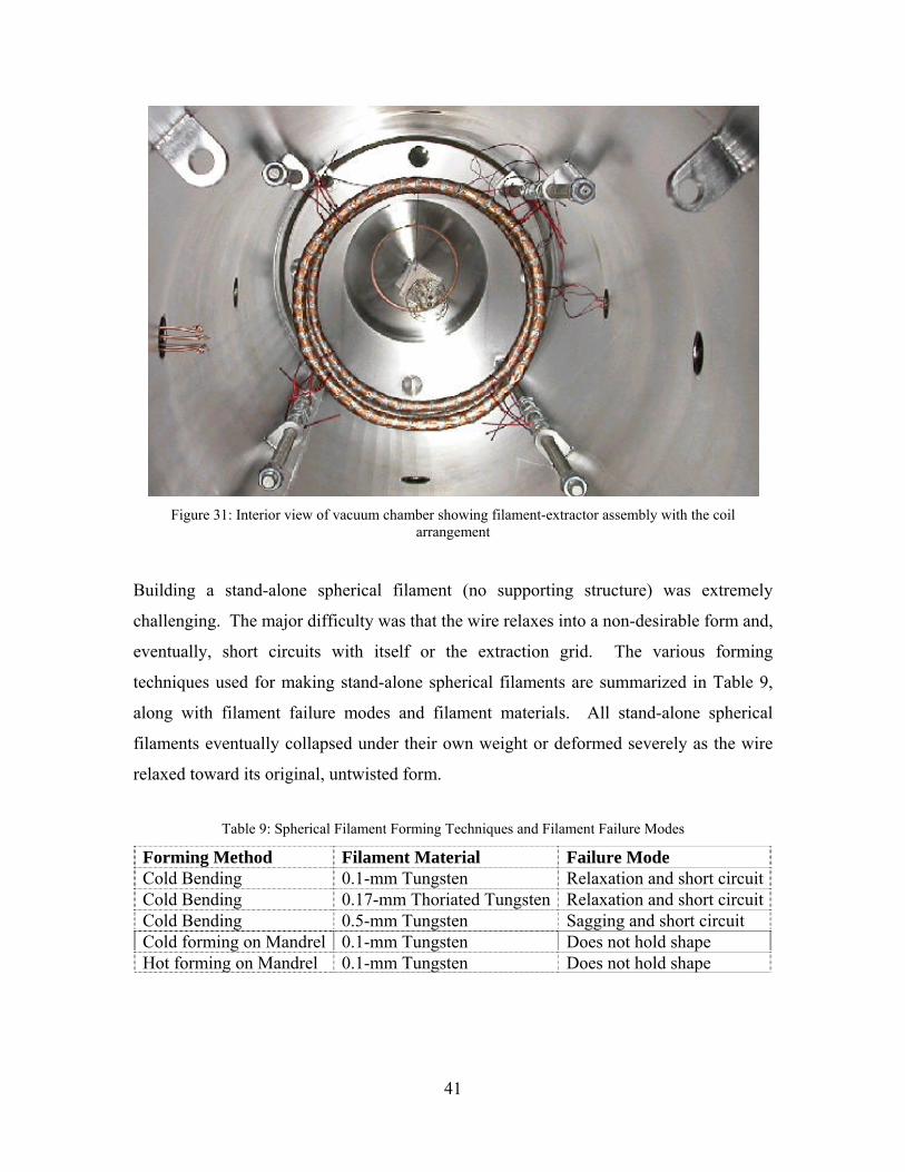
41
Figure 31: Interior view of vacuum chamber showing filament-extractor assembly with the coil
arrangement
Building a stand-alone spherical filament (no supporting structure) was extremely
challenging. The major difficulty was that the wire relaxes into a non-desirable form and,
eventually, short circuits with itself or the extraction grid. The various forming
techniques used for making stand-alone spherical filaments are summarized in Table 9,
along with filament failure modes and filament materials. All stand-alone spherical
filaments eventually collapsed under their own weight or deformed severely as the wire
relaxed toward its original, untwisted form.
Table 9: Spherical Filament Forming Techniques and Filament Failure Modes
Forming Method Filament Material Failure Mode Cold Bending 0.1-mm Tungsten Relaxation and short circuitCold Bending 0.17-mm Thoriated Tungsten Relaxation and short circuitCold Bending 0.5-mm Tungsten Sagging and short circuit Cold forming on Mandrel 0.1-mm Tungsten Does not hold shape Hot forming on Mandrel 0.1-mm Tungsten Does not hold shape

42
Typical lifetimes of these filaments ranged from 5 minutes to 1 hour, depending on the
filament material and operating current (temperature). The 0.17-mm thoriated-tungsten
filament lasted for a few days, probably because the required operating temperature was
lower, but eventually short circuited with itself.
(a) (b)
Figure 32: (a) Spherical Filament (0.1-mm Tungsten) and Support Structure and (b) the Spherical Filament while in use
To prevent filament deformation problems, a filament support structure has been
implemented. The support structure consists of an alumina ring with holes bored around
its circumference to support the filament wires. Figure 32 shows a supported tungsten
filament with 0.1-mm tungsten filament wire. This design has been tested extensively,
and all collimator data presented here used this filament. The alumina sleeve that holds
the support ring also stops electrical short circuits to the extraction grid and allows a
more rigid filament mount with the power feedthrough (see Figure 33: Experiment
spherical filament stabilization and extraction grid concept). This more rigid mount is
achieved by tying the two alumina insulating tubs and the filament support tube together
with a stainless steel hose clamp. This prevents any movement of the alumina tubes,
assuring that a short circuit to the extraction grid does not occur.

43
Figure 33: Experiment spherical filament stabilization and extraction grid concept
It was necessary to test the electron emission uniformity in order to ensure a good
approximation to an isotropic source. For this test the electron source was mounted from
the top of the chamber with a rotatable flange mount. The source insulators and feed
sleeve were shortened in order to reach the axis-symmetric center of the chamber. The
results of this test are shown in Figure 34.

44
0
30
60
90
120
150
180
210
240
270
300
330
0100200300400500600700800900
1000110012001300
0100200300400500600700800900
1000110012001300
Col
lect
or P
late
Cur
rent
[μA
]
plate 1 plate 2 plate 3 plate 4
θ
Figure 34: Study of asymmetrical isotropic electron source on collector plate current
The asymmetry in the electron source measurements can be attributed to many factors.
One contribution is a 2 wire effect of the feedthrough due to independent feeds for the
extraction grid (equivalent to ground) and the spherical filament (negative potential and
AC driven) which was rotated around with the electron source. Another potential source
of the asymmetry can be attributed due to settling of the extraction grid resulting in an
off-center location of the spherical filament. The center plate measurements would seem
to support this as the extraction grid appears to have fallen farther away from one side of
the filament during half of the revolution while the other half was closer to the filament.
Confirmation of this could have been obtained by employing 2 sets of collector plates,
one on each end of the collimator. The third potential source of the asymmetry can be
attributed to the asymmetrical shape of the extraction grid sphere. In order to provide
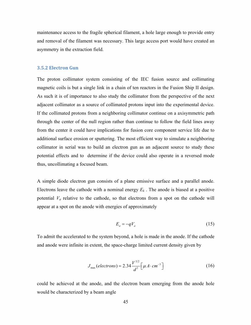
45
maintenance access to the fragile spherical filament, a hole large enough to provide entry
and removal of the filament was necessary. This large access port would have created an
asymmetry in the extraction field.
3.5.2 Electron Gun The proton collimator system consisting of the IEC fusion source and collimating
magnetic coils is but a single link in a chain of ten reactors in the Fusion Ship II design.
As such it is of importance to also study the collimator from the perspective of the next
adjacent collimator as a source of collimated protons input into the experimental device.
If the collimated protons from a neighboring collimator continue on a axisymmetric path
through the center of the null region rather than continue to follow the field lines away
from the center it could have implications for fusion core component service life due to
additional surface erosion or sputtering. The most efficient way to simulate a neighboring
collimator in serial was to build an electron gun as an adjacent source to study these
potential effects and to determine if the device could also operate in a reversed mode
thus, uncollimating a focused beam.
A simple diode electron gun consists of a plane emissive surface and a parallel anode.
Electrons leave the cathode with a nominal energy Ek . The anode is biased at a positive
potential Va relative to the cathode, so that electrons from a spot on the cathode will
appear at a spot on the anode with energies of approximately
a aE qV= − (15) To admit the accelerated to the system beyond, a hole is made in the anode. If the cathode
and anode were infinite in extent, the space-charge limited current density given by
3 2
3max 2( ) 2.34 VJ electrons A cm
dμ −⎡ ⎤= ⋅⎣ ⎦ (16)
could be achieved at the anode, and the electron beam emerging from the anode hole
would be characterized by a beam angle

46
3
ard
α = (17)
where d is the anode-cathode spacing and ra is the radius of the anode hole. Since the
most divergent electron arriving at the anode is emitted parallel to the cathode with
energy Ek , it can be see that the pencil angle characterizing the beam from the anode
aperture would be
k
a
EE
θ = (18)
For a cathode of finite extent, the space-charge interaction causes the beam to spread
laterally within the gap between cathode and anode. Pierce26 has shown that the electric
field in an infinite space charge-limited diode can be reproduced in the region of a finite
cathode by means of a conical cathode structure, shown in Figure 35, offset at 220 where
the maximum current of electrons is
2
2 3/2max max 7.35 [ ]a
a arI r J V Ad
π μ= = (19)
Figure 35: Diagram of Pierce Diode electron gun as described in Building Scientific Apparatus

47
The parameters for the Pierce Diode electron gun constructed for the experiment were
designed to emulate the 300 eV electrons and 20 mA under study from the filament
extractor grid and are detailed in the following table.
Table 10: Pierce Diode Electron Gun Parameters
Maximum Current (Imax) ~20 mA
Electron energy (Va) 200-300 V
Electron Gun Radius (ra) 5 mm
Manufactured Material 314 stainless steel
Anode-Cathode distance (d) 14.5 mm
Spread angle (α) 6.6°
The electron gun consists of a conical cathode and a plate anode is shown in Figure 35. A
0.1 mm diameter tungsten wire filament is positioned in the central bore of the conical
electrode and is heated by an electrical current passing through it. Electrons are emitted
from the filament due to thermal ionic emission.
Using the (X)OOPIC code reproduced in
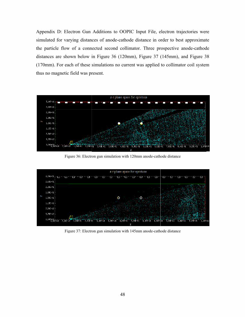
Appe
simul
the p
distan
(170m
thus n
endix D: Ele
lated for var
particle flow
nces are sho
mm). For ea
no magnetic
Fig
Fig
ectron Gun
rying distan
w of a conn
own below i
ach of these
c field was pr
gure 36: Electr
gure 37: Electr
Additions t
nces of anod
nected secon
in Figure 36
simulations
resent.
ron gun simulat
ron gun simulat
48
to OOPIC I
de-cathode d
nd collimato
6 (120mm),
no current w
tion with 120m
tion with 145m
nput File, e
distance in o
or. Three pr
Figure 37 (
was applied
mm anode-cath
mm anode-cath
electron traje
order to best
rospective a
(145mm), an
to collimato
hode distance
hode distance
ectories wer
t approximat
node-cathod
nd Figure 3
or coil system
re
te
de
38
m

Figure
The
sprea
under
profil
and f
simul
emiss
a stab
are sh
Figure
e 38: Electron g
145mm an
ading when
rtaken for th
le, correspon
floating coil
lation was r
sion under th
bilization co
hown in Figu
e 39: 9mA Elec
gun simulation
node-cathode
installed at
he 145mm a
nding to 2.0
l. The resul
run to demo
he 20V colli
oil current o
ure 40. The
ctron gun simu
n with 170mm
e distance
t the end of
anode-cathod
08A on the s
lt of this sim
onstrate the
imation prof
f 2.85A, and
emitted curr
ulation with 145
49
anode-cathode
was selecte
f the 2-met
de distance
solenoid coi
mulation is
magnetic fi
file correspo
d a floating
rent was 9mA
5mm anode-ca
e distance witho
ed because
ter chamber
electron gun
il and 1.47A
shown in F
eld perturba
nding to a so
coil current
A for all cas
athode distance
out collimation
of prefera
. Simulation
n with a 10V
A on the stab
Figure 39. A
ation of the
olenoid curr
t of 2.85A.
es.
e, and 10V coll
n
ably electro
ns were the
V collimatio
bilization co
An additiona
electron gu
rent of 4.06A
These result
limation profile
on
en
on
oil
al
un
A,
ts
e
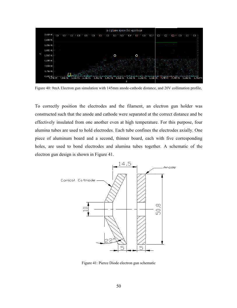
Figure
To c
const
effect
alumi
piece
holes
electr
e 40: 9mA Elec
correctly po
tructed such
tively insula
ina tubes are
e of aluminu
s, are used
ron gun desi
ctron gun simu
sition the e
that the ano
ated from on
e used to ho
um board a
to bond ele
ign is shown
Figu
ulation with 145
electrodes a
ode and catho
ne another e
ld electrode
and a second
ectrodes and
n in Figure 4
ure 41: Pierce D
50
5mm anode-ca
and the fila
ode were sep
even at high
s. Each tube
d, thinner b
d alumina t
1.
Diode electron
athode distance
ament, an e
parated at th
h temperatur
e confines th
board, each
tubes togeth
gun schematic
e, and 20V coll
electron gun
he correct di
re. For this p
he electrodes
with five c
her. A sche
c
limation profile
n holder wa
stance and b
purpose, fou
s axially. On
correspondin
ematic of th
e,
as
be
ur
ne
ng
he

51
To position the filament, an alumina tube with an inner radius equal to the radius of the
cathode hole was coaxially mounted next to the outer conical surface of the cathode. A
thinner alumina tube with the same outer radius as the cathode channel was inserted in to
the former tube. Two symmetric holes were drilled in the inner tube allowing the filament
to run across the gap inside the thinner tube, an insulation jacket tube made of alumina is
used to keep two ends of the filament away from each other.
In front of the holder, two copper wires were wrapped around the tubes to improve the
structural integrity of the electron gun assembly In order to apply voltage to electrodes,
two stainless steel wires were separately spot welded onto the conical cathode and the
plate anode. Because of the open structure of the holder, it was a simple process to
connect the leads from outside the device. Figure 42 shows the schematic for the electron
gun holder assembly.
Figure 42: Pierce-diode electron gun holding apparatus
The entire electron gun apparatus is about 0.1m in length and is mounted on the axial
center of the chamber at the end of the solenoid coil array at the vacuum chamber
midpoint. Table 11 shows theoretical parameters for varying anode-cathode distance for a
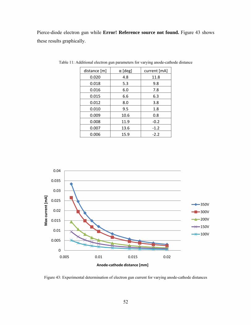
52
Pierce-diode electron gun while Error! Reference source not found. Figure 43 shows
these results graphically.
Table 11: Additional electron gun parameters for varying anode-cathode distance
distance [m] α [deg] current [mA]0.020 4.8 11.80.018 5.3 9.80.016 6.0 7.80.015 6.6 6.30.012 8.0 3.80.010 9.5 1.80.009 10.6 0.80.008 11.9 ‐0.20.007 13.6 ‐1.20.006 15.9 ‐2.2
Figure 43: Experimental determination of electron gun current for varying anode-cathode distances
0
0.005
0.01
0.015
0.02
0.025
0.03
0.035
0.04
0.005 0.01 0.015 0.02
Max current [m
A]
Anode‐cathode distance [mm]
350V
300V
200V
150V
100V
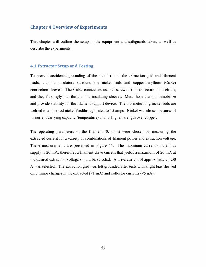
53
Chapter 4 Overview of Experiments This chapter will outline the setup of the equipment and safeguards taken, as well as
describe the experiments.
4.1 Extractor Setup and Testing To prevent accidental grounding of the nickel rod to the extraction grid and filament
leads, alumina insulators surround the nickel rods and copper-beryllium (CuBe)
connection sleeves. The CuBe connectors use set screws to make secure connections,
and they fit snugly into the alumina insulating sleeves. Metal hose clamps immobilize
and provide stability for the filament support device. The 0.5-meter long nickel rods are
welded to a four-rod nickel feedthrough rated to 15 amps. Nickel was chosen because of
its current carrying capacity (temperature) and its higher strength over copper.
The operating parameters of the filament (0.1-mm) were chosen by measuring the
extracted current for a variety of combinations of filament power and extraction voltage.
These measurements are presented in Figure 44. The maximum current of the bias
supply is 20 mA; therefore, a filament drive current that yields a maximum of 20 mA at
the desired extraction voltage should be selected. A drive current of approximately 1.30
A was selected. The extraction grid was left grounded after tests with slight bias showed
only minor changes in the extracted (<1 mA) and collector currents (<5 µA).

54
Figure 44: Biasing parameterization for 0.1 mm spherical filament
The parameters used to characterize the filament were initially extracted current as a
function of bias voltage and filament drive current. After characterizing the filament, the
actual extraction current detected at the collector plates (a distance of 0.5 meters from the
filament) was measured for a range of pressures. The pressure was controlled by varying
the amount of Argon gas leaking into the system through the venting system valve.
The rise in collector plate current shown in Figure 44 may also indicate an electron-beam
assisted discharge causes some of the current observed. The largest change in collector
current occurs above 1×10⁻⁶ Torr; therefore, the chamber should be kept below this
pressure while operating.
0
5
10
15
20
25
0 100 200 300 400 500 600
DC Extractor Cu
rren
t [mA]
Voltage [V]
1.30A
1.31A
1.32A
1.33A
1.34A
1.35A
1.36A
1.30A
1.31A
1.32A
1.33A
1.34A
1.35A
1.36A
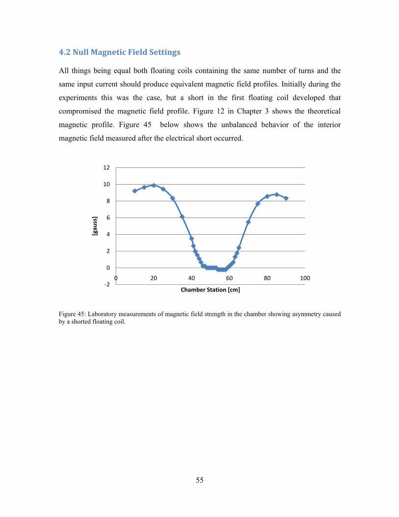
55
4.2 Null Magnetic Field Settings All things being equal both floating coils containing the same number of turns and the
same input current should produce equivalent magnetic field profiles. Initially during the
experiments this was the case, but a short in the first floating coil developed that
compromised the magnetic field profile. Figure 12 in Chapter 3 shows the theoretical
magnetic profile. Figure 45 below shows the unbalanced behavior of the interior
magnetic field measured after the electrical short occurred.
Figure 45: Laboratory measurements of magnetic field strength in the chamber showing asymmetry caused by a shorted floating coil.
‐2
0
2
4
6
8
10
12
0 20 40 60 80 100
[gau
ss]
Chamber Station [cm]
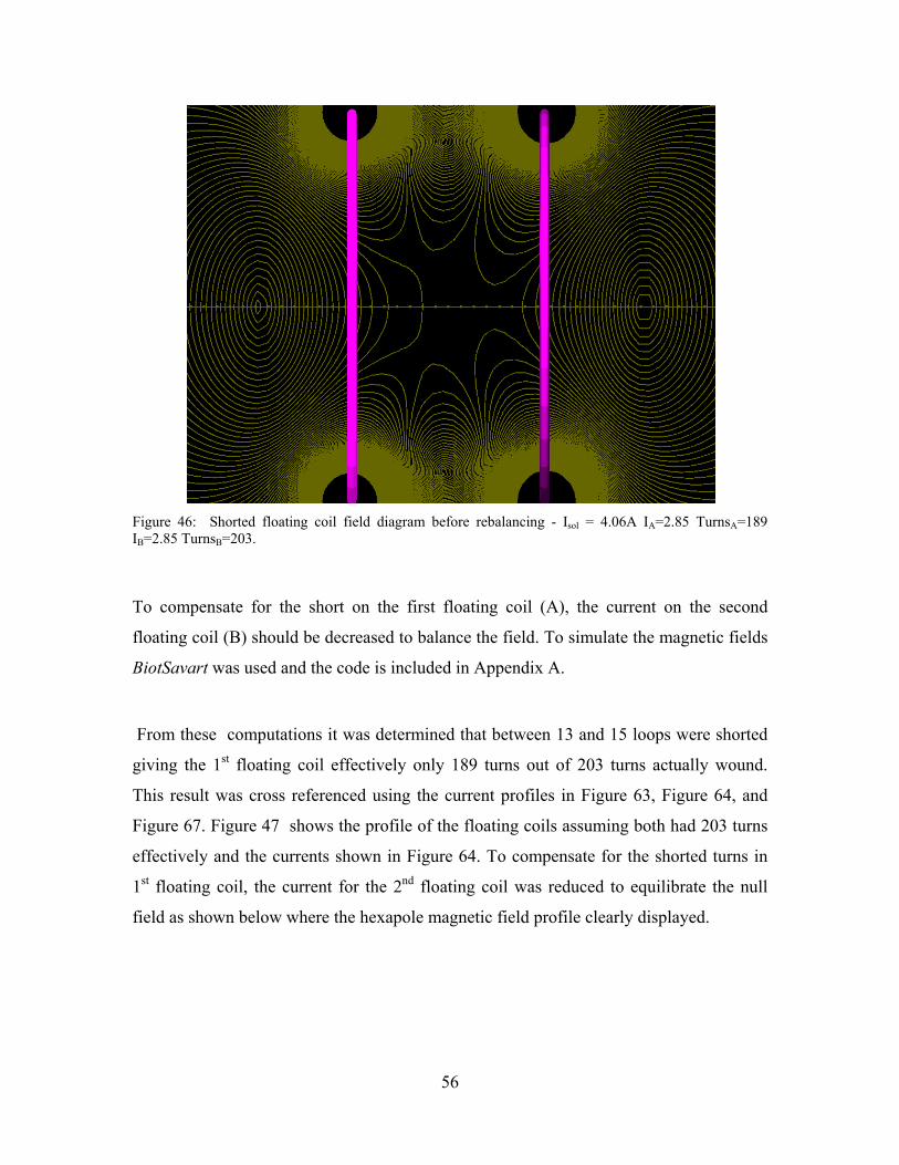
56
Figure 46: Shorted floating coil field diagram before rebalancing - Isol = 4.06A IA=2.85 TurnsA=189 IB=2.85 TurnsB=203.
To compensate for the short on the first floating coil (A), the current on the second
floating coil (B) should be decreased to balance the field. To simulate the magnetic fields
BiotSavart was used and the code is included in Appendix A.
From these computations it was determined that between 13 and 15 loops were shorted
giving the 1st floating coil effectively only 189 turns out of 203 turns actually wound.
This result was cross referenced using the current profiles in Figure 63, Figure 64, and
Figure 67. Figure 47 shows the profile of the floating coils assuming both had 203 turns
effectively and the currents shown in Figure 64. To compensate for the shorted turns in
1st floating coil, the current for the 2nd floating coil was reduced to equilibrate the null
field as shown below where the hexapole magnetic field profile clearly displayed.

57
Figure 47: Equilibration by reducing the current of the 2nd floating coil (B) – IA=2.85A & 189 Turns,
IB=2.65A & 203 Turns.
The correct rebalancing would have been to raise the current of the 1st floating coil (A) to
2.00A instead of lowering the 2nd floating coil (B) down to 1.66A. As a second check the
proper balancing at 20V on the solenoidal coils is shown in Table 12.
Table 12: Coil currents for 20V Solenoidal profile
1st floating coil (A) 2nd floating coil (B) Solenoidal Coil
Initial Current 2.85 Amperes 2.85 Amperes 4.06 Amperes
Turns ~189 effective turns 203 effective turns X
Experiment Current 2.85 Amperes 2.65 Amperes 4.06 Amperes
Figure 48 shows the null magnetic profile of the chamber before the current on the right
floating coil was adjusted for the 15 shorted coil turns (left) and the null profile after
rebalancing the coil system.
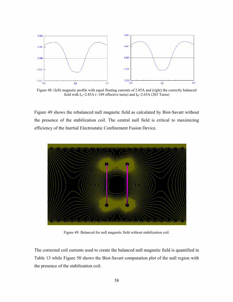
58
Figure 48: (left) magnetic profile with equal floating currents of 2.85A and (right) the correctly balanced
field with IA=2.85A (~189 effective turns) and IB=2.65A (203 Turns)
Figure 49 shows the rebalanced null magnetic field as calculated by Biot-Savart without
the presence of the stabilization coil. The central null field is critical to maximizing
efficiency of the Inertial Electrostatic Confinement Fusion Device.
Figure 49: Balanced for null magnetic field without stabilization coil.
The corrected coil currents used to create the balanced null magnetic field is quantified in
Table 13 while Figure 50 shows the Biot-Savart computation plot of the null region with
the presence of the stabilization coil.

59
Table 13: Coil Settings for Experiment Null Magnetic Field
Voltage [V] Current [A]
1st Floating Coil 6.2 -1.71
2nd Floating Coil 6.2 -1.59
Solenoidal Coil 11.7 3.71
Figure 50: Null magnetic field profile with stabilization coil – IA=-1.71A, IB=-1.59A, Istab=1.00A, Isol=4.35A
In addition to measuring filament and collector currents as a function of (controlled)
pressure, the (uncontrolled) rise in chamber pressure as a function of bias voltage and
extracted current was also measured. Figure 51 below details the increase of pressure that
coincides with the increase of bias voltage and extracted current. At 300 V, the chamber
pressure approaches 1×10⁻⁶ Torr, corresponding to the maximum desirable pressure.
Above this level ionizations from background gases effectively reduce electron transport
efficiency reducing collimation efficiency. However, electron bombardment cleans the
chamber, and the increase in pressure with bias voltage and extracted current decreases
with time as the chamber is cleaned. The data presented in Figure 51 was collected with
a very clean chamber (the maximum chamber pressure with no gas flow was
approximately 3-4×10⁻⁷ Torr at -300-V bias and 18 mA extracted current). In general,

60
measurements were not carried out until the chamber was clean enough that the 1×10⁻⁶
Torr pressure is never reached while operating the filament and extraction grid.
Figure 51: Dependence of Pressure on Filament Voltage
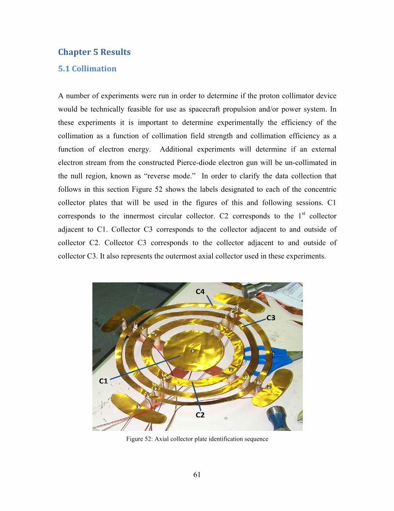
Chap
5.1 C A nu
woul
these
collim
funct
electr
the n
follow
collec
corre
adjac
collec
collec
pter 5 Re
Collimatio
umber of exp
d be technic
e experimen
mation as a
tion of elec
ron stream f
null region, k
ws in this se
ctor plates
esponds to t
cent to C1.
ctor C2. Co
ctor C3. It al
esults
on
periments we
cally feasibl
nts it is imp
function of
ctron energy
from the con
known as “
ection Figur
that will be
the innermo
Collector C
ollector C3
lso represent
Figure 5
ere run in or
le for use as
portant to d
f collimation
y. Addition
nstructed Pie
reverse mod
re 52 shows
e used in t
ost circular
C3 correspon
correspond
ts the outerm
52: Axial collec
61
rder to deter
s spacecraft
determine ex
n field stren
nal experim
erce-diode e
de.” In ord
s the labels d
the figures
collector. C
nds to the c
ds to the co
most axial co
ctor plate ident
rmine if the
propulsion
xperimentall
ngth and co
ments will d
electron gun
der to clarify
designated t
of this and
C2 correspo
collector adj
ollector adja
ollector used
tification seque
proton colli
and/or pow
ly the effic
llimation ef
determine if
will be un-
y the data c
to each of th
d following
onds to the
jacent to an
acent to an
d in these exp
ence
imator devic
er system. I
ciency of th
fficiency as
f an externa
-collimated i
ollection tha
he concentri
sessions. C
1st collecto
nd outside o
nd outside o
periments.
ce
In
he
a
al
in
at
ic
C1
or
of
of

62
After all collimator components where assembled, the collimator was operated with its
predicted operating parameters. The figure below shows the current extracted from the
filament as a function of the extraction voltage (DC bias voltage). This test serves as a
baseline for measuring collimation efficiency, as the electrons measured here are only
those emitted isotropically (no magnetic fields present).
Figure 53 shows the current of 300eV electrons measured in microamps at the concentric
collector plates in the absence of the collimating magnetic field for varying levels of
current extracted from the tungsten filament. The chart shows an increasing amount of
current collected at the axial plates as the level of extracted current increases. Deviation
from the expected linear increase can be attributed to varying pressure gradients. Figure
54 shows the same data as Figure 53 but as a function of electron energy.
Figure 53: Axial collector current without magnetic confinement as a function of extraction current
0
50
100
150
200
250
300
350
400
450
500
0 5 10 15 20
Collected
Current [µ
A]
Extraction Current [mA]
C1
C2
C3
C4
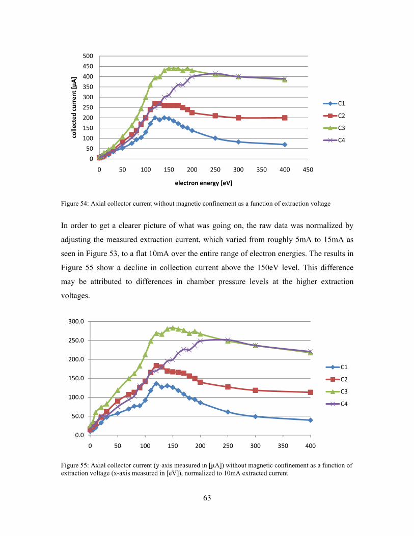
63
Figure 54: Axial collector current without magnetic confinement as a function of extraction voltage
In order to get a clearer picture of what was going on, the raw data was normalized by
adjusting the measured extraction current, which varied from roughly 5mA to 15mA as
seen in Figure 53, to a flat 10mA over the entire range of electron energies. The results in
Figure 55 show a decline in collection current above the 150eV level. This difference
may be attributed to differences in chamber pressure levels at the higher extraction
voltages.
Figure 55: Axial collector current (y-axis measured in [μA]) without magnetic confinement as a function of extraction voltage (x-axis measured in [eV]), normalized to 10mA extracted current
0
50
100
150
200
250
300
350
400
450
500
0 50 100 150 200 250 300 350 400 450
collected
current [μ
A]
electron energy [eV]
C1
C2
C3
C4
0.0
50.0
100.0
150.0
200.0
250.0
300.0
0 50 100 150 200 250 300 350 400
C1
C2
C3
C4

64
In these experiments there are three main variables that affect produce the unexpected
variations observed. The first is non-uniform variance in chamber pressure from a
number of contributions namely, cleanliness of the chamber off-gassing due to improper
use of non-vacuum rated adhesive during construction of the magnetic coils internal to
the vacuum chamber. This plays a role mainly in cases when moderate to excessive
current is applied to coils. Another contribution comes from variance in extracted current
versus extraction voltage. Every attempt was made to adjust these maintain these
parameters in a tight range, but were not always successful.
All internal coil currents were set to 1.1 amps, and the outer coil (solenoid) current was
set to 1.47 amps for these preliminary tests. As is evidenced there is a good amount of
collimation for our preliminary tests. The data above 200 V of bias may be false because
coil heating eventually lead to rapid off-gassing and a corresponding rapid rise in
pressure. The lower bias-voltage data is reliable because the off-gassing threshold of the
coils had not yet been reached.
Figure 56, which shows the effects of collimation at the 1.1A internal coil current level
and 1.45A solenoid coil level, can be directly compared to Figure 53. It can be easily
seen that more than five times as much current is present at the collector plates, clear
evidence of collimation.
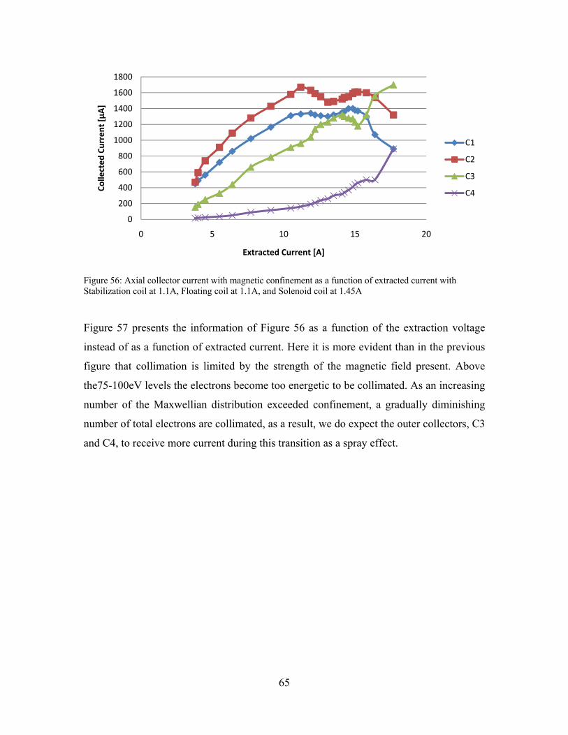
65
Figure 56: Axial collector current with magnetic confinement as a function of extracted current with Stabilization coil at 1.1A, Floating coil at 1.1A, and Solenoid coil at 1.45A
Figure 57 presents the information of Figure 56 as a function of the extraction voltage
instead of as a function of extracted current. Here it is more evident than in the previous
figure that collimation is limited by the strength of the magnetic field present. Above
the75-100eV levels the electrons become too energetic to be collimated. As an increasing
number of the Maxwellian distribution exceeded confinement, a gradually diminishing
number of total electrons are collimated, as a result, we do expect the outer collectors, C3
and C4, to receive more current during this transition as a spray effect.
0
200
400
600
800
1000
1200
1400
1600
1800
0 5 10 15 20
Collected
Current [µ
A]
Extracted Current [A]
C1
C2
C3
C4

66
Figure 57: Axial collector current with magnetic confinement as a function of extraction voltage [V] with Stabilization coil at 1.1A, Floating coil at 1.1A, and Solenoid coil at 1.45A
Figure 58 shows excellent linearization of collected current versus extracted current for
300eV electrons at a much higher magnetic field setting. Collimation is effective.
Figure 58: Axial collector plate current with magnetic confinement as a function of extraction current with
Floating coils both at 1.6A and Solenoid coil at 2.25A for 300 eV electrons
0
200
400
600
800
1000
1200
1400
1600
1800
0 50 100 150 200 250 300 350 400 450
Collected
Current [µ
A]
Extraction Voltage [V]
C1
C2
C3
C4
0
200
400
600
800
1000
1200
1400
1600
0 2 4 6 8 10 12 14
Collector Currents [µA]
Extraction Current [mA]

67
The collimator efficiency is estimated by summing the collector plate currents and
dividing the total by the current emitted by the filament. This is only an estimate because
it does not account for electrons lost to the extraction grid and electrons that struck the
Teflon between the collector plates. Because the collimator magnetic field is symmetric
along the z-axis, the highest possible efficiency for a single set of collector plates is 50%
because half of the extracted electrons travel away from the collector plates.
Figure 59 is the calculated collimation efficiency for one side of the collimator. As
expected when the energy of the electrons do not overpower the magnetic field strength
the collimation efficiency is approximately constant after the initial low current
fluctuations. This is expected behavior and demonstrates the success of the undertaking.
Figure 59: Collimation efficiency for the parameters corresponding to Figure 58
The efficiency of collimation depends on the energy of the electrons emitted from the
source-extractor assembly. Figure 85, in section 6.1 Collimation Efficiency, shows the
estimated collimator efficiency as a function of extraction voltage (electron source
energy).
0%
2%
4%
6%
8%
10%
12%
14%
16%
18%
20%
0 2 4 6 8 10 12
Collimation Efficiency
Extraction Current [mA]
collimation

68
5.2 Scattering – Reverse Mode Configuration The OOPIC simulation of Figure 60 shows that most of the electrons lost will be
channeled through the mid-point of the experiment focused on the positions of radial
collectors four and five while the remainder is collimated along the z-axis as designed
for. If neighboring collimators were attached on both sides, the equivalent collimated
particles entering from the neighbors could be anti-collimated in the central null-region.
To test this expected behavior an external electron source would be necessarily inserted
strategically inside the chamber in order to simulate the neighbors.
Figure 60: z-r phase space for 200 eV electrons after 100ns with stabilization coil active
To determine the operation of the reverse-mode configuration, scattering or anti-
collimation, an electron gun was built and installed at the end of the chamber where the
axial collectors were initially located. The axial collectors, near the end of the chamber
on the z-axis, were then moved to the other end of the chamber and the radial collectors
were installed around the floating coil configuration. The electron gun was a Pierce
diode configuration to minimize spread in the electron beam. The configuration is shown
in Figure 61. The radial collectors are numbered from left to right from one to eight. All
graphical data is pictured with the same orientation, i.e. radial collector 8 is always
closest to the electron gun and radial collector one is always closest to the axial collectors
for clarity in data presentation.

Figu
Figur
radia
Phase
for th
•
•
•
From
meter
right
partic
collec
expec
preve
impro
field
The p
coils
have
ure 61: Cross-saxial collector
re 62, Figure
l collector p
e I NASA S
hree main sce
Electron g
Electron g
Electron
stabilizati
m the first fo
r (hereafter
of the float
cles from on
ctor one, the
cted from an
ented accura
oved experim
configuratio
peaks near c
in between
a tendency
ectional diagrars surrounding
e 63, Figure
plate current
SBIR project
enarios at ea
gun only wit
gun with onl
gun with
ion, and floa
our figures c
AT/m) case
ting coils.
nly one side.
e distribution
n isotropic
ate assessme
ment would
on.
collectors th
collectors 2
to cross the
am of the chamthe floating co
64, Figure
readings for
t report27. T
ach power le
th no collima
ly the soleno
full collim
ating coils)
correspondin
es we see th
This is an
Had a seco
n would hav
source in th
ent of that h
d be necessa
ree and seve
2 & 3 and be
e magnetic fi
69
mber with radiaoils and the Pier
65, Figure 6
r the magnet
They show th
evel:
ating magne
oid magnetic
mating mag
ng to the 25
hat the curre
expected re
ond electron
e been symm
he center of
hypothesis i
ary to furthe
en are evide
etween 6 &
field line sep
al current collecrce-diode elect
66, and Figu
tic field setti
he measured
etic field
c field
gnetic field
, 50, 100, a
nts are sligh
sult as the
gun been uti
metric on bo
the null reg
n this stage
er verify the
enced by the
7. Here a sm
paratrix betw
ctors on the fartron gun on the
ure 67 show
ings determi
d collector c
d coils on
and 200 Am
htly off-cent
electron gun
ilized on the
oth sides, jus
gion. Spati
e of the exp
e scattering
e presence o
mall number
ween the floa
r left, the eighte far right.
the axial an
ined from th
current result
(solenoida
mpere-turn pe
ter and to th
n is injectin
e left of radia
t as would b
al limitation
eriment. A
effect of th
of the floatin
r of electron
ating coil an
t
nd
he
ts
al,
er
he
ng
al
be
ns
An
he
ng
ns
nd

70
the null region at the center. Some electrons become trapped around the closed field lines
of the floating coil much like in the presence of the closed field lines associated with a
magnetic dipole coil.
Figure 62: Axial and collector currents [µA] for 25 AT/m solenoidal coil field strength
Figure 63: Axial and collector currents [µA] for 50 AT/m solenoidal coil field strength
0
10
20
30
40
50
60
70
80
90
100
A1 A2 A3 A4 R1 R2 R3 R4 R5 R6 R7 R8
electron gun only EG and solenoidal coils EG, SC, and floating coils
0
10
20
30
40
50
60
70
80
90
100
A1 A2 A3 A4 R1 R2 R3 R4 R5 R6 R7 R8
electron gun only EG & solenoidal coils EG, SC, and floating coils

71
Figure 64: Axial and collector currents [µA] for 100 AT/m solenoid coil field strength
Figure 65: Axial and collector currents [µA] for 200 AT/m solenoidal coil field strength
Of further note is that up until 350 AT/m case, the magnetic field strengths are too weak
to effectively collimate the electrons. Figure 66 and Figure 67 are describing a
transitional state of the device where a portion of the electron beam is being deflected
into and eventually around the floating coil region which results in the fluctuation of
0
20
40
60
80
100
120
A1 A2 A3 A4 R1 R2 R3 R4 R5 R6 R7 R8
electron gun only EG & Solenoidal Coils EG, SC, & Floating Coils
0
20
40
60
80
100
120
140
A1 A2 A3 A4 R1 R2 R3 R4 R5 R6 R7 R8
Electron Gun Only EG & Solenoidal Coils EG, SC, & Floating Coils

72
currents measured by the radial collectors and finally some appreciable collimated
current measured on the first axial collector (A1 which is equivalent to C1 in previous
sections) as seen in Figure 67
Figure 66: Axial and collector currents [µA] for 350 AT/m solenoidal coil field strength
Figure 67: Axial and collector currents [µA] for 500 AT/m solenoidal coil field strength
0
50
100
150
200
250
300
350
400
A1 A2 A3 A4 R1 R2 R3 R4 R5 R6 R7 R8
Electron Gun Only EG & Solenoidal Coils EG, SC, & Floating Coils
0
50
100
150
200
250
300
350
A1 A2 A3 A4 R1 R2 R3 R4 R5 R6 R7 R8
Electron Gun Only EG & Solenoidal Coils EG, SC, & Floating Coils

Figur
gun a
streng
begin
occur
Figur
anti-c
streng
those
of th
collim
re 75 details
anti-collima
gth cases u
nning of the
r in earnest.
Figure 68:
re 69 is a sum
collimation/s
gth cases un
e detailed in
he transition
mation is sta
0
50
100
150
200
250
A1
a summary
tion/scatterin
under consid
transitional
: 3d surface rep
mmary of th
scattering e
nder conside
Figure 68. N
nal regime w
arting to occu
A2
of the axial
ng experime
deration. No
regime wher
presentation of
he radial coll
experiments
eration. Thes
Note that the
where the e
ur.
1 AT/
A3A4
73
collector pl
ents underta
ote that the
re collimatio
f axial collector
ector plate c
undertaken
se are in par
e 350 AT/m
electron gun
/m
50 AT/m
2
4
ate currents
aken for the
e 350 AT/m
on of the ele
r plate current
currents mea
n for the
rallel and of
field level ag
n beam is
200 AT/m
500 AT/
9
measured fo
e varying m
m field leve
ctron gun be
measurements
asured for all
varying ma
the same ex
gain marks t
perturbed s
/m
994 AT/m
or all electro
magnetic fiel
el marks th
eam begins t
s [µA]
l electron gu
agnetic fiel
xperiments a
the beginnin
signaling tha
200‐25
150‐20
100‐15
50‐100
0‐50
on
ld
he
to
un
ld
as
ng
at
0
0
0

Figure
Figur
readin
stabil
curre
once
the m
each
culmi
the m
10
15
20
25
30
e 69: 3D surfac
re 70, Figur
ngs for five
lization coil
ent collimate
the electron
magnetic fiel
profile with
inating in th
magnetic field
0
50
00
50
00
50
0
R1 R2
ce representatio
re 71, Figur
e different m
for the elect
ed increases
ns are more e
ld and escap
h an increasin
he much mor
d is strong e
R3 R4
on of radial col
re 72, Figur
magnetic fie
tron gun sca
as the the st
energetic tha
pe to the cha
ng shift of th
re linear pro
nough to con
4 R5
74
llector plate cu
re 73, and
eld strength
attering expe
trength of th
an 100 eV, th
amber walls.
he energetic
ogression of
nfine even 3
R6 R7
urrent measurem
Figure 74 d
levels with
eriments. As
e magnetic f
he particles a
The same
confinemen
the 20 Volt
300 eV electr
0 AT/m
10
R8
ments [µA]
detail the co
hout the pre
we expect t
field increas
are no longe
scenario is
nt peak furthe
t case in Fig
rons.
m
00 AT/m
994 AT/m
ollector plat
esence of th
the amount o
ses. Howeve
er confined b
played out i
er to the righ
gure 74 wher
250‐300
200‐250
150‐200
100‐150
50‐100
0‐50
te
he
of
er,
by
in
ht
re
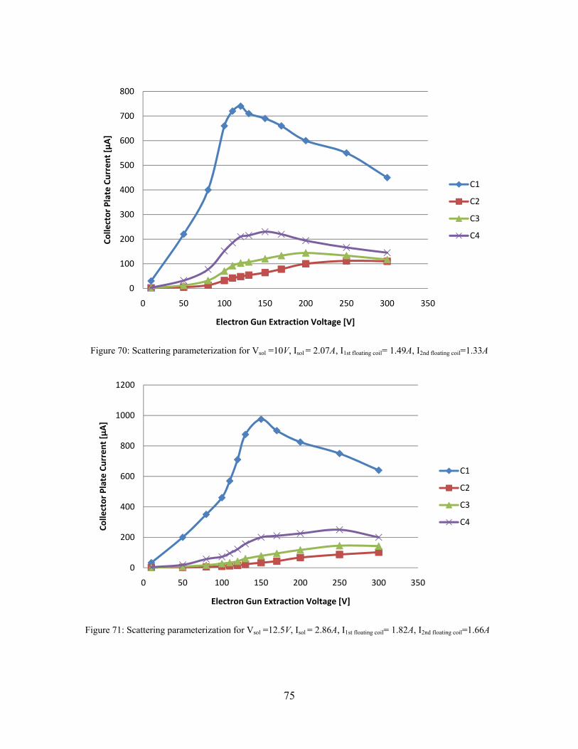
75
Figure 70: Scattering parameterization for Vsol =10V, Isol = 2.07A, I1st floating coil= 1.49A, I2nd floating coil=1.33A
Figure 71: Scattering parameterization for Vsol =12.5V, Isol = 2.86A, I1st floating coil= 1.82A, I2nd floating coil=1.66A
0
100
200
300
400
500
600
700
800
0 50 100 150 200 250 300 350
Collector Plate Current [μ
A]
Electron Gun Extraction Voltage [V]
C1
C2
C3
C4
0
200
400
600
800
1000
1200
0 50 100 150 200 250 300 350
Collector Plate Current [μ
A]
Electron Gun Extraction Voltage [V]
C1
C2
C3
C4

76
Figure 72: Scattering parameterization for Vsol =15V, Isol = 3.06A, I1st floating coil= 2.17A, I2nd floating coil=1.99A
Figure 73: Scattering parameterization for Vsol =17.5V, Isol = 3.56A, I1st floating coil= 2.51A, I2nd floating coil=2.32A
0
200
400
600
800
1000
1200
1400
0 50 100 150 200 250 300 350
Collector Plate Current [μ
A]
Electron Gun Extraction Voltage [V]
C1
C2
C3
C4
0
200
400
600
800
1000
1200
1400
0 50 100 150 200 250 300 350
Collector Plate Current [μ
A]
Electron Gun Extraction Voltage [V]
C1
C2
C3
C4

77
Figure 74: Scattering Parameterization for Vsol =20V, Isol = 4.06A, I1st floating coil= 2.85A, I2nd floating coil=2.65A
The behavior we expect is an increasing current reading at the central collector (C1) as
the magnetic field strength profile increases from the 10V to the 20V case. We also
would expect a decreasing amount of collected current at each progressively outward
collector as the magnetic field profile increases reflecting that the electrons are being a
more tightly collimated toward the chamber centerline. From the OOPIC simulations a
channeling phenomenon was observed with noticeable voids in electron current between
3.1 and 7.4 cm from the chamber centerline which is illustrated below in Figure 75.
Figure 75: Current profile for collector plate region on the 22.5 volt solenoid voltage case
0
200
400
600
800
1000
1200
1400
1600
0 50 100 150 200 250 300 350
Collector Plate Current [μ
A]
Electron Gun Extraction Voltage [V]
C1
C2
C3
C4
0
0.000005
0.00001
0.000015
0.00002
0.000025
0.00003
0.000035
0.00004
0.13
100.12
600.12
100.11
600.11
100.10
600.10
100.09
600.09
100.08
600.08
100.07
600.07
100.06
600.06
100.05
600.05
100.04
600.04
100.03
600.03
100.02
600.02
100.01
600.01
100.00
600.00
10
collected
current [A
]
radial station location [m]

Figur
gun s
the in
exper
magn
indee
incre
previ
energ
on th
Figuresoleno
Figur
electr
behav
Curren
t [μA]
re 76, Figure
scattering ex
nnermost fir
rimental res
nitudes and
ed shows an
ased. Also i
ious section
getic to be co
e center coll
e 76: Center cooidal voltage st
re 77 and F
ron density
vior is consi
0
200
400
600
800
1000
1200
1400
Extr
e 77, Figure
xperiments o
rst and work
sults accurat
particle cha
increasing
important to
, it is obse
ollimated at
lector decrea
oncentric colletrength
Figure 78 be
is more co
stent through
raction Voltage
78, and Fig
on each of th
king outwar
tely reflect
anneling. Fig
level of col
o note is tha
rved that p
the 10V ma
ases.
ector plate (C1
elow show t
oncentrated t
hout the enti
e [V]
78
gure 79 show
he concentri
rd in accord
the expecte
gure 76, whi
limated curr
at similar to
ast the 150
agnetic field
) current profi
that as the
toward the
ire range of
10
w the curren
ic axial coll
dance with F
ed behavior
ich details t
rent as the m
o the collim
0eV level th
d strength pro
ile versus elect
magnetic fie
center colle
electron ene
012.5
15
t profiles for
ector plates
Figure 52. In
in terms o
the center co
magnetic fie
mation experi
he electrons
ofile and the
tron gun extrac
eld strength
ector of Fig
ergies under
17.520
r the electro
starting wit
n general th
f collimatio
ollector (C1
ld strength i
iments in th
become to
e total curren
ctor voltage an
h is increase
gure 69. Thi
study.
1200‐1400
1000‐1200
800‐1000
600‐800
400‐600
200‐400
0‐200
on
th
he
on
),
is
he
oo
nt
nd
ed
is

Figuresoleno
Figuresoleno
10
e 77: 2nd concoidal voltage st
e 78: 3rd concoidal voltage st
10
15
10
12.5
15
175
centric collectotrength
centric collectotrength
20
17.5
20
5010
or plate (C2) c
or plate (C3) c
Ext
10080
Extr
79
current profile
current profile
raction Voltag
13120
110
action Voltage
versus electro
versus electro
ge [V]
20170150
0
e [V]
on gun extract
on gun extract
0
20
40
60
80
1
1
0
20
40
60
80
10
12
14
1
30025000
tion voltage an
tion voltage an
0
0
0
0
00
120
Curren
t [μA
]
100‐120
80‐100
60‐80
40‐60
20‐40
0‐20
0
0
00
20
40
60
Curren
t [μA
]
140‐160
120‐140
100‐120
80‐100
60‐80
40‐60
20‐40
0‐20
nd
nd

Figuresoleno
5.3 C The n
striki
This
perpe
the c
This
electr
a para
Initia
The r
some
groun
10
e 79: 4th concoidal voltage st
Collimated
next set of
ing the axial
is importan
endicular com
ollimator as
could easily
ron source p
allel compon
ally, each co
results of th
e collector
nded (as opp
10
12.5
15
175
centric collectotrength
d Particle
experiments
collector pl
nt in order to
mponent of
s particles b
y be accom
potential and
nent greater
ollector plate
ese test show
plates. Th
posed to floa
17.5
20
5010
or plate (C4) c
Energy
s was used
lates from th
o determine
the magnetic
ecome trapp
mplished by
d measuring
than the floa
e current wa
w large and
he measurem
ating) except
10080
Ext
80
current profile
to determin
he 300 eV el
how much
c field which
ped in the n
allowing th
the current
ating potenti
as measured
d erratic fluc
ments were
t for the coll
1120
110
traction Voltag
versus electro
ne the energ
lectron sourc
of the elect
h ultimately
null region l
e collector
noting that o
ial will strike
d with the re
tuations in t
repeated w
lector plate b
2170
15030
ge [V]
on gun extract
gy level of
ce after bein
tron energy
reduces the
ike in a ma
plates to flo
only those e
e the collect
emaining pl
the currents
with all col
being measu
0
5
1
300250200
tion voltage an
the electron
ng collimated
is lost to th
efficiency o
agnetic bottle
oat up to th
electrons wit
tor plates.
lates floating
measured o
llector plate
ured, which i
0
50
100
150
200
250
Curren
t [μA
]
200‐250
150‐200
100‐150
50‐100
0‐50
nd
ns
d.
he
of
e.
he
th
g.
on
es
is
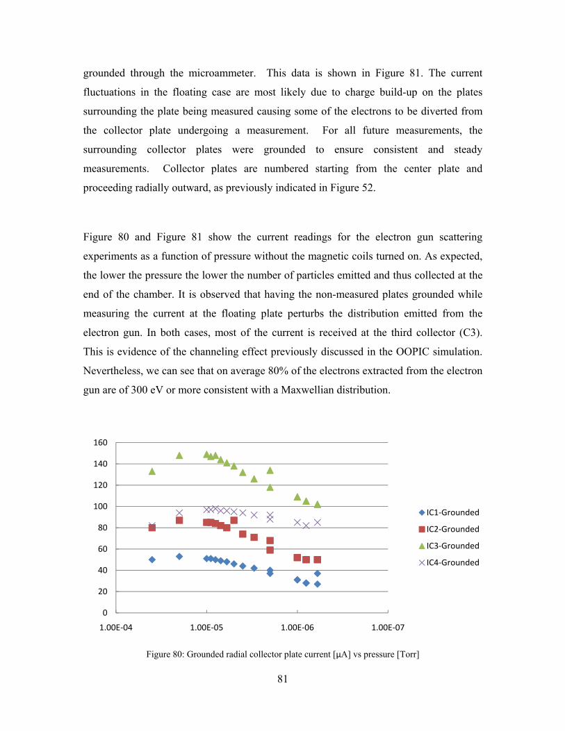
81
grounded through the microammeter. This data is shown in Figure 81. The current
fluctuations in the floating case are most likely due to charge build-up on the plates
surrounding the plate being measured causing some of the electrons to be diverted from
the collector plate undergoing a measurement. For all future measurements, the
surrounding collector plates were grounded to ensure consistent and steady
measurements. Collector plates are numbered starting from the center plate and
proceeding radially outward, as previously indicated in Figure 52.
Figure 80 and Figure 81 show the current readings for the electron gun scattering
experiments as a function of pressure without the magnetic coils turned on. As expected,
the lower the pressure the lower the number of particles emitted and thus collected at the
end of the chamber. It is observed that having the non-measured plates grounded while
measuring the current at the floating plate perturbs the distribution emitted from the
electron gun. In both cases, most of the current is received at the third collector (C3).
This is evidence of the channeling effect previously discussed in the OOPIC simulation.
Nevertheless, we can see that on average 80% of the electrons extracted from the electron
gun are of 300 eV or more consistent with a Maxwellian distribution.
Figure 80: Grounded radial collector plate current [μA] vs pressure [Torr]
0
20
40
60
80
100
120
140
160
1.00E‐071.00E‐061.00E‐051.00E‐04
IC1‐Grounded
IC2‐Grounded
IC3‐Grounded
IC4‐Grounded

82
Figure 81: 300 eV radial collector plate current [μA] vs pressure [Torr]
From this data it becomes apparent that a combination of factors including the
positioning of the electron gun and the anode-cathode difference were not closely
matched well enough to adequately simulate the additional particles that would enter
from a neighboring collimator.
The other conclusion that can be drawn from this data is the divergence from the
behavior observed in OOPIC simulations. Figure 60 shows that most of the escaping
electrons are channeled through the central region focused on the positions of radial
collectors four and five. One can deduce that there is no equivalent defocusing of
electrons entering the null region of the magnetic field from the electron gun.
0
20
40
60
80
100
120
140
160
1.00E‐071.00E‐061.00E‐051.00E‐04
IC1‐Floating
IC2‐Floating
IC3‐Floating
IC4‐Floating

83
Chapter 6 Interpretation
6.1 Collimation Efficiency The efficiency of collimation depends on the energy of the electrons emitted from the
source-extractor assembly. Figure 85 shows the estimated collimator efficiency as a
function of extraction voltage (electron source energy). The collimator efficiency is
estimated by summing the collector plate currents and dividing the total by the current
emitted by the filament. This is only an estimate because it does not account for
electrons lost to the extraction grid and electrons that passed between the gap between the
individual collector plates shows in Figure 52. As we have seen previously from both the
electron gun experiments and the OOPIC simulations, as shown in Figure 75, electron
channels form creating current voids, thus using a current average from the two adjacent
collectors may not be accurate beyond a first approximation. This averaged
approximation was compared with a measurement of the full collector region in OOPIC
simulations and was shows to have a maximum 11% margin of error in total current.
Depending on the magnetic field strength the averaging estimate can be higher or lower
than the actual current. To reiterate because of symmetry along the z-axis, the highest
possible efficiency for a single set of collector plates is 50%. Figure 82 demonstrates an
excellent level of collimation up to around 50 eV (horizontal axis) after which the
electrons are too energetic for the magnetic field strength for optimum collimation.

84
Figure 82: Collimation efficiency as a function of electron energy [eV] - Stabilization coil at 1.1A, Floating coil at 1.1A, Solenoid Coil at 1.45A as related to data from Figure 56 and Figure 57
Figure 83: Comparison of normalized collector currents against the total extracted current (I-ext) versus electron energy for the electron gun scattering experiments
0%
5%
10%
15%
20%
25%
30%
35%
40%
45%
0 100 200 300 400 500
effciency
electron energy [eV]
uncollimated
collimated
0
2000
4000
6000
8000
10000
12000
0 50 100 150 200 250 300 350
Curren
t [µA
]
Electron Energy (eV)
10.0V
12.5V
15.0V
17.5V
I‐ext

85
As we expect, Figure 84 shows that the collimation efficiency is not dependent on the
level of extraction current but primarily on the ratio of field strength to particle energies.
Figure 84: Extrapolated collimation efficiency versus extraction current for 300 eV electrons corresponding to data from Figure 58 and Figure 83 for Floating Coils at 1.6A and Solenoid coil at 2.25A
Figure 85 details the collimation efficiency for the electron gun experiments under 5
particular magnetic field profile settings. In most profiles there is a general trend shifting
the peak further to the right as would be expected, however pressure and extraction
current anomalies created distortions particularly in the 15V and 20V cases. Pressure
anomalies were primarily due to off-gassing of the internal coils.
0%
5%
10%
15%
20%
25%
30%
35%
0 2 4 6 8 10 12
extraction current [mA]
efficiency

86
Figure 85: Collimator Efficiency as a Function of Extraction Voltage and Solenoid Voltage for the electron gun scattering experiments
Off-gassing from coil heating was a major concern. As previously mentioned in section
3.3 Floating Coils, there was a construction flaw that used a non-vacuum rated adhesive
to bind initial windings of the floating and stabilization coil cores together. Thus, when
operating at power for an appreciable amount of time coil heating produces carbon
contamination in the vacuum chamber. To examine the effect of coil heating, data was
taken starting at high bias voltages (400V) and reducing the bias voltage as the
measurements progressed in an attempt to keep pressure as close to a constant as possible
before heating caused a rapid pressure rise.
The figure below shows pressure as a function of voltage during this test. Again, the
pressure rose rapidly after a certain coil operating time; in this case, the out-gassing
began near 150 V. A discontinuity in the collimated data exists because a data point was
sacrificed to complete the measurement set before pressure climbed too high.
0%
5%
10%
15%
20%
25%
30%
0 50 100 150 200 250 300 350
efficiency
extracted electron energy [eV]
10.0V
12.5V
15.0V
17.5V
20.0V

87
0 100 200 300 400
10-6
Pre
ssur
e [T
orr]
Extraction Voltage
no collimation w/ collimation
Figure 86 Coil heating effect on pressure as a function of electron energy in eV
In experiments, collimation has been observed for electron energy less than several
hundred eV. Higher energy electrons increase losses to the vacuum chamber wall and
results in decreasing collimation current as expected.

88
Chapter 7 Particle Simulation Nieto24 developed the preliminary particle trajectory calculations for the proton
collimator or as he referred to it, the Proton Diverter Converter, (PDC) in 2001. The first
part of those calculations dealt with single particle trajectories that would yield the
scaling relations and the device configuration, most notably the size and location of the
floating and stabilization coils. The magnetic field configuration was chosen to have a
null field at the center of the device where an inertial electrostatic confinement fusion
device would be located fueled by neutral beam injectors and charged to a grid potential
of -100 kV.
After the initial sizing parameters were determined, Nieto expanded the scope of the
project by developing a single-particle Monte Carlo code to better model the particles
traveling inside the collimator known as TOSPEMF (the Trajectory Of a Single Particle
on Electric and Magnetic Fields). At the time of that work, most existing codes were
designed with magnetic mirrors and Field Reverse Configuration devices in mind. The
hexapole generated null region of the collimator made these particle tracking codes
unusable because in the null field region the magnetic moment, Larmor Radius, and gyro-
frequency of the particles become either zero or infinite. The TOSPEMF code was
expanded to account for particle groups of up to 10,000 particles.
In order to gain further insight into device operation of the proton collimator, simulations
for this thesis were run specific to the electron collimator simulator that corresponds to
the body of this work. XOOPIC/OOPIC Pro is a 2D particle-cell-code (PIC) code with
electrostatic and electromagnetic field solvers with support for cylindrical geometries. It
is well capable of simulating physical systems including plasmas, beams of charged
particles, externally generated electric and magnetic fields, low-to moderate density
neutral gases, and a wide variety of boundary conditions. There are also subroutines for
Monte Carlo Collisions, user-defined diagnostics, and collisional cross-sections.
XOOPIC28 also includes the expanded capability to include fusion cross-sections,
reactions, and floating potential conductors29.

89
7.1 Numerical Considerations The two fundamental aspects of any XOOPIC/OOPIC simulation are the grid and control
blocks of the input file. The grid specifies the physical dimensions of the simulated
regions and the control specifies the time step and the electromagnetic field solver to use.
The ElectrostaticFlag was set to zero which corresponds to a full update of Maxwell’s
equations and the geometry chosen was cylindrical as the experiment was symmetrical
about the z-axis.
One of the most important considerations in selecting the grid and time-step for the
simulation is ensuring convergence of the hyperbolic partial differential equations used in
the PIC code. For example, if an electron is crossing a discrete grid, then the timestep
must be less than the time for the electron to travel to adjacent grid points. As a corollary,
when the grid point separation is reduced, the upper limit for the time step also decreases.
In essence, the numerical domain of dependence must include the analytical domain of
dependence in order to assure that the solver can access the information required to form
the solution. This is known as the Courant-Friedrichs-Lewy condition30 and for the
simulation under consideration is known as
r zu t u t Cr z
⋅ Δ ⋅ Δ+ ≤
Δ Δ
Where u is the velocity, Δt is the time step, Δr and Δz are the particle dimensions and C is
a constant dependent on the equations of motion and thus Maxwell’s equations. Another
constraint is the computational power of the machine running the simulation. A typical
1000x1000 grid area results in an array of 1 million cells. Above the 2 million particle
cell threshold is pushing the limits of most desktop computers thus the goal for
computational efficiency was to stay under the 2 million particle cell limit. As this
simulation models the actual size of the electron collimator simulator experiment, the
particle cell dimensions were chosen to be 0.5 mm squares resulting in a 2000 x 600 cell

90
array. With the typical velocity of a 300eV electron being on the order of 1x10⁷ m/s the
upper limit of the time step was determined to be on the order of 1x10-12 seconds.
Table 14: Particle cell parameters used in OOPIC/XOOPIC simulation
Particle cells Physical dimension [meters]z-axis chamber & sim limit 2000 1.00000 m
r-axis sim limit 600 0.30000 m r-axis chamber limit 495 0.24975 m
The particles under consideration are electrons simulating protons. As such the species
was named eprotons and defined with the mass and charge of the electron. The particles
utilized an electron-electron collisional model31.
The boundary conditions for the edge of the simulation were chosen to be perfect
conductors grounded to zero. While the electron gun anode and cathodes were modeled
as Equipotenials which are capable of time dependent variations.
7.2 Magnetic Coil Modeling The magnetic coils were modeled as current regions with each solenoid coil being one
contiguous current region. In the program the total current in the cross sectional region is
defined by the following relation:
where coilCurrent is the total current applied from the power supply, coilTurns is the
total number of turns for the coil under consideration (203 turns for the floating coil, 80
turns for the stabilization coil, and 24 turns for each solenoid coil), and coilRatio is the
ratio of the segment cross sectional area to the total cross sectional area. Figure 87 shows
the segments defined for the floating coil. For example, the center region denoted in red
represents 121 out of 177 total cross sectional units (11×11). Each green segment
represents 7 out of 177 total cross sectional units (1×7). Finally each black segment
represents 5 out of the 177 total cross sectional units (1×5).
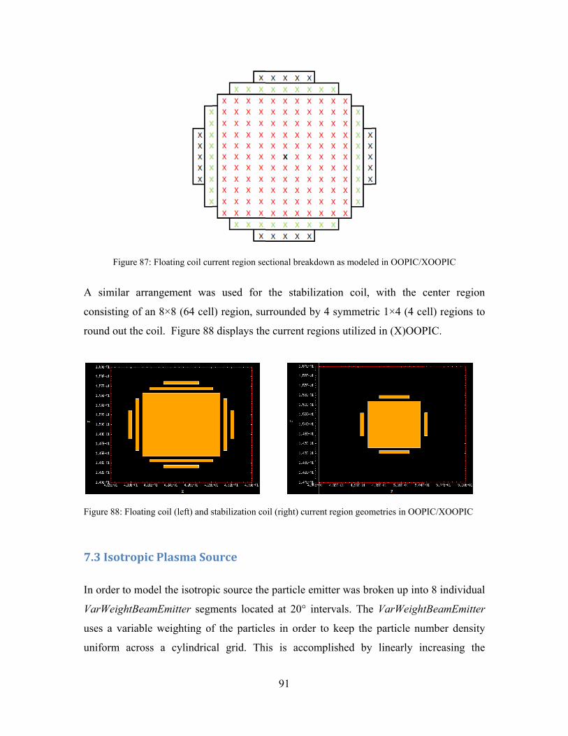
A sim
consi
round
Figure
7.3 I
In ord
VarW
uses
unifo
Figure 87: Fl
milar arrang
isting of an
d out the coi
e 88: Floating c
Isotropic P
der to model
WeightBeamE
a variable w
orm across
loating coil cur
gement was
8×8 (64 cell
l. Figure 88
coil (left) and s
Plasma So
l the isotrop
Emitter segm
weighting of
a cylindrica
rrent region se
s used for
l) region, su
8 displays the
stabilization co
urce
ic source the
ments locate
f the particl
al grid. Th
91
ctional breakd
the stabiliz
urrounded by
e current reg
oil (right) curre
e particle em
ed at 20° in
es in order
is is accom
own as modele
zation coil,
y 4 symmetr
gions utilized
ent region geom
mitter was br
ntervals. The
to keep the
mplished by
ed in OOPIC/X
with the c
ric 1×4 (4 ce
d in (X)OOP
metries in OOP
roken up into
e VarWeight
e particle nu
y linearly in
XOOPIC
center regio
ell) regions t
PIC.
PIC/XOOPIC
o 8 individua
tBeamEmitte
umber densit
ncreasing th
on
to
al
er
ty
he

92
weighting factor of the particles with the radius for cylindrical geometries31. Each
segment is two cells wide or 1.0 mm in diameter in order to more closely approximate the
wire width of the extraction grid. Each segment was placed at the location of the
extraction grid where the emitted electron velocity was maximized rather than placed at
the emitter radius and accelerated to full potential. One issue with this setup was a
relatively high number of particles were forced back onto the extraction grid due to space
charge limitations. The implications of this is detailed in
7.4 Cases Simulated. Each segment was divided into equivalent levels of extracted
current except those at the axis of symmetry which were allocated half the allotted
segment current. This segmented geometry is an acceptable approximation to an isotropic
source and models the experimental configuration well. Coordinates used are detailed in
Table 15 while Figure 89 shows a closeup of the emitter region under operation in
(X)OOPIC.
Table 15 Isotropic electron source segment positioning and kinetic energy definitions
Z-min Z-max R-min R-max VZ [eV] VR [eV]
0° 1050 1050 1 0 300 0
20° 1048 1048 15 14 282 103
40° 1041 1041 31 30 230 103
60° 1028 1029 45 45 150 260
80° 1011 1012 50 50 52 295
100° 988 989 50 50 -52 295
120° 971 972 45 45 -150 260
140° 959 959 30 31 -230 193
160° 952 954 14 15 -282 103
180° 950 950 0 1 -300 0
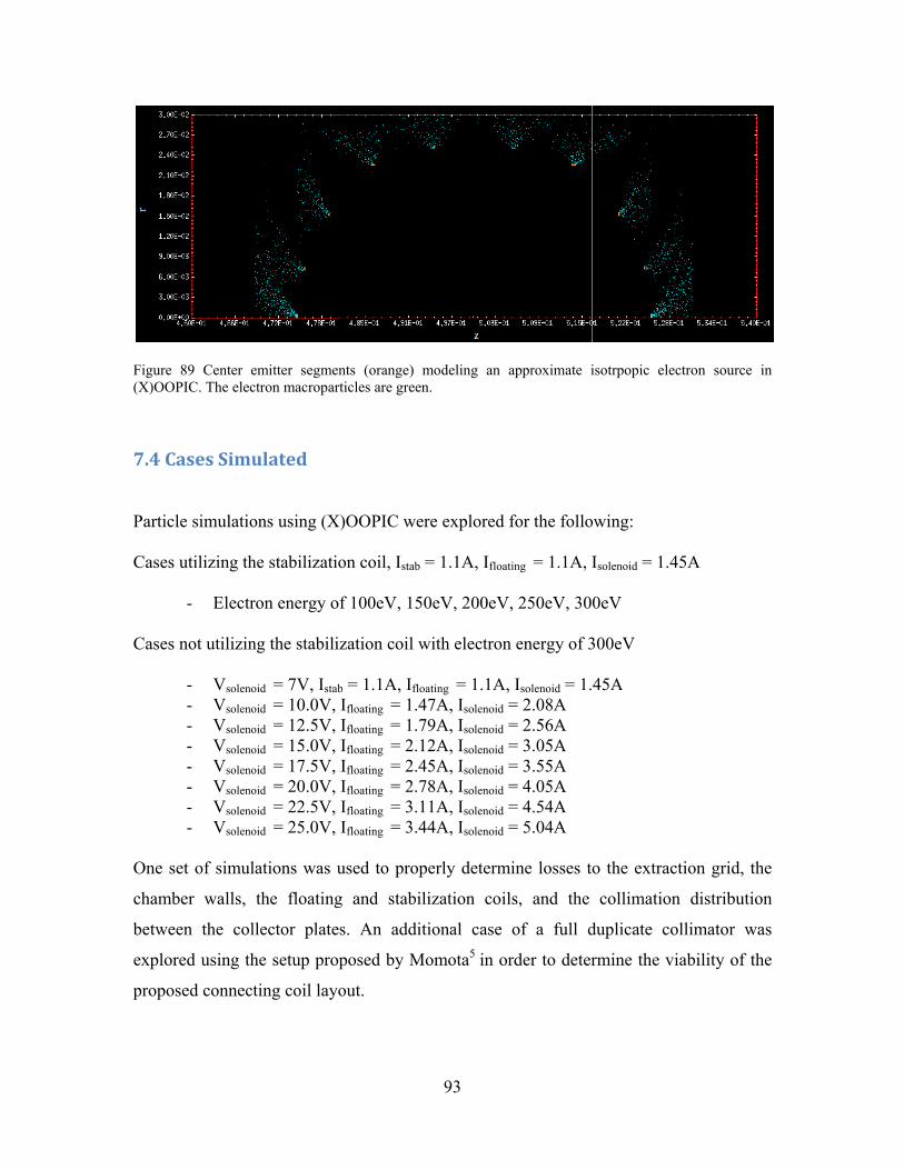
Figure(X)OO
7.4 C Partic Cases
Cases
One
cham
betwe
explo
propo
e 89 Center eOPIC. The elec
Cases Simu
cle simulatio
s utilizing th
- Electr
s not utilizin
- Vsoleno- Vsoleno- Vsoleno- Vsoleno- Vsoleno- Vsoleno- Vsoleno- Vsoleno
set of simul
mber walls,
een the col
ored using th
osed connect
emitter segmectron macropar
ulated
ons using (X
he stabilizati
ron energy o
ng the stabili
oid = 7V, Istab
oid = 10.0V, oid = 12.5V, oid = 15.0V, oid = 17.5V, oid = 20.0V, oid = 22.5V, oid = 25.0V,
lations was u
the floating
llector plate
he setup pro
ting coil lay
nts (orange) mrticles are green
X)OOPIC we
on coil, Istab
of 100eV, 15
ization coil w
b = 1.1A, IfloIfloating = 1.4Ifloating = 1.7Ifloating = 2.1Ifloating = 2.4Ifloating = 2.7Ifloating = 3.1Ifloating = 3.4
used to prop
g and stabil
es. An addit
posed by M
out.
93
modeling an n.
ere explored
= 1.1A, Ifloa
0eV, 200eV
with electron
oating = 1.1A,47A, Isolenoid79A, Isolenoid12A, Isolenoid45A, Isolenoid78A, Isolenoid11A, Isolenoid44A, Isolenoid
perly determ
lization coil
tional case
Momota5 in o
approximate i
for the follo
ating = 1.1A, I
V, 250eV, 30
n energy of 3
, Isolenoid = 1.= 2.08A = 2.56A = 3.05A = 3.55A = 4.05A = 4.54A = 5.04A
mine losses t
ls, and the
of a full d
rder to deter
isotrpopic elec
owing:
Isolenoid = 1.4
0eV
300eV
45A
o the extrac
collimation
duplicate co
rmine the vi
ctron source i
45A
ction grid, th
n distributio
ollimator wa
iability of th
in
he
on
as
he
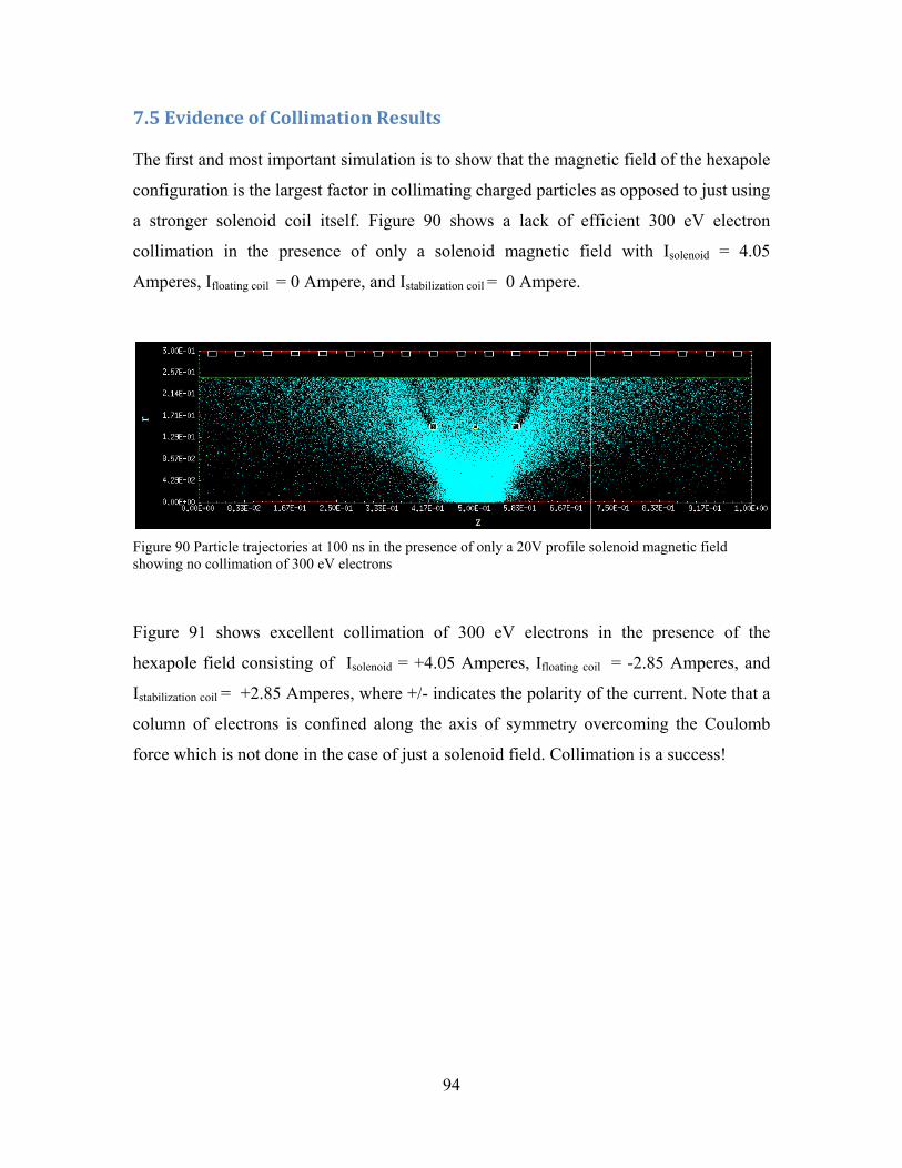
7.5 E The f
confi
a stro
collim
Amp
Figureshowin
Figur
hexap
Istabiliz
colum
force
Evidence o
first and mos
iguration is t
onger solen
mation in th
eres, Ifloating c
e 90 Particle trang no collimat
re 91 show
pole field co
zation coil = +2
mn of electr
which is no
of Collimat
st important
the largest fa
noid coil itse
he presence
coil = 0 Amp
ajectories at 10tion of 300 eV
ws excellent
onsisting of
2.85 Ampere
rons is confi
ot done in the
tion Resul
simulation i
actor in colli
elf. Figure
e of only a
pere, and Istab
00 ns in the preelectrons
collimation
Isolenoid = +
es, where +/
fined along t
e case of jus
94
lts
is to show th
mating char
90 shows a
a solenoid m
bilization coil =
esence of only
n of 300 eV
+4.05 Amper
/- indicates th
the axis of
t a solenoid
hat the magn
rged particles
a lack of ef
magnetic fi
0 Ampere.
a 20V profile s
V electrons
res, Ifloating co
he polarity o
symmetry o
field. Collim
netic field of
s as opposed
fficient 300
eld with Iso
solenoid magn
in the pre
oil = -2.85 A
of the curren
overcoming
mation is a su
f the hexapol
d to just usin
eV electro
olenoid = 4.0
netic field
sence of th
Amperes, an
nt. Note that
the Coulom
uccess!
le
ng
on
05
he
nd
a
mb
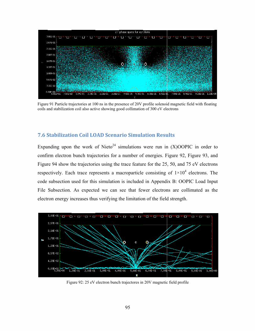
Figurecoils a
7.6 S Expa
confi
Figur
respe
code
File
electr
e 91 Particle traand stabilizatio
Stabilizati
anding upon
irm electron
re 94 show t
ectively. Eac
subsection u
Subsection.
ron energy in
Fig
ajectories at 10on coil also acti
on Coil LO
the work o
bunch traje
the trajectori
ch trace rep
used for this
As expecte
ncreases thu
gure 92: 25 eV
00 ns in the preive showing go
OAD Scena
of Nieto24 s
ectories for a
ies using the
resents a m
s simulation
ed we can
us verifying t
electron bunch
95
esence of 20V pood collimation
ario Simula
simulations
a number of
e trace featur
macroparticle
n is included
see that few
the limitation
h trajectores in
profile solenoin of 300 eV ele
ation Resu
were run in
f energies. F
re for the 25
e consisting
d in Appendi
wer electron
n of the field
n 20V magnetic
id magnetic fieectrons
ults
n (X)OOPIC
Figure 92, Fi
, 50, and 75
of 1×10⁴ e
ix B: OOPIC
ns are collim
d strength.
c field profile
eld with floatin
C in order t
igure 93, an
eV electron
lectrons. Th
C Load Inpu
mated as th
g
to
nd
ns
he
ut
he

7.7 S
One
stabil
1.1A,
the el
and 3
proxi
decre
cham
Fig
Fig
Stabilizati
of the cases
lization coil.
, Ifloating = 1
lectron macr
300 eV resp
imity to the
ease as wou
mber. While
ure 93: 50 eV
ure 94: 75 eV
on Coil Sc
s under stud
. Specifically
1.1A, Isolenoid
roparticle di
pectively. As
e floating co
uld be evide
the proxim
electron bunch
electron bunch
enario Sim
dy in this th
y the magne
d = 1.45A. F
istribution af
s the particle
oils should
enced by a
mity of the e
96
h trajectories in
h trajectories in
mulation R
hesis is the
etic profile c
Figure 95, Fi
fter 100 ns f
e energy lev
decrease, a
lower densi
electrons to
n 20V magnetic
n 20V magnetic
Results
level of col
characterized
igure 96, an
for energy le
vel increases
and the leve
ity of electr
the floating
c field profile
c field profile
llimation wi
d by Vsolenoid
nd Figure 97
evels of 100
s, we expect
el of collim
rons at the
g coils does
ith the activ
= 7V, Istab
7 below show
0 eV, 200 eV
t the electro
mation shoul
edges of th
s decrease,
ve
=
w
V,
on
ld
he
it
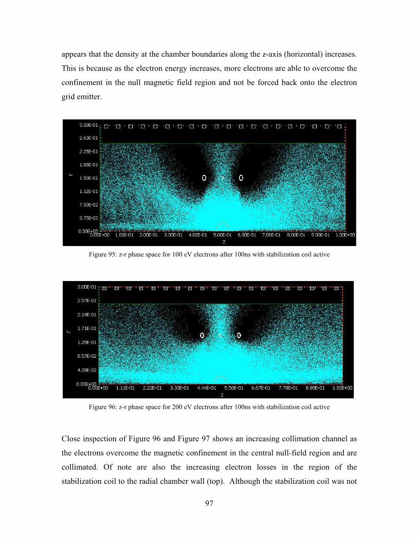
97
appears that the density at the chamber boundaries along the z-axis (horizontal) increases.
This is because as the electron energy increases, more electrons are able to overcome the
confinement in the null magnetic field region and not be forced back onto the electron
grid emitter.
Figure 95: z-r phase space for 100 eV electrons after 100ns with stabilization coil active
Figure 96: z-r phase space for 200 eV electrons after 100ns with stabilization coil active
Close inspection of Figure 96 and Figure 97 shows an increasing collimation channel as
the electrons overcome the magnetic confinement in the central null-field region and are
collimated. Of note are also the increasing electron losses in the region of the
stabilization coil to the radial chamber wall (top). Although the stabilization coil was not

98
modeled with a conductor, a user-defined diagnostic measured the electron current flow
through the stabilization coil region and subtracted off the wall losses.
Figure 97: z-r phase space for 300eV electrons after 100ns with stabilization coil active under the 20V magnetic field strength profile
Figure 99 shows the effect of a much stronger magnetic field profile on collimation when
compared to Figure 97. Also note that the 35V is still in a transient state but close enough
to steady-state to be a good representation of particle trajectories.
Figure 98: z-r phase space for collimation of 300 eV electrons after 60 ns under the 35V magnetic field strength profile
Figure 99 shows the electron velocity phase space for uZ (left), ur (center), and uφ (right)
versus z. The purpose of this graph is to show the average velocity of the electrons across
the length of the chamber, specifically at the right and left chamber boundary. It is
important to know if most electrons that are collimated reach the edge of the chamber

99
without excessive loses to the perpendicular component and thus a loss of collimation
efficiency. From the uz graph on the left it can be seen that near the chamber boundary
the minimum electron velocity ranges from 6×10⁶ to 1.5×10⁷ m/s corresponding to 150-
300 eV. This indicates that there are appreciable losses to the perpendicular component of
the magnetic field and a source of inefficiency. The center and right panes show a
significant portion of the losses occur in the stabilization coil area with some electrons
trapped and eventually lost in the center to the extraction grid.
Figure 99: electron velocity phase space versus z for 100 eV electrons
Figure 100: Computational collector currents for the simulated case for Vsol = 7V, Istab = 1.1A, Ifloat = 1.1A, Isolenoid = 1.45A The divergence between Figure 100, the computational, and Figure 101, the experimental
can partially be explained by differences in extracted current and extraction grid
0
100
200
300
400
500
600
700
800
900
50 100 150 200 250 300 350
Collector Current [μ
A]
electron energy [eV]
1st
2nd
3rd
4th

100
transparency. In the simulation the electron source was approximated by placing variable
weight electron emitters in the location of the extraction grid. Unfortunately because of
the size of the particle cell, this resulted in 0.5 mm chords that gave an effective
transparency of 93% while that of the experimental extraction grid was 96%. Further
reducing the effectiveness is space charge limitation in the simulation. Because the
extraction grid acts as the source instead of the conveyance from the effective point
source in the laboratory experiment (e.g. the spiral sphere emitter), a large amount of
electron current is lost back to the emitter surface. Further skewing the results is that the
more energetic electrons (300 eV) are much more likely to escape the emitter region
while the less energetic electrons (100 eV) are forced back to the emitter and reabsorbed.
A potential computational solution for future work is to use a plasma source instead of a
variable weight emitter.
Figure 101: Experiment observed axial collector current with collimation as a function of electron energy [eV] with Stabilization coil at 1.1A, Floating coil at 1.1A, and Solenoid coil at 1.45A
In Figure 102, the collimator efficiency was calculated by dividing the collector region
current from both ends of the chamber by the actual extracted current from the grid,
0
200
400
600
800
1000
1200
1400
1600
1800
0 50 100 150 200 250 300 350 400 450
Collected
Current [µ
A]
Extraction Voltage [V]
C1
C2
C3
C4
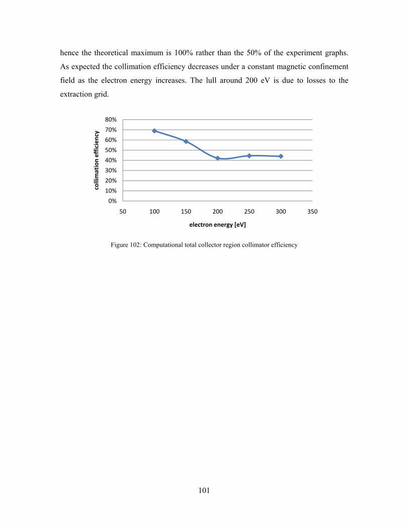
101
hence the theoretical maximum is 100% rather than the 50% of the experiment graphs.
As expected the collimation efficiency decreases under a constant magnetic confinement
field as the electron energy increases. The lull around 200 eV is due to losses to the
extraction grid.
Figure 102: Computational total collector region collimator efficiency
0%
10%
20%
30%
40%
50%
60%
70%
80%
50 100 150 200 250 300 350
collimation efficiency
electron energy [eV]
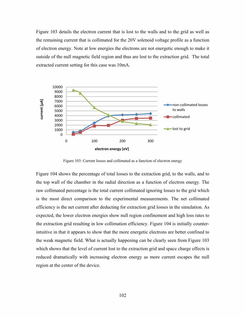
102
Figure 103 details the electron current that is lost to the walls and to the grid as well as
the remaining current that is collimated for the 20V solenoid voltage profile as a function
of electron energy. Note at low energies the electrons are not energetic enough to make it
outside of the null magnetic field region and thus are lost to the extraction grid. The total
extracted current setting for this case was 10mA.
Figure 103: Current losses and collimated as a function of electron energy
Figure 104 shows the percentage of total losses to the extraction grid, to the walls, and to
the top wall of the chamber in the radial direction as a function of electron energy. The
raw collimated percentage is the total current collimated ignoring losses to the grid which
is the most direct comparison to the experimental measurements. The net collimated
efficiency is the net current after deducting for extraction grid losses in the simulation. As
expected, the lower electron energies show null region confinement and high loss rates to
the extraction grid resulting in low collimation efficiency. Figure 104 is initially counter-
intuitive in that it appears to show that the more energetic electrons are better confined to
the weak magnetic field. What is actually happening can be clearly seen from Figure 103
which shows that the level of current lost to the extraction grid and space charge effects is
reduced dramatically with increasing electron energy as more current escapes the null
region at the center of the device.
0100020003000400050006000700080009000
10000
0 100 200 300
curren
t [μA
]
electron energy [eV]
non‐collimated losses to walls
collimated
lost to grid

103
Figure 104: Computational collimator efficiency accounting for extraction grid losses & neglecting losses to extraction grid
0%
10%
20%
30%
40%
50%
60%
70%
80%
90%
100%
0 50 100 150 200 250 300
raw collimated
net collimated
grid losses
total wall losses
top wall losses

104
7.8 SansStabilization Coil Scenario Simulation Results This section details the computational results for the magnetic coil configuration without
the stabilization coil. From Figure 105 we can see that for 300 eV electrons peak current
is obtained near the 20 Volt solenoid profile rather than the 100 and 200 Ampere-Turn
cases (equivalent to 0.64 and 1.70 Volt Solenoid profiles) found by Nieto24. It would
however be improper to say that the true peak is at the 20 Volt solenoid profile as one
would expect greater collection of current and thus higher collimation for increasingly
higher magnetic fields.
Figure 105: Computational collector currents versus solenoidal voltage scaling for 300 eV electrons
A look at Figure 106 shows that not only does the collector current from Figure 105 drop
off at the higher solenoid voltage profiles, but the total current lost to the walls also drops
off. The proper conclusion is that due to the increased confinement in the magnetic null
region more current is lost back to the extraction grid and Child’s law effects.
0
200
400
600
800
1000
1200
1400
1600
1800
2000
5 10 15 20 25
Collector Current [μ
A]
Vsolenoid [V]
1st
2nd
3rd
4th

105
Figure 106: Electron current losses to chamber wall for different solenoid voltage profiles where TW are current losses to the radial chamber wall, and LW & RW represent losses to the left and right axial chamber walls. Grid losses are those to the extraction grid and space charge limit
Figure 107 shows the losses to the extraction grid, radial chamber wall and total wall
losses. It also shows the collimator efficiency computed by summing the current from the
collectors and dividing by the raw extracted current in order to provide a direct
comparison of the collimator efficiency with the experimentally calculated collimator
efficiency which did not account for losses to the extraction grid and space charge
effects. It was observed that peak efficiency in collimation occurred near the 20V
solenoid magnetic profile followed by a steep drop off afterward. This is because the
field is strong enough to confine the electrons in the null region those increasing losses to
the extraction grid.
0
1000
2000
3000
4000
5000
6000
7000
8000
9000
5 10 15 20 25
elen
tron
current [μ
A]
solenoid voltage profile [V]
TW
LW
RW
wall losses
grid losses
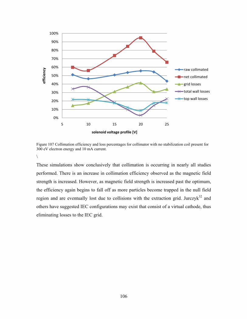
106
Figure 107 Collimation efficiency and loss percentages for collimator with no stabilization coil present for 300 eV electron energy and 10 mA current.
\
These simulations show conclusively that collimation is occurring in nearly all studies
performed. There is an increase in collimation efficiency observed as the magnetic field
strength is increased. However, as magnetic field strength is increased past the optimum,
the efficiency again begins to fall off as more particles become trapped in the null field
region and are eventually lost due to collisions with the extraction grid. Jurczyk32 and
others have suggested IEC configurations may exist that consist of a virtual cathode, thus
eliminating losses to the IEC grid.
0%
10%
20%
30%
40%
50%
60%
70%
80%
90%
100%
5 10 15 20 25
efficiency
solenoid voltage profile [V]
raw collimated
net collimated
grid losses
total wall losses
top wall losses

107
Chapter 8 Conclusions & Future Work
In order to determine the engineering feasibility of a full-scale proton collimator, we have
designed and built a much more economical electron collimator simulation device
supplemented by numerical simulation codes generated in XOOPIC/OOPIC Pro. These
experiments validate the hexapole magnetic confinement concept as a potentially
successful component of a IEC fusion spacecraft power and propulsion source. As a
result, the main and most important objectives of our program were successful, that is,
collimation of electrons from an isotropic source has been observed.
• True collimation of 300 eV electrons without a stabilization coil was demonstrated numerically to approach 95% at a profile corresponding to Vsolenoid = 20.0V, Ifloating = 2.78A, Isolenoid = 4.05A • True collimation of electrons with stabilization coil present was demonstrated numerically to reach 69% at a profile corresponding to Vsolenoid = 7.0V, Istab = 1.1A, Ifloating = 1.1A, Isolenoid = 1.45A • Experimental collimation of electrons with stabilization coil present was demonstrated experimentally to be 35% at 100 eV and reach a peak of 39.6% at 50eV with a profile corresponding to Vsolenoid = 7.0V, Istab = 1.1A, Ifloating = 1.1A, Isolenoid = 1.45A • Experimental collimation of 300 eV electrons without a stabilization coil was demonstrated experimentally to approach 49% at a profile corresponding to Vsolenoid = 20.0V, Ifloating = 2.78A, Isolenoid = 4.05A

108
Figure 108: Comparison of collimation efficiency for computational and experimental cases.
Figure 109: Computational collector plate region electron current components for 300 eV electrons for various solenoid voltage parameters
0%
5%
10%
15%
20%
25%
30%
35%
40%
45%
50%
0 100 200 300 400 500
efficiency
electron energy [eV]
computational
uncollimated
collimated
0
500
1000
1500
2000
2500
3000
5 10 15 20 25
electron
current [μ
A]
solenoid voltage scaling parameter [V]
Iz
Ir
Iphi
total

109
Figure 110: Computational wall losses varying electron energies with the stabilization coil and current profile of Vsolenoid = 7.0V, Istab = 1.1A, Ifloating = 1.1A, Isolenoid = 1.45A
At a solenoid voltage profile of 7 Volts, 100 eV electrons are collimated with wall and
perpendicular component losses of 31%. Increasing the electron energy beyond 100 eV
increases the wall losses by 25% at 300 eV.
Using these experiments as a baseline scaling, 9.5 MAT/m would be required to
collimate 14.7 MeV fusion protons from d-3He fueled IEC fusion core.
Optimization studies on solenoid coil currents are necessary to better refine the non-linear
scaling relationship as well as geometry of the coil configurations to improve the
collimation efficiency further with the presence of the stabilization coil.
6.4% of the 300eV electrons’ initial velocity is directed to the collector plates. The
remaining electrons are trapped by the collimator’s magnetic field. These particles
oscillate around the null field region several hundred times and eventually escape to the
collector plates.
• As particle energy increases, the chamber wall losses increases and collimation
efficiency decreases.
0%
10%
20%
30%
40%
50%
60%
70%
50 100 150 200 250 300 350
wall losses
electron energy [eV]

110
• Collimation is structurally stable and insensitive to perturbations of the particle
source position.
• There are greater particle losses observed with the inclusion of the stabilization
coil at the midpoint of the chamber. Further study could reveal an improved
geometry that would increase collimation efficiency.
• The short length of solenoid coil (using only 1 meter of solenoid coils on a two
meter chamber leaving a higher number of open magnetic field lines) decreased the
collimation efficiency due to chamber wall losses. Further studies are needed to
adequately determine exactly how solenoid coil length affects collimation
efficiency.
• In contrast with the initial electron collimator scaling estimate, a much larger
current on the solenoid coil will be needed on a full scale proton collimator. The
scaling relation needs to be better determined by using more data points to
determine particle energy reaching the collectors.
• The reverse-mode configuration experiments were inadequate to properly
determine if particles can be uncollimated in a similar manner.
Nevertheless, several issues remain for future study.
Additional laboratory experiments are necessary to accurately determine the net current
that escapes past the extraction grid for a range of electron energies and coil current
profiles.
Further laboratory experiments for 300 eV electrons should be conducted while biasing
the collector plates to accurately determine the energy profile of the collimated electrons
reaching the collector plates.
Additional computational work should substitute a plasma source instead of a variable
weight emitter to reduce the effects of space charge losses and losses due to collisions
with the extraction grid.

111
A computational simulation should be undertaken using the output collimation profile as
an input for noble gas mixing with argon and xenon to determine potential thrust and Isp
characteristics for application as a direct energy propulsion device.

112
Appendix A: BiotSavart Base Input File Info {BiotSavart 4.1 data file} Current { name {Current} supplies { { {FloatingSupply} {-2250000} } { {StabilizationSupply} {781100} } { {SolenoidalSupply} {762000} } } } Loop { name {HelmholtzLoop} color 19660 45874 45874 currentSupply FloatingSupply wireDiameter 75 winding 0 nPhi 30 loops { {{1500} {750} {1}} {{1500} {-750} {1}} } nZeta 30 fluxPhiSteps 16 } Solenoid { name {SolenoidCoil} color 19660 45874 45874 currentSupply SolenoidalSupply winding 1 nPhi 30 resolution 1000 autoResolution innerRadius 2100 outerRadius 2110 length 10000 fluxPhiSteps 16 } Tracer { name {TracerProbe} color 65535 65535 0 drawPoint 1 drawFieldLines 1 stepSize 0.01 pathLength 1 }

113
Appendix B: OOPIC Load Input File Subsection VarWeightLoad { units = EV x1MinMKS = 0.4950 x1MaxMKS = 0.5050 x2MinMKS = 0.0000 x2MaxMKS = 0.0025 speciesName = eprotons v1drift = etemp*cos(90*PI/180) v2drift = etemp*sin(90*PI/180) np2c = 1E4 density = 1E12 }

114
Appendix C: OOPIC Base Input File electron_collimator { This is the electron collimator Description block. Below is the graphical description of the physical layout of the experiment * * * * * * * * * * * * * * * * * * * * * **************************************************************************************************** * * * | | | | | | ‐‐‐‐‐‐‐‐‐‐‐‐‐‐‐‐‐‐‐‐‐‐‐‐‐‐‐‐‐‐‐‐‐‐‐‐‐‐‐‐‐‐‐‐‐‐‐‐‐‐‐‐‐‐‐‐‐‐‐‐‐‐‐‐‐‐‐‐‐‐‐‐‐‐‐‐‐‐‐‐‐‐‐‐‐‐‐‐‐‐‐‐‐‐‐‐‐‐‐‐‐‐‐‐‐‐‐‐‐‐‐‐‐‐‐‐‐‐‐‐‐‐‐‐‐‐‐‐‐‐‐‐‐‐‐‐‐‐‐‐‐‐‐‐‐‐‐‐‐‐ FLEXIBLE EXTRACTION CURRENT solenoidal coil ‐ 20 coils, floating coils ‐ 2 coils, stabilization coil ‐ 1 coil, electron source ‐ 100eV AT/m Case ~ V Sol Isol =A Ifir = A Isec =A Collimator8 includes: does not include axial collector plates collector plate current diagnostics } Variables { JMAX = 2000 // number of cells in the z‐direction (x1) KMAX = 600 // number of cells in the r‐direction (x2) solCoilCurrent = 1.45 leftCoilCurrent = ‐1.1 // VARIABLE set from power supply rightCoilCurrent = ‐1.1 // VARIABLE set from power supply stabCoilCurrent = 1.1 // VARIABLE set from power supply leftCoilTurns = 203 // was 189 when shorted rightCoilTurns = 203 stabCoilTurns = 80 solCoilTurns = 24

115
macrodensity = 1.0E4 etemp = 300 // eV PI = 3.1415926 } Region { Grid { J = JMAX // simulation has JMAX cells in z‐direction x1s = 0.0 // start of sim in z is 0 meters x1f = 1 // end of sim in z is 1.0 meters K = KMAX // simulation has KMAX cells in r‐direction x2s = 0.0 // start of sim in r is 0 meters x2f = 0.3 // end of sim in r is 0.3 meters n1 = 1.0 // scaling parameters for non‐uniform grids n2 = 1.0 Geometry = 0 // cylindrical } Control { dt = 1.0E‐12 // simulation time step ElectrostaticFlag = 0 // uses full update of Maxwell's equations (see p36 of OOPIC man) // consider trying flag 1,2,3,&4 if possible StoreTimeHistoryFlag = 1 NonRelativisticFlag = 1 // particles are not relativistic <90% c PlasmaRadiationFlag = 0 // no plasma rad calcs (see page 36 of OOPIC manual) // consider setting flag to 1 if possible } Species { name = eprotons m = 9.11E‐31 q = ‐1.6e‐19 collisionModel=1 // uses electron collision model } //Species //{ // name = ealphas // m = 3.62e‐30 // q = ‐1.6e‐19 // collisionModel=2 //uses ion collision model //} //Species //{ // name = edeuterium // m = 1.82e‐30 // q = ‐1.6e‐19 //} //Species //{ // name = ehelium3 // m = 2.73e‐30 // q = ‐1.6e‐19

116
//} //Species //{ // name = eelectrons // m = 4.96e‐34 // q = 1.6e‐19 //} //PlasmaSource //{ // // enter plasma source stuff here // //} //*********************** Plasma Source ******************************** VarWeightBeamEmitter // P1 ‐ 180 deg { j1 = 950 k1 = 0 j2 = 950 k2 = 1 units = EV normal = ‐1 speciesName = eprotons I = 0.001 // 20 mA halved for symmetry np2c = macrodensity // v1thermal = 300 // should be 300eV when exiting cathode // v2thermal = 0 temperature = etemp v1drift = ‐etemp v2drift = 0 } VarWeightBeamEmitter // P10 ‐ 0 deg { j1 = 1050 k1 = 0 j2 = 1050 k2 = 1 units = EV normal = 1 speciesName = eprotons I = 0.001 // 20 mA halved for symmetry np2c = macrodensity // v1thermal = 300 // should be 300eV when exiting cathode // v2thermal = 0 temperature = etemp v1drift = etemp v2drift = 0 } VarWeightBeamEmitter // P2 ‐ 160 deg { j1 = 952
117
k1 = 14 j2 = 952 k2 = 15 units = EV normal = ‐1 speciesName = eprotons I = 0.001 // 20 mA halved for symmetry np2c = macrodensity // v1thermal = 282 // v2thermal = 103 // should be 300eV when exiting cathode temperature = etemp v1drift = ‐etemp*cos(20*PI/180) // 281.9 v2drift = etemp*sin(160*PI/180) // 102.6 } VarWeightBeamEmitter // P9 ‐ 20 deg { j1 = 1048 k1 = 15 j2 = 1048 k2 = 14 units = EV normal = 1 speciesName = eprotons I = 0.001 // 20 mA halved for symmetry np2c = macrodensity // v1thermal = 282 // v2thermal = 103 // should be 300eV when exiting cathode temperature = etemp v1drift = etemp*cos(20*PI/180) v2drift = etemp*sin(160*PI/180) } VarWeightBeamEmitter // P3 ‐ 140 deg { j1 = 959 k1 = 30 j2 = 959 k2 = 31 units = EV normal = ‐1 speciesName = eprotons I = 0.001 // 20 mA halved for symmetry np2c = macrodensity // v1thermal = 230 // v2thermal = 193 // should be 300eV when exiting cathode temperature = etemp v1drift = ‐etemp*cos(40*PI/180) v2drift = etemp*sin(140*PI/180) } VarWeightBeamEmitter // P8 ‐ 40 deg { j1 = 1041 k1 = 31 j2 = 1041 k2 = 30 units = EV

118
normal = 1 speciesName = eprotons I = 0.001 // 20 mA halved for symmetry np2c = macrodensity // v1thermal = 230 // v2thermal = 193 // should be 300eV when exiting cathode temperature = etemp v1drift = etemp*cos(40*PI/180) v2drift = etemp*sin(140*PI/180) } VarWeightBeamEmitter // P4 ‐ 120 deg { j1 = 971 k1 = 45 j2 = 972 k2 = 45 units = EV normal = 1 speciesName = eprotons I = 0.001 // 20 mA halved for symmetry np2c = macrodensity // v1thermal = 150 // v2thermal = 260 // should be 300eV when exiting cathode temperature = etemp v1drift = ‐etemp*cos(60*PI/180) v2drift = etemp*sin(120*PI/180) } VarWeightBeamEmitter // P7 ‐ 60 deg { j1 = 1028 k1 = 45 j2 = 1029 k2 = 45 units = EV normal = 1 speciesName = eprotons I = 0.001111 // 20 mA halved for symmetry np2c = macrodensity // v1thermal = 150 // v2thermal = 260 // should be 300eV when exiting cathode temperature = etemp v1drift = etemp*cos(60*PI/180) v2drift = etemp*sin(120*PI/180) } VarWeightBeamEmitter // P5 ‐ 100 deg { j1 = 988 k1 = 50 j2 = 989 k2 = 50 units = EV normal = 1 speciesName = eprotons I = 0.001 // 20 mA halved for symmetry np2c = macrodensity

119
// v1thermal = 52 // v2thermal = 295 // should be 300eV when exiting cathode temperature = etemp v1drift = ‐etemp*cos(80*PI/180) v2drift = etemp*sin(100*PI/180) } VarWeightBeamEmitter // P6 ‐ 80 deg { j1 = 1011 k1 = 50 j2 = 1012 k2 = 50 units = EV normal = 1 speciesName = eprotons I = 0.001 // 20 mA halved for symmetry np2c = macrodensity // v1thermal = 52 // v2thermal = 295 // should be 300eV when exiting cathode temperature = etemp v1drift = etemp*cos(80*PI/180) v2drift = etemp*sin(100*PI/180) } Conductor // top of chamber boundary { j1 = 0 // z‐direction k1 = 495 // r‐direction ‐ try 600 j2 = JMAX k2 = 495 // r‐direction ‐ try 600 normal = ‐1 C = 0 } Conductor // right side chamber boundary { j1 = JMAX // z‐direction k1 = 0 // r‐direction j2 = JMAX k2 = 600 normal = ‐1 C = 0 } Conductor // left side chamber boundary { j1 = 0 // z‐direction k1 = 0 // r‐direction j2 = 0 k2 = 600 normal = 1 C = 0 } // *********************** STABILIZATION COIL ********************* CurrentRegion // core coil 8x8 core ‐ 64/80 { j1 = 994 j2 = 1008

120
k1 = 292 k2 = 308 Current = stabCoilCurrent C = stabCoilTurns*64/80 // 80 turns and 64 of 80 turns ratio A = 0 analyticF = 1 direction = 3 } CurrentRegion // top 4x1 core ‐ 4/80 { j1 = 996 j2 = 1004 k1 = 309 k2 = 310 Current = stabCoilCurrent C = stabCoilTurns*4/80 // 80 turns and 4 of 80 turns ratio A = 0 analyticF = 1 direction = 3 } CurrentRegion // right 1x4 core ‐ 4/80 { j1 = 1009 j2 = 1010 k1 = 296 k2 = 304 Current = stabCoilCurrent C = stabCoilTurns*4/80 // 80 turns and 4 of 80 turns ratio A = 0 analyticF = 1 direction = 3 } CurrentRegion // left 1x4 core ‐ 4/80 { j1 = 992 j2 = 993 k1 = 296 k2 = 304 Current = stabCoilCurrent C = stabCoilTurns*4/80 // 80 turns and 4 of 80 turns ratio A = 0 analyticF = 1 direction = 3 } CurrentRegion // bottom 4x1 core ‐ 4/80 { j1 = 996 j2 = 1004 k1 = 290 k2 = 291 Current = stabCoilCurrent C = stabCoilTurns*4/80 // 80 turns and 9 of 177 turns ratio A = 0 analyticF = 1 direction = 3

121
} // ************** RIGHT FLOATING COIL *********************************** CurrentRegion // right floating coil 11x11 core ‐ 121/177 { j1 = 1139 j2 = 1161 k1 = 289 k2 = 311 Current = rightCoilCurrent C = rightCoilTurns*121/177 // 203 turns and 121 of 177 turns ratio A = 0 analyticF = 1 direction = 3 } CurrentRegion // right floating coil top 1x9 core ‐ 9/177 { j1 = 1141 j2 = 1159 k1 = 312 k2 = 313 Current = rightCoilCurrent C = rightCoilTurns*9/177 // 203 turns and 9 of 177 turns ratio A = 0 analyticF = 1 direction = 3 } CurrentRegion // right floating coil top‐top 1x7 core ‐ 7/177 { j1 = 1145 j2 = 1155 k1 = 314 k2 = 315 Current = rightCoilCurrent C = rightCoilTurns*7/177 // 203 turns and 7 of 177 turns ratio A = 0 analyticF = 1 direction = 3 } CurrentRegion // right floating coil bottom 1x9 core ‐ 9/177 { j1 = 1141 j2 = 1159 k1 = 287 k2 = 288 Current = rightCoilCurrent C = rightCoilTurns*9/177 // 203 turns and 9 of 177 turns ratio A = 0 analyticF = 1 direction = 3 } CurrentRegion // right floating coil bottom‐bottom 1x7 core ‐ 7/177 { j1 = 1145 j2 = 1155

122
k1 = 285 k2 = 286 Current = rightCoilCurrent C = rightCoilTurns*7/177 // 203 turns and 7 of 177 turns ratio A = 0 analyticF = 1 direction = 3 } CurrentRegion // right floating coil left 1x9 core ‐ 9/177 { j1 = 1137 j2 = 1138 k1 = 291 k2 = 309 Current = rightCoilCurrent C = rightCoilTurns*9/177 // 203 turns and 9 of 177 turns ratio A = 0 analyticF = 1 direction = 3 } CurrentRegion // right floating coil left‐left 1x7 core ‐ 7/177 { j1 = 1135 j2 = 1136 k1 = 295 k2 = 305 Current = rightCoilCurrent C = rightCoilTurns*7/177 // 203 turns and 7 of 177 turns ratio A = 0 analyticF = 1 direction = 3 } CurrentRegion // right floating coil right 1x9 core ‐ 9/177 { j1 = 1162 j2 = 1163 k1 = 291 k2 = 309 Current = rightCoilCurrent C = rightCoilTurns*9/177 // 203 turns and 9 of 177 turns ratio A = 0 analyticF = 1 direction = 3 } CurrentRegion // right floating coil right‐right 1x7 core ‐ 7/177 { j1 = 1164 j2 = 1165 k1 = 295 k2 = 305 Current = rightCoilCurrent C = rightCoilTurns*7/177 // 203 turns and 7 of 177 turns ratio A = 0 analyticF = 1 direction = 3

123
} // ************** LEFT FLOATING COIL********************* CurrentRegion // left floating coil 11x11 core ‐ 121/177 { j1 = 839 j2 = 861 k1 = 289 k2 = 311 Current = leftCoilCurrent C = leftCoilTurns*121/177 // 203 turns and 121 of 177 turns ratio A = 0 analyticF = 1 direction = 3 } CurrentRegion // left floating coil top 1x9 core ‐ 9/177 { j1 = 841 j2 = 859 k1 = 312 k2 = 313 Current = leftCoilCurrent C = leftCoilTurns*9/177 // 203 turns and 9 of 177 turns ratio A = 0 analyticF = 1 direction = 3 } CurrentRegion // left floating coil top‐top 1x7 core ‐ 7/177 { j1 = 845 j2 = 855 k1 = 314 k2 = 315 Current = leftCoilCurrent C = leftCoilTurns*7/177 // 203 turns and 7 of 177 turns ratio A = 0 analyticF = 1 direction = 3 } CurrentRegion // left floating coil bottom 1x9 core ‐ 9/177 { j1 = 841 j2 = 859 k1 = 287 k2 = 288 Current = leftCoilCurrent C = leftCoilTurns*9/177 // 203 turns and 9 of 177 turns ratio A = 0 analyticF = 1 direction = 3 } CurrentRegion // left floating coil bottom‐bottom 1x7 core ‐ 7/177 { j1 = 845 j2 = 855
124
k1 = 285 k2 = 286 Current = leftCoilCurrent C = leftCoilTurns*7/177 // 203 turns and 7 of 177 turns ratio A = 0 analyticF = 1 direction = 3 } CurrentRegion // left floating coil left 1x9 core ‐ 9/177 { j1 = 837 j2 = 838 k1 = 291 k2 = 309 Current = leftCoilCurrent C = leftCoilTurns*9/177 // 203 turns and 9 of 177 turns ratio A = 0 analyticF = 1 direction = 3 } CurrentRegion // left floating coil left‐left 1x7 core ‐ 7/177 { j1 = 835 j2 = 836 k1 = 295 k2 = 305 Current = leftCoilCurrent C = leftCoilTurns*7/177 // 203 turns and 7 of 177 turns ratio A = 0 analyticF = 1 direction = 3 } CurrentRegion // left floating coil right 1x9 core ‐ 9/177 { j1 = 862 j2 = 863 k1 = 291 k2 = 309 Current = leftCoilCurrent C = leftCoilTurns*9/177 // 203 turns and 9 of 177 turns ratio A = 0 analyticF = 1 direction = 3 } CurrentRegion // left floating coil right‐right 1x7 core ‐ 7/177 { j1 = 864 j2 = 865 k1 = 295 k2 = 305 Current = leftCoilCurrent C = leftCoilTurns*7/177 // 203 turns and 7 of 177 turns ratio A = 0 analyticF = 1 direction = 3

125
} // ******************** SOLENOIDAL COILS************************************* CurrentRegion // solenid coil 01 { j1 = 36 j2 = 65 k1 = 580 k2 = 599 Current = solCoilCurrent C = solCoilTurns // 24 turns A = 0 analyticF = 1 direction = 3 } CurrentRegion // solenoid coil 02 { j1 = 136 j2 = 165 k1 = 580 k2 = 599 Current = solCoilCurrent C = solCoilTurns // 24 turns A = 0 analyticF = 1 direction = 3 } CurrentRegion // solenoid coil 03 { j1 = 236 j2 = 265 k1 = 580 k2 = 599 Current = solCoilCurrent C = solCoilTurns // 24 turns A = 0 analyticF = 1 direction = 3 } CurrentRegion // solenoid coil 04 { j1 = 336 j2 = 365 k1 = 580 k2 = 599 Current = solCoilCurrent C = solCoilTurns // 24 turns A = 0 analyticF = 1 direction = 3 } CurrentRegion // solenoid coil 05 { j1 = 436 j2 = 465 k1 = 580

126
k2 = 599 Current = solCoilCurrent C = solCoilTurns // 24 turns A = 0 analyticF = 1 direction = 3 } CurrentRegion // solenoid coil 06 { j1 = 536 j2 = 565 k1 = 580 k2 = 599 Current = solCoilCurrent C = solCoilTurns // 24 turns A = 0 analyticF = 1 direction = 3 } CurrentRegion // solenoid coil 07 { j1 = 636 j2 = 665 k1 = 580 k2 = 599 Current = solCoilCurrent C = solCoilTurns // 24 turns A = 0 analyticF = 1 direction = 3 } CurrentRegion // solenoid coil 08 { j1 = 736 j2 = 765 k1 = 580 k2 = 599 Current = solCoilCurrent C = solCoilTurns // 24 turns A = 0 analyticF = 1 direction = 3 } CurrentRegion // solenoid coil 09 { j1 = 836 j2 = 865 k1 = 580 k2 = 599 Current = solCoilCurrent C = solCoilTurns // 24 turns A = 0 analyticF = 1 direction = 3 }

127
CurrentRegion // solenoid coil 10 { j1 = 936 j2 = 965 k1 = 580 k2 = 599 Current = solCoilCurrent C = solCoilTurns // 24 turns A = 0 analyticF = 1 direction = 3 } CurrentRegion // solenoid coil 11 { j1 = 1036 j2 = 1065 k1 = 580 k2 = 599 Current = solCoilCurrent C = solCoilTurns // 24 turns A = 0 analyticF = 1 direction = 3 } CurrentRegion // solenoid coil 12 { j1 = 1136 j2 = 1165 k1 = 580 k2 = 599 Current = solCoilCurrent C = solCoilTurns // 24 turns A = 0 analyticF = 1 direction = 3 } CurrentRegion // solenoid coil 13 { j1 = 1236 j2 = 1265 k1 = 580 k2 = 599 Current = solCoilCurrent C = solCoilTurns // 24 turns A = 0 analyticF = 1 direction = 3 } CurrentRegion // solenoid coil 14 { j1 = 1336 j2 = 1365 k1 = 580 k2 = 599

128
Current = solCoilCurrent C = solCoilTurns // 24 turns A = 0 analyticF = 1 direction = 3 } CurrentRegion // solenoid coil 15 { j1 = 1436 j2 = 1465 k1 = 580 k2 = 599 Current = solCoilCurrent C = solCoilTurns // 24 turns A = 0 analyticF = 1 direction = 3 } CurrentRegion // solenoid coil 16 { j1 = 1536 j2 = 1565 k1 = 580 k2 = 599 Current = solCoilCurrent C = solCoilTurns // 24 turns A = 0 analyticF = 1 direction = 3 } CurrentRegion // solenoid coil 17 { j1 = 1636 j2 = 1665 k1 = 580 k2 = 599 Current = solCoilCurrent C = solCoilTurns // 24 turns A = 0 analyticF = 1 direction = 3 } CurrentRegion // solenoid coil 18 { j1 = 1736 j2 = 1765 k1 = 580 k2 = 599 Current = solCoilCurrent C = solCoilTurns // 24 turns A = 0 analyticF = 1 direction = 3 } CurrentRegion // solenoid coil 19

129
{ j1 = 1836 j2 = 1865 k1 = 580 k2 = 599 Current = solCoilCurrent C = solCoilTurns // 24 turns A = 0 analyticF = 1 direction = 3 } CurrentRegion // solenoid coil 20 { j1 = 1936 j2 = 1965 k1 = 580 k2 = 599 Current = solCoilCurrent C = solCoilTurns // 24 turns A = 0 analyticF = 1 direction = 3 } CylindricalAxis { j1 = 0 // z‐direction k1 = 0 // r‐direction j2 = JMAX k2 = 0 normal = 1 } ExitPort { // A boundary where electromagnetic waves can exit the grid, with minimal reflection j1 = 0 // z‐direction k1 = KMAX // r‐direction j2 = JMAX k2 = KMAX normal = ‐1 } //********************AXIAL COLLECTOR PLATE DIAGNOSTICS******************* //****************************** I1 = Iz ****************************** Diagnostic // Center axial collector Iz { HistMax = 100 Comb = 1 Ave = 0 j1 = 1790 // z‐direction k1 = 0 // r‐direction ‐ 0 cm j2 = 1790 k2 = 100 // r‐direction ‐ 5 cm VarName = I1

130
title = 1st Axial Collector v Iz // grounded collector x1_Label = r x2_Label = time save = 1 } Diagnostic // 2nd axial collector Iz { HistMax = 100 Comb = 1 Ave = 0 j1 = 1790 // z‐direction k1 = 140 // r‐direction ‐ 0 cm j2 = 1790 k2 = 172 // r‐direction ‐ 5 cm VarName = I1 title = 2nd Axial Collector v Iz // grounded collector x1_Label = r x2_Label = time save = 1 } Diagnostic // 3rd axial collector Iz { HistMax = 100 Comb = 1 Ave = 0 j1 = 1790 // z‐direction k1 = 198 // r‐direction ‐ 0 cm j2 = 1790 k2 = 222 // r‐direction ‐ 5 cm VarName = I1 title = 3rd Axial Collector v Iz // grounded collector x1_Label = r x2_Label = time save = 1 } Diagnostic // 4th axial collector Iz { HistMax = 100 Comb = 1 Ave = 0 j1 = 1790 // z‐direction k1 = 242 // r‐direction ‐ 0 cm j2 = 1790 k2 = 262 // r‐direction ‐ 5 cm VarName = I1 title = 4th Axial Collector v Iz // grounded collector x1_Label = r x2_Label = time save = 1 } //****************************Axial I2 = Ir************************* Diagnostic // Center axial collector Ir { HistMax = 100 Comb = 1

131
Ave = 0 j1 = 1790 // z‐direction k1 = 0 // r‐direction ‐ 0 cm j2 = 1790 k2 = 100 // r‐direction ‐ 5 cm VarName = I2 title = 1st Axial Collector v Ir // grounded collector x1_Label = r x2_Label = time save = 1 } Diagnostic // 2nd axial collector Ir { HistMax = 100 Comb = 1 Ave = 0 j1 = 1790 // z‐direction k1 = 140 // r‐direction ‐ 0 cm j2 = 1790 k2 = 172 // r‐direction ‐ 5 cm VarName = I2 title = 2nd Axial Collector v Ir // grounded collector x1_Label = r x2_Label = time save = 1 } Diagnostic // 3rd axial collector Ir { HistMax = 100 Comb = 1 Ave = 0 j1 = 1790 // z‐direction k1 = 198 // r‐direction ‐ 0 cm j2 = 1790 k2 = 222 // r‐direction ‐ 5 cm VarName = I2 title = 3rd Axial Collector v Ir // grounded collector x1_Label = r x2_Label = time save = 1 } Diagnostic // 4th axial collector Ir { HistMax = 100 Comb = 1 Ave = 0 j1 = 1790 // z‐direction k1 = 242 // r‐direction ‐ 0 cm j2 = 1790 k2 = 262 // r‐direction ‐ 5 cm VarName = I2 title = 4th Axial Collector v Ir // grounded collector x1_Label = r x2_Label = time
132
save = 1 } //********************composite collector *************************** Diagnostic // Composite for Iz collector { HistMax = 100 Comb = 1 Ave = 0 j1 = 1790 // z‐direction k1 = 0 // r‐direction ‐ 0 cm j2 = 1790 k2 = 262 // r‐direction ‐ 13.1 cm VarName = I1 title = Full Axial Collector v Iz // grounded collector x1_Label = r x2_Label = time save = 1 } Diagnostic // Composite for Ir { HistMax = 1000 Comb = 1 Ave = 0 j1 = 1790 // z‐direction k1 = 0 // r‐direction ‐ 0 cm j2 = 1790 k2 = 262 // r‐direction ‐ 13.1 cm VarName = I2 title = Full Axial Collector v Ir // grounded collector x1_Label = r x2_Label = time save = 1 } Diagnostic // Composite for Iphi { HistMax = 100 Comb = 1 Ave = 0 j1 = 1790 // z‐direction k1 = 0 // r‐direction ‐ 0 cm j2 = 1790 k2 = 262 // r‐direction ‐ 13.1 cm VarName = I3 title = Full Axial Collector v Iphi // grounded collector x1_Label = r x2_Label = time save = 1 } Diagnostic // top of chamber boundary Iz { HistMax = 100 Comb = 1 Ave = 0 j1 = 0 // z‐direction k1 = 490 // top wall at 495
133
j2 = JMAX k2 = 490 // top wall at 495 VarName = I1 title = Iz Current Losses to Top Chamber Wall x1_Label = z x2_Label = time save = 1 } Diagnostic // top of chamber boundary Ir { HistMax = 100 Comb = 1 Ave = 0 j1 = 0 // z‐direction k1 = 490 // top wall at 495 j2 = JMAX k2 = 490 // top wall at 495 VarName = I2 title = Ir Current Losses to Top Chamber Wall x1_Label = z x2_Label = time save = 1 } Diagnostic // top of chamber boundary Iphi { HistMax = 100 Comb = 1 Ave = 0 j1 = 0 // z‐direction k1 = 490 // top wall at 495 j2 = JMAX k2 = 490 // top wall at 495 VarName = I3 title = Iphi Current Losses to Top Chamber Wall x1_Label = z x2_Label = time save = 1 } Diagnostic // losses to left coil Iz { HistMax = 100 Comb = 1 Ave =0 j1 = 835 // z‐direction k1 = 295 // r‐direction j2 = 865 k2 = 295 VarName = I1 title = Iz losses to left coil x1_Label = z x2_Label = time save = 1 } Diagnostic // losses to right coil Iz {

134
HistMax = 100 Comb = 1 Ave =0 j1 = 1135 // z‐direction k1 = 295 // r‐direction j2 = 1165 k2 = 295 VarName = I1 title = Iz losses to right coil x1_Label = z x2_Label = time save = 1 } Diagnostic // losses to left coil Ir { HistMax = 100 Comb = 1 Ave =0 j1 = 835 // z‐direction k1 = 295 // r‐direction j2 = 865 k2 = 295 VarName = I2 title = Ir losses to left coil x1_Label = z x2_Label = time save = 1 } Diagnostic // losses to right coil Ir { HistMax = 100 Comb = 1 Ave =0 j1 = 1135 // z‐direction k1 = 295 // r‐direction j2 = 1165 k2 = 295 VarName = I2 title = Ir losses to right coil x1_Label = z x2_Label = time save = 1 } Diagnostic // losses to stab coil Iz { HistMax = 100 Comb = 1 Ave =0 j1 = 990 // z‐direction k1 = 295 // r‐direction j2 = 1010 k2 = 295 VarName = I1 title = Iz losses to stab coil x1_Label = z
135
x2_Label = time save = 1 } Diagnostic // losses to stab coil Ir { HistMax = 100 Comb = 1 Ave =0 j1 = 990 // z‐direction k1 = 295 // r‐direction j2 = 1010 k2 = 295 VarName = I2 title = Ir losses to stab coil x1_Label = z x2_Label = time save = 1 } Diagnostic // losses to left side of chamber Iz { HistMax = 100 Comb = 1 Ave =0 j1 = 5 // z‐direction k1 = 0 // r‐direction j2 = 5 // left wall at 0 k2 = 495 VarName = I1 title = Iz losses to left chamber wall x1_Label = z x2_Label = time save = 1 } Diagnostic // losses to left side of chamber Ir { HistMax = 100 Comb = 1 Ave =0 j1 = 5 // z‐direction k1 = 0 // r‐direction j2 = 5 // left wall at 0 k2 = 495 VarName = I2 title = Ir losses to left chamber wall x1_Label = z x2_Label = time save = 1 } Diagnostic // losses to left side of chamber Iphi { HistMax = 100 Comb = 1 Ave =0 j1 = 5 // z‐direction k1 = 0 // r‐direction

136
j2 = 5 // left wall at 0 k2 = 495 VarName = I3 title = Iphi losses to left chamber wall x1_Label = z x2_Label = time save = 1 } Diagnostic // losses to right chamber wall Iz { HistMax = 100 Comb = 1 Ave =0 j1 = 1995 // z‐direction k1 = 0 // r‐direction j2 = 1995 // right wall at 2000 k2 = 495 // top wall at 495 VarName = I1 title = Iz losses to right chamber wall x1_Label = z x2_Label = time save = 1 } Diagnostic // losses to right chamber wall Ir { HistMax = 100 Comb = 1 Ave =0 j1 = 1995 // z‐direction k1 = 0 // r‐direction j2 = 1995 // right wall at 2000 k2 = 495 // top wall at 495 VarName = I2 title = Ir losses to right chamber wall x1_Label = z x2_Label = time save = 1 } Diagnostic // losses to right chamber wall Iphi { HistMax = 100 Comb = 1 Ave =0 j1 = 1995 // z‐direction k1 = 0 // r‐direction j2 = 1995 // right wall at 2000 k2 = 495 // top wall at 495 VarName = I3 title = Iphi losses to right chamber wall x1_Label = z x2_Label = time save = 1 } //*****************H5 AXIAL COLLECTOR PLATE DIAGNOSTICS*****************

137
//*************************************************************************** H5Diagnostic { VarName = avgKE_species dumpPeriod = 0 fileName = DiagResults_2Proc } H5Diagnostic { VarName = nphysical_particle dumpPeriod = 0 fileName = DiagResults_2Proc } H5Diagnostic { VarName = ncomputer_particle dumpPeriod = 0 fileName = DiagResults_2Proc } }

138
Appendix D: Electron Gun Additions to OOPIC Input File Variables { acDistance = 29 // 12mm (24), 14.5mm (29), 17mm (34), 19.5mm (39) } //***********************Electron Gun Setup************************* VarWeightBeamEmitter // electron gun emitter { j1 = 202 k1 = 0 j2 = 202 k2 = 8 units = EV normal = 1 speciesName = eprotons I = 0.0045 // 9 mA halved for symmetry np2c = macrodensity v1drift = 300 // should be 120eV when exiting cathode } //************************ ANODE *********************************** Equipotential // electron gun anode - left { j1 = 200 + acDistance k1 = 10 j2 = 200 + acDistance k2 = 51 normal = 1 C = 0 } Equipotential // electron gun anode - right { j1 = 200 + acDistance + 10 k1 = 10 j2 = 200 + acDistance + 10 k2 = 51 normal = 1 C = 0 } Equipotential // electron gun anode - bottom { j1 = 200 + acDistance k1 = 10 j2 = 200 + acDistance + 10 k2 = 10 normal = 1 C = 0 }

139
Equipotential // electron gun anode - top { j1 = 200 + acDistance k1 = 51 j2 = 200 + acDistance + 10 k2 = 51 normal = 1 C = 0 } //************************* CATHODE ******************************* Equipotential // electron gun cathode -300V left { j1 = 200 // z-direction k1 = 10 // r-direction j2 = 216 k2 = 51 normal = 1 C = -300 } Equipotential // electron gun cathode -300V right { j1 = 190 // z-direction k1 = 10 // r-direction j2 = 206 k2 = 51 normal = 1 C = -300 } Equipotential // electron gun cathode -300V top { j1 = 206 // z-direction k1 = 51 // r-direction j2 = 216 k2 = 51 normal = 1 C = -300 } Equipotential // electron gun cathode -300V botton { j1 = 190 // z-direction k1 = 10 // r-direction j2 = 200 k2 = 10 normal = 1 C = -300 } //********************* END ELECTRON GUN ******************************

140
Appendix E: Double Collimator OOPIC Input File electron_collimator { This is the electron collimator Description block. Below is the graphical description of the physical layout of the experiment * * * * * * * * * * * * * * * * * * * * * **************************************************************************************************** * * * | | | | | | ------------------------------------------------------------------------------------------------------------------------------------------------------ FLEXIBLE EXTRACTION CURRENT solenoidal coil - 20 coils, floating coils - 2 coils, stabilization coil - 1 coil, electron source - 100eV AT/m Case ~ V Sol Isol =A Ifir = A Isec =A Collimator20 includes: does not include axial collector plates collector plate current diagnostics } Variables { JMAX = 4000 // number of cells in the z-direction (x1) KMAX = 600 // number of cells in the r-direction (x2) solCoilCurrent = 4.06 leftCoilCurrent = -2.85 // VARIABLE set from power supply rightCoilCurrent = -2.85 // VARIABLE set from power supply stabCoilCurrent = 2.85 // VARIABLE set from power supply leftCoilTurns = 203 // was 189 when shorted rightCoilTurns = 203

141
stabCoilTurns = 80 solCoilTurns = 24 macrodensity = 1.0E4 etemp = 300 // eV PI = 3.1415926 } Region { Grid { J = JMAX // simulation has JMAX cells in z-direction x1s = 0.0 // start of sim in z is 0 meters x1f = 1 // end of sim in z is 1.0 meters K = KMAX // simulation has KMAX cells in r-direction x2s = 0.0 // start of sim in r is 0 meters x2f = 0.3 // end of sim in r is 0.3 meters n1 = 1.0 // scaling parameters for non-uniform grids n2 = 1.0 Geometry = 0 // cylindrical } Control { dt = 5.0E-13 // simulation time step ElectrostaticFlag = 0 // uses full update of Maxwell's equations (see p36 of OOPIC man) // consider trying flag 1,2,3,&4 if possible StoreTimeHistoryFlag = 1 NonRelativisticFlag = 1 // particles are not relativistic <90% c PlasmaRadiationFlag = 0 // no plasma rad calcs (see page 36 of OOPIC manual) // consider setting flag to 1 if possible } Species { name = eprotons m = 9.11E-31 q = -1.6e-19 collisionModel=1 // uses electron collision model } //Species //{ // name = ealphas // m = 3.62e-30 // q = -1.6e-19 // collisionModel=2 //uses ion collision model //} //Species //{ // name = edeuterium // m = 1.82e-30 // q = -1.6e-19 //} //Species //{ // name = ehelium3 // m = 2.73e-30
142
// q = -1.6e-19 //} //Species //{ // name = eelectrons // m = 4.96e-34 // q = 1.6e-19 //} //*********************** Plasma Source 1***************************** VarWeightBeamEmitter // P1 - 180 deg { j1 = 950 k1 = 0 j2 = 950 k2 = 1 units = EV normal = -1 speciesName = eprotons I = 0.001 // 20 mA halved for symmetry np2c = macrodensity // v1thermal = 300 // should be 300eV when exiting cathode // v2thermal = 0 temperature = etemp v1drift = -etemp v2drift = 0 } VarWeightBeamEmitter // P10 - 0 deg { j1 = 1050 k1 = 0 j2 = 1050 k2 = 1 units = EV normal = 1 speciesName = eprotons I = 0.001 // 20 mA halved for symmetry np2c = macrodensity // v1thermal = 300 // should be 300eV when exiting cathode // v2thermal = 0 temperature = etemp v1drift = etemp v2drift = 0 } VarWeightBeamEmitter // P2 - 160 deg { j1 = 952 k1 = 14 j2 = 952 k2 = 15 units = EV normal = -1 speciesName = eprotons I = 0.001 // 20 mA halved for symmetry np2c = macrodensity

143
// v1thermal = 282 // v2thermal = 103 // should be 300eV when exiting cathode temperature = etemp v1drift = -etemp*cos(20*PI/180) // 281.9 v2drift = etemp*sin(160*PI/180) // 102.6 } VarWeightBeamEmitter // P9 - 20 deg { j1 = 1048 k1 = 15 j2 = 1048 k2 = 14 units = EV normal = 1 speciesName = eprotons I = 0.001 // 20 mA halved for symmetry np2c = macrodensity // v1thermal = 282 // v2thermal = 103 // should be 300eV when exiting cathode temperature = etemp v1drift = etemp*cos(20*PI/180) v2drift = etemp*sin(160*PI/180) } VarWeightBeamEmitter // P3 - 140 deg { j1 = 959 k1 = 30 j2 = 959 k2 = 31 units = EV normal = -1 speciesName = eprotons I = 0.001 // 20 mA halved for symmetry np2c = macrodensity // v1thermal = 230 // v2thermal = 193 // should be 300eV when exiting cathode temperature = etemp v1drift = -etemp*cos(40*PI/180) v2drift = etemp*sin(140*PI/180) } VarWeightBeamEmitter // P8 - 40 deg { j1 = 1041 k1 = 31 j2 = 1041 k2 = 30 units = EV normal = 1 speciesName = eprotons I = 0.001 // 20 mA halved for symmetry np2c = macrodensity // v1thermal = 230 // v2thermal = 193 // should be 300eV when exiting cathode temperature = etemp v1drift = etemp*cos(40*PI/180) v2drift = etemp*sin(140*PI/180) }
144
VarWeightBeamEmitter // P4 - 120 deg { j1 = 971 k1 = 45 j2 = 972 k2 = 45 units = EV normal = 1 speciesName = eprotons I = 0.001 // 20 mA halved for symmetry np2c = macrodensity // v1thermal = 150 // v2thermal = 260 // should be 300eV when exiting cathode temperature = etemp v1drift = -etemp*cos(60*PI/180) v2drift = etemp*sin(120*PI/180) } VarWeightBeamEmitter // P7 - 60 deg { j1 = 1028 k1 = 45 j2 = 1029 k2 = 45 units = EV normal = 1 speciesName = eprotons I = 0.001111 // 20 mA halved for symmetry np2c = macrodensity // v1thermal = 150 // v2thermal = 260 // should be 300eV when exiting cathode temperature = etemp v1drift = etemp*cos(60*PI/180) v2drift = etemp*sin(120*PI/180) } VarWeightBeamEmitter // P5 - 100 deg { j1 = 988 k1 = 50 j2 = 989 k2 = 50 units = EV normal = 1 speciesName = eprotons I = 0.001 // 20 mA halved for symmetry np2c = macrodensity // v1thermal = 52 // v2thermal = 295 // should be 300eV when exiting cathode temperature = etemp v1drift = -etemp*cos(80*PI/180) v2drift = etemp*sin(100*PI/180) } VarWeightBeamEmitter // P6 - 80 deg { j1 = 1011 k1 = 50 j2 = 1012 k2 = 50
145
units = EV normal = 1 speciesName = eprotons I = 0.001 // 20 mA halved for symmetry np2c = macrodensity // v1thermal = 52 // v2thermal = 295 // should be 300eV when exiting cathode temperature = etemp v1drift = etemp*cos(80*PI/180) v2drift = etemp*sin(100*PI/180) } //************************* Plasma Source 2 *************************** VarWeightBeamEmitter // P1 - 180 deg { j1 = 950+2000 k1 = 0 j2 = 950+2000 k2 = 1 units = EV normal = -1 speciesName = eprotons I = 0.001 // 20 mA halved for symmetry np2c = macrodensity // v1thermal = 300 // should be 300eV when exiting cathode // v2thermal = 0 temperature = etemp v1drift = -etemp v2drift = 0 } VarWeightBeamEmitter // P10 - 0 deg { j1 = 1050+2000 k1 = 0 j2 = 1050+2000 k2 = 1 units = EV normal = 1 speciesName = eprotons I = 0.001 // 20 mA halved for symmetry np2c = macrodensity // v1thermal = 300 // should be 300eV when exiting cathode // v2thermal = 0 temperature = etemp v1drift = etemp v2drift = 0 } VarWeightBeamEmitter // P2 - 160 deg { j1 = 952+2000 k1 = 14 j2 = 952+2000 k2 = 15 units = EV normal = -1

146
speciesName = eprotons I = 0.001 // 20 mA halved for symmetry np2c = macrodensity // v1thermal = 282 // v2thermal = 103 // should be 300eV when exiting cathode temperature = etemp v1drift = -etemp*cos(20*PI/180) // 281.9 v2drift = etemp*sin(160*PI/180) // 102.6 } VarWeightBeamEmitter // P9 - 20 deg { j1 = 1048+2000 k1 = 15 j2 = 1048+2000 k2 = 14 units = EV normal = 1 speciesName = eprotons I = 0.001 // 20 mA halved for symmetry np2c = macrodensity // v1thermal = 282 // v2thermal = 103 // should be 300eV when exiting cathode temperature = etemp v1drift = etemp*cos(20*PI/180) v2drift = etemp*sin(160*PI/180) } VarWeightBeamEmitter // P3 - 140 deg { j1 = 959+2000 k1 = 30 j2 = 959+2000 k2 = 31 units = EV normal = -1 speciesName = eprotons I = 0.001 // 20 mA halved for symmetry np2c = macrodensity // v1thermal = 230 // v2thermal = 193 // should be 300eV when exiting cathode temperature = etemp v1drift = -etemp*cos(40*PI/180) v2drift = etemp*sin(140*PI/180) } VarWeightBeamEmitter // P8 - 40 deg { j1 = 1041+2000 k1 = 31 j2 = 1041+2000 k2 = 30 units = EV normal = 1 speciesName = eprotons I = 0.001 // 20 mA halved for symmetry np2c = macrodensity // v1thermal = 230 // v2thermal = 193 // should be 300eV when exiting cathode temperature = etemp
147
v1drift = etemp*cos(40*PI/180) v2drift = etemp*sin(140*PI/180) } VarWeightBeamEmitter // P4 - 120 deg { j1 = 971+2000 k1 = 45 j2 = 972+2000 k2 = 45 units = EV normal = 1 speciesName = eprotons I = 0.001 // 20 mA halved for symmetry np2c = macrodensity // v1thermal = 150 // v2thermal = 260 // should be 300eV when exiting cathode temperature = etemp v1drift = -etemp*cos(60*PI/180) v2drift = etemp*sin(120*PI/180) } VarWeightBeamEmitter // P7 - 60 deg { j1 = 1028+2000 k1 = 45 j2 = 1029+2000 k2 = 45 units = EV normal = 1 speciesName = eprotons I = 0.001111 // 20 mA halved for symmetry np2c = macrodensity // v1thermal = 150 // v2thermal = 260 // should be 300eV when exiting cathode temperature = etemp v1drift = etemp*cos(60*PI/180) v2drift = etemp*sin(120*PI/180) } VarWeightBeamEmitter // P5 - 100 deg { j1 = 988+2000 k1 = 50 j2 = 989+2000 k2 = 50 units = EV normal = 1 speciesName = eprotons I = 0.001 // 20 mA halved for symmetry np2c = macrodensity // v1thermal = 52 // v2thermal = 295 // should be 300eV when exiting cathode temperature = etemp v1drift = -etemp*cos(80*PI/180) v2drift = etemp*sin(100*PI/180) } VarWeightBeamEmitter // P6 - 80 deg { j1 = 1011+2000

148
k1 = 50 j2 = 1012+2000 k2 = 50 units = EV normal = 1 speciesName = eprotons I = 0.001 // 20 mA halved for symmetry np2c = macrodensity // v1thermal = 52 // v2thermal = 295 // should be 300eV when exiting cathode temperature = etemp v1drift = etemp*cos(80*PI/180) v2drift = etemp*sin(100*PI/180) } //******************End Plasma Source Section ************************ //****************Chamber Boundary Section *************************** Conductor // top of chamber boundary { j1 = 0 // z-direction k1 = 495 // r-direction - try 600 j2 = JMAX k2 = 495 // r-direction - try 600 normal = -1 C = 0 } Conductor // right side chamber boundary { j1 = JMAX // z-direction k1 = 0 // r-direction j2 = JMAX k2 = KMAX normal = -1 C = 0 } Conductor // left side chamber boundary { j1 = 0 // z-direction k1 = 0 // r-direction j2 = 0 k2 = KMAX normal = 1 C = 0 } Conductor // left horizontal chamber boundary { j1 = 0 // z-direction k1 = 198 // r-direction j2 = 167 k2 = 198 normal = 1 C = 0 } Conductor // left verticle chamber boundary { j1 = 167 // z-direction

149
k1 = 198 // r-direction j2 = 167 k2 = 495 normal = 1 C = 0 } Conductor // center horizontal chamber boundary { j1 = 1934 // z-direction k1 = 198 // r-direction j2 = 2067 k2 = 198 normal = 1 C = 0 } Conductor // left center verticle chamber boundary { j1 = 1934 // z-direction k1 = 198 // r-direction j2 = 1934 k2 = 495 normal = 1 C = 0 } Conductor // right center verticle chamber boundary { j1 = 2067 // z-direction k1 = 198 // r-direction j2 = 2067 k2 = 495 normal = 1 C = 0 } Conductor // right horizontal chamber boundary { j1 = 3834 // z-direction k1 = 198 // r-direction j2 = JMAX k2 = 198 normal = 1 C = 0 } Conductor // right verticle chamber boundary { j1 = 3834 // z-direction k1 = 198 // r-direction j2 = 3834 k2 = 495 normal = 1 C = 0 } // ****************End Chamber Boundary Section *********************** // ***************** STABILIZATION COIL STATION 1 ********************* CurrentRegion // core coil 8x8 core - 64/80 {

150
j1 = 994 j2 = 1008 k1 = 292 k2 = 308 Current = stabCoilCurrent C = stabCoilTurns*64/80 // 80 turns and 64 of 80 turns ratio A = 0 analyticF = 1 direction = 3 } CurrentRegion // top 4x1 core - 4/80 { j1 = 996 j2 = 1004 k1 = 309 k2 = 310 Current = stabCoilCurrent C = stabCoilTurns*4/80 // 80 turns and 4 of 80 turns ratio A = 0 analyticF = 1 direction = 3 } CurrentRegion // right 1x4 core - 4/80 { j1 = 1009 j2 = 1010 k1 = 296 k2 = 304 Current = stabCoilCurrent C = stabCoilTurns*4/80 // 80 turns and 4 of 80 turns ratio A = 0 analyticF = 1 direction = 3 } CurrentRegion // left 1x4 core - 4/80 { j1 = 992 j2 = 993 k1 = 296 k2 = 304 Current = stabCoilCurrent C = stabCoilTurns*4/80 // 80 turns and 4 of 80 turns ratio A = 0 analyticF = 1 direction = 3 } CurrentRegion // bottom 4x1 core - 4/80 { j1 = 996 j2 = 1004 k1 = 290 k2 = 291 Current = stabCoilCurrent C = stabCoilTurns*4/80 // 80 turns and 9 of 177 turns ratio A = 0

151
analyticF = 1 direction = 3 } // ******************************* STABILIZATION COIL STATION 2 *********************************** CurrentRegion // core coil 8x8 core - 64/80 { j1 = 994+2000 j2 = 1008+2000 k1 = 292 k2 = 308 Current = stabCoilCurrent C = stabCoilTurns*64/80 // 80 turns and 64 of 80 turns ratio A = 0 analyticF = 1 direction = 3 } CurrentRegion // top 4x1 core - 4/80 { j1 = 996+2000 j2 = 1004+2000 k1 = 309 k2 = 310 Current = stabCoilCurrent C = stabCoilTurns*4/80 // 80 turns and 4 of 80 turns ratio A = 0 analyticF = 1 direction = 3 } CurrentRegion // right 1x4 core - 4/80 { j1 = 1009+2000 j2 = 1010+2000 k1 = 296 k2 = 304 Current = stabCoilCurrent C = stabCoilTurns*4/80 // 80 turns and 4 of 80 turns ratio A = 0 analyticF = 1 direction = 3 } CurrentRegion // left 1x4 core - 4/80 { j1 = 992+2000 j2 = 993+2000 k1 = 296 k2 = 304 Current = stabCoilCurrent C = stabCoilTurns*4/80 // 80 turns and 4 of 80 turns ratio A = 0 analyticF = 1 direction = 3 } CurrentRegion // bottom 4x1 core - 4/80 {

152
j1 = 996+2000 j2 = 1004+2000 k1 = 290 k2 = 291 Current = stabCoilCurrent C = stabCoilTurns*4/80 // 80 turns and 9 of 177 turns ratio A = 0 analyticF = 1 direction = 3 } // ************************************End stabilization coil area ********************************* // ******************************* RIGHT FLOATING COIL STATION 1 *********************************** CurrentRegion // right floating coil 11x11 core - 121/177 { j1 = 1139 j2 = 1161 k1 = 289 k2 = 311 Current = rightCoilCurrent C = rightCoilTurns*121/177 // 203 turns and 121 of 177 turns ratio A = 0 analyticF = 1 direction = 3 } CurrentRegion // right floating coil top 1x9 core - 9/177 { j1 = 1141 j2 = 1159 k1 = 312 k2 = 313 Current = rightCoilCurrent C = rightCoilTurns*9/177 // 203 turns and 9 of 177 turns ratio A = 0 analyticF = 1 direction = 3 } CurrentRegion // right floating coil top-top 1x7 core - 7/177 { j1 = 1145 j2 = 1155 k1 = 314 k2 = 315 Current = rightCoilCurrent C = rightCoilTurns*7/177 // 203 turns and 7 of 177 turns ratio A = 0 analyticF = 1 direction = 3 } CurrentRegion // right floating coil bottom 1x9 core - 9/177 {

153
j1 = 1141 j2 = 1159 k1 = 287 k2 = 288 Current = rightCoilCurrent C = rightCoilTurns*9/177 // 203 turns and 9 of 177 turns ratio A = 0 analyticF = 1 direction = 3 } CurrentRegion // right floating coil bottom-bottom 1x7 core - 7/177 { j1 = 1145 j2 = 1155 k1 = 285 k2 = 286 Current = rightCoilCurrent C = rightCoilTurns*7/177 // 203 turns and 7 of 177 turns ratio A = 0 analyticF = 1 direction = 3 } CurrentRegion // right floating coil left 1x9 core - 9/177 { j1 = 1137 j2 = 1138 k1 = 291 k2 = 309 Current = rightCoilCurrent C = rightCoilTurns*9/177 // 203 turns and 9 of 177 turns ratio A = 0 analyticF = 1 direction = 3 } CurrentRegion // right floating coil left-left 1x7 core - 7/177 { j1 = 1135 j2 = 1136 k1 = 295 k2 = 305 Current = rightCoilCurrent C = rightCoilTurns*7/177 // 203 turns and 7 of 177 turns ratio A = 0 analyticF = 1 direction = 3 } CurrentRegion // right floating coil right 1x9 core - 9/177 { j1 = 1162 j2 = 1163 k1 = 291 k2 = 309 Current = rightCoilCurrent

154
C = rightCoilTurns*9/177 // 203 turns and 9 of 177 turns ratio A = 0 analyticF = 1 direction = 3 } CurrentRegion // right floating coil right-right 1x7 core - 7/177 { j1 = 1164 j2 = 1165 k1 = 295 k2 = 305 Current = rightCoilCurrent C = rightCoilTurns*7/177 // 203 turns and 7 of 177 turns ratio A = 0 analyticF = 1 direction = 3 } // ******************************** RIGHT FLOATING COIL STATION 2**************************************** CurrentRegion // right floating coil 11x11 core - 121/177 { j1 = 1139+2000 j2 = 1161+2000 k1 = 289 k2 = 311 Current = rightCoilCurrent C = rightCoilTurns*121/177 // 203 turns and 121 of 177 turns ratio A = 0 analyticF = 1 direction = 3 } CurrentRegion // right floating coil top 1x9 core - 9/177 { j1 = 1141+2000 j2 = 1159+2000 k1 = 312 k2 = 313 Current = rightCoilCurrent C = rightCoilTurns*9/177 // 203 turns and 9 of 177 turns ratio A = 0 analyticF = 1 direction = 3 } CurrentRegion // right floating coil top-top 1x7 core - 7/177 { j1 = 1145+2000 j2 = 1155+2000 k1 = 314 k2 = 315 Current = rightCoilCurrent C = rightCoilTurns*7/177 // 203 turns and 7 of 177 turns ratio
155
A = 0 analyticF = 1 direction = 3 } CurrentRegion // right floating coil bottom 1x9 core - 9/177 { j1 = 1141+2000 j2 = 1159+2000 k1 = 287 k2 = 288 Current = rightCoilCurrent C = rightCoilTurns*9/177 // 203 turns and 9 of 177 turns ratio A = 0 analyticF = 1 direction = 3 } CurrentRegion // right floating coil bottom-bottom 1x7 core - 7/177 { j1 = 1145+2000 j2 = 1155+2000 k1 = 285 k2 = 286 Current = rightCoilCurrent C = rightCoilTurns*7/177 // 203 turns and 7 of 177 turns ratio A = 0 analyticF = 1 direction = 3 } CurrentRegion // right floating coil left 1x9 core - 9/177 { j1 = 1137+2000 j2 = 1138+2000 k1 = 291 k2 = 309 Current = rightCoilCurrent C = rightCoilTurns*9/177 // 203 turns and 9 of 177 turns ratio A = 0 analyticF = 1 direction = 3 } CurrentRegion // right floating coil left-left 1x7 core - 7/177 { j1 = 1135+2000 j2 = 1136+2000 k1 = 295 k2 = 305 Current = rightCoilCurrent C = rightCoilTurns*7/177 // 203 turns and 7 of 177 turns ratio A = 0 analyticF = 1 direction = 3 } CurrentRegion // right floating coil right 1x9 core - 9/177

156
{ j1 = 1162+2000 j2 = 1163+2000 k1 = 291 k2 = 309 Current = rightCoilCurrent C = rightCoilTurns*9/177 // 203 turns and 9 of 177 turns ratio A = 0 analyticF = 1 direction = 3 } CurrentRegion // right floating coil right-right 1x7 core - 7/177 { j1 = 1164+2000 j2 = 1165+2000 k1 = 295 k2 = 305 Current = rightCoilCurrent C = rightCoilTurns*7/177 // 203 turns and 7 of 177 turns ratio A = 0 analyticF = 1 direction = 3 } // ************** END RIGHT FLOATING COIL SECTION********************** // ********* LEFT FLOATING COIL STATION 1 ********************** CurrentRegion // left floating coil 11x11 core - 121/177 { j1 = 839 j2 = 861 k1 = 289 k2 = 311 Current = leftCoilCurrent C = leftCoilTurns*121/177 // 203 turns and 121 of 177 turns ratio A = 0 analyticF = 1 direction = 3 } CurrentRegion // left floating coil top 1x9 core - 9/177 { j1 = 841 j2 = 859 k1 = 312 k2 = 313 Current = leftCoilCurrent C = leftCoilTurns*9/177 // 203 turns and 9 of 177 turns ratio A = 0 analyticF = 1 direction = 3 } CurrentRegion // left floating coil top-top 1x7 core - 7/177 {

157
j1 = 845 j2 = 855 k1 = 314 k2 = 315 Current = leftCoilCurrent C = leftCoilTurns*7/177 // 203 turns and 7 of 177 turns ratio A = 0 analyticF = 1 direction = 3 } CurrentRegion // left floating coil bottom 1x9 core - 9/177 { j1 = 841 j2 = 859 k1 = 287 k2 = 288 Current = leftCoilCurrent C = leftCoilTurns*9/177 // 203 turns and 9 of 177 turns ratio A = 0 analyticF = 1 direction = 3 } CurrentRegion // left floating coil bottom-bottom 1x7 core - 7/177 { j1 = 845 j2 = 855 k1 = 285 k2 = 286 Current = leftCoilCurrent C = leftCoilTurns*7/177 // 203 turns and 7 of 177 turns ratio A = 0 analyticF = 1 direction = 3 } CurrentRegion // left floating coil left 1x9 core - 9/177 { j1 = 837 j2 = 838 k1 = 291 k2 = 309 Current = leftCoilCurrent C = leftCoilTurns*9/177 // 203 turns and 9 of 177 turns ratio A = 0 analyticF = 1 direction = 3 } CurrentRegion // left floating coil left-left 1x7 core - 7/177 { j1 = 835 j2 = 836 k1 = 295 k2 = 305 Current = leftCoilCurrent
158
C = leftCoilTurns*7/177 // 203 turns and 7 of 177 turns ratio A = 0 analyticF = 1 direction = 3 } CurrentRegion // left floating coil right 1x9 core - 9/177 { j1 = 862 j2 = 863 k1 = 291 k2 = 309 Current = leftCoilCurrent C = leftCoilTurns*9/177 // 203 turns and 9 of 177 turns ratio A = 0 analyticF = 1 direction = 3 } CurrentRegion // left floating coil right-right 1x7 core - 7/177 { j1 = 864 j2 = 865 k1 = 295 k2 = 305 Current = leftCoilCurrent C = leftCoilTurns*7/177 // 203 turns and 7 of 177 turns ratio A = 0 analyticF = 1 direction = 3 } //******************LEFT FLOATING COIL STATION 2 ******************* CurrentRegion // left floating coil 11x11 core - 121/177 { j1 = 839+2000 j2 = 861+2000 k1 = 289 k2 = 311 Current = leftCoilCurrent C = leftCoilTurns*121/177 // 203 turns and 121 of 177 turns ratio A = 0 analyticF = 1 direction = 3 } CurrentRegion // left floating coil top 1x9 core - 9/177 { j1 = 841+2000 j2 = 859+2000 k1 = 312 k2 = 313 Current = leftCoilCurrent C = leftCoilTurns*9/177 // 203 turns and 9 of 177 turns ratio A = 0
159
analyticF = 1 direction = 3 } CurrentRegion // left floating coil top-top 1x7 core - 7/177 { j1 = 845+2000 j2 = 855+2000 k1 = 314 k2 = 315 Current = leftCoilCurrent C = leftCoilTurns*7/177 // 203 turns and 7 of 177 turns ratio A = 0 analyticF = 1 direction = 3 } CurrentRegion // left floating coil bottom 1x9 core - 9/177 { j1 = 841+2000 j2 = 859+2000 k1 = 287 k2 = 288 Current = leftCoilCurrent C = leftCoilTurns*9/177 // 203 turns and 9 of 177 turns ratio A = 0 analyticF = 1 direction = 3 } CurrentRegion // left floating coil bottom-bottom 1x7 core - 7/177 { j1 = 845+2000 j2 = 855+2000 k1 = 285 k2 = 286 Current = leftCoilCurrent C = leftCoilTurns*7/177 // 203 turns and 7 of 177 turns ratio A = 0 analyticF = 1 direction = 3 } CurrentRegion // left floating coil left 1x9 core - 9/177 { j1 = 837+2000 j2 = 838+2000 k1 = 291 k2 = 309 Current = leftCoilCurrent C = leftCoilTurns*9/177 // 203 turns and 9 of 177 turns ratio A = 0 analyticF = 1 direction = 3 } CurrentRegion // left floating coil left-left 1x7 core - 7/177 {

160
j1 = 835+2000 j2 = 836+2000 k1 = 295 k2 = 305 Current = leftCoilCurrent C = leftCoilTurns*7/177 // 203 turns and 7 of 177 turns ratio A = 0 analyticF = 1 direction = 3 } CurrentRegion // left floating coil right 1x9 core - 9/177 { j1 = 862+2000 j2 = 863+2000 k1 = 291 k2 = 309 Current = leftCoilCurrent C = leftCoilTurns*9/177 // 203 turns and 9 of 177 turns ratio A = 0 analyticF = 1 direction = 3 } CurrentRegion // left floating coil right-right 1x7 core - 7/177 { j1 = 864+2000 j2 = 865+2000 k1 = 295 k2 = 305 Current = leftCoilCurrent C = leftCoilTurns*7/177 // 203 turns and 7 of 177 turns ratio A = 0 analyticF = 1 direction = 3 } //*****************END LEFT FLOATING COIL SECTION **************** // *************** SOLENOIDAL COILS***************************** CurrentRegion // solenoid coil 01 { j1 = 36 j2 = 65 k1 = 200 k2 = 219 Current = solCoilCurrent C = solCoilTurns // 24 turns A = 0 analyticF = 1 direction = 3 } CurrentRegion // solenoid coil 1-2 { j1 = 86 j2 = 115 k1 = 200 k2 = 219

161
Current = solCoilCurrent C = solCoilTurns // 24 turns A = 0 analyticF = 1 direction = 3 } CurrentRegion // solenoid coil 02 { j1 = 136 j2 = 165 k1 = 200 k2 = 219 Current = solCoilCurrent C = solCoilTurns // 24 turns A = 0 analyticF = 1 direction = 3 } CurrentRegion // solenoid coil 03 { j1 = 236 j2 = 265 k1 = 580 k2 = 599 Current = solCoilCurrent C = solCoilTurns // 24 turns A = 0 analyticF = 1 direction = 3 } CurrentRegion // solenoid coil 04 { j1 = 336 j2 = 365 k1 = 580 k2 = 599 Current = solCoilCurrent C = solCoilTurns // 24 turns A = 0 analyticF = 1 direction = 3 } CurrentRegion // solenoid coil 05 { j1 = 436 j2 = 465 k1 = 580 k2 = 599 Current = solCoilCurrent C = solCoilTurns // 24 turns A = 0 analyticF = 1 direction = 3 } CurrentRegion // solenoid coil 06 { j1 = 536

162
j2 = 565 k1 = 580 k2 = 599 Current = solCoilCurrent C = solCoilTurns // 24 turns A = 0 analyticF = 1 direction = 3 } CurrentRegion // solenoid coil 07 { j1 = 636 j2 = 665 k1 = 580 k2 = 599 Current = solCoilCurrent C = solCoilTurns // 24 turns A = 0 analyticF = 1 direction = 3 } CurrentRegion // solenoid coil 08 { j1 = 736 j2 = 765 k1 = 580 k2 = 599 Current = solCoilCurrent C = solCoilTurns // 24 turns A = 0 analyticF = 1 direction = 3 } CurrentRegion // solenoid coil 09 { j1 = 836 j2 = 865 k1 = 580 k2 = 599 Current = solCoilCurrent C = solCoilTurns // 24 turns A = 0 analyticF = 1 direction = 3 } CurrentRegion // solenoid coil 10 { j1 = 936 j2 = 965 k1 = 580 k2 = 599 Current = solCoilCurrent C = solCoilTurns // 24 turns A = 0 analyticF = 1 direction = 3 }

163
CurrentRegion // solenoid coil 11 { j1 = 1036 j2 = 1065 k1 = 580 k2 = 599 Current = solCoilCurrent C = solCoilTurns // 24 turns A = 0 analyticF = 1 direction = 3 } CurrentRegion // solenoid coil 12 { j1 = 1136 j2 = 1165 k1 = 580 k2 = 599 Current = solCoilCurrent C = solCoilTurns // 24 turns A = 0 analyticF = 1 direction = 3 } CurrentRegion // solenoid coil 13 { j1 = 1236 j2 = 1265 k1 = 580 k2 = 599 Current = solCoilCurrent C = solCoilTurns // 24 turns A = 0 analyticF = 1 direction = 3 } CurrentRegion // solenoid coil 14 { j1 = 1336 j2 = 1365 k1 = 580 k2 = 599 Current = solCoilCurrent C = solCoilTurns // 24 turns A = 0 analyticF = 1 direction = 3 } CurrentRegion // solenoid coil 15 { j1 = 1436 j2 = 1465 k1 = 580 k2 = 599 Current = solCoilCurrent C = solCoilTurns // 24 turns

164
A = 0 analyticF = 1 direction = 3 } CurrentRegion // solenoid coil 16 { j1 = 1536 j2 = 1565 k1 = 580 k2 = 599 Current = solCoilCurrent C = solCoilTurns // 24 turns A = 0 analyticF = 1 direction = 3 } CurrentRegion // solenoid coil 17 { j1 = 1636 j2 = 1665 k1 = 580 k2 = 599 Current = solCoilCurrent C = solCoilTurns // 24 turns A = 0 analyticF = 1 direction = 3 } CurrentRegion // solenoid coil 18 { j1 = 1736 j2 = 1765 k1 = 580 k2 = 599 Current = solCoilCurrent C = solCoilTurns // 24 turns A = 0 analyticF = 1 direction = 3 } CurrentRegion // solenoid coil 19 { j1 = 1836 j2 = 1865 k1 = 580 k2 = 599 Current = solCoilCurrent C = solCoilTurns // 24 turns A = 0 analyticF = 1 direction = 3 } CurrentRegion // solenoid coil 20 { j1 = 1936 j2 = 1965 k1 = 200

165
k2 = 219 Current = solCoilCurrent C = solCoilTurns // 24 turns A = 0 analyticF = 1 direction = 3 } CurrentRegion // solenoid coil 20-21 { j1 = 1986 j2 = 2015 k1 = 200 k2 = 219 Current = solCoilCurrent C = solCoilTurns // 24 turns A = 0 analyticF = 1 direction = 3 } CurrentRegion // solenoid coil 21 { j1 = 36+2000 j2 = 65+2000 k1 = 200 k2 = 219 Current = solCoilCurrent C = solCoilTurns // 24 turns A = 0 analyticF = 1 direction = 3 } CurrentRegion // solenoid coil 22 { j1 = 136+2000 j2 = 165+2000 k1 = 580 k2 = 599 Current = solCoilCurrent C = solCoilTurns // 24 turns A = 0 analyticF = 1 direction = 3 } CurrentRegion // solenoid coil 23 { j1 = 236+2000 j2 = 265+2000 k1 = 580 k2 = 599 Current = solCoilCurrent C = solCoilTurns // 24 turns A = 0 analyticF = 1 direction = 3 } CurrentRegion // solenoid coil 24 {

166
j1 = 336+2000 j2 = 365+2000 k1 = 580 k2 = 599 Current = solCoilCurrent C = solCoilTurns // 24 turns A = 0 analyticF = 1 direction = 3 } CurrentRegion // solenoid coil 25 { j1 = 436+2000 j2 = 465+2000 k1 = 580 k2 = 599 Current = solCoilCurrent C = solCoilTurns // 24 turns A = 0 analyticF = 1 direction = 3 } CurrentRegion // solenoid coil 26 { j1 = 536+2000 j2 = 565+2000 k1 = 580 k2 = 599 Current = solCoilCurrent C = solCoilTurns // 24 turns A = 0 analyticF = 1 direction = 3 } CurrentRegion // solenoid coil 27 { j1 = 636+2000 j2 = 665+2000 k1 = 580 k2 = 599 Current = solCoilCurrent C = solCoilTurns // 24 turns A = 0 analyticF = 1 direction = 3 } CurrentRegion // solenoid coil 28 { j1 = 736+2000 j2 = 765+2000 k1 = 580 k2 = 599 Current = solCoilCurrent C = solCoilTurns // 24 turns A = 0 analyticF = 1 direction = 3

167
} CurrentRegion // solenoid coil 29 { j1 = 836+2000 j2 = 865+2000 k1 = 580 k2 = 599 Current = solCoilCurrent C = solCoilTurns // 24 turns A = 0 analyticF = 1 direction = 3 } CurrentRegion // solenoid coil 30 { j1 = 936+2000 j2 = 965+2000 k1 = 580 k2 = 599 Current = solCoilCurrent C = solCoilTurns // 24 turns A = 0 analyticF = 1 direction = 3 } CurrentRegion // solenoid coil 31 { j1 = 1036+2000 j2 = 1065+2000 k1 = 580 k2 = 599 Current = solCoilCurrent C = solCoilTurns // 24 turns A = 0 analyticF = 1 direction = 3 } CurrentRegion // solenoid coil 32 { j1 = 1136+2000 j2 = 1165+2000 k1 = 580 k2 = 599 Current = solCoilCurrent C = solCoilTurns // 24 turns A = 0 analyticF = 1 direction = 3 } CurrentRegion // solenoid coil 33 { j1 = 1236+2000 j2 = 1265+2000 k1 = 580 k2 = 599 Current = solCoilCurrent
168
C = solCoilTurns // 24 turns A = 0 analyticF = 1 direction = 3 } CurrentRegion // solenoid coil 34 { j1 = 1336+2000 j2 = 1365+2000 k1 = 580 k2 = 599 Current = solCoilCurrent C = solCoilTurns // 24 turns A = 0 analyticF = 1 direction = 3 } CurrentRegion // solenoid coil 35 { j1 = 1436+2000 j2 = 1465+2000 k1 = 580 k2 = 599 Current = solCoilCurrent C = solCoilTurns // 24 turns A = 0 analyticF = 1 direction = 3 } CurrentRegion // solenoid coil 36 { j1 = 1536+2000 j2 = 1565+2000 k1 = 580 k2 = 599 Current = solCoilCurrent C = solCoilTurns // 24 turns A = 0 analyticF = 1 direction = 3 } CurrentRegion // solenoid coil 37 { j1 = 1636+2000 j2 = 1665+2000 k1 = 580 k2 = 599 Current = solCoilCurrent C = solCoilTurns // 24 turns A = 0 analyticF = 1 direction = 3 } CurrentRegion // solenoid coil 38 { j1 = 1736+2000 j2 = 1765+2000

169
k1 = 580 k2 = 599 Current = solCoilCurrent C = solCoilTurns // 24 turns A = 0 analyticF = 1 direction = 3 } CurrentRegion // solenoid coil 39 { j1 = 1836+2000 j2 = 1865+2000 k1 = 200 k2 = 219 Current = solCoilCurrent C = solCoilTurns // 24 turns A = 0 analyticF = 1 direction = 3 } CurrentRegion // solenoid coil 39-41 { j1 = 1886+2000 j2 = 1915+2000 k1 = 200 k2 = 219 Current = solCoilCurrent C = solCoilTurns // 24 turns A = 0 analyticF = 1 direction = 3 } CurrentRegion // solenoid coil 40 { j1 = 1936+2000 j2 = 1965+2000 k1 = 200 k2 = 219 Current = solCoilCurrent C = solCoilTurns // 24 turns A = 0 analyticF = 1 direction = 3 } //************ END SOLENOIDAL COIL SECTION *************************** CylindricalAxis { j1 = 0 // z-direction k1 = 0 // r-direction j2 = JMAX k2 = 0 normal = 1 } ExitPort {
170
// A boundary where electromagnetic waves can exit the grid, with minimal reflection j1 = 0 // z-direction k1 = KMAX // r-direction j2 = JMAX k2 = KMAX normal = -1 } //****************AXIAL COLLECTOR PLATE DIAGNOSTICS******************* //**************************** I1 = Iz ******************************* Diagnostic // 1st axial collector Iz { HistMax = 100 Comb = 1 Ave = 0 j1 = 200 // z-direction k1 = 0 // r-direction - 0 cm j2 = 200 k2 = 100 // r-direction - 5 cm VarName = I1 title = 1st Axial Collector v Iz // grounded collector x1_Label = r x2_Label = time save = 1 } Diagnostic // 2nd axial collector Iz { HistMax = 100 Comb = 1 Ave = 0 j1 = 200 // z-direction k1 = 140 // r-direction - 0 cm j2 = 200 k2 = 172 // r-direction - 5 cm VarName = I1 title = 2nd Axial Collector v Iz // grounded collector x1_Label = r x2_Label = time save = 1 } Diagnostic // 3rd axial collector Iz { HistMax = 100 Comb = 1 Ave = 0 j1 = 200 // z-direction k1 = 198 // r-direction - 0 cm j2 = 200 k2 = 222 // r-direction - 5 cm VarName = I1 title = 3rd Axial Collector v Iz // grounded collector x1_Label = r x2_Label = time save = 1
171
} Diagnostic // 4th axial collector Iz { HistMax = 100 Comb = 1 Ave = 0 j1 = 200 // z-direction k1 = 242 // r-direction - 0 cm j2 = 200 k2 = 262 // r-direction - 5 cm VarName = I1 title = 4th Axial Collector v Iz // grounded collector x1_Label = r x2_Label = time save = 1 } //*******************Axial I2 = Ir************************************ Diagnostic // 1st axial collector Ir { HistMax = 100 Comb = 1 Ave = 0 j1 = 200 // z-direction k1 = 0 // r-direction - 0 cm j2 = 200 k2 = 100 // r-direction - 5 cm VarName = I2 title = 1st Axial Collector v Ir // grounded collector x1_Label = r x2_Label = time save = 1 } Diagnostic // 2nd axial collector Ir { HistMax = 100 Comb = 1 Ave = 0 j1 = 200 // z-direction k1 = 140 // r-direction - 0 cm j2 = 200 k2 = 172 // r-direction - 5 cm VarName = I2 title = 2nd Axial Collector v Ir // grounded collector x1_Label = r x2_Label = time save = 1 } Diagnostic // 3rd axial collector Ir { HistMax = 100 Comb = 1 Ave = 0 j1 = 200 // z-direction k1 = 198 // r-direction - 0 cm j2 = 200 k2 = 222 // r-direction - 5 cm VarName = I2

172
title = 3rd Axial Collector v Ir // grounded collector x1_Label = r x2_Label = time save = 1 } Diagnostic // 4th axial collector Ir { HistMax = 100 Comb = 1 Ave = 0 j1 = 200 // z-direction k1 = 242 // r-direction - 0 cm j2 = 200 k2 = 262 // r-direction - 5 cm VarName = I2 title = 4th Axial Collector v Ir // grounded collector x1_Label = r x2_Label = time save = 1 } //***************composite collector *************************** Diagnostic // Composite for Iz collector { HistMax = 100 Comb = 1 Ave = 0 j1 = 200 // z-direction k1 = 0 // r-direction - 0 cm j2 = 200 k2 = 262 // r-direction - 13.1 cm VarName = I1 title = Full Axial Collector v Iz // grounded collector x1_Label = r x2_Label = time save = 1 } Diagnostic // Composite for Ir { HistMax = 100 Comb = 1 Ave = 0 j1 = 200 // z-direction k1 = 0 // r-direction - 0 cm j2 = 200 k2 = 262 // r-direction - 13.1 cm VarName = I2 title = Full Axial Collector v Ir // grounded collector x1_Label = r x2_Label = time save = 1 } Diagnostic // Composite for Iphi { HistMax = 100 Comb = 1 Ave = 0

173
j1 = 200 // z-direction k1 = 0 // r-direction - 0 cm j2 = 200 k2 = 262 // r-direction - 13.1 cm VarName = I3 title = Full Axial Collector v Iphi // grounded collector x1_Label = r x2_Label = time save = 1 } Diagnostic // top of chamber boundary Iz { HistMax = 100 Comb = 1 Ave = 0 j1 = 0 // z-direction k1 = 490 // top wall at 495 j2 = JMAX k2 = 490 // top wall at 495 VarName = I1 title = Iz Current Losses to Top Chamber Wall x1_Label = z x2_Label = time save = 1 } Diagnostic // top of chamber boundary Ir { HistMax = 100 Comb = 1 Ave = 0 j1 = 0 // z-direction k1 = 490 // top wall at 495 j2 = JMAX k2 = 490 // top wall at 495 VarName = I2 title = Ir Current Losses to Top Chamber Wall x1_Label = z x2_Label = time save = 1 } Diagnostic // top of chamber boundary Iphi { HistMax = 100 Comb = 1 Ave = 0 j1 = 0 // z-direction k1 = 490 // top wall at 495 j2 = JMAX k2 = 490 // top wall at 495 VarName = I3 title = Iphi Current Losses to Top Chamber Wall x1_Label = z x2_Label = time save = 1 } Diagnostic // losses to left coil Iz {
174
HistMax = 100 Comb = 1 Ave =0 j1 = 835 // z-direction k1 = 295 // r-direction j2 = 865 k2 = 295 VarName = I1 title = Iz losses to left coil x1_Label = z x2_Label = time save = 1 } Diagnostic // losses to right coil Iz { HistMax = 100 Comb = 1 Ave =0 j1 = 1135 // z-direction k1 = 295 // r-direction j2 = 1165 k2 = 295 VarName = I1 title = Iz losses to right coil x1_Label = z x2_Label = time save = 1 } Diagnostic // losses to left coil Ir { HistMax = 100 Comb = 1 Ave =0 j1 = 835 // z-direction k1 = 295 // r-direction j2 = 865 k2 = 295 VarName = I2 title = Ir losses to left coil x1_Label = z x2_Label = time save = 1 } Diagnostic // losses to right coil Ir { HistMax = 100 Comb = 1 Ave =0 j1 = 1135 // z-direction k1 = 295 // r-direction j2 = 1165 k2 = 295 VarName = I2 title = Ir losses to right coil x1_Label = z x2_Label = time save = 1

175
} Diagnostic // losses to stab coil Iz { HistMax = 100 Comb = 1 Ave =0 j1 = 990 // z-direction k1 = 295 // r-direction j2 = 1010 k2 = 295 VarName = I1 title = Iz losses to stab coil x1_Label = z x2_Label = time save = 1 } Diagnostic // losses to stab coil Ir { HistMax = 100 Comb = 1 Ave =0 j1 = 990 // z-direction k1 = 295 // r-direction j2 = 1010 k2 = 295 VarName = I2 title = Ir losses to stab coil x1_Label = z x2_Label = time save = 1 } //********************* WALL LOSS DIAGNOSTICS ************************ Diagnostic // losses to left side of chamber wall Iz { HistMax = 100 Comb = 1 Ave =0 j1 = 5 // z-direction k1 = 0 // r-direction j2 = 5 // left wall at 0 k2 = 495 VarName = I1 title = Iz losses to left chamber wall x1_Label = z x2_Label = time save = 1 } Diagnostic // losses to left side of chamber wall Ir { HistMax = 100 Comb = 1 Ave =0 j1 = 5 // z-direction k1 = 0 // r-direction j2 = 5 // left wall at 0 k2 = 495 VarName = I2
176
title = Ir losses to left chamber wall x1_Label = z x2_Label = time save = 1 } Diagnostic // losses to left side of chamber wall Iphi { HistMax = 100 Comb = 1 Ave =0 j1 = 5 // z-direction k1 = 0 // r-direction j2 = 5 // left wall at 0 k2 = 495 VarName = I3 title = Iphi losses to left chamber wall x1_Label = z x2_Label = time save = 1 } Diagnostic // losses to right chamber wall Iz { HistMax = 100 Comb = 1 Ave =0 j1 = JMAX-5 // z-direction k1 = 0 // r-direction j2 = JMAX-5 // right wall at 2000 k2 = 495 // top wall at 495 VarName = I1 title = Iz losses to right chamber wall x1_Label = z x2_Label = time save = 1 } Diagnostic // losses to right chamber wall Ir { HistMax = 100 Comb = 1 Ave =0 j1 = JMAX-5 // z-direction k1 = 0 // r-direction j2 = JMAX-5 // right wall at 2000 k2 = 495 // top wall at 495 VarName = I2 title = Ir losses to right chamber wall x1_Label = z x2_Label = time save = 1 } Diagnostic // losses to right chamber wall Iphi { HistMax = 100 Comb = 1 Ave =0 j1 = JMAX-5 // z-direction k1 = 0 // r-direction
177
j2 = JMAX-5 // right wall at 2000 k2 = 495 // top wall at 495 VarName = I3 title = Iphi losses to right chamber wall x1_Label = z x2_Label = time save = 1 } //**************** END WALL LOSS DIAGNOSTICS ************************** //*************H5 AXIAL COLLECTOR PLATE DIAGNOSTICS******************** //************************************************ H5Diagnostic { VarName = avgKE_species dumpPeriod = 0 fileName = DiagResults_2Proc } H5Diagnostic { VarName = nphysical_particle dumpPeriod = 0 fileName = DiagResults_2Proc } H5Diagnostic { VarName = ncomputer_particle dumpPeriod = 0 fileName = DiagResults_2Proc } }
178
References 1 R.W. Bussard, Some Physics Considerations of Magnetic Inertial-Electrostatic Confinement: A New
Concept for Spherical Converging –Flow Fusion, Fusion Technology, Vol 19, No. 2, pp. 273-293, 1991 2 H.M. Momota, Direct Energy Conversion of 15 MeV Fusion Protons,” LA-11808-C, Los Alamos
National Laboratory, pp. 8-13, (1990) 3 L. Shu, Y. Tomita, “Engineering Feasibility of a Grid Mesh Structure in a Traveling Wave Direct energy
Converter,” Journal Plasma and Fusion Research , Volume 72, pp.448-452, 1996 4 T. Ishikawa, T. Kudo, S. Hayashi, T. Ramane, Y. Tomita, H. Momota, “Basic Numerical Simulation of
Traveling Wave Direct-Energy Conversion for a d-3He Fusion Reactor,” Fusion Engineering and Design
Volume 41, pp. 541-546, 1998 5 H.M. Momota, G.H. Miley, A Collimator-Converter System for IEC Propulsion, CP608, American
Institute of Physics - Space Technology and Applications International Forum-STAIF 2002, 6 Alcubierre, M., “The warp drive: hyper-fast travel within general relativity” Classis Quantum Gravity 11, L73-L77 (1994). 7 J.A. Webber, G.H. Miley, Dipole-Assisted Inertial Electrostatic Confinement Fusion Device, Department
of Energy STTR Phase I Proposal, 2003 8 P.T. Farnsworth, Electric Discharge Device for Producing Interactions Between Nuclei, U.S. Patent No.
3,258,402, June 28, 1966 9 P.T. Farnsworth, Method and Apparatus for Producing Nuclear-Fusion Reactions, U.S. Patent No.
3,386,883, June 4, 1968 10 R.L. Hirsch, Inertial-Electrostatic Confinement of Ionized Fusion Gases, Journal of Applied Physics,
38:4522-4534, October 1967 11 G.H. Miley, Fusion Energy Conversion, American Nuclear Society, 1976 12 V. Kostenko, V. Khvesyuk, N. Shabrov, The D-3He Fuel Cycle For a Fusion Power Plant, Atomnaya
Energiya, Volume 68, No. 3, pp. 183-193, March 1990 13 V.V. Kostenko, V.I. Khvesyuk, N.V. Shabrov, The D-3He Fuel Cycle for Fusion Power Plant, Atomic
Energy, Volume 68, No. 3, pp. 216-222 14 R.H. Rider, A General Critique of Interial-Electrostatic Confinement Fusion Devices, M.S. Thesis,
Massachusetts Institute of Technology, 1994 15 L. Chacon, Fokker–Planck Modeling of Spherical Inertial Electrostatic, Virtual-cathode Fusion
Systems, Ph.D. Thesis, University of Illinois at Urbana-Champaign, 2000 16 W. Nevins, Can Inertial Electrostatic Confinement Work Beyond the Ion-Ion Collisional Time Scale?,
Physics of Plasmas, Volume 2, No. 10, 1995 pp. 3804-3819 17 J. Dawson, Fusion, Volume 2, Academic Press, New York, 1981 18 G.H. Miley, Linchun Wu, H. Momota, J.F. Santarius, On D-3He Fusion Reactor Development for Fusion
Propulsion, 5th International Energy Conversion Engineering Conference and Exhibit (IECEC), 25-27 June
2007, St. Louis, Missouri

179
19 S. Son, N.J. Fisch, Ignition Regime for Fusion in a Degenerate Plasma, PPPL-438, December 2005,
Princeton Plasma Physics Laboratory 20 H. Momota, G.H. Miley, A Collimator-Converter System for IEC Propulsion, Space Technology and
Applications International Forum-STAIF 2002, American Institute of Physics 21 R. Burton, H. Momota, N. Richardson, M. Coventry, Y Shaban, G. Miley, High Performance Manned
Interplanetary Space Vehicle Using D-3He Inertial Electrostatic Fusion, Space Technology and
Applications International Forum-STAIF 2002, American Institute of Physics 22 R. Burton, H. Momota, N. Richardson, Y Shaban, G. Miley, Fusio Ship II: A Fast Manned
Interplanetary Space Vehicle Using Inertial Electrostatic Fusion, Space Technology and Applications
International Forum-STAIF 2003, American Institute of Physics 23 P. Tipler, Physics for Scientists and Engineers, 1993 24 Martin de Jesus Nieto-Perez, Effect of coil layout on the performance of the proton divertor collimator
device MS Thesis, University of Illinois Urbana-Champaign, 2001 25 H. Momota, G.H. Miley, M. Nieto, Y. Shaban, M. Coventry, A Proton Collimator for IEC Fusion
Propulsion, Final Report Phase I NASA SBIR, 2001 26 J. Moore, C. Davis, M. Coplan, Building Scientific Apparatus 3rd Edition, Westview Press, 2002 27 Personal communication with G.H. Miley, August 2008 28 J.P. Verboncoeur, A.B. Langdon and N.T. Gladd, "An Object-Oriented Electromagnetic PIC Code",
Comp. Phys. Comm., 87, May 11, 1995, pp. 199-211 29 Personal communication with J.P. Verboncoeur, September 2010 30 R. Courant, K. Friedrichs and H. Lewy, "On the partial difference equations of mathematical physics",
IBM Journal, March 1967, pp. 215-234 31 OOPIC Pro User’s Guide Version 2.0.2 online PDF, Tech-X Corporation, http:/www/txcorp.com 32 B.E. Jurczyk, Research on edge ionization and star mode discharge physics in inertial electrostatic
confinement neutron/proton sources PhD Thesis, University of Illinois Urbana-Champaign, 2001

180
Author’s Biography
From the dawn of time, man has had a need. Whether it be the ancients trekking beyond the edge
of civilization to establish new trade routes, or sailing across the great unknown in search of new
lands, the need to push back against the darkness and expand the repository of knowledge, the
need to discover, is pervasive throughout humanity. Through the ages, the only limiting factor to
progress has been those imposed by the prison of the analytical mind. Beyond that is the infinite
where all is knowledge and all is now. This document before you is the product of a great
odyssey, but is only a short stop along the journey. Growing up in rural Illinois, the author spent
summer nights lying on his back in a field of grass staring at the midnight sky above. The
universe called to him, yearning to be explored. One of his first memories was a trip to an
observatory north of San Francisco where an astronomy book from the gift shop set everything
in motion. How to make interstellar travel a reality? That first step was aviation.
After high school, he joined the Illinois National Guard as an F-16A/B crew chief. During his
second enlistment as a tactical satellite communications technician, he deployed to Saudi Arabia
and Kuwait on multiple occasions in support of Operation Southern Watch while completing his
B.S. in Aerospace Engineering at the University of Illinois. In 1998, his team won 1st place in the
AIAA/Loral Space National Design Competition for an unmanned non-nuclear mission to
Uranus. Additional deployments to Bosnia & Herzegovina in support of NATO operations and
the U.S. Embassy in Lima, Peru for counter-drug operations would further interrupt his studies.
After completing his B.S. and working at Московский авиационный институт in the Russian
Federation, he realized advanced physics propulsion concepts would be necessary to get to the
stars. NASA had just created the Breakthrough Physics Propulsion program so he returned to
University of Illinois for a second B.S. in Engineering Physics and also received his private pilot
certificate. Unfortunately, NASA canceled the BPP program in 2002. Coincidentally, he began
research in the Nuclear, Plasma, & Radiological Engineering Department as NASA revived
research in to nuclear rocketry.

181
The inability of government leadership to define a vision and make progress toward that goal
was a source of frustration. To determine whether it was the leadership or the bureaucracy itself,
he decided to investigate the political arena. Ultimately, he ran for the position of graduate
senator in the Illinois Student Senate, winning as a write in candidate. The following year he was
elected Vice President of the Student Body, where he spear-headed an advertising campaign
resulting in the highest voter turnout in ISS history. He formed a partnership with WILL-TV
station manager Carl Caldwell to become the first student government in the United States to
regularly televise all weekly meetings on cable channel 7, pioneering a station format change.
Their use of onscreen captioning and legislation summary was soon copied by both Urbana and
Champaign city council local access channels. Nearly a year after he began broadcasting, the U-
C Senate also began televising meetings to mimic success and the level of transparency of
student government. During his tenure, he was also successful in convincing the Urbana city
council to enact Tenant rights reform over the objection and threat of lawsuits by the Central
Illinois Apartment Owners Association. The following year, he became the first person in
student government history ever to win unopposed reelection and the only 2-time Vice-President.
He ultimately demonstrated that inept federal leadership was responsible for failed research
initiatives by successfully passing legislation to support the construction of an advanced
integrated fast reactor by a 19-1 vote in the student senate. He was named Honorary Senator
Emeritus for his accomplishments and contributions to student governance and transparency.
But alas, after meeting with numerous federal, state, and local government leaders it was
apparent that unless he ran for office himself, the political will did not exist to provide the steady
hand necessary to guide complex research initiatives required to conquer interstellar space.
Government was an epic fail, and success would only come by acquiring the billions necessary
through the private sector. This would require a strong business acumen. As there was no joint
degree program, he left Nuclear Engineering to enroll in the MBA program in 2005. During this
time, he was a Venture Capital Analyst at Illinois Ventures and came to understand only large
voluminous piles of money would ever bring these dreams to fruition. Richard Branson and Elon
Musk were the role models coming from successful business endeavors to begin a true aerospace
legacy beyond what anyone thought was possible. To the business end he began researching
futures trading algorithms and in 2008, he finished in the top 100 of over 400,000 portfolios in

182
the CNBC Million Dollar Portfolio Challenge. Building upon this success, he co-founded Shift-
X Trading with 6 other international partners later that year. He currently resides in Nevada,
researching quantum entanglement probability states of financial markets in order to create the
large voluminous piles of money necessary to fund advanced spacecraft propulsion research, and
thus conquer the stars.
And so the odyssey continues...