+

Chapter 1: Exploring DataSection 1.1Analyzing Categorical Data

+What is Statistics?

Statistics is the science of Collecting data Analyzing data Drawing conclusions from data

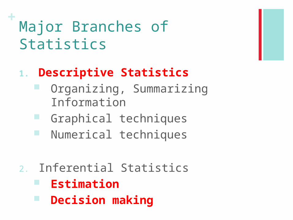
+Major Branches of Statistics

1. Descriptive Statistics Organizing, Summarizing Information Graphical techniques Numerical techniques

2. Inferential Statistics Estimation Decision making

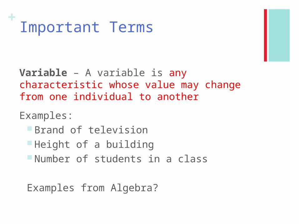
+Important Terms

Variable – A variable is any characteristic whose value may change from one individual to another

Examples: Brand of television Height of a building Number of students in a class

Examples from Algebra?

+Important Terms

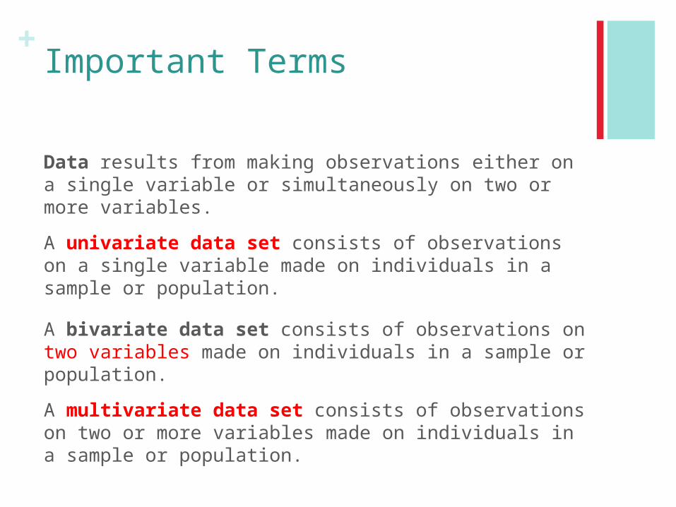
Data results from making observations either on a single variable or simultaneously on two or more variables.

A univariate data set consists of observations on a single variable made on individuals in a sample or population.

A bivariate data set consists of observations on two variables made on individuals in a sample or population.

A multivariate data set consists of observations on two or more variables made on individuals in a sample or population.

+Data Sets

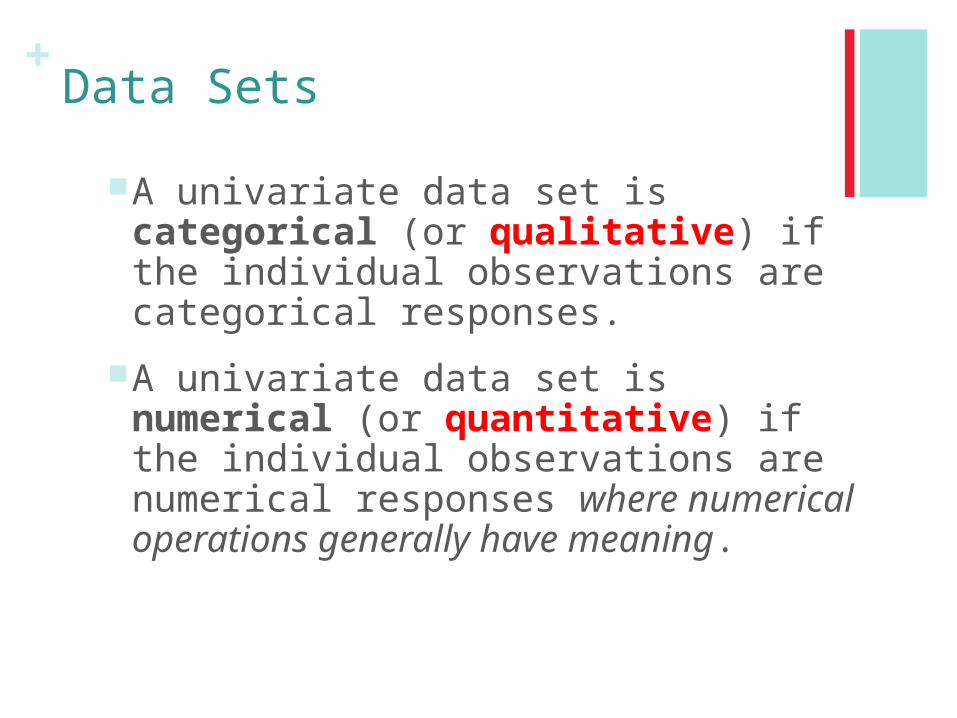
A univariate data set is categorical (or qualitative) if the individual observations are categorical responses.

A univariate data set is numerical (or quantitative) if the individual observations are numerical responses where numerical operations generally have meaning.

+

Categorical Variables place individuals into one of several groups or categories

EXAMPLES?

+Analyzing C

ategorical Data

The distribution of a categorical variable lists the count or percent of individuals who fall into each category.

Frequency Table

Format Count of Stations

Adult Contemporary 1556

Adult Standards 1196

Contemporary Hit 569

Country 2066

News/Talk 2179

Oldies 1060

Religious 2014

Rock 869

Spanish Language 750

Other Formats 1579

Total 13838

Relative Frequency Table

Format Percent of Stations

Adult Contemporary 11.2

Adult Standards 8.6

Contemporary Hit 4.1

Country 14.9

News/Talk 15.7

Oldies 7.7

Religious 14.6

Rock 6.3

Spanish Language 5.4

Other Formats 11.4

Total 99.9

Example, page 8

Count

Percent

Variable

+Analyzing C

ategorical Data

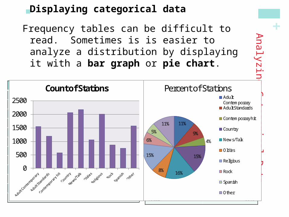
Displaying categorical data

Frequency tables can be difficult to read. Sometimes is is easier to analyze a distribution by displaying it with a bar graph or pie chart.

11%

9%

4%

15%

16%8%

15%

6%

5%

11%

Percent of StationsAdult ContemporaryAdult Standards

Contemporary hit

Country

News/Talk

Oldies

Religious

Rock

Spanish

Other

0

500

1000

1500

2000

2500

Count of StationsFrequency Table

Format Count of Stations

Adult Contemporary 1556

Adult Standards 1196

Contemporary Hit 569

Country 2066

News/Talk 2179

Oldies 1060

Religious 2014

Rock 869

Spanish Language 750

Other Formats 1579

Total 13838

Relative Frequency Table

Format Percent of Stations

Adult Contemporary 11.2

Adult Standards 8.6

Contemporary Hit 4.1

Country 14.9

News/Talk 15.7

Oldies 7.7

Religious 14.6

Rock 6.3

Spanish Language 5.4

Other Formats 11.4

Total 99.9

+Types of Numerical Data

Numerical data is discrete if the possible values are isolated points on the number line.

Numerical data is continuous if the set of possible values form an entire interval on the number line.

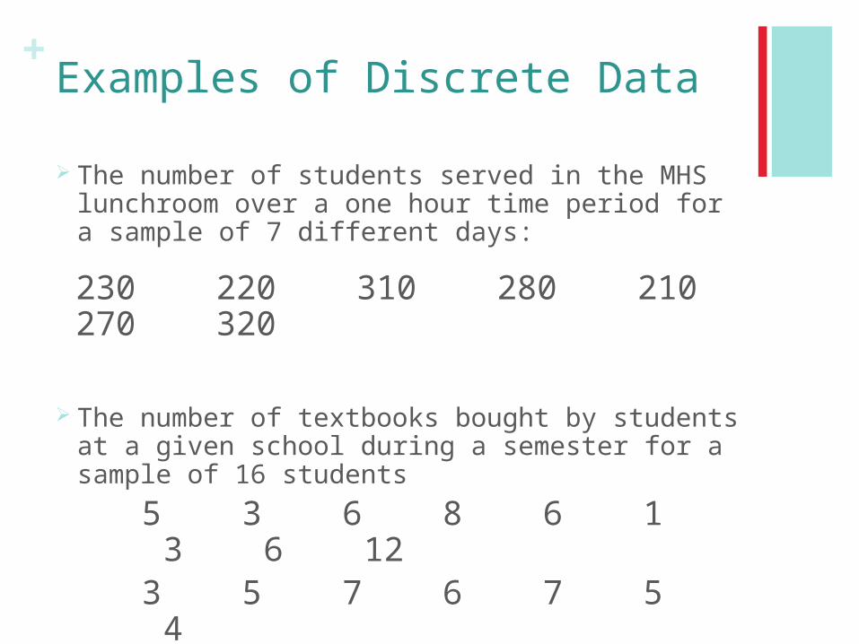
+Examples of Discrete Data

The number of students served in the MHS lunchroom over a one hour time period for a sample of 7 different days:

230 220 310 280 210 270 320

The number of textbooks bought by students at a given school during a semester for a sample of 16 students

5 3 6 8 6 1 3 6 123 5 7 6 7 5 4

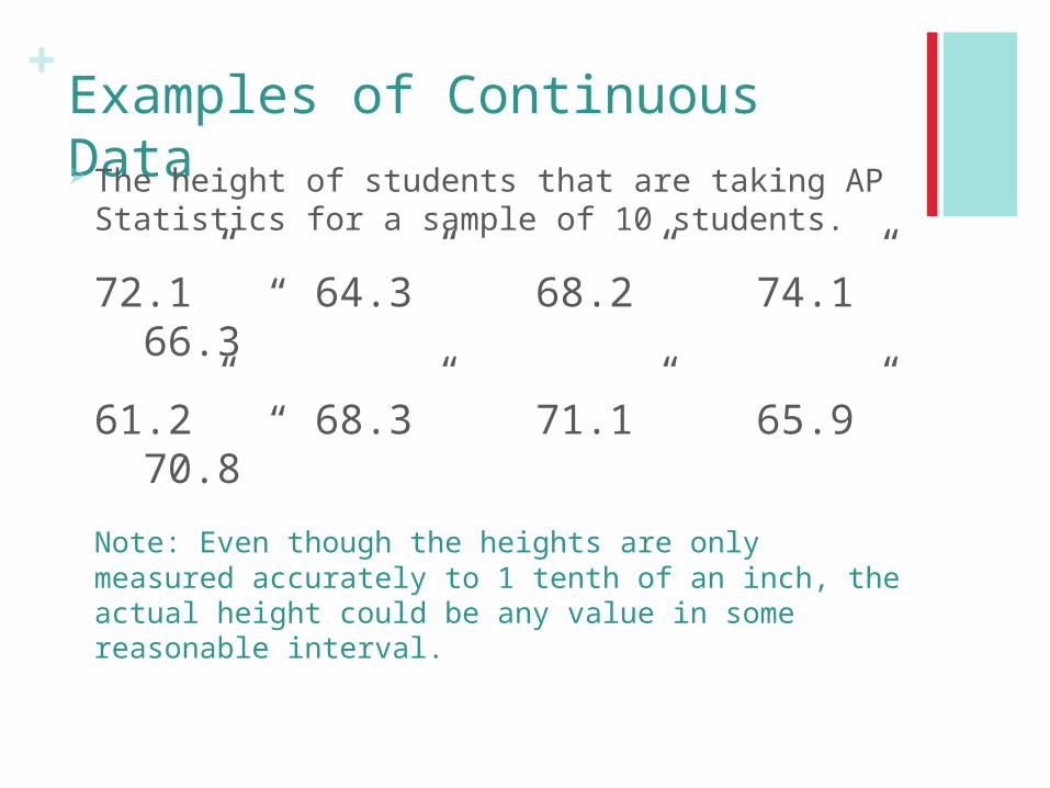
+Examples of Continuous Data The height of students that are taking AP Statistics for a

sample of 10 students.

72.1” 64.3” 68.2” 74.1” 66.3”

61.2” 68.3” 71.1” 65.9” 70.8”

Note: Even though the heights are only measured accurately to 1 tenth of an inch, the actual height could be any value in some reasonable interval.

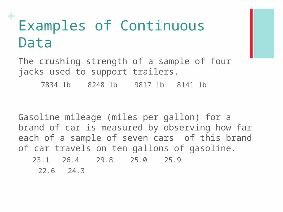
+Examples of Continuous Data

The crushing strength of a sample of four jacks used to support trailers.

7834 lb 8248 lb 9817 lb 8141 lb

Gasoline mileage (miles per gallon) for a brand of car is measured by observing how far each of a sample of seven cars of this brand of car travels on ten gallons of gasoline.

23.1 26.4 29.8 25.0 25.9

22.6 24.3

+

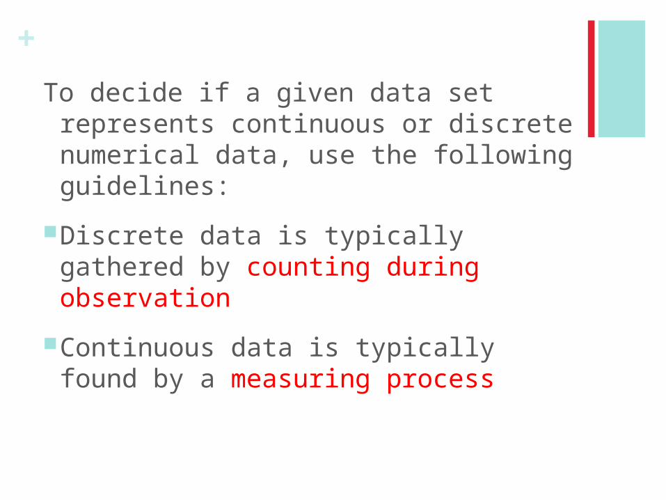
To decide if a given data set represents continuous or discrete numerical data, use the following guidelines:

Discrete data is typically gathered by counting during observation

Continuous data is typically found by a measuring process

+End of Day 1

+Deceptive Graphs

It is important to be an informed consumer by:

• Extracting information from charts and graphs

• Following numerical arguments• Knowing the basics of how data

should be gathered, summarized and analyzed to draw statistical conclusions

• Understanding the validity and appropriateness of processes and decisions that affect your life

+The NY Times ran an article in the “Week in Review” on the housing bubble on 9-23-2007. Included was a graphic that, with some clever scaling, exaggerates the changes in housing prices over the last 20 years.

+Truck B

rands

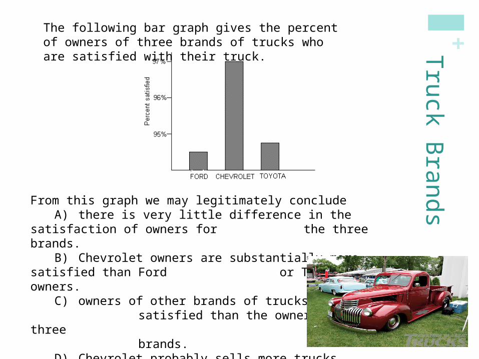
From this graph we may legitimately conclude A) there is very little difference in the satisfaction of

owners for the three brands. B) Chevrolet owners are substantially more satisfied

than Ford or Toyota owners. C) owners of other brands of trucks are less

satisfied than the owners of these three brands.

D) Chevrolet probably sells more trucks than Ford or Toyota.

The following bar graph gives the percent of owners of three brands of trucks who are satisfied with their truck.

+Analyzing C

ategorical Data

Bar graphs compare several quantities by comparing the heights of bars that represent those quantities.

Our eyes react to the area of the bars as well as height. Be sure to make your bars equally wide.

Avoid the temptation to replace the bars with pictures for greater appeal…this can be misleading!

Graphs: Good and Bad

Alternate Example

This ad for DIRECTV has multiple problems. How many can you point out?

+Analyzing C

ategorical Data

Two-Way Tables and Marginal Distributions

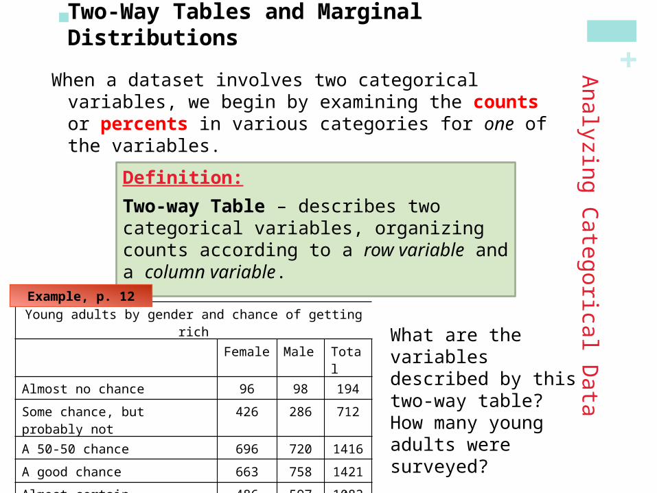
When a dataset involves two categorical variables, we begin by examining the counts or percents in various categories for one of the variables.

Definition:

Two-way Table – describes two categorical variables, organizing counts according to a row variable and a column variable.

Young adults by gender and chance of getting rich

Female Male Total

Almost no chance 96 98 194

Some chance, but probably not 426 286 712

A 50-50 chance 696 720 1416

A good chance 663 758 1421

Almost certain 486 597 1083

Total 2367 2459 4826

Example, p. 12

What are the variables described by this two-way table?How many young adults were surveyed?

+Analyzing C

ategorical Data

Two-Way Tables and Marginal Distributions

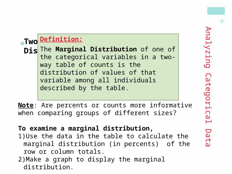
Definition:

The Marginal Distribution of one of the categorical variables in a two-way table of counts is the distribution of values of that variable among all individuals described by the table.

Note: Are percents or counts more informative when comparing groups of different sizes?

To examine a marginal distribution,1)Use the data in the table to calculate the marginal

distribution (in percents) of the row or column totals.2)Make a graph to display the marginal distribution.

+

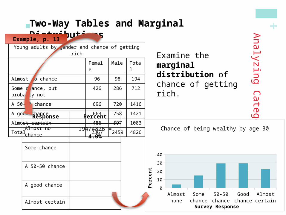
Young adults by gender and chance of getting rich

Female Male Total

Almost no chance 96 98 194

Some chance, but probably not 426 286 712

A 50-50 chance 696 720 1416

A good chance 663 758 1421

Almost certain 486 597 1083

Total 2367 2459 4826

Analyzing C

ategorical Data

Two-Way Tables and Marginal Distributions

Response Percent

Almost no chance 194/4826 = 4.0%

Some chance

A 50-50 chance

A good chance

Almost certain

Example, p. 13

Examine the marginal distribution of chance of getting rich.

Almost none

Some chance

50-50 chance

Good chance

Almost certain

05

101520253035

Chance of being wealthy by age 30

Survey Response

Perc

ent

+Analyzing C

ategorical Data

Relationships between Categorical Variables Marginal distributions tell us nothing about the relationship

between two variables.

Definition:

A Conditional Distribution of a variable describes the values of that variable among individuals who have a specific value of another variable.

To examine or compare conditional distributions,1)Select the row(s) or column(s) of interest.2)Use the data in the table to calculate the conditional

distribution (in percents) of the row(s) or column(s).3)Make a graph to display the conditional distribution.

• Use a side-by-side bar graph or segmented bar graph to compare distributions.

+

Young adults by gender and chance of getting rich

Female Male Total

Almost no chance 96 98 194

Some chance, but probably not 426 286 712

A 50-50 chance 696 720 1416

A good chance 663 758 1421

Almost certain 486 597 1083

Total 2367 2459 4826

Analyzing C

ategorical Data

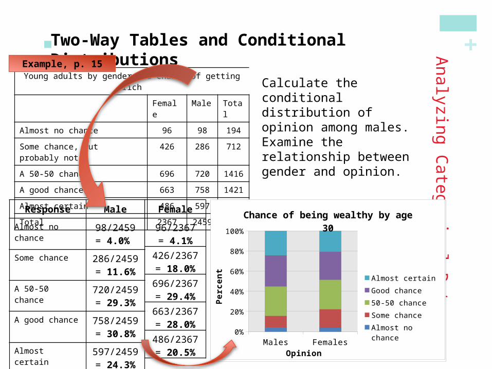
Two-Way Tables and Conditional Distributions

Response Male

Almost no chance 98/2459 = 4.0%

Some chance 286/2459 = 11.6%

A 50-50 chance 720/2459 = 29.3%

A good chance 758/2459 = 30.8%

Almost certain 597/2459 = 24.3%

Example, p. 15

Calculate the conditional distribution of opinion among males.Examine the relationship between gender and opinion.

Almost no chance

Some chance

50-50 chance

Good chance

Almost certain

0

10

20

30

40

Chance of being wealthy by age 30

Males

Series2

Opinion

Perc

ent

Female

96/2367 = 4.1%

426/2367 = 18.0%

696/2367 = 29.4%

663/2367 = 28.0%

486/2367 = 20.5%

Almost no

chance

Some chance

50-50 chance

Good chance

Almost certain

0

10

20

30

40

Chance of being wealthy by age 30

Males

Females

Opinion

Perc

ent

Males Females0%

10%20%30%40%50%60%70%80%90%

100%

Chance of being wealthy by age 30

Almost certain

Good chance

50-50 chance

Some chance

Almost no chance

Opinion

Perc

ent

+Analyzing C

ategorical Data

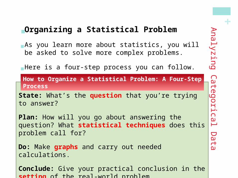
Organizing a Statistical Problem As you learn more about statistics, you will be asked to solve

more complex problems.

Here is a four-step process you can follow.

State: What’s the question that you’re trying to answer?

Plan: How will you go about answering the question? What statistical techniques does this problem call for?

Do: Make graphs and carry out needed calculations.

Conclude: Give your practical conclusion in the setting of the real-world problem.

How to Organize a Statistical Problem: A Four-Step Process