lecture notes 3tu course applied statistics

12

Lecture Notes

3TU Course Applied Statistics

A. Di Bucchianico

14th May 2008

A. Di Bucchianico 14th May 2008 ii

Contents

Preface 1

1 Short Historical Introduction to SPC 31.1 Goal of SPC . . . . . . . . . . . . . . . . . . . . . . . . . . . . . . . . . . . . . . 31.2 Brief history of SPC . . . . . . . . . . . . . . . . . . . . . . . . . . . . . . . . . 41.3 Statistical tools in SPC . . . . . . . . . . . . . . . . . . . . . . . . . . . . . . . 51.4 Exercises . . . . . . . . . . . . . . . . . . . . . . . . . . . . . . . . . . . . . . . . 6

2 A Short Introduction to R 72.1 The R initiative . . . . . . . . . . . . . . . . . . . . . . . . . . . . . . . . . . . . 72.2 R basics . . . . . . . . . . . . . . . . . . . . . . . . . . . . . . . . . . . . . . . . 8

2.2.1 Data files . . . . . . . . . . . . . . . . . . . . . . . . . . . . . . . . . . . 82.2.2 Probability distributions in R. . . . . . . . . . . . . . . . . . . . . . . . . 82.2.3 Graphics in R . . . . . . . . . . . . . . . . . . . . . . . . . . . . . . . . . 92.2.4 Libraries in R . . . . . . . . . . . . . . . . . . . . . . . . . . . . . . . . . 92.2.5 Basic statistics in R . . . . . . . . . . . . . . . . . . . . . . . . . . . . . . 102.2.6 Functions in R . . . . . . . . . . . . . . . . . . . . . . . . . . . . . . . . . 102.2.7 Editors for R . . . . . . . . . . . . . . . . . . . . . . . . . . . . . . . . . 10

2.3 Exercises . . . . . . . . . . . . . . . . . . . . . . . . . . . . . . . . . . . . . . . . 10

3 Process Capability Analysis 133.1 Example of a process capability analysis . . . . . . . . . . . . . . . . . . . . . . 133.2 Basic properties of capability indices . . . . . . . . . . . . . . . . . . . . . . . . 163.3 Parametric estimation of capability indices . . . . . . . . . . . . . . . . . . . . 183.4 Exact distribution of capability indices . . . . . . . . . . . . . . . . . . . . . . . 233.5 Asymptotic distribution of capability indices . . . . . . . . . . . . . . . . . . . . 243.6 Tolerance intervals . . . . . . . . . . . . . . . . . . . . . . . . . . . . . . . . . . 273.7 Normality testing . . . . . . . . . . . . . . . . . . . . . . . . . . . . . . . . . . . 313.8 Mathematical background on density estimators . . . . . . . . . . . . . . . . . . 34

3.8.1 Finite sample behaviour of density estimators . . . . . . . . . . . . . . . 343.8.2 Asymptotic behaviour of kernel density estimators . . . . . . . . . . . . 36

3.9 Exercises . . . . . . . . . . . . . . . . . . . . . . . . . . . . . . . . . . . . . . . . 40

4 Control Charts 434.1 The Shewhart X chart . . . . . . . . . . . . . . . . . . . . . . . . . . . . . . . . 44

4.1.1 Additional stopping rules for the X control chart . . . . . . . . . . . . . 454.2 Shewhart charts for the variance . . . . . . . . . . . . . . . . . . . . . . . . . . 45

iii

CONTENTS

4.2.1 The mean and variance of the standard deviation and the range . . . . . 464.2.2 The R control chart . . . . . . . . . . . . . . . . . . . . . . . . . . . . . 474.2.3 The S and S2 control charts . . . . . . . . . . . . . . . . . . . . . . . . . 48

4.3 Calculation of run lengths for Shewhart charts . . . . . . . . . . . . . . . . . . . 494.4 CUSUM procedures . . . . . . . . . . . . . . . . . . . . . . . . . . . . . . . . . 534.5 EWMA control charts . . . . . . . . . . . . . . . . . . . . . . . . . . . . . . . . 574.6 Exercises . . . . . . . . . . . . . . . . . . . . . . . . . . . . . . . . . . . . . . . . 57

5 Solutions Exercises Historical Introduction to SPC 61

6 Solutions Exercises Introduction to R 65

7 Solutions Exercises Process Capability Analysis 67

8 Solutions Exercises Control Charts 75

Appendix A: Useful Results from Probability Theory 79

Index 83

References 86

A. Di Bucchianico 14th May 2008 iv

List of Figures

1.1 Some famous names in SPC. . . . . . . . . . . . . . . . . . . . . . . . . . . . . . 4

3.1 Two histograms of the same sample of size 50 from a mixture of 2 normaldistributions. . . . . . . . . . . . . . . . . . . . . . . . . . . . . . . . . . . . . . 32

4.1 Shewhart X-chart with control lines. . . . . . . . . . . . . . . . . . . . . . . . . 44

v

LIST OF FIGURES

A. Di Bucchianico 14th May 2008 vi

List of Tables

2.1 Names of probability distributions in R. . . . . . . . . . . . . . . . . . . . . . . 92.2 Names of probability functions in R. . . . . . . . . . . . . . . . . . . . . . . . . 92.3 Names of goodness-of-fit tests in R. . . . . . . . . . . . . . . . . . . . . . . . . . 9

3.1 Well-known kernels for density estimators. . . . . . . . . . . . . . . . . . . . . . 33

4.1 Control chart constants. . . . . . . . . . . . . . . . . . . . . . . . . . . . . . . . 48

vii

LIST OF TABLES

A. Di Bucchianico 14th May 2008 viii

Preface

These notes are the lecture notes for the Applied Statistics course. This course is an electivecourse in the joint Master’s programme of the three Dutch technical universities and is alsopart of the Dutch National Mathematics Master’s Programme. The course Applied Statisticshas an alternating theme. In the even years the theme is Statistical Process Control, while inthe odd years the theme is Survival Analysis.

Statistical Process Control (SPC) is a name to describe a set of statistical tools that havebeen widely used in industry since the 1950’s and lately also in business (in particular, infinancial and health care organisations). Students taking a degree in statistics or appliedmathematics should therefore be acquainted with the basics of SPC.

Modern applied statistics is unthinkable without software. In my opinion, statisticiansshould be able to perform both quick analyses using a graphical (Windows) interface and beable to write scripts for custom analyses. For this course, we use the open source statisticalsoftware R, which is available from www.r-project.org. Please note that R-scripts are verysimilar to scripts in S and S-Plus. Use of other standard software will be demonstrated duringthe lecture notes, but is not included in these lecture notes. We try to achieve with this coursethat students

• learn the basics of practical aspects SPC

• learn the mathematical background of the basic procedures in SPC

• learn to discover the drawbacks of standard practices in SPC

• learn to perform analyses and simulations using R.

General information on this course will be made available through the web site

www.win.tue.nl/ ∼ adibucch/2WS10.

My personal motivation for writing these lecture notes is that I am unaware of a suitabletext book on SPC aimed at students with a background in mathematical statistics. Mosttext books on SPC aim at an audience with limited mathematical background. Exceptionsare Kenett and Zacks (1998) and Montgomery (2000) which are both excellent books (theformer addresses much more advanced statistical techniques than the latter), but they do notsupply enough mathematical background for the present course. Kotz and Johnson (1993)supplies enough mathematical background, but deals with capability analysis only. Czitromand Spagon (1997) is a nice collection of challenging case studies in SPC that cannot be solvedwith standard methods.

1

Finally, I would like to gratefully acknowledge the extensive help of my student assistantXiaoting Yu for helping me in making solutions to exercises, R procedures and preparing datasets.

Eindhoven, January 31, 2008Alessandro Di Bucchianico

www.win.tue.nl/∼adibucch

A. Di Bucchianico 14th May 2008 2 of 91

Chapter 1

Short Historical Introduction to SPC

Contents

1.1 Goal of SPC . . . . . . . . . . . . . . . . . . . . . . . . . . . . . . . 3

1.2 Brief history of SPC . . . . . . . . . . . . . . . . . . . . . . . . . . . 4

1.3 Statistical tools in SPC . . . . . . . . . . . . . . . . . . . . . . . . . 5

1.4 Exercises . . . . . . . . . . . . . . . . . . . . . . . . . . . . . . . . . . 6

Statistical Process Control (SPC) is a name to describe a set of statistical tools that havebeen widely used in industry since the 1950’s and in business (in particular, in financial andhealth care organisations) since the 1990’s. It is an important part of quality improvementprogrammes in industry. A typical traditional setting for SPC is a production line in a factory.Measurements of important quality characteristics are being taken at fixed time points. Thesemeasurements are being used to monitor the production process and to take appropriate actionwhen the process is not functioning well. In such cases we speak of an out-of-control situation.

In this chapter we will give a brief overview of the goals and history of SPC, as well asdescribe the statistical machinery behind SPC.

1.1 Goal of SPC

The ultimate goal of SPC is to monitor variation in production processes. There is a widelyused (but somewhat vaguely defined) terminology to describe the variation in processes. Fol-lowing the terminology of Shewhart, variation in a production process can have two possiblecauses:

• common causes

• special causes

Common causes refer to natural, inherent variation that cannot be reduced without makingchanges to the process such as improving equipment or using other machines. Such variationis often considered to be harmless or it may unfeasible for economical or technical reasons toreduce it. Special causes refer to variation caused by external causes such as a broken part of

3

1.2. BRIEF HISTORY OF SPC

a machine. Such causes lead to extra unnecessary variation and must therefore be detectedand taken away as soon as possible.

A process that is only subject to common causes is said to be in-control. To be a little bitmore precise, an in-control process is a process that

• only has natural random fluctuations (common causes)

• is stable

• is predictable.

An process that is not in-control is said to be out-of-control. An important practical impli-cation is that one should avoid making changes to processes that are not in-control, becausesuch changes may not be lasting.

1.2 Brief history of SPC

Deming Shewhart Box

Taguchi Juran Ishikawa

Figure 1.1: Some famous names in SPC.

Shewhart is usually considered to be the founding father of SPC. As starting point one usuallyconsiders the publication of an internal Bell Labs report in 1924. In this note Shewhartdescribed the basic form of what is now called the Shewhart X control chart. His subsequentideas did not catch on with other American companies. One of the few exceptions was WesternElectric, where Deming and Juran worked. The famous Western Electric Company 1956handbook still makes good reading. The breakthrough for SPC techniques came after World


1.3. STATISTICAL TOOLS IN SPC

War II when Deming (a former assistant to Shewhart) was hired by the Japanese government toassist in rebuilding the Japanese industry. The enormous successes of the Japanese industry inthe second half of the 20th century owes much to the systematic application of SPC, which wasadvocated with great enthusiasm by Ishikawa. In the early 1950’s Box introduced experimentaldesign techniques developed by Fisher and Yates in an agricultural context, in industry, inparticular in chemical industries. He made extensive contributions to experimental designsfor optimization. Later he moved to the United States and successfully started and led theCenter for Quality and Productivity Improvement at the University of Wisconsin-Madison.Experimental design was developed in a different way by Taguchi, who successfully introducedit to engineers. It was not until the 1980’s that American companies after severe financiallosses began thinking of introducing SPC. Motorola became famous by starting the Six Sigmaapproach, a quality improvement programme that heavily relies on statistics. Both the Taguchiand the Six Sigma approach are being used world-wide on a large scale. The developmentsin Europe are lagging behind. An important European initiative is ENBIS, the EuropeanNetwork for Business and Industrial Statistics (www.enbis.org. This initiative by Bisgaard, aformer successor of Box at the University of Wisconsin-Madison, successfully brings togetherstatistical practitioners and trained statisticians from industry and academia.

1.3 Statistical tools in SPC

Since users of SPC often do not have a background in statistics, there is a strong tendency touse simple statistical tools, sometimes denoted by fancy names like “The Magnificent Seven”.In many cases this leads to unnecessary oversimplifications and poor statistical analyses. It iscurious that several practises like the use of the range instead of the standard deviation arestill being advocated, although the original reason (ease of calculation) has long ceased to berelevant. For more information on this topic we refer to Stoumbos et al. (2000), Woodall andMontgomery (1999) and Woodall (2000).

As with all statistical analyses, graphical methods are important and should be used fora first inspection. Scatterplots and histograms are often used. Another simple tool is thePareto chart. This chart (introduced by Juran) is simple bar chart that shows in an orderedway the most important causes for errors or excessive variation. The rationale is the so-called 80 − 20 rule (often attributed to the econometrician Pareto), which says that 80%of damage comes from 20% of causes. Histograms are still being used to assess normalityof data, although it is widely known that the choice of bins heavily influences the shape ofthe histogram (see Section 3.8). The use of quantile plots like the normal probability plotor density estimators like kernel density estimators is not widespread (for an exception, seeRodriguez (1992)). In SPC it is often useful to obtain accurate estimate of tail probabilitiesand quantiles. A typical example are the so-called capability analyses, where process variationis compared with specifications in order to judge whether a production process is capable ofmeeting specifications (see Chapter 3). This judgement is often based on so-called capabilityindices, which are often simple parametric estimators of tail probabilities that may not bereliable in practice. Alternatives are tolerance intervals (both parametric and distribution-free; see Section 3.6) that are interval estimators containing a specified part of a distributionor tail estimators based on extreme value theory (although these often require sample sizesthat are not available in industrial practice).

Control charts are the most widely known tools in SPC. They are loosely speaking a graph-


1.4. EXERCISES

ical way to perform repeated hypothesis testing. Shewhart control charts can be interpreted assimple sequential likelihood ration tests depending on the current statistics (a individual ob-servation or a group mean or standard deviation) only, while the Cumulative Sum (CUSUM)charts introduced by Page in the 1950’s can be seen as sequential generalized likelihood ratiotests based on all data. These charts also appear change point analysis. The ExponentiallyWeighted Moving Average (EWMA) charts introduced in Girshick and Rubin (1952), Roberts(1959) and Shiryaev (1963) were inspired by Bayesian statistics, but the procedures have atime series flavour.

In this course we will concentrate on univariate SPC. However, in industrial practiceoften several quality characteristics are needed to accurately monitor a production processes.These characteristics are often correlated. Hence, techniques from multivariate statistics likeprincipal components are required. For a readable overview of this aspect, we refer to Qin(2003).

General papers with more information about developments of statistical techniques forSPC include Crowder et al. (1997), Hawkins et al. (2003), Lai (1995), Lai (2001), and Palmet al. (1997).

1.4 Exercises

Read the paper Provost and Norman (1990) and answer the following questions.

Exercise 1.1 Describe the three methods of managing variation mentioned in the text.

Exercise 1.2 Describe the different test methods mentioned in this text.

Exercise 1.3 Why was variation not a critical issue in the period before 1700?

Exercise 1.4 When and why did variation become a critical issue?

Exercise 1.5 What was the reason that standards for inspection were formulated at the endof the 19th century?

Exercise 1.6 Explain the go/no-go principle.

Exercise 1.7 What is the goal of setting tolerances and specifications?

Exercise 1.8 Explain the term interchangeability and give an example of a “modern” productwith interchangeable components

Exercise 1.9 Explain the relation between interchangeable components and variation.

Exercise 1.10 What is the goal of a Shewhart control chart?

Exercise 1.11 In what sense does Shewhart’s approach differ from the approach based onsetting specifications?

Exercise 1.12 What were the reasons for Shewhart to put control limits at a distance of3 standard deviations of the target value?

Exercise 1.13 Explain the idea behind Taguchi’s quadratic loss function.

Exercise 1.14 Explain what is meant by tolerance stack-up (see p. 44, 1st paragraph belowFigure 3).


Chapter 2

A Short Introduction to R

Contents

2.1 The R initiative . . . . . . . . . . . . . . . . . . . . . . . . . . . . . 7

2.2 R basics . . . . . . . . . . . . . . . . . . . . . . . . . . . . . . . . . . 8

2.2.1 Data files . . . . . . . . . . . . . . . . . . . . . . . . . . . . . . . . . 8

2.2.2 Probability distributions in R. . . . . . . . . . . . . . . . . . . . . . . 8

2.2.3 Graphics in R . . . . . . . . . . . . . . . . . . . . . . . . . . . . . . . 9

2.2.4 Libraries in R . . . . . . . . . . . . . . . . . . . . . . . . . . . . . . . 9

2.2.5 Basic statistics in R . . . . . . . . . . . . . . . . . . . . . . . . . . . . 10

2.2.6 Functions in R . . . . . . . . . . . . . . . . . . . . . . . . . . . . . . 10

2.2.7 Editors for R . . . . . . . . . . . . . . . . . . . . . . . . . . . . . . . 10

2.3 Exercises . . . . . . . . . . . . . . . . . . . . . . . . . . . . . . . . . . 10

2.1 The R initiative

There are many commercial statistical softwares available. Well-known examples include SAS,SPSS, S-Plus, Minitab, Statgraphics, GLIM, and Genstat. Usually there is a GUI (graphicaluser interface). Some softwares allow to perform analyses using the GUI as well as by typingcommands on a command line. Larger analyses may be performed by executing scripts.

In the 1970’s Chambers of AT&T started to develop a computer language (called S) thatwould be able to perform well-structured analyses. A commercial version of S appearedin the early 1990’s under the name S-Plus. Ihaka and Gentleman developed a little bitlater a free, open source language R which is very similar to S. Currently R is being main-tained and continuously improved by a group of world class experts in computational statis-tics. Hence, R has gained enormous popularity among various groups of statisticians, includ-ing mathematical statisticians and biostatisticians. The R-project has its own web page atwww.r-project.org. Downloads are available through the CRAN (Comprehensive R ArchiveNetwork) at www.cran.r-project.org.

7

2.2. R BASICS

2.2 R basics

There are several tutorials available inside R through Help or can be found on the web, e.g.through CRAN. The R reference card is very useful. Within R further help can be obtainedby typing help when one knows the name of a function (e.g., help(pnorm)) or help.searchwhen one only keywords (e.g., help.search(“normal distribution”)).

2.2.1 Data files

Assignment are read from right to left using the ← operator:

a < −2 + sqrt(5)

There are several form of data objects. Vectors can be formed using the c operator (concate-nation), e.g.,

a < −c(1, 2, 3, 10)yields a vector consisting of 4 numbers. Vectors may be partitioned into matrices by usingthe matrix command, e.g.,

matrix(c(1, 2, 3, 4, 5, 6), 2, 3, byrow = T)

creates a matrix with 2 rows and 3 columns.The working directory may be set by setwd and displayed by getwd() (this will return an

empty answer if no working directory has been set). Please note that directory names shouldbe written with quotes and that the Unix notation must be used even if R is being used underWindows, e.g. setwd(“F:/2WS10”). A data set may be turned into the default data set byusing the command attach; the companion command detach. Data files on a local file systemmay be read through the command scan when there is only one column or otherwise by

read.table(“file.txt′′, header = TRUE)

Both read.table and scan can read data files from the WWW (do not forget to put quotesaround the complete URL).

Parts of data files may be extracted by using so-called subscripting. The command d[r,]

yields the rth row of object d, while d[, c] yields the cth column of object d. The entry in rowr and column c of object d can be retrieved by using d[r,c]. Extracting elements that satisfya certain condition may also be extracted by subscripting. E.g., d[d<20] yields all elementsof d that do not exceed 20, while d[“age”] extracts the column with name “age” (note thedouble quotes) from object d. The number of elements of an object d is given by length(d).

2.2.2 Probability distributions in R.

Standard probability distributions have short names in R as given by Table 2.1. Severalprobability functions are available. Their names consists of two parts: the first part is thename of the function (see Table 2.2), while the second part is the name as in Table 2.1.E.g., a sample of size 10 from an exponential distribution with mean 3 is generated in R byrexp(10,1/3) (R uses the failure intensity instead of the mean as parameter).Table 2.3 lists several goodness-of-fit tests that are available in R, either directly or via thepackage nortest (see Subsection 2.2.4).


2.2. R BASICS

Distribution Name in R

normal norm

(non-central) Student T t

Weibull weibull

exponential exp

(non-central) χ2 chisq

Gamma gamma

F f

Table 2.1: Names of probability distributions in R.

Function Name in R

d densityp probability = cumulative distribution functionq quantiler random numbers

Table 2.2: Names of probability functions in R.

2.2.3 Graphics in R

The standard procedure in R to make 1D and 2D plots is plot. Histogram are availablethrough hist. These commands can be supplied with options to allow for titles, subtitles,and labels on the x-axes:

plot(data,main=‘‘Title’’,sub=‘‘Subtitle’’,xlab=‘‘X-axis’’,ylab=‘‘Y-axis’’)

Quantile-quantile plots are available through qqplot, while qqnorm yields a plot of the quan-tiles of a data set against the quantiles of a fitted normal distribution (normal probability plot).A Box-and-Whisker plot is also available for exploratory data analysis through boxplot (ifthe data set is a data frame like produced by read.table, then multiple Box-and-Whiskerplots are produced). The empirical cumulative distribution function is available through ecdf.Kernel density estimators are available through density. Graphics can be saved to files bychoosing File and Save as in the menu of the R console.

2.2.4 Libraries in R

Extensions to the basic functions are available through libraries of functions. In the Windowsinterface of R, these libraries can be loaded or installed by choosing the option Packages in

Test Name in R Package

Shapiro-Wilks shapiro.test statsKolmogorov (1-sample) ks.test stats

Smirnov (2-sample) ks.test statsAnderson-Darling ad.test nortest

Cramér-von Mises test cvm.test nortestLilliefors test lillie.test nortest

Table 2.3: Names of goodness-of-fit tests in R.


2.3. EXERCISES

the menu. Libraries may also contain ways to improve exchange of files with other softwarelike Matlab or WinEdt. Examples of useful libraries include:

survival: library for survival analysis (Cox proportional hazards etc.)

qcc: SPC library

RWinEdt: interface with editor WinEdt (recommended for testing scripts, see also Subsec-tion 2.2.7)

RMatlab: a bidirectional interface with Matlab

2.2.5 Basic statistics in R

Summary statistics of a data set can be obtained from summary, or by using individual com-mands like mean, sd, mad, and IQR. Standard hypothesis tests are also available, e.g., t.testyields the standard tests for means of one or two normal samples.

2.2.6 Functions in R

Analyses that have to be performed often can be put in the form of functions, e.g..,

simple < − function(data, mean = 0, alpha = 0.05)

{hist(data), t.test(data, conf.level = alpha, mu = mean)}

This means that typing simple(data,4) uses the default value α = 0.05 and tests the nullhypothesis µ = 4.

2.2.7 Editors for R

Instead of pasting commands from an ordinary text editor into the R console, one may alsouse WinEdt as R editor by using the RWinEdt package. Another choice is Tinn-R, which isa free R editor that helps the user by showing R syntaxis while typing.

2.3 Exercises

Exercise 2.1 Calculate in R the probability that a random variable with a χ2 distribution with3 degrees of freedom is larger than 5.2.

Exercise 2.2 Compute the 0.99 quantile of the standard normal distribution.

Exercise 2.3 Generate 20 random numbers from an exponential distribution with mean 3.How can you check that you choose the right parametrization?

Exercise 2.4 Generate 40 random numbers from a normal distribution with mean 10 andvariance 2. Make a histogram and play with the number of bins to convince yourself of theinfluence on the shape. Check normality through a normal probability plot, a plot of the densityand an appropriate goodness-of-fit test. Also test the mean and variance of the sample.


2.3. EXERCISES

Exercise 2.5 A telecommunication company has entered the market for mobile phones in anew country. The company’s marketing manager conducts a survey of 200 new subscribersfor mobile phones. The data of her survey are in the data set telephone.txt, which containsthe first month’s bills. Make an appropriate plot of this data set. What information can beextracted from these data? What marketing advice would you give to the marketing manager?

Exercise 2.6 Dried eggs are being sold in cans. Each can contains two different types ofeggs. As part of a quality control programme, the fat content of eggs is being investigated. Theinvestigation is divided over 6 different laboratories. Every laboratory receives the same numberof eggs of both types. Testing the fat content of eggs is destructive, so that each egg can onlybe investigated once. Since measuring the fat content is time consuming, the measurementsare divided over 2 laboratory assistants within each laboratory.

A quality manager applies a certain statistical procedure and claims that there is a sig-nificant difference between the fat contents measured by the laboratories. This report causesconfusion, since the 6 laboratories all have a good reputation and there is no reason to expectlarge variation in fat content of the eggs. Find an explanation by making appropriate plots ofthe data set eggs.txt.

Exercise 2.7 Supermarket chain ATOHIGH has two shops A and B in a certain town. Bothstores are similar with respect to size, lay-out, number of customers and spending per customer.The populations of the parts of town of the two shops are quite similar. Management decidesto experiment with the lay-out of shop A, including different lighting. After some time asurvey is performed on a Saturday afternoon among 100 customers in both shops. The surveyis restricted to customers which are part of a family of at least 3 persons. The data setsupermarket.txt contains the data of this survey. Perform a statistical analysis of this dataset, both by producing appropriate plots and by computing appropriate summary statistics.What can you conclude about the spending in both shops?

Exercise 2.8 Write an R function that computes the empirical survivor function given a dataset. The empirical survivor function at a point x counts the proportion of observations exceed-ing x.

Exercise 2.9 Write an R function that produces a confidence interval for the variance from asample from the normal distribution.

Exercise 2.10 Write a function that plots a plot of the values of a data set against the quan-tiles of a given Weibull distribution. Test your function with a

1. a random sample of size 30 from a Weibull distribution with shape parameter 3 and scaleparameter 2.

2. a random sample of size 30 from a Gamma distribution with shape parameter 7.57 andrate parameter 0.235. Check using formulas that the mean and variance of this Gammadistribution is approximately equal to the mean and variance of the Weibull distributionin 1).

Exercise 2.11 In the 19th century French physicists Fizeau and Foucault independently in-vented ways to measure the speed of light. Foucault’s method turned out to be the most accurate


2.3. EXERCISES

one. The Foucault method is based on fast rotation mirrors. The American physicists Michel-son and Newcomb improved Foucault’s method. The data set light.txt contains measure-ments by Newcomb from 1882. The data are coded times needed by light to travel a distance of3721 metres across a river and back. The coding of these measurements was as follows: fromthe original times in microseconds measured by Newcomb first 24.8 was subtracted, after whichthe results were multiplied with 1000.

1. Compute a 95% confidence interval for the average speed of light.

2. State the assumptions on which the above interval is based. Check your assumptions witha suitable plot. What is your conclusion?

3. Make a box plot of the data. What do you observe?

4. Plot the data against the observation number. Provide a possible explanation for whatyou observed in part c).

5. Recompute a 95% confidence interval for the average speed of light using your findingsof part c).

6. Use the WWW to find the currently most accurate value for the speed of light. Testwhether this new value is consistent with the measurements of Newcomb.

Exercise 2.12 To improve rain fall in dry areas, an experiment was carried out with 52clouds. Scientists investigated whether the addition of silver nitrate has a positive effect onrainfall. They chose 26 out of a sample of 52 clouds and seeded it with silver nitrate. Theremaining 26 clouds were not treated with silver nitrate. The data set clouds.txt records therainfall in feet per acre.

1. Apply a t-test to investigate whether the average rainfall increased by adding silver ni-trate. Argue whether the data are paired or not.

2. The t-test assumes normally distributed data. Check both graphically and by using aformal test whether the data are normally distributed. What conclusion should you drawon the test performed in part a)?

3. Because the scientists thought that addition of silver nitrate should have a multiplicativeeffect, they suggested transforming the data. What transformation should be a logicalcandidate? What effect does this transformation have on the normality assumption?Apply the t-test of part a) on the transformed data. What is your final conclusion onthe addition of silver nitrate?


Chapter 3

Process Capability Analysis

Contents

3.1 Example of a process capability analysis . . . . . . . . . . . . . . 13

3.2 Basic properties of capability indices . . . . . . . . . . . . . . . . . 16

3.3 Parametric estimation of capability indices . . . . . . . . . . . . 18

3.4 Exact distribution of capability indices . . . . . . . . . . . . . . . 23

3.5 Asymptotic distribution of capability indices . . . . . . . . . . . . 24

3.6 Tolerance intervals . . . . . . . . . . . . . . . . . . . . . . . . . . . . 27

3.7 Normality testing . . . . . . . . . . . . . . . . . . . . . . . . . . . . 31

3.8 Mathematical background on density estimators . . . . . . . . . 34

3.8.1 Finite sample behaviour of density estimators . . . . . . . . . . . . . 34

3.8.2 Asymptotic behaviour of kernel density estimators . . . . . . . . . . 36

3.9 Exercises . . . . . . . . . . . . . . . . . . . . . . . . . . . . . . . . . . 40

In this chapter we present the mathematical background of process capability analysis. Wefocus in particular on the distributional properties of the capability indices Cp and Cpk andrelated topics like tolerance intervals and density estimation. We refer to Kotz and Johnson(1993) for further information on the mathematical background of capability indices and toKotz and Lovelace (1998) for further information on applications of capability indices.

3.1 Example of a process capability analysis

In this section we first present the basic ideas behind process capability analyses and thenillustrate these ideas with a small case study. In particular, we show how to perform theanalysis using the qcc package for R.

Usually the items produced by a production process have to meet customer requirements.Requirements may also be set by the government through legislation. It is therefore importantto know beforehand whether the inherent variation within the production process is such thatit can meet these requirements. Requirements are usually defined as specification limits.We denote the upper specification limit by USL and the lower specification limit by LSL.Products that fall outside specification limits are called non-conforming. Within SPC an

13

3.1. EXAMPLE OF A PROCESS CAPABILITY ANALYSIS

investigation whether the process can meet the requirements is called a Process CapabilityAnalysis. Basically one wishes to determine 1 − P (LSL < X < USL), the probability ofa non-conforming item where X denotes the essential quality characteristic (of course, inpractice one usually has more than one important quality characteristic). Such a capabilityanalysis is usually performed at the end of the so-called Phase I of a production process, e.g.,the phase in which a pilot study is performed in order to decide whether it is possible to startfull production.

A straightforward way to describe process capability would be to use the sample meanand sample standard deviation. As natural bandwidth of a process one usually takes 6σ,which implicitly assumes a normal distribution. For a random variable X which is normallydistributed X with parameters µ and σ2, it holds that P (X > µ + 3σ) = 0.00135, and thusP (µ− 3σ < X < µ + 3σ) = 0.9973. This is a fairly arbitrary, but widely accepted choice.

Whether a process fits within the 6σ-bandwidth, is often indicated in industry by so-calledProcess Capability Indices. Several major companies request from their suppliers detaileddocumentation proving that the production processes of the supplier has certain minimalvalues for the process capability indices Cp and Cpk defined below. These minimal values usedto be 1.33 or 1.67, but increasing demands on quality often requires values larger than 2. Thesimplest capability index is called Cp (in order to avoid confusion with Mallow’s regressiondiagnostic value Cp one sometimes uses Pp) and is defined as

Cp =USL− LSL

6σ.

Note that this quantity has the advantage of being dimensionless. The quantity 1/Cp is knownas the capability ratio (often abbreviated as CR). It will be convenient to write

d =1

2(USL− LSL).

If the process is not centred, then the expected proportion of non-conforming items willbe higher than the value of Cp seems to indicate. Therefore the following index has beenintroduced for non-centred processes:

Cpk = min

(USL− µ

3σ,µ− LSL

3σ

). (3.1)

Usually it is technologically relatively easy to shift the mean of a quality characteristic, whilereducing the variance requires a lot of effort (usually this involves a major change of theproduction process).

We now illustrate these concepts in a small case study. The most important qualitymeasure of steel-alloy products is hardness. At a steel factory, a production line for a newproduct has been tested in a trial run of 27 products (see first column of the data setsteelhardness.txt ). Customers require that hardness of the products is between 65 and 49,with a desired nominal value of 56. The measurements were obtained in rational subgroupsof size 3 (more on rational subgroups in Chapter 4). The goal of the capability analysis is toassess whether the process is sufficiently capable to meet the given specifications. A processcapability analysis consists of the following steps:

1. general inspection of the data: distribution of the data, outliers (see also Section 3.7)


3.1. EXAMPLE OF A PROCESS CAPABILITY ANALYSIS

2. check whether the process was statistically in-control, i.e., are all observations from thesame distribution

3. remove subgroups that were not in-control

4. compute confidence intervals for the capability indices of interest (in any case, Cp andCpk; see Sections 3.3 and 3.5 for details)

5. use the confidence intervals to assess whether the process is sufficiently capable (withrespect to both actual capability and potential capability)

Since the standard theory requires normal distributions, we start with performing to testfor normality using a Box-and-Whisker plot (an informal check for outliers), a normal prob-ability plot, a plot of a kernel density estimate and a goodness-of-fit test see Section 3.7 formore details).

We illustrate these steps using the qcc package for R. We could perform normality testingoutside the qcc package, but is more efficient to use as much as possible from this package.Therefore the first step is to create a special qcc object, since this required for all calculationsin the qcc package (which is completely in line with the object orientated philosophy behindR).

setwd("D:/2WS10")

# point R to the directory where the data is (change this to your directory)

library(qcc)

# load additional library, if not done automatically

steel <- read.table("steelhardness.txt",nrows=27,header=TRUE,fill=TRUE)

# fill is needed since columns have different lengths

boxplot(steel$original,horizontal=TRUE,col="blue",

main="Box-and-whisker plot of original steel data")

plot(density(steel$original),main="Kernel density estimate for original steel data",

col="blue",lwd=3)

# lwd makes lines thicker

qqnorm(steel$original,main="Normal probability plot of original steel data",

pch=19,cex=2,fg="darkgreen")

qqline(steel$original,lwd=3,col="blue",lty="dashed")

# lty is line type, cex = size bullets, pch = choice of points

shapiro.test(steel$original)

# standard normality test

samplenumber <- rep(1:9, each=3) # generate sample numbers

steeldata <- qcc.groups(steel$original,samplenumber)


3.2. BASIC PROPERTIES OF CAPABILITY INDICES

steelqcc <- qcc(steeldata,type="xbar",plot=FALSE,confidence.level=0.95,

nsigmas=3)

process.capability.sixpack(steelqcc, spec.limits=c(49,65),target=56,nsigmas=3)

process.capability(steelqcc, spec.limits=c(49,65),target=56,nsigmas=3)

Normality checks on the individual data using density kernel estimators, the normal probabilityplot and the Shapiro-Wilks test indicate no serious problems.

Control charts should be used to check whether the process was in control during the pilotstudy. They will be treated in more detail in Chapter 4. It suffices here to check that allobservation fall within the so-called control limits. Both control charts seem to be in-controlso it is allowed to perform the capability study using the standard capability indices whichare based on normality. The values for Cp are not impressive but reasonable (note the widerange of the confidence interval, which reflects that we have a limited sample at our disposal todeduce capability). The main problem is with Cpk, which indicates that the mean (location)of the hardness is the main problem, rather than the variability.

Steel production is a highly competitive market, so the customer is in a strong positionfor negotiating prices, specifications and delivery times. One of the customers with whoma good contractual relationship can be established wants to buy steel-alloy products withlittle variation in hardness. The required target value for the hardness should be 53 and thedeviations from this target value should be not larger than 5 hardness units. Changing thespecification limits has no effect at all whether the process was in-control or not. We thusmay use the findings above with respect to being in control etc. .

process.capability(steelqcc, spec.limits=c(48,58),target=53,nsigmas=3)

We now see that the values of Cp and Cpk are quite close, indicating that the process is wellcentred with respect to the specification limits. The main problem now is the variability,which needs to be decreased significantly.

The R&D department of the company performs a designed experiment (see second columnof the data set steelhardness.txt). The department claims that the production process hasimproved. We perform a statistical test to verify this.

var.test(steel$original,steel$improved,alternative="greater",

conf.level=0.95)

The test shows that the variance has decreased significantly. So the R&D department has donea good job. This also shows in the capability analysis for the improved production process.Unfortunately, the sample of the improved production process is too small to be confident thatthe improved process meets the specifications (reflected in the wide ranges of the confidenceintervals).

3.2 Basic properties of capability indices

The capability index Cp is useful if the process is centred around the middle of the specificationinterval. If that is the case, then the proportion of non-conforming items of a normally


3.2. BASIC PROPERTIES OF CAPABILITY INDICES

distributed characteristic X equals

1− P (LSL < X < USL) = P (X < LSL) + P (X > USL)

= 2P (X < LSL)

= 2P

(X − (USL + LSL)/2

σ<−(USL− LSL)/2

σ

)

= 2Φ(−d/σ)

= 2Φ(−3Cp),

(3.2)

where Φ denotes the distribution function of the standard normal distribution. Using theidentity min(a, b) = 1

2 (|a + b| − |a− b|), we obtain the following representations:

Cpk =min (USL− µ, µ− LSL)

3σ

=d− |µ− 1

2(LSL + USL)|3σ

=

(1− |µ−

12(LSL + USL)|

d

)Cp. (3.3)

We immediately read off from (3.3) that Cp ≥ Cpk. Moreover, since Cp = d/(3σ), we alsohave that Cp = Cpk if and only the process mean equals (LSL+USL)/2. The notation

k =|µ− 1

2(LSL + USL)|d

(3.4)

is often used. It is also possible to define Cpk in terms of a target value T (also called nominalvalue instead of the process mean µ. This is done by simply replacing µ by T in (3.1). Inthis case one measures everything with respect to a desired value for the process mean ratherthan the actual process mean.

The expected proportion non-conforming items for a non-centred process with normaldistribution can be defined in terms of Cp and Cpk as follows (cf. (3.2). The expected

proportion equals Φ(

LSL−µσ

)+1−Φ

(USL−µ

σ

). Now assume that 1

2(USL+LSL) ≤ µ ≤ USL.

Then Cpk = USL−µ3σ and

LSL− µ

3σ=

(USL− µ)− (USL− LSL)

3σ= Cpk − 2Cp ≤ −Cpk,

because Cp ≥ Cpk. Hence, the expected proportion non-conforming items can be expressed as

1− P (LSL < X < USL) = Φ(−3(2Cp − Cpk)) + Φ(−3Cpk). (3.5)

In the Six Sigma approach, a successful quality programme that heavily relies on statistics,additional terminology is used. The fraction of non-conforming items is presented in dpm (de-fects per million) or dmo (defects per million opportunities). It is assumed that no productionprocess can be stable. A basic assumption, which is often questioned because no clear motiva-tion is available, is that process means may shift as much as 1.5σ. The capability indices thatwe defined above correspond to what are called short-term capability indices . Long-term ca-pability indices correspond to the case when the process mean that is not at (USL+LSL)/2,but has shifted away over a distance of 1.5σ.


3.3. PARAMETRIC ESTIMATION OF CAPABILITY INDICES

3.3 Parametric estimation of capability indices

In this section we first recall some general estimation principles. These principles will beused to obtain (optimal) estimators for capability indices from normal data. We will assumethroughout this section that the available data is a sample from a normal distribution.

Definition 3.3.1 (Induced likelihood function) Let P be a probability distribution de-pending on parameters θ1, . . . , θk, where θ = (θ1, . . . , θk) ranges over a set Θ ⊂ Rk andlet L(θ; x1, . . . , xn) be the likelihood function of a sample X1, . . . , Xn from f . Let τ be anarbitrary function on Θ. The function Mτ (ξ; x1, . . . , xn) := supθ∈Θ : τ(θ)=ξ L(θ; x1, . . . , xn) isthe induced likelihood function by τ . Any number ξ ∈ Θ that maximizes Mτ is said to bean MLE of τ(θ).

The rationale behind this definition is as follows. Estimation of θ is obtained by maximizingthe likelihood function L(θ; x1, . . . , xn) as function of θ for fixed x1, . . . , xn, while estimation ofτ(θ) is obtained by maximizing the induced likelihood function L(τ(θ); x1, . . . , xn) as functionof τ(θ) for fixed x1, . . . , xn.

The following theorem from Zehna (1966) describes a useful invariance property of Max-imum Likelihood estimators. Note that the theorem does not require any assumption on thefunction τ .

Theorem 3.3.2 (Invariance Principle) Let P be a distribution depending on parameters

θ1, . . . , θk and let Θ = (Θ1, . . . , Θk) be an MLE of (θ1, . . . , θk). If τ is an arbitrary functionwith domain Θ, then τ(Θ) is an MLE of τ((θ1, . . . , θk)). If moreover the MLE (Θ) is unique,then τ(Θ) is unique too.

Proof: Define τ−1(ξ) := {θ ∈ Θ | τ(θ) = ξ} for any ξ ∈ Θ. Obviously, θ ∈ τ−1(τ(θ)) for allθ ∈ Θ. Hence, we have for any ξ ∈ Θ that

Mτ (ξ; x1, . . . , xn) = supθ∈τ−1(ξ)

L(θ; x1, . . . , xn)

≤ supθ∈Θ

L(θ; x1, . . . , xn)

= L(Θ;x1, . . . , xn)

= supθ∈τ−1(τ(bΘ))

L(θ; x1, . . . , xn)

= Mτ (τ(Θ)

; x1, . . . , xn).

Thus τ(Θ) maximizes the induced likelihood function, as required. Inspection of the proof re-veals that if Θ is the unique MLE of (θ1, . . . , θk), then τ(Θ) is the unique MLE of τ((θ1, . . . , θk)). �

We now give some examples that illustrate how to use this invariance property in order toobtain an MLE of a function of a parameter.

Examples 3.3.3 Let X, X1, X2, . . . , Xn be independent random variables, each distributedaccording to the normal distribution with parameters µ and σ2. Let Z be a standard normalrandom variable with distribution function Φ. Recall that the ML estimators for µ and σ2 are

µ = X and σ2 = 1n

∑ni=1 (Xi −X)2, respectively.



a) Suppose we want to estimate σ, where µ is unknown. Theorem 3.3.2 with Θ = (0,∞)

and τ(x) =√

x yields that the MLE σ of σ equals

√√√√ 1

n

n∑

i=1

(Xi −X

)2.

b) Suppose we want to estimate 1/σ, where µ is unknown. Theorem 3.3.2 with Θ = (0,∞)

and τ(x) = 1/√

x yields that the MLE of σ equals

(1

n

n∑

i=1

(Xi −X)2

)−1/2

. The MLE’s

for Cp and Cpk easily follow from the MLE of 1/σ and are given by USL−LSL6σ and

min(USL−X,X−LSL)3σ .

c) Let p be an arbitrary number between 0 and 1 and assume that both µ and σ2 are un-known. Suppose that we want to estimate the p-th quantile of X, that is we want toestimate the unique number xp such that P (X ≤ xp) = p. Since

p = P (X ≤ xp) = P

(Z ≤ xp − µ

σ

)= Φ

(xp − µ

σ

),

it follows that xp = µ + zp σ, where zp := Φ−1(p). Thus Theorem 3.3.2 with Θ =R× (0,∞) and τ(x, y) = x + zp

√y yields that the MLE of xp equals X + zp σ, where σ

is as in a).

d) Let a < b be arbitrary real numbers and assume that µ is unknown and that σ2 is known.Suppose we want to estimate P (a < X < b) = F (b)− F (a). Since

P (a < X < b) = P

(a− µ

σ< Z <

b− µ

σ

)= Φ

(b− µ

σ

)− Φ

(a− µ

σ

), (3.6)

Theorem 3.3.2 with Θ = R and τ(x) = Φ

(b− x

σ

)− Φ

(a− x

σ

)yields that the MLE

for P (a < X < b) equals

Φ

(b−X

σ

)− Φ

(a−X

σ

). (3.7)

e) Let a < b be arbitrary real numbers and assume that both µ and σ2 are unknown. Supposewe want to estimate P (a < X < b) = F (b)− F (a). Theorem 3.3.2 with Θ = R× (0,∞)

and τ(x, y) = Φ

(b− x√

y

)− Φ

(a− x√

y

)yields that the MLE for P (a < X < b) equals

Φ

(b−X

σ

)− Φ

(a−X

σ

), (3.8)

where σ is as in a).

Note that the estimators in d) and e) are biased (cf. Exercise 3.4). We now set out to show asystematic way to reduce the variance of unbiased estimators. As an application, we will findan unbiased estimator with minimum variance for all values of µ and σ2 (UMVU estimator)for the proportion of non-conforming items. We will first use the Rao-Blackwell Theorem to



improve upon a simple unbiased estimator and then apply the Lehmann-Scheffé Theorem toprove optimality of this estimator.

In order to state these theorems, we first need the concepts of sufficiency and completeness.A precise and general statement requires measure theory. Roughly speaking, a statistic issufficient for a certain parameter if one cannot learn more about this parameter from thesample by knowing only the values of the sufficient statistics rather than knowing all valuesof the sample.

Definition 3.3.4 (Sufficient statistic) Let X1, . . . , Xn be a sample from a distribution Pθ

with density function fθ where θ ∈ Θ ⊂ Rd. A statistic S defined on this sample is said tobe sufficient for {Pθ | θ ∈ Θ} if the conditional distribution of X1, . . . , Xn given S does notdepend on θ.

It may not be easy to prove sufficiency by verifying Definition 3.3.4 directly. A convenientalternative to prove sufficiency of statistics is provided by the following lemma. The mostgeneral form requires measure theory. For convenience, we only state the lemma for absolutelycontinuous distributions.

Lemma 3.3.5 (Factorization Lemma (Neyman)) Let X1, . . . , Xnbe a sample from a dis-tribution Pθ with density function fθ where θ ∈ Θ ⊂ Rd. A statistic S defined on this sam-ple is sufficient for {Pθ | θ ∈ Θ} if and only if there exists functions gθ : Rn → [0,∞) andh : Rn → [0,∞) such that

fθ(x1, . . . , xn) = gθ(S(x1, . . . , xn))h(x1, . . . , xn).

Examples 3.3.6 We give two simple applications of the Factorization Lemma.

1. Let X1, . . . , Xn be a sample from a normal distribution with unknown mean µ and knownvariance σ2

0. By rewriting the joint density of X1, . . . , Xn as

exp

[2µ∑n

i=1 xi − nµ2

2σ20

]

1(√2πσ2

0

)n exp

[−∑n

i=1 x2i

2σ20

] ,

we obtain from the Factorization Lemma with θ = µ that∑n

i=1 Xi is a sufficient statisticfor µ.

2. Let X1, . . . , Xn be a sample from a normal distribution with unknown mean µ and un-known variance σ2. By expanding the exponent of the joint density of X1, . . . , Xn as

1(√2πσ2

)n exp

[−∑n

i=1 x2i − 2µ

∑ni=1 xi + nµ2

2σ2

],

we obtain from the Factorization Lemma with θ = (µ, σ) and h = 1 that∑n

i=1 Xi and∑ni=1 X2

i are joint sufficient statistics for (µ, σ2).

In many elementary examples∑n

i=1 Xi and/or∑n

i=1 X2i are sufficient statistics. For an

example of another sufficient statistic, we refer to Exercise 3.13.It follows from the Factorization Lemma that if T is a sufficient statistic for a parameter

θ and r is an injective function on the sample space, then r(T ) is also a sufficient statistic for



θ. Hence, it follows from Example 3.3.6 b) that(X, S2

)are also joint sufficient statistics for

(µ, σ2) in a normal sample.

The following theorem shows that conditioning on a sufficient statistic improves estimatorsin the sense that one may reduce the variance of unbiased estimators. The conditioning ideawas hidden in a paper by C.R. Rao; Blackwell deserves credit for showing the importantimplications for improving estimators.

Theorem 3.3.7 (Rao-Blackwell Theorem) Let X1, . . . , Xn be a sample from a distribu-tion Pθ with density function fθ where θ ∈ Θ ⊂ Rd. If S is a sufficient statistic for θ, thenfor any statistic T we have E(E(T | S)) = E(T ) and V ar(E(T | S)) ≤ V ar(T ).

Proof: The proof can be found in any book on mathematical statistics. �

The equality in the Rao-Blackwell Theorem only occurs in pathological cases. To illustratethe Rao-Blackwell Theorem, we return to our task of improving the ML estimator of theproportion of conforming items, i.e., P (LSL < X < USL) when X ∼ N(µ, σ2). Rather thanapplying the Rao-Blackwell Theorem directly to (3.7) and (3.8), we follow the typical path ofstarting with a very simple estimator. We define

T =

{1 if LSL < X1 < USL

0 otherwise.

It is obvious that T is an unbiased estimator of P (LSL < X < USL). Since T depends onX1 only, it is a very poor estimator in the sense that it has a large variance. Surprisingly, theestimators E(T | X) and E(T | X, S2) suggested by the Rao-Blackwell theorem turn out to bethe unique unbiased estimator which has minimum variance for all µ and (µ, σ2), respectively.Before we present some additional theory to show this, we first show how to obtain explicitformulas for these estimators.

We conclude this section by showing how to obtain explicit formulas for the estimatorsE(T | X) and E(T | X, S2). Various authors have obtained different forms of these esti-mators, sometimes being unaware of contributions by others (see Barton (1961), Bowker andGoode (1952), Folks et al. (1965), Guenther (1971), Liebermann and Resnikoff (1955) andWheeler (1970)). The form derived in Wheeler (1970) seems to be the only one that allows acomputation of the variance of these estimators.

We start with the case where µ is unknown and σ2 is known. Since (X1, X) is a lineartransformation of the normal vector (X1, . . . , Xn), it follows that (X1, X) has a bivariate

normal distribution with mean vector (µ, µ) and covariance matrix σ2

(1 1/n

1/n 1/n

). Recall

that the density of a bivariate normal random vector (X, Y ) is given by

1

2πσ1σ2

√1− ρ2

exp

[−(x1 − µ1)

2/σ21 − 2ρ(x1 − µ1)(x2 − µ2)/(σ1σ2) + (x2 − µ2)

2/σ22

2(1− ρ2)

],



where ρ is the correlation coefficient of X and Y . Since ρ(X1, X) = 1/√

n, the conditionaldensity of X1 given X = s is given by

fX1|X=s(x) =fX1,X(x, s)

fX(s)=

exp

[−n((x−µ)2−2(s−µ)(x−µ)+n(s−µ)2)

2(n−1)σ2

]

2πσ2√

n−1n2

√2πσ2/n

exp[−n(s−µ)2

2σ2

]

=1√

2π(

n−1n

)σ2

exp

[−(x− µ2)− 2(x− µ)(s− µ) + (s− µ)2

2(

n−1n

)σ2

]

=1√

2π(

n−1n

)σ2

exp

[− (x− s)2

2(

n−1n

)σ2

].

Hence, X1 given X = s has a normal distribution with mean s and variance n−1n σ2. We

conclude that an explicit formula for the estimator E(T | X) for P (LSL < X < USL) isgiven by

E(T | X) = P (LSL < X1 < USL | X) = Φ

USL−X√

n−1n σ

− Φ

LSL−X√

n−1n σ

. (3.9)

Now we treat the case when both µ and σ2 are unknown. Along the same lines of the proofthat for a sample from a normal distribution we have that X and S2 are independent, onecan prove that (X1−X)/S is independent of both X and S. Hence,

√n/(n− 1)(X1−X)/S

has a Student tn−1 distribution. This implies that

E(T | X = x, S = s) = P (LSL < X1 < USL | X = x, S = s)

= P

(√n

n− 1

LSL−X

S<

X1 −X

S<

√n

n− 1

USL−X

S

∣∣∣∣X = x, S = s

)

= P

(√n

n− 1

LSL− x

s< Yn−1 <

√n

n− 1

USL− x

s

),

(3.10)

where Yn−1 denotes a random variable with a Student t-distribution with n − 1 degrees offreedom. Note that because (n − 1)S2 > (X1 −X)2, one has to exclude certain cases in theabove formula when the conditional probabilities involved are 0 or 1.

Definition 3.3.8 A family of probability distributions P is complete if if for an arbitraryintegrable function g we have that EP g =

∫g(x) dP (x) for all P ∈ P implies that P (g = 0) =

1 for all P ∈ P. A statistic T is complete with respect to a family probability distributions Pif for an arbitrary integrable function g we have that

EP g(T ) =

∫g(t(x1, . . . , xn)) dP (x1) . . . dP (xn) = 0

for all P ∈ P implies that P (g = 0) = 1 for all P ∈ P.


3.4. EXACT DISTRIBUTION OF CAPABILITY INDICES

It can be shown as a consequence of the uniqueness of Fourier transforms that the 2-parameterfamily of normal distributions with µ ∈ R and σ ∈ (0,∞) are complete. In fact, this holds forthe sufficient statistics of any family of distributions that belongs to the exponential family,provided that the parameter space has non-empty interior.

Theorem 3.3.9 (Lehmann-Scheffé) Let X1, . . . , Xn be a sample from a distribution Pθ

with density function fθ where θ ∈ Θ ⊂ Rd. Let T be a sufficient statistic for θ which iscomplete with respect to {Pθ θ ∈ Θ}. If g is a function on Rd such that there exists anunbiased estimator of g(θ), then there

1. exists a unique UMVU estimator of g(θ).

2. the unique UMVU estimator of g(θ) is the unique unbiased estimator of g(θ) which is afunction of T .

The uniqueness part of the Lehmann-Scheffé Theorem yields that the estimators E(T | X)and E(T | X, S2) are the UMVU-estimators of the proportion non-conforming items when σ2

is unknown and both µ and σ2 are unknown, respectively.

3.4 Exact distribution of capability indices

Now that we have constructed several estimators, we want to study their distribution. For thebackground on specific distributions we refer to the appendix. It is well-known that MLE’sare biased in general. E.g, S is a biased estimator of σ for normal samples.

Recall that if X1, . . . , Xn are independent random variables each with a N(µ, σ2) distri-bution, then the random variable (n − 1)S2/σ2 has a χ2

n−1-distribution. The expected valueof√

n− 1 S/σ thus equals

∫ ∞

0

√t

2(n−1)/2 Γ((n− 1)/2)t(n−1)/2−1e−t/2 dt =

√2

Γ(n/2)

Γ((n− 1)/2),

where Γ denotes the Gamma function (see Appendix). Hence,

E (S) =

√2√

n− 1

Γ(n/2)

Γ((n− 1)/2)σ. (3.11)

An unbiased estimator for σ is thus given by S/c4(n), where

c4(n) =

√2√

n− 1

Γ(n/2)

Γ((n− 1)/2).

Recall that Γ(x + 1) = xΓ(x) for x 6= 0,−1,−2, . . ., Γ(1) = 1, and Γ(1/2) =√

π. Thus wehave the following recursion: c4(2) =

√2/√

π and c4(n+1) = (√

n− 1/√

n)(1/c4(n)). Insteadof the ML estimators for Cp and Cpk, one usually uses the estimators

Cp =USL− LSL

6S

and

Cpk = min

(USL−X

3S,X − LSL

3S

),


3.5. ASYMPTOTIC DISTRIBUTION OF CAPABILITY INDICES

where X denotes the sample mean and S denotes the sample standard deviation. Confidenceintervals and hypothesis tests for Cp easily follow from the identity

P

(Cp

Cp> c

)= P

(χ2

n−1 <n− 1

c2

).

In particular, it follows that

E Cp =

(n− 1

2

)1/2 Γ ((n− 2)/2)

Γ ((n− 1)/2)Cp.

The distribution of Cpk is quite complicated, but explicit formulas for the normal case can begiven because X and S are independent. We refer to Kotz and Johnson (1993) for details.

In order to describe the exact distribution of the ML estimator for quantiles of a normaldistribution, we need a generalization of the Student t-distribution.

Theorem 3.4.1 The MLE Xp = X + zp σ for the xp ( i.e., the unique number xp such thatP (X ≤ xp) = p) with an underlying normal distribution is distributed as follows:

P (X + zp σ ≤ t) = P

(Tn

(√n(µ− t)

σ

)≤ −zp

√n

), (3.12)

where Tν(λ) denotes a random variable distributed according to the noncentral t-distributionwith ν degrees of freedom and noncentrality parameter λ.

Proof: Recall that n σ2/σ2 follows a χ2-distribution with n degrees of freedom. Combiningthis with the definition of the noncentral t-distribution (see Definition .0.12), we obtain

P (X + zp σ ≤ t) = P

(X − µ

σ/√

n+ zp

√n

σσ ≤

√n (t− µ)

σ

)

= P

(Z +

√n (µ− t)

σ≤ −zp

√n

σσ

)

= P

(Tn

(√n (µ− t)

σ

)≤ −zp

√n

).

�

3.5 Asymptotic distribution of capability indices

We now turn to the asymptotic distribution of the estimators that we encountered. It iswell-known that under suitable assumptions MLE’s are asymptotically normal. In concretesituations, one may alternatively prove asymptotic normality by using the following theorem,which is also known under the name delta method. It may be useful to recall that the Jacobianof a function is the matrix of partial derivatives of the component functions. For real functionson the real line, the Jacobian reduces to the derivative.



Theorem 3.5.1 (Cramér) Let g be a function from Rm to Rk which is totally differen-tiable at a point a. If (Xn)n∈N is a sequence of m-dimensional random vectors such that

cn (Xn − a)d−→ X for some random vector X and some sequence of scalars (cn)n∈N with

limn→∞ cn =∞, then

cn (g(Xn)− g(a))d−→ Jg(a)X,

where Jg is the Jacobian of g.

Proof: See any text book on mathematical statistics. �

With this theorem, we can compute the asymptotic distribution of many estimators, in par-ticular those discussed above. Among other things, this is useful for constructing confidenceintervals (especially when the finite sample distribution is intractable).

We start with the asymptotic distribution of the sample variance.

Theorem 3.5.2 Let X, X1, X2, . . . be independent identically distributed random variables

with µ4 = E X4 <∞. Then the following asymptotic result holds for the MLE σ2 of σ2:

√n(σ2 − σ2

)d−→ N(0, µ4 − σ4).

In particular, if the parent distribution is normal, then

√n(σ2 − σ2

)d−→ N(0, 2 σ4).

Proof: Because the variance does not depend on the mean, we assume without loss of gener-ality that µ = 0. Since we have finite fourth moments, we infer from the Multivariate CentralLimit Theorem (Theorem .0.10) that

√n

[( 1n

∑ni=1 Xi

1n

∑ni=1 X2

i

)−(

0

σ2

)]d−→ N(0,Σ),

where Σ is the covariance matrix of X and X2. Since σ2 = 1/n∑n

i=1 X2i − X

2, we apply

Theorem 3.5.1 with g(x, y) = y − x2. We compute Jg(0, σ2) = (0 1). Now recall that if Y isa random variable with a multinormal distribution N(µ,Σ) and L is a linear map of the right

dimensions, then L Yd= N(L µ, LΣ LT ). Hence,

√n(σ2 − σ2

)d−→ N

(0, Jg(0, σ2)ΣJg(0, σ2)T

)

= N(0, Var X2)

= N(0, µ4 − σ4).

The last statement follows from the fact that for zero-mean normal distributions µ4 = 3σ4.�

For the asymptotic distribution of σ and 1/σ, see Exercise 3.2.



Theorem 3.5.3 Let X, X1, X2, . . . be independent normal random variables with mean µ andvariance σ2. If µ and σ2 are unknown, then the following asymptotic result holds for the MLEXp = X + zp σ of the p-th quantile of X xp (cf. Example 3.3.3):

√n(Xp − (µ + zp σ)

)d−→ N

(0, σ2

(1 + 1

2 z2p

)).

Proof: The Central Limit Theorem yields that√

n(X − µ

) d−→ N(0, σ2). Combining Theo-

rems 3.5.1 and 3.5.2, we have that√

n (σ − σ)d−→ N(0, 1

2 σ2). Now recall that since we havea normal sample, X and σ are independent. Hence, it follows from a form Slutsky’s Lemma(.0.5) that √

n(X + zp σ − µ− zp σ

) d−→ N(0, σ2) ∗N(0, 12 z2

p σ2),

where ∗ denotes convolution. The result now follows from the elementary fact

N(0, σ21) ∗N(0, σ2

2) = N(0, σ21 + σ2

2).

This concludes the proof. �

Theorem 3.5.4 Let X, X1, X2, . . . be independent normal random variables with mean µ andvariance σ2 and let ϕ be the standard normal density. If µ and σ2 are unknown, then thefollowing asymptotic result holds for the MLE of P (a < X < b) = P ((a, b)):

√n

(Φ

(b−X

σ

)− Φ

(a−X

σ

)− P (a < X < b)

)d−→ N

((0, σ2

(c21 + 4 c1 c2 µ + 2 c2

2 (2µ2 + σ2)))

,

where

c1 = ϕ

(b− µ

σ

)b µ− (µ2 + σ2)

2σ3− ϕ

(a− µ

σ

)a µ− (µ2 + σ2)

2σ3

c2 = ϕ

(b− µ

σ

)µ− b

2σ3− ϕ

(a− µ

σ

)µ− a

2σ3.

Proof: We infer from the multivariate Central Limit Theorem ( = Theorem .0.10) that

√n

[(1/n

∑ni=1 Xi

1/n∑n

i=1 X2i

)−(

µ

µ2 + σ2

)]d−→ N (0,Σ) ,

where Σ is the covariance matrix of X and X2. Since E Z4 = 3 and Xd= µ + σ Z where Z is

a standard normal random variable, we have

E X3 = µ3 + 3µσ2

Var X2 = µ4 + 6µ2 σ2 + 3σ4 − (µ2 + σ2)2 = 2σ2(2µ2 + σ2).

Hence,

Σ =

(σ2 2 µσ2

2 µσ2 2 σ2(2µ2 + σ2)

).

Now we wish to apply Theorem 3.5.1 with

g(x, y) = Φ

(b− x√y − x2

)− Φ

(a− x√y − x2

).


3.6. TOLERANCE INTERVALS

This function is totally differentiable, except on the line y = x2. Since we evaluate at x = µand y = µ2 +σ2, we have that y−x2 = σ2 > 0. Hence, there are no differentiability problems.

Note that the partial derivatives of f(x, y) =c− x√y − x2

with respect to x and y are given by

c x− y

2(y − x2)3/2,

x− c

2(y − x2)3/2respectively. Thus the transpose of the Jacobian of g is given by

ϕ

(b− x√y − x2

)b x− y

2(y − x2)3/2− ϕ

(a− x√y − x2

)a x− y

2(y − x2)3/2

ϕ

(b− x√y − x2

)x− b

2(y − x2)3/2− ϕ

(a− x√y − x2

)x− a

2(y − x2)3/2

,

where ϕ(x) is the standard normal density. Evaluating at x = µ and y = µ2 + σ2, we see thatthis reduces to

ϕ

(b− µ

σ

)b µ− (µ2 + σ2)

2σ3− ϕ

(a− µ

σ

)a µ− (µ2 + σ2)

2σ3

ϕ

(b− µ

σ

)µ− b

2σ3− ϕ

(a− µ

σ

)µ− a

2σ3

.

Putting everything together yields the result. �

3.6 Tolerance intervals

In the previous section we generalized estimation of parameters to estimation of functions ofparameters. Two important examples were the p-th quantile and the fraction P (a < X < b) ofa distribution. We now present a further generalization. Instead of considering estimators thatare real-valued functions of the sample, we will study estimators that are set-valued functions(in particular, functions whose values are intervals).

Many practical situations require knowledge about the location of the complete distribu-tion. E.g., one would like to construct intervals that cover a certain percentage of a distri-bution. Such intervals are known as tolerance intervals. Although they are of great practicalimportance, this topic is ignored in many text books. Many practical applications (and the-ory) can be found in Aitchison and Dunsmore (1975). The monograph Guttman (1970), thereview paper Patel (1986) as well as the bibliographies Jílek (1981) and Jílek and Ackermann(1989) are also excellent sources of information on this topic.

In this section we will give an introduction to tolerance intervals based on the normaldistribution. It is also possible to construct intervals for other distributions (see e.g., Aitchisonand Dunsmore (1975) and Patel (1986)). The idea of using rank statistics to build non-parametric tolerance intervals goes back to Wilks (1941); see Di Bucchianico et al. (2001) fora more recent contribution.

Definition 3.6.1 Let X1, . . . , Xn be a sample from a continuous distribution P with distri-bution function F . An interval T (X1, . . . , Xn) = (L, U) is said to be a β-content toleranceinterval at confidence level 1− α if

P (P (T (X1, . . . , Xn)) ≥ β) = P (F (U)− F (L) ≥ β) = 1− α. (3.13)

The random variable P (T (X1, . . . , Xn)) is called the coverage of the tolerance interval.



This type of tolerance interval is sometimes called a guaranteed content interval. There alsoexists a one-sided version of this type of tolerance interval.

Definition 3.6.2 Let X1, . . . , Xn be a sample from a continuous distribution P with distribu-tion function F . The estimator U(X1, . . . , Xn) is said to be a β-content upper tolerance limitat confidence level 1− α if

P (F (U(X1, . . . , Xn)) ≥ β) = 1− α. (3.14)

Similarly, the estimator L(X1, . . . , Xn) is said to be a β-content lower tolerance limit at con-fidence level 1− α if

P (1− F (L(X1, . . . , Xn)) ≥ β) = 1− α. (3.15)

Before we give an explicit example of a guaranteed content tolerance interval, we present auseful lemma.

Lemma 3.6.3 Let ϕ be the density of the standard normal distribution with correspondingdistribution function Φ. Then the following holds:

1. For c > 0, the function x 7→ Φ(x + c)− Φ(x− c) is increasing for x < 0 and decreasingfor x > 0. In particular, it has a unique maximum at x = 0.

2. The function c 7→ Φ(x + c)− Φ(x− c) is increasing on R and has range [0, 1).

3. If Fµ,σ is the distribution function of a normal distribution with mean µ and varianceσ2, then Fµ,σ2(x) = Φ ((x− µ)/σ) and Φ(x) = Fµ,σ2(µ + xσ).

Proof: These properties follow directly from the specific form of ϕ by considering derivativesand using the symmetry of ϕ. �

For a normal sample with unknown mean µ and known variance σ2, a 1−α confidence intervalfor µ is given by (X − zα/2

σ√n, X + zα/2

σ√n). We now derive a guaranteed tolerance interval

for the same situation.

Proposition 3.6.4 Let X1, . . . , Xn be a sample from a normal distribution with unknown

mean µ and known variance σ2. If k is chosen such that Φ(

zα/2√n

+ k)− Φ

(zα/2√

n− k)

= β,

then the interval(X − kσ, X + kσ

)is a β-content tolerance interval at confidence level 1−α.

Proof: First note that k exists and is unique by part 2) of Lemma 3.6.3. It follows from part 1)of Lemma 3.6.3 and the choice of k that |x| ≥ zα/2√

nholds if and only if Φ(x+k)−Φ(x−k) ≤ β.

Since Y = X−µσ ∼ N(0, 1/n), we have

P ((Φ(Y + k)− Φ(Y − k)) ≥ β) = P

(|Y | ≤

zα/2√n

)= P (|Z| ≤ zα/2) = 1− α.

�.

Definition 3.6.5 Let X1, . . . , Xn be a sample from a continuous distribution P with distribu-tion function F . An interval T (X1, . . . , Xn) = (L, U) is said to be a β-expectation toleranceinterval if the expected coverage equals β, i.e.

E (P (T (X1, . . . , Xn))) = E (F (U)− F (L)) = β. (3.16)



There are interesting relations between these concepts and quantiles. Let X1, . . . , Xn be asample from a continuous distribution P with distribution function F . Since

P (F (U) ≤ β) = P (U ≤ F−1(β)),

it follows immediately that an upper (lower) (α, β) tolerance limit is an upper (lower) confi-dence interval for the quantile F−1(β) and vice-versa. From a computation point of view, amore interesting relationship is the one with prediction intervals.

Definition 3.6.6 Let X1, . . . , Xn be a sample from a continuous distribution P with distribu-tion function F . An interval T (X1, . . . , Xn) = (L, U) is said to be a 1−β- prediction intervalif

P (L < X < U) = 1− β. (3.17)

Prediction intervals are usually associated with regression analysis, but also appear in othercontexts as we shall see. The following proposition, first proved in Paulson (1943), shows asurprising link between β-expectation tolerance intervals and prediction intervals. It also hasinteresting corollaries as we shall see later on.

Proposition 3.6.7 (Paulson) A β-expectation tolerance interval is a β-prediction interval.

Proof: We use the following well-known property of conditional expectations:

E (E (V |W )) = EV.

Hence, rewriting the probability in the definition of prediction interval in terms of an expec-tation, we obtain:

P (L < X < U) = E (1L<X<U )

= E (E (1L<X<U ) | L, U))

= E (P (L < X < U) | L, U))

= E (P (L, U))

= E (F (U)− F (L)) ,

as required. �

The following proposition is a typical example of using Proposition 3.6.7 to obtain a β-expectation tolerance interval.

Proposition 3.6.8 If X1, . . . , Xn is a sample from a normal distribution with known variance

σ2, then the interval(X −

√1 + 1

n zβ/2 σ, X +√

1 + 1n zβ/2 σ

)is a 1−β-expectation tolerance

interval.

Proof: Since µ is unknown and σ2 is known, we try an interval of the form (X − kσ, X +kσ), where we need to determine k such that E (F (X + kσ) − F (X − kσ)) = 1 − β. ByProposition 3.6.7 we have E (F (X + kσ)−F (X − kσ)) = P (X − kσ < X < X + kσ) = 1− β,



where X ∼ N(µ, σ2), X ∼ N(µ, σ2/n) and X is independent of X1, . . . , Xn. Since X −X ∼N(µ, (1 + 1

n)σ2), it follows that k has to satisfy

P (X − kσ < X < X + kσ) = Φ

k√

1 + 1n

− Φ

−k√

1 + 1n

= β.

Hence, k should be equal to√

1 + 1n zβ/2. �

For normal distributions, it is rather natural to construct tolerance intervals using the jointlysufficient statistics X and S2. In particular, intervals of the form

(X − k S,X + k S

)are

natural candidates. Unfortunately, even the distribution of the coverage of such simple in-tervals is very complicated if both µ and σ are unknown. However, we may use the Paulsonresult to compute the first moment, i.e., the expected coverage, and thus obtain β-expectationtolerance intervals. To put this result into perspective, recall that for a normal sample withunknown mean µ and unknown variance σ2, a 1 − α confidence interval for µ is given by(X − tn−1;α/2

S√n, X + tn−1;α/2

S√n).

Corollary 3.6.9 Let X1, . . . , Xn be a sample from a normal distribution with unknown meanµ and unknown variance σ2. The expected coverage of the interval

(X − k S,X + k S

)equals

1− β if and only if k =√

1 + 1n tn−1;β/2.

Proof: We first have to show that the expectation is finite. Note that the coverage may bewritten in this case as

Fµ,σ2(X + kS)− Fµ,σ2(X − kS) = Φ

(X − µ

σ+ k

S

σ

)− Φ

(X − µ

σ− k

S

σ

).

Since 0 ≤ Φ(x) ≤ 1 for all x ∈ R, it suffices to show that the expectations of X and S arefinite. The first expectation is trivial, while the second one follows from (3.11).

Now Proposition 3.6.7 yields that it suffices to choose k such that (X − k S,X + k S) is a β-prediction interval. In other words, k must be chosen such that

P(X − k S < X < X + k S

)= 1− β,

where X is independent of X1, . . . , Xn, but follows the same normal distribution. Hence,

X −Xd= N

(0, σ2 (1 + 1

n)). Thus we have the following equalities:

1− β = P(X − k S < X < X + k S

)

= P

(−k <

X −X

S< k

)

= P

(−k <

√1 + 1

n Tn−1 < k

),

from which we see that we must choose k =√

1 + 1n tn−1;β/2. �

For several explicit tolerance intervals under different assumptions, we refer to the exercisesand to Patel (1986). There is no closed solution for (α, β) tolerance intervals for normaldistributions when both µ and σ2 are unknown; numerical procedures for this problem can befound in Eberhardt et al. (1989).


3.7. NORMALITY TESTING

3.7 Normality testing

The estimators and tests discussed in this chapter heavily depend on the normality assumption.It is therefore necessary to investigate whether this assumption is valid before performing acapability analysis. Testing normality (or any other distributional assumption) should consistof two parts:

1. graphical inspection of the data

(a) normal probability plot

(b) density estimator plot

2. formal goodness-of-fit test (Shapiro-Wilks or Anderson-Darlin or Cramér-von Mises)

Warning In SPC in general and in capability analyses in particular, one is interested inextreme tails of distributions. Standard procedures for testing normality as described belowdo not take this into account, since they tend to emphasize the centre of the distributionrather than the tails. So although normality testing as described above is common practice inSPC, it does not necessarily guarantee that estimates are accurate. Another warning comesfrom the fact that by first applying a goodness-of-fit test (with a certain significance level)before performing any further testing, the significance level of a further test depends on thenormality test performed earlier.

The normal probability plot is a plot of theoretical quantiles of a normal distribution withestimated parameters against the sample quantiles. This plot is available in R through thecommand qqnorm. Normal probability plots are useful to graphically detect outliers anddeviations in tail behaviour (too heavy or too light tails).

The shape of a distribution (unimodality, asymmetries etc.) is difficult to assess from anormal probability plot. For this we need to estimate the density and present it in a plot. Awidely used density estimator (although it is not always recognized as such) is the histogram.Let X1, . . . , Xn be a random sample from a distribution function F (pertaining to a law P )on R, with continuous derivative F ′ = f . As before, we denote the empirical distributionfunction by Pn. Let I be a compact interval on R and suppose that the intervals I1, . . . , Ik

form a partition of I, i.e.

I = I1 ∪ . . . ∪ Ik, Ii ∩ Ij = ∅ if i 6= j.

The histogram of X1, . . . , Xn with respect to the partition I1, . . . , Ik is defined as

Hn(x) :=k∑

j=1

Pn(Ij) IIj (x)

|Ij |,

where |Ij | denotes the length of the interval Ij . It is clear that the histogram is a stepwiseconstant function. Two major disadvantages of the histogram are

• the stepwise constant nature of the histogram

• the fact that the histogram heavily depends on the choice of the partition



−4 −2 2 4 −4 −2 2 4

Figure 3.1: Two histograms of the same sample of size 50 from a mixture of 2 normal distri-butions.

In order to illustrate the last point, consider Figure 3.7 where the two histograms are madefrom the same data set.It is because of this phenomenon that histograms are not to be recommended. A natural wayto improve on histograms is to get rid of the fixed partition by putting an interval aroundeach point. If h > 0 is fixed, then

Nn(x) :=Pn((x− h, x + h))

2h(3.18)

is called the naive density estimator and was introduced in 1951 by Fix and Hodges in anunpublished report (reprinted in Fix and Hodges (1989)) dealing with discriminant analysis.The motivation for the naive estimator is that

P (x− h < X < x + h) =

∫ x+h

x−hf(t) dt ≈ 2 h f(x). (3.19)

Note that the naive estimator is a local procedure; it uses only the observations close to thepoint at which one wants to estimate the unknown density. Compare this with the empiricaldistribution function, which uses all observations to the right of the point at which one isestimating.

It is intuitively clear from (3.19) that the bias of Nn decreases as h tends to 0. However,if h tends to 0, then one is using less and less observations, and hence the variance of Nn

increases. This phenomenon occurs often in density estimation. The optimal value of h is acompromise between the bias and the variance. We will return to this topic of great practicalimportance when we discuss the MSE.

The naive estimator is a special case of the following class of density estimators. Let Kbe a kernel function, that is a nonnegative function such that

∫ ∞

−∞K(x) dx = 1. (3.20)



The kernel estimator with kernel K and bandwidth h is defined by

fn(x) :=1

n

n∑

i=1

1

hK

(x−Xi

h

). (3.21)

Thus, the kernel indicates the weight that each observation receives in estimating the unknowndensity. It is easy to verify that kernel estimators are densities and that the naive estimatoris a kernel estimator with kernel

K(x) =

{12 if |x| < 1

0 otherwise.

Remark 3.7.1 The kernel estimator can also be written in terms of the empirical distributionfunction Fn:

fn(x) =

∫ ∞

−∞

1

hK

(x− y

h

)dFn(y),

where the integral is a Stieltjes integral.

Examples of other kernels are given in Table 3.1. Kernel density estimators are available in R

through the command density, including an automatic choice of the bandwith h.

name function

Gaussian1√2 π

e−12

x2

naive/rectangular1

21(−1,1)(x)

triangular (1− |x|) 1(−1,1)(x)

biweight15

16(1− x2)2 1(−1,1)(x)

Epanechnikov3

4(1− x2) 1(−1,1)(x)

Table 3.1: Well-known kernels for density estimators.

Formal goodness-of-fit tests should be performed after a graphical inspection, because graph-ical inspection may cause to reconsider the data (removal of outliers, splitting data sets thatcome from two sources etc.). In order not to be too strict in rejecting the null hypothesisthat the sample comes from a normal distribution, it is recommended to take a small signif-icance value like 0.01 rather than the standard 0.05. The Shapiro-Wilks test is a dedicatedgoodness-of-fit for normality, based on a tailor-made regression of the normal probability plot.The Anderson-Darling and Cramér-von Mises tests are general tests based on the empiricaldistribution function. These three tests have comparable power when testing the normalityhypothesis against various alternatives. In any case, they are all much better than the Kol-mogorov test. These tests are available in R as explained in detail in Subsection 2.2.2. Anexcellent book on goodness-of-fit tests is D’Agostino and Stephens (1986).


3.8. MATHEMATICAL BACKGROUND ON DENSITY ESTIMATORS

3.8 Mathematical background on density estimators

In this section we give an introduction to the mathematical background of the kernel densityestimators defined in the previous section. A good impression of kernel estimation is given bythe books Silverman (1986) and Wand and Jones (1995). For other types of estimators, werefer to Silverman (1986) and Tapia and Thompson (1978).

3.8.1 Finite sample behaviour of density estimators

In order to assess point estimators, we look at properties like unbiasedness and efficiency. Indensity estimation, it is very important to know the influence of the bandwidth h (cf. ourdiscussion of the naive estimator). To combine the assessment of these properties, the MeanSquare Error (MSE) is used. We now discuss the analogues of these properties for densityestimators. The difference is that the estimate is not a single number, but a function. However,we start with pointwise properties.

Theorem 3.8.1 Let fn be a kernel estimator with kernel K. Then

E fn(x) =1

h

∫ ∞

−∞K

(x− y

h

)f(y) dy =

1

h

∫ ∞

−∞K(y

h

)f(x− y) dy. (3.22)

Proof: This follows from the fact that for a random variable X with density f , we haveE g(X) =

∫∞−∞ g(x) f(x) dx. �.

Theorem 3.8.2 Let fn be a kernel estimator with kernel K. Then

Var fn(x) =1

n h2

∫ ∞

−∞K2

(x− y

h

)f(y) dy − 1

n h2

{∫ ∞

−∞K

(x− y

h

)f(y) dy

}2

. (3.23)

Proof: It is easy to see that

(fn(x)

)2=

1

n2

n∑

i=1

1

h2K2(x−Xi

h

)+

1

n2

n∑

i,j=1i6=j

1

h2K(x−Xi

h

)K(x−Xj

h

).

Then

E(fn(x)

)2=

1

nh2

∫ ∞

−∞K2(x− y

h

)f(y)dy +

n− 1

nh2

(∫ ∞

−∞K(x− y

h

)f(y)dy

)2.

Next use Theorem 4.2 and the well-known fact that Var X = E X2 − (E X)2. �

The following general result due to Rosenblatt (see Rosenblatt (1956) for a slightly moregeneral result) shows that we cannot have unbiasedness for all x.

Theorem 3.8.3 (Rosenblatt) A kernel estimator can not be unbiased for all x ∈ R.

Proof: We argue by contradiction. Assume that E fn(x) = f(x) for all x ∈ R. Then∫ ba fn(x) dx is an unbiased estimator for F (b)− F (a), since

E

∫ b

afn(x) dx =

∫ b

aE fn(x) dx =

∫ b

af(x) dx = F (b)− F (a),



where the interchange of integrals is allowed since the integrand is positive. Now it can beshown that the only unbiased estimator of F (b) − F (a) symmetric in X1, . . . , Xn is Fn(b) −Fn(a). This leads to a contradiction, since it implies that the empirical distribution functionis differentiable. �

For point estimators, the MSE is a useful concept. We now generalize this concept to densityestimators.

Definition 3.8.4 The Mean Square Error at x of a density estimator f is defined as

MSEx(f) := E(f(x)− f(x)

)2. (3.24)

The Mean Integrated Square Error of a density estimator f is defined as

MISE(f) := E

∫ ∞

−∞

(f(x)− f(x)

)2dx. (3.25)

Theorem 3.8.5 For a kernel density estimator fn with kernel K the MSE and MISE can beexpressed as:

MSEx(fn) =1

n h2

∫ ∞

−∞K2

(x− y

h

)f(y) dy − 1

n h2

{∫ ∞

−∞K

(x− y

h

)f(y) dy

}2

+

(1

h

∫ ∞

−∞K

(x− y

h

)f(y) dy − f(x)

)2

.

(3.26)

MISE(fn) =1

n h2

∫ ∞

−∞

(∫ ∞

−∞K2

(x− y

h

)f(y) dy −

{∫ ∞

−∞K

(x− y

h

)f(y) dy

}2)

dx+

∫ ∞

−∞

(1

h

∫ ∞

−∞K

(x− y

h

)f(y) dy − f(x)

)2

dx.

(3.27)

Proof: Combination of Exercise 3.20 with formulas (3.22) and (3.23) yields the formula forthe MSE. Integrating this formula with respect to x, we obtain the formula for the MISE. �

The above formulas can in general not be evaluated explicitly. When both the kernel and theunknown density are Gaussian, then straightforward but tedious computations yield explicitformulas as shown in Fryer (1976). These formulas were extended in Marron and Wand (1992)to the case of mixtures of normal distributions. Marron and Wand claim in Marron and Wand(1992) that the class of mixture of normal distributions is very rich and that it is thus possibleto perform exact calculations for many distributions. These calculations can be used to choosean optimal bandwidth h (see Marron and Wand (1992) for details).

For other examples of explicit MSE calculations, we refer to Deheuvels (1977) and the exercises.

We conclude this section with a note on the use of Fourier analysis. Recall that the convolutionof two functions g1 and g2 is defined as

(g1 ∗ g2)(x) :=

∫ ∞

−∞g1(t) g2(x− t) dt.



One of the elementary properties of the Fourier transform is that it transforms the complicatedconvolution operation into the elementary multiplication operation, i.e.

F(g1 ∗ g2) = F(g1)F(g2),

where F(g) denotes the Fourier transform of g, defined by

(F(g))(s) =

∫ ∞

−∞g(t)eistdt.

The formulas (3.22) and (3.23) show that E fn(x) and Var fn(x) can be expressed in termsof convolutions of the kernel with the unknown density. The exercises contain examples inwhich Fourier transforms yield explicit formulas for the mean and the variance of the kernelestimator.

Another (even more important) use of Fourier transforms is the computation of the kernelestimate itself. Computing density estimates directly from the definition is often very timeconsuming. Define the function u by

u(s) =1

n

n∑

j=1

ei s Xj . (3.28)

Then the Fourier transform of the kernel estimator is a convolution of u with the Fouriertransform of the kernel (see Exercise 3.24). Using Fast Fourier Transform (FFT), one canefficiently compute good approximations to the kernel estimates. For details we refer to(Silverman, 1986, pp. 61-66) and (Wand and Jones, 1995, Appendix D).

3.8.2 Asymptotic behaviour of kernel density estimators

We have seen in the previous section that it is possible to evaluate exactly the importantproperties of kernel density estimators. However, the unknown density f appears in a com-plicated way in exact calculations, which limits the applicability. Such calculations are veryimportant for choosing the optimal bandwidth h. Therefore, much effort has been put inobtaining asymptotic results in which the unknown density f appears in a less complicatedway. In this section we give an introduction to these results. Many of the presented resultscan be found in Parzen (1962); Rosenblatt (1956). For an overview of more recent results, werefer to the monographs Silverman (1986); Wand and Jones (1995).

Theorem 3.8.6 (Bochner) Let K be a bounded kernel function such that lim|y|→∞ y K(y) =0. Define for any absolutely integrable function g the functions

gn(x) :=1

hn

∫ ∞

−∞K

(y

hn

)g(x− y) dy,

where (hn)n∈N is a sequence of positive numbers such that limn→∞ hn = 0. If g is continuousat x, then we have

limn→∞

gn(x) = g(x). (3.29)



Proof: Since∫∞−∞

1h K

( yh

)dy =

∫∞−∞ K(y) dy = 1, we may write

|gn(x)− g(x)| =

∣∣∣∣gn(x)− g(x)

∫ ∞

−∞

1

hnK

(y

hn

)dy

∣∣∣∣

≤∫ ∞

−∞

∣∣∣∣{g(x− y)− g(x)} 1

hnK

(y

hn

) ∣∣∣∣ dy.

Let δ > 0 be arbitrary. We now split the integration interval into 2 parts: {y : |y| ≥ δ} and{y : |y| < δ}. The first integral can be bounded from above by

∫

|y|≥δ

|g(x− y)|y

y

hnK

(y

hn

)dy + |g(x)|

∫

|y|≥δ

1

hnK

(y

hn

)dy ≤

sup|v|≥δ/hn|v K(v)|

δ

∫

|y|≥δ|g(x− y)| dy + |g(x)|

∫

|t|≥δ/hn

K(t) dt ≤

sup|v|≥δ/hn|v K(v)|

δ

∫ ∞

−∞|g(u)| du + |g(x)|

∫

|t|≥δ/hn

K(t) dt .

Letting n → ∞ and using that K is absolutely integrable, we see that these terms can bemade arbitrarily small. The integral over the second region can be bounded from above by

sup|y|<δ

|g(x− y)− g(x)|∫

|y|<δK(y) dy ≤ sup

|y|<δ|g(x− y)− g(x)|.

Since this holds for all δ > 0 and g is continuous at x, the above expression can be madearbitrarily small. �.

As a corollary, we obtain the following asymptotic results (taken from Parzen (1962)) for themean and variance of the kernel estimator at a point x.

Corollary 3.8.7 (Parzen) Let fn be a kernel estimator such that its kernel K is boundedand satisfies lim|y|→∞ y K(y) = 0. Then fn is an asymptotically unbiased estimator for f atall continuity points x if limn→∞ hn = 0.

Proof: Apply Theorem 3.8.6 to Formula (3.22). �.

In the above corollary, there is no restriction on the rate at which (hn)n∈N converges to 0. Thenext corollaries show that if (hn)n∈N converges to 0 slower than n−1, then fn(x) is consistentin the sense that the MSE converges to 0.

Corollary 3.8.8 (Parzen) Let fn be a kernel estimator such that its kernel K is bounded andsatisfies lim|y|→∞ y K(y) = 0. If limn→∞ hn = 0 and x is a continuity point of the unknowndensity f , then

limn→∞

n hn Var fn(x) = f(x)

∫ ∞

−∞K2(y) dy.

Proof: First note that since K is bounded, K2 also satisfies the conditions of Theorem 3.8.6.Hence, the result follows from applying Theorem 3.8.6 and Exercise 3.27 to Formula (3.23).�.



Corollary 3.8.9 (Parzen) Let fn be a kernel estimator such that its kernel K is bounded andsatisfies lim|y|→∞ y K(y) = 0. If limn→∞ hn = 0, limn→∞ n hn = ∞ and x is a continuitypoint of the unknown density f , then

limn→∞

MSEx(fn) = 0.

Proof: It follows from Corollary 3.8.8 that limn→∞ Var fn(x) = 0. The result now followsby combining Corollary 3.8.7 and Exercise 3.20. �.

Although the above theorems give insight in the asymptotic behaviour of density estimators,they are not sufficient for practical purposes. Therefore, we now refine them by using Taylorexpansions.

Theorem 3.8.10 Let fn be a kernel estimator such that its kernel K is bounded and symmet-ric and such that

∫∞−∞ |t3|K(t) dt exists and is finite. If the unknown density f has a bounded

third derivative, then we have that

E fn(x) = f(x) +1

2h2f ′′(x)

∫ ∞

−∞t2 K(t) dt + o(h2), h ↓ 0 (3.30)

Var fn(x) =1

n hf(x)

∫ ∞

−∞K2(t) dt + o

(1

n h

), h ↓ 0 and nh→∞ (3.31)

MSEx(fn) =1

n hf(x)

∫ ∞

−∞K2(t) dt +

1

4h4

(f ′′(x)

∫ ∞

−∞t2 K(t) dt

)2

+ o

(1

n h

)+ o

(h4),

h ↓ 0 and nh→∞.

(3.32)

Proof: By Formula (3.22) and a change of variables, we may write the bias as

E fn(x)− f(x) =

∫ ∞

−∞K(t) {f(x− th)− f(x)} dt.

Now Taylor’s Theorem with the Lagrange form of the remainder says that

f(x− th) = f(x)− th f ′(x) +(th)2

2f ′′(x)− (th)3

3!f ′′′(ξ),

where ξ depends on x, t, and h and is such that |x − ξ| < |th|. Since∫∞−∞ K(t) dt = 1, it

follows that

E fn(x)− f(x) =

∫ ∞

−∞K(t)

(−th f ′(x) +

(th)2

2f ′′(x)− (th)3

3!f ′′′(ξ)

)dt,

which because of the symmetry of K simplifies to

E fn(x)− f(x) =

∫ ∞

−∞K(t)

((th)2

2f ′′(x)− (th)3

3!f ′′′(ξ)

)dt.



If M denotes an upper bound for f ′′′, then the first result follows from

∣∣∣∣E fn(x)− f(x)− 1

2h2f ′′(x)

∫ ∞

−∞t2 K(t) dt

∣∣∣∣ ≤h3

3!

∫ ∞

−∞

∣∣t3 K(t) f ′′′(ξ)∣∣ dt

≤ Mh3

3!

∫ ∞

−∞|t3 K(t)| dt,

where the last term obviously is o(h2). The asymptotic expansion of the variance followsimmediately from Corollary 3.8.8. In order to obtain the asymptotic expansion for the MSE,it suffices to combine Exercise 3.20 with Formulas (3.30) and (3.31). �

These expressions show that the asymptotic expressions are much easier to interpret than theexact expression of the previous section. For example, we can now clearly see that the biasdecreases if h is small and that the variance decreases if h is large (cf. our discussion of thenaive density estimator).

Theorem 3.8.10 is essential for obtaining optimal choices of the bandwidth. If we assume thatf ′′ is square integrable, then it follows from Formula (3.32) that for h ↓ 0 and nh→∞:

MISE(fn) =1

nh

∫ ∞

−∞K2(t) dt +

1

4h4

∫ ∞

−∞(f ′′)2(x) dx

(∫ ∞

−∞t2 K(t) dt

)2

+ o

(1

nh

)+ o(h4).

(3.33)The expression

1

n h

∫ ∞

−∞K2(t) dt +

1

4h4

∫ ∞

−∞

(f ′′)2 (x) dx

(∫ ∞

−∞t2 K(t) dt

)2

(3.34)

is called the asymptotic MISE, often abbreviated as AMISE. Note that Formula (3.34) ismuch easier to understand than Formula (3.27). We now see (cf. Exercise 3.28) how tobalance between squared bias and variance in order to obtain a choice of h that minimizes theMISE:

hAMISE =

∫∞−∞ K2(t) dt

4n(∫∞

−∞ t2 K(t) dt)2 ∫∞

−∞ (f ′′)2 (x) dx

1/5

. (3.35)

An important drawback of Formula (3.35) is that it depends on∫∞−∞ (f ′′)2 (x) dx, which is

unknown. However, there are good methods for estimating this quantity. For details, we referto the literature (Silverman (1986); Wand and Jones (1995)). An example of a simple methodis given in Exercise 3.29.

Given an optimal choice of the bandwidth h, we may wonder which kernel gives the smallestMISE. It turns out that the Epanechnikov kernel is the optimal kernel. However, the otherkernels perform nearly as well, so that the optimality property of the Epanechnikov kernel isnot very important in practice. For details, we refer to Silverman (1986) and Wand and Jones(1995).


3.9. EXERCISES

3.9 Exercises

In all exercises X, X1, X2, . . . are independent identically distributed normal random variableswith mean µ and variance σ2, unless otherwise stated.

Exercise 3.1 Assume that the main characteristic of a production process follows a normaldistribution and that Cp equals 1.33.

a) What is the percentage non-conforming items if the process is centred (that is, if µ =(USL + LSL)/2 )?

b) What is the percentage non-conforming items if µ = (2USL + LSL)/3?

Exercise 3.2 Find the asymptotic distribution of σ and 1/σ, where σ is the MLE for σ. Whatis the asymptotic distribution of Cp?

Exercise 3.3 Find an explicit formula for a 100 (1−α)%-confidence interval for Cp based on

Cp (both exact and asymptotic). Implement your formula in R.

Exercise 3.4 Assume that σ is known. Show that Φ

(b−X

σ

)− Φ

(a−X

σ

)is a biased

estimator for P (a < X < b). Hint: use Lemma 3.6.7.

Exercise 3.5 Perform a small simulation in R to compare the performance of the estimators(3.8) and (3.10).

Exercise 3.6 A capability study of a process parameter yields that Cp = 2 and Cpk = 1.67.Within the Six Sigma approach to quality control it is assumed that the process mean shifts inthe long term. Assuming that this holds, determine which shift of the process mean correspondsto these values of the capability indices.

Exercise 3.7 In a certain capability study one wishes to estimate Cp within 0.1 accuracy with95% confidence. How many samples does one need in this capability study?

Exercise 3.8 Describe the details of a test procedure to test H0 : Cp = c0 versus H0 : Cp > c0.Clearly state the test statistic, the assumptions, the distribution of the test statistic, the criticalregion and an expression for the power function.

Exercise 3.9 The file ceramic.txt contains measurements of electrical characteristics of as-semblies during a pilot study of a new production process. The measurements were collectedeach half hour in rational subgroups of size 7. Assess the capability of this process if USL = 20,LSL = 10 and the nominal value is 15. What appears to be the most important problem?

Exercise 3.10 A sample has been taken from a new production process. The file current.txt

contains measurements of current, which is a critical quality parameter of the production pro-cess. The specification limits of which are 90 and 110 milli-amperes.

a) Test with α = 0.05 whether this production process has a Cp that exceeds 2.0. State andcheck the assumptions that you use.


3.9. EXERCISES

b) Compute a 95% β-expectation tolerance interval for the data. State and check the as-sumptions that you use. Relate your answer with the outcome of a).

Exercise 3.11 A company makes cigar lighters for cars. It is important that the length ofthe cigar lighter stays within specifications, since otherwise the cigar lighters do not fit intothe dashboard of the cars. The car company has set the following specifications on the lengthsof the cigar lighters: 5.10± 0.15 cm. Production data can be found in the file cigar.txt.

a) Check whether the data is normally distributed. Use α = 0.02 as significance level. Howshould you group the data in your further analysis?

b) Check whether the process is in statistical control. From historic data, it is known thatthe process is in control whenµ = 5.12 andσ = 0.023. If necessary, remove observationsthat seem to be associated with special causes.

c) Compute 95% confidence intervals for the capability indices Cp andCpk.

d) Estimate the percentage of cigar lighters that do not conform to specifications.

e) How do you assess the capability of the process? Base your assessment on as much aspossible information that your statistical software provides.

f) The car company experiences some problems with installing the cigar lighters and decidesto change the specifications to 5.11 ± 0.03 cm. How do you now assess the processcapability. What is now the most urgent process improvement issue?

Exercise 3.12 An extrusion die is used to produce aluminium rods. The diameter of therods is a critical quality characteristic. Customers demand that the specifications on the roddiameters are 32±4 cm. Samples of each 5 rods are taken. The results can be found in the dataset rods.txt. You are assigned to perform a capability analysis and report back to the plantmanager. How do you assess the capability of the process? What are your recommendationsto the plant manager?

Exercise 3.13 Find a sufficient statistic for the parameter θ in a sample of a Beta(θ,1)-distribution. The density of a Beta(θ,1)-distribution is θ xθ−1 for 0 < x < 1.

Exercise 3.14 Show that for fixed n, the class of binomial distributions with 0 < p < 1 iscomplete. Hint: use the Fundamental Theorem of Algebra.

Exercise 3.15 Let X be a Poisson variable. Find an unbiased estimator with minimal vari-ance for P (X 6= 0).

Exercise 3.16 Construct a β-expectation tolerance interval when µ is known and σ2 is un-known.

Exercise 3.17 Construct a β-content tolerance interval at confidence level α when µ is knownand σ2 is unknown.

The following optional exercises deal with kernel density estimators.

Exercise 3.18 Verify that the naive estimator is a kernel estimator.


3.9. EXERCISES

Exercise 3.19 Verify that the kernel estimator is a density.

Exercise 3.20 Prove that for any density estimator f we have

MSEx(f) = Var f(x) +(E f(x)− f(x)

)2.

Exercise 3.21 Show that formula (3.27) can be rewritten as

MISE(fn) =1

n h

∫ ∞

−∞K2(y) dy +

(1− 1

n

) ∫ ∞

−∞

1

h2

(∫ ∞

−∞K

(x− y

h

)f(y) dy

)2

dx−

2

h

∫ ∞

−∞

∫ ∞

−∞K

(x− y

h

)f(y) dyf(x) dx +

∫ ∞

−∞f2(x) dx.

Exercise 3.22 Calculate the following estimators for µ, σ2 respectively, where fn is a kernelestimator for f with a symmetric kernel K (that is, K(x) = K(−x)):

a) µ =

∫ ∞

−∞x fn(x) dx.

b) σ2 =

∫ ∞

−∞(x− µ)2 fn(x) dx.

Exercise 3.23 Verify by direct computation that the naive estimator is biased in general.

Exercise 3.24 Use (3.28) to find a formula for the Fourier transform of fn.

Exercise 3.25 Suppose that K is a symmetric kernel, i.e. K(x) = K(−x). Show that

MISE(fn) equals

1

2πnh

∫ ∞

−∞(FK)2(t) dt +

1

2 π

∫ ∞

−∞

{(1− 1

n) (FK)2(ht)− 2FK(ht) + 1

}|Ff(t)|2 dt.

Hint: use Parseval’s identity∫ ∞

−∞g1(x) g2(x) dx =

1

2π

∫ ∞

−∞Fg1(t)Fg2(t) dt.

Exercise 3.26 The Laplace kernel is defined by K(x) := 12 e−|x|. Use the results of the

previous exercise to derive an expression for the MISE of the kernel estimator with the Laplacekernel when the density is an exponential density.

Exercise 3.27 Show that a version of Bochner’s Theorem 3.8.6 holds if we relax the condi-tions K ≥ 0 and

∫∞−∞ K(y) dy = 1 to

∫∞−∞ |K(y)| dy <∞.

Exercise 3.28 Prove Formula (3.35) for the optimal bandwidth based on the AMISE.

Exercise 3.29 Prove that if f is a normal density with parameters µ and σ2, then

hAMISE =

8√

π∫∞−∞ K2(t) dt

3 n(∫∞

−∞ t2 K(t) dt)2

1/5

σ.

How can this be used to select a bandwidth? What is the rationale behind this bandwidth choice?

Exercise 3.30 Suppose that we take hn = c n−γ where c > 0 and γ ∈ (0, 1). Which value ofγ gives the optimal rate of convergence for the MSE?


Chapter 4

Control Charts

Contents

4.1 The Shewhart X chart . . . . . . . . . . . . . . . . . . . . . . . . . 44

4.1.1 Additional stopping rules for the X control chart . . . . . . . . . . . 45

4.2 Shewhart charts for the variance . . . . . . . . . . . . . . . . . . . 45

4.2.1 The mean and variance of the standard deviation and the range . . 46

4.2.2 The R control chart . . . . . . . . . . . . . . . . . . . . . . . . . . . 47

4.2.3 The S and S2 control charts . . . . . . . . . . . . . . . . . . . . . . 48

4.3 Calculation of run lengths for Shewhart charts . . . . . . . . . . 49

4.4 CUSUM procedures . . . . . . . . . . . . . . . . . . . . . . . . . . . 53

4.5 EWMA control charts . . . . . . . . . . . . . . . . . . . . . . . . . 57

4.6 Exercises . . . . . . . . . . . . . . . . . . . . . . . . . . . . . . . . . . 57

In this chapter we present the mathematical background of techniques to detect deviationsin a production process that would lead to non-conforming items. Such deviations may lead toincrease of production costs or rework costs. The key factor to success is to accurately assessvariability in production processes. If we accurately know the variability of a productionprocess that is in control, then we are able to detect observations that indicate that theprocess has gone out of control. These procedures are known under the name control charts.The simplest and most widely used control chart is the Shewhart X-chart, which should beused together with an R-chart, an S-chart or an S2-chart. Shewhart introduced these charts in1924 as simple tools to be used by workers in production lines. In spite of their simplicity, thesecharts turned out to be highly effective in practice. When properly set up, these charts quicklydetect large changes in process means. In the 1950’s CUSUM (Cumulative Sum) control chartswere introduced to detect small process changes. Although they are mathematically optimalin a certain sense, it is hard to set them up correctly since they are very sensitive to smallchanges in the parameters. A convenient alternative is the EWMA chart (ExponentiallyWeighted Moving Average) which has its roots in time series analysis. The EWMA chart iseasy to implement and not very sensitive to both parameter changes and non-normality ofdata, while it performs almost as good as a CUSUM chart for detecting small process changes.

It is important to note that there are two different uses of control charts in general. Inretrospective or Phase I use (sometimes called Initial Study), observations are analyzed after

43

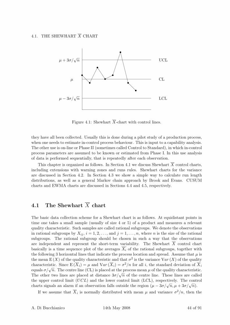
4.1. THE SHEWHART X CHART

s

@@s�

��s

JJJs��s�

��s

CCCCCCCCs@

@s

µ

µ + 3σ/√

n

µ− 3σ/√

n

CL

UCL

LCL

Figure 4.1: Shewhart X-chart with control lines.

they have all been collected. Usually this is done during a pilot study of a production process,when one needs to estimate in-control process behaviour. This is input to a capability analysis.The other use is on-line or Phase II (sometimes called Control to Standard), in which in-controlprocess parameters are assumed to be known or estimated from Phase I. In this use analysisof data is performed sequentially, that is repeatedly after each observation.

This chapter is organized as follows. In Section 4.1 we discuss Shewhart X control charts,including extensions with warning zones and runs rules. Shewhart charts for the varianceare discussed in Section 4.2. In Section 4.3 we show a simple way to calculate run lengthdistributions, as well as a general Markov chain approach by Brook and Evans. CUSUMcharts and EWMA charts are discussed in Sections 4.4 and 4.5, respectively.

4.1 The Shewhart X chart

The basic data collection scheme for a Shewhart chart is as follows. At equidistant points intime one takes a small sample (usually of size 4 or 5) of a product and measures a relevantquality characteristic. Such samples are called rational subgroups. We denote the observationsin rational subgroups by Xij , i = 1, 2, . . . , and j = 1, . . . , n, where n is the size of the rationalsubgroups. The rational subgroup should be chosen in such a way that the observationsare independent and represent the short-term variability. The Shewhart X control chartbasically is a time sequence plot of the averages Xi of the rational subgroups, together withthe following 3 horizontal lines that indicate the process location and spread. Assume that µ isthe mean E (X) of the quality characteristic and that σ2 is the variance Var (X) of the qualitycharacteristic. Since E (X i) = µ and Var (X i) = σ2/n for all i, the standard deviation of Xi

equals σ/√

n. The centre line (CL) is placed at the process mean µ of the quality characteristic.The other two lines are placed at distance 3σ/

√n of the centre line. These lines are called

the upper control limit (UCL) and the lower control limit (LCL), respectively. The controlcharts signals an alarm if an observation falls outside the region (µ− 3σ/

√n, µ + 3σ/

√n).

If we assume that X i is normally distributed with mean µ and variance σ2/n, then the


4.2. SHEWHART CHARTS FOR THE VARIANCE

probability of a false alarm equals

1− P (LCL < Xi < UCL | µ = µ0) = Φ(−3) + (1− Φ(3)) = 2(1− Φ(3)) ≈ 0.00270 ≈ 1

370.

If however the process mean shifts over a distance σ/√

n, then (see Exercise 4.16)

1− P (LCL < Xi < UCL | µ = µ0 ±σ√n

) ≈ 0.02278 ≈ 1

44.

In Phase I use of control charts, the centre line is placed at the overall mean of the observa-tions. The control limits are computed using (pooled) estimates of the variance from rationalsubgroups, often in terms of the range rather than the sample standard deviation. The relationbetween the range and the standard deviation is explored in detail in Section 4.2. In Phase IIuse of control charts, the values µ and σ are either known from historical data or estimatedfrom a capability study. In the latter case, it is not correct to apply the above calculation,although this is usually being ignored. For the effect of estimated parameters on the falsealarm probability we refer to Exercise 4.5. Shewhart based his choice for placing UCL andLCL at distance 3 times the standard deviation of group averages on practical experience. Itprovides a good compromise to a low false alarm rate and a quick detection of out-of-controlsituations. Explicit calculations will be discussed in Section 4.3.

4.1.1 Additional stopping rules for the X control chart

The decision rule to signal an alarm when a group average falls below the LCL or above theUCL is based on the current rational subgroup and ignores information from previous rationalsubgroups. In order to increase the detection performance of an X control chart, severaladditional stopping rules have been proposed.

Sometimes warning limits are added at distance 2σ/√

n of centre line. The idea of basingcontrol charts on different regions of observation values is also used in so-called zone controlcharts; for an example see Exercise 4.1. One of the proposed stopping rules using warninglimits is to signal an alarm if either a single group average falls outside the control limits or twosuccessive group averages both fall either above the upper warning limit or below the lowerwarning limit. Such a stopping rule is known in the SPC literature as a runs rule. Examplesof other runs rules include eight successive group averages below or above the centre line oreight increasing or decreasing group averages in a row. Often a combination of such rules isused. It is obvious that such combinations should be used with care, because they lead to anincrease in the false alarm rate. Explicit computations can be found in Section 4.3.

4.2 Shewhart charts for the variance

Since the normal distribution is completely specified by the parameters µ (mean) and σ2

(variance), it does not suffice to monitor the mean of a production process. Therefore it isgood practice to set up a control chart for the process variance in addition to the X controlchart. Both charts use the same rational subgroups. One would expect that the samplevariance is the natural choice for the statistic be monitored. However, because control chartswere devised by Shewhart in the pre-computer era, a simpler statistic, the range, was and isthe standard choice. The range R of a sample Y1, . . . , Yn is defined as

R := max1≤i≤n

Yi − min1≤i≤n

Yi = Y(n) − Y(1), (4.1)



where Y(i) denotes the ith order statistic. It can be shown that for small sample sizes, therange is performing almost as good as the standard deviation (see Exercise 4.8 which requiresresults from Subsection 4.2.1). Before we define control charts for the variance, we need tostudy the range and standard deviation.

4.2.1 The mean and variance of the standard deviation and the range

In this subsection we derive expressions for the mean and variance of the standard deviationand the range. These expressions are needed to set up control limits. If the observations Xij

are independent and normally distributed with mean µ and variance σ2, then the statistic(n − 1)S2

i /σ2 is χ2n−1 distributed. The expectation of

√n− 1 Si/σ is therefore (see also

Section 1.3) equal to∫ ∞

0

√t

1

2(n−1)/2 Γ((n− 1)/2)t(n−1)/2−1e−t/2dt =

√2

Γ(n/2)

Γ((n− 1)/2).

Hence,

E (Si) =

√2√

n− 1

Γ(n/2)

Γ((n− 1)/2)σ.

In particular, we have

c4(n) =

√2√

n− 1

Γ(n/2)

Γ((n− 1)/2).

Recall that Γ(1) = 1, Γ(1/2) =√

π and Γ(x + 1) = xΓ(x) for x 6= 0,−1,−2, . . .. Thisimmediately yields the following recursion for c4(n):

c4(n + 1) =

√n− 1√

n c4(n),

with the initial condition c4(2) =√

2/√

π. Note that the variance of Si can also be expressedin terms of c4(n) as defined in Section 3.4), because

Var (Si) = E (S2i )− (E (Si))

2 = σ2 − c24(n)σ2 =

(1− c2

4(n))σ2. (4.2)

We proceed by deriving an integral expression for E (Ri). Let F be the cumulative dis-tribution function of Xij . Then the distribution function of maxj(Xij) at y equals F (y)n

and of minj(Xij) at y equals 1 − (1 − F (y))n. We thus see that the expectation of Ri =maxj(Xij)−minj(Xij) equals

E (Ri) =

∫ ∞

−∞y

∂

∂y(F (y)n)− y

∂

∂y(1− (1− F (y))n) dy =

∫ ∞

−∞1− F (y)n − (1− F (y))n dy,

where the second equality follows from integration by parts. Note that the cumulative distribu-tion function F of a normal distribution with mean µ and variance σ2 equals F (y) = Φ

(y−µσ

).

We thus obtain

E (Ri) =

∫ ∞

−∞1− F (y)n − (1− F (y))n dy =

∫ ∞

−∞1− Φ

(y − µ

σ

)n

−(

1− Φ

(y − µ

σ

))n

dy.

Hence, a simple change of variables yields that for normally distributed samples we have

E (Ri) = σ

∫ ∞

−∞1− Φ(y)n − (1− Φ(y))n dy.



This integral must be computed numerically, since it has been proved that the distributionfunction of the standard normal distribution has no closed-form primitive. The proportionalityconstant is usually denoted by d2(n), i.e., E (Ri) = d2(n)σ. We conclude this subsectionwith the calculation of the variance of the range. It suffices to calculate E (R2), becauseVar (Ri) = E (R2

i ) − (E (Ri))2. Therefore we need to determine the joint distribution G of

(maxj(Xij), minj(Xij)). As before we denote with F (x) and f(x), the cumulative distributionfunction and the density, respectively, of the Xij

′s. We thus may write

G(x, y) = P{maxj

(Xij) ≤ x and minj

(Xij) ≤ y}

= P{maxj

(Xij) ≤ x} − P{maxj

(Xij) ≤ x and minj

(Xij) > y}

= F (x)n − (F (x)− F (y))n I{y<x}, (4.3)

where I{y<x} denotes the indicator function of the set {y < x}, which equals 1 if y < x and 0if y ≥ x. The joint density thus equals

∂2

∂x∂yG(x, y) = n(n− 1)(F (x)− F (y))n−2f(x)f(y) I{y<x}.

Hence,

E (R2i ) =

∫ ∞

−∞

∫ ∞

y(x− y)2n(n− 1)(F (x)− F (y))n−2f(x)f(y) dx dy

= −∫ ∞

−∞

∫ ∞

y2(x− y)n[(F (x)− F (y))n−1 − (1− F (y))n−1]f(y) dx dy

=

∫ ∞

−∞

∫ x

−∞2[(F (x)− F (y))n − (1− F (y))n + 1− F (x)n] dy dx

= 2

∫ ∞

−∞

∫ ∞

0[(F (y + r)− F (y))n − (1− F (y))n + 1− F (y + r)n] dr dy,

where the second and third equalities follow from integration by parts (note the special choiceof primitives, which causes some terms to vanish). If we take for F the cumulative distributionfunction Φ of the standard normal distribution, then we obtain that the expectation of R2

i isproportional to σ2. One usually writes

E (R2i ) =

(C(n)2 + d2(n)2

)σ2,

so that Var (Ri) = C(n)2σ2. Numerical calculation of the double integral E (R2i ) leads to

values of C(n).

4.2.2 The R control chart

The R control chart contains 3 lines. The centre line is placed at the expectation R0 of R,the range of a rational subgroup. If R0 is unknown, then one uses the estimator R of a phaseI study. In order to imitate the 3σ limits of the X control chart, it is convenient to introducesome notation. We throughout assume that the individual observations are independent andnormally distributed with mean µ and variance σ2. We will prove in this subsection that boththe mean and the standard deviation of the range are proportional to the standard deviation



n c4 d2 A2 D3 D4 D.001 D.999

2 0.7979 1.128 1.880 0.000 3.2673 0.8862 1.693 1.023 0.000 2.5754 0.9213 2.059 0.729 0.000 2.282 0.199 5.3095 0.9400 2.326 0.577 0.000 2.115 0.367 5.4846 0.9515 2.534 0.483 0.000 2.004 0.535 5.6197 0.9594 2.704 0.419 0.076 1.924 0.691 5.730

Table 4.1: Control chart constants.

of individual observations. The proportionality constants are denoted by d2(n) and C(n),respectively. I.e.,

E (R) = d2(n)σ (4.4)

Var (R) = C(n)2σ2. (4.5)

The upper and lower control limits are placed at 3 times the standard deviation of R. Theupper control limit, UCL, is placed at

R0 + 3√

Var (R) = R0 + 3C(n)σ =

(1 +

3C(n)

d2(n)

)R0.

One often writes D4(n) = 1 + 3C(n)/d2(n). The lower control limit, LCL, is similarly placedat D3(n)R0 with D3(n) = max(1−3C(n)/d2(n), 0). For an X control chart with control limitsbased on ranges one often defines A2(n) = 3/(

√n d2(n)), so the control limits are placed at

µ±A2(n)R. The range R is not normally distributed, so that alarm probabilities are not equalto 0.0027 as is the case for the X chart with known parameters. An alternative way to set upcontrol limits is based on quantiles of the range. These control limit are called probabilisticcontrol limits, defined as

UCL = D.999(n) Rd2(n) (4.6)

LCL = D.001(n) Rd2(n) . (4.7)

These limits are set up in such a way that the upper control limit UCL will be exceeded withprobability 0.001 The same holds for the lower control limit LCL. There exist tables of valuesfor Dγ(n). It would be logical to use the values Dγ and D1−γ with γ = 1 − Φ(3) ≈ 0.00135.The exceedance probabilities for both control limits are then equal. In practice this is notdone, because tables for Dγ usually do not include these values. The control limits based onthe .001 and .999 quantiles should be compared with 3.09 standard deviation control limits,because Φ(3.09) ≈ 0.999. We conclude this subsection with Table 4.1, which gives values ofsome control chart constants.

4.2.3 The S and S2 control charts

Alternatively, one may use the statistics S2i or Si to set up an S2 control chart or an S

control chart, respectively. The control limits for the S2 control chart follow easily because(n − 1)S2/σ2 follows a χ2

n−1 distribution. One may set up control limits at distance 3 timesthe standard deviation of S2 (see Exercise 4.9). An alternative is to use probabilistic controllimits as for the R control chart (see Exercise 4.9).


4.3. CALCULATION OF RUN LENGTHS FOR SHEWHART CHARTS

Control limits for the S control chart may be set up using (4.2). The centre line is placed atthe expectation σ of Si, the range of a rational subgroup. If this expectation is unknown, thenone uses the estimator S of a phase I study. The UCL is placed at σ + 3

√1− c4(n)2 σ

c4(n) =

B4σ. Likewise the LCL placed at σ − 3√

1− c4(n)2 σc4(n) = B3σ. Probabilistic control limits

may be obtained by taking square roots of the endpoints of two-sided confidence intervals forS2

i and replacing σ by σ/c4(n) (see Exercise 4.10).

By setting up appropriate control limits, all three types of control charts for the variancehave comparable false alarm probabilities. The difference in performance between these chartsis the ability to detect changes in the process variance. This is the topic of the next section.

4.3 Calculation of run lengths for Shewhart charts

The use of control charts in Phase I is retrospective in nature. In this phase it is most importantto detect whether out-of-control situations have occurred. A good control chart in Phase II(on-line use), however, should have a low false alarm rate and the ability to quickly detectout-of-control situations. The goal of this section is to put these properties into quantitativeterms. We will present two ways to perform calculations.

The way control charts are used is a special way of hypothesis testing. The difference withordinary one-sample testing is that control charts in phase II involve sequential testing, sinceeach time a new rational subgroup has been observed we again check whether the controlchart signals. In that sense the false alarm probability of an individual point on the controlchart is related to the type I error in hypothesis testing. The ability to detect process changesis related to the power of the test and thus to the type II error. For detailed discussionson the differences between control charts and hypothesis testing, we refer to Crowder et al.(1997), Stoumbos et al. (2000), Woodall (2000), and Woodall and Montgomery (1999). Inorder to incorporate the sequential character of control charts in phase II, the notions of typeI and II error are replaced by properties of the run length N , defined as the number of rationalsubgroups observed until the control chart signals an alarm. The most widely studied propertyof the run length is its mean. In the SPC literature one usually uses the term Average RunLength (ARL). One distinguishes between an in-control ARL (ARLin) and an out-of-controlARL (ARLout). Obviously, ARLin should be large (low false alarm rate or small type I error)and ARLout should be small (fast detection of changes, or high power ).

We now show how to compute ARL’s for Shewhart X-charts. It is obvious that if theprocess is in control (i.e., the distribution of the observations is normal with parameters thatcorrespond to the parameters used to set up the centre line and the control limits), each groupaverage of an X-chart has equal probability to fall outside the control limits. We denote thisprobability by p. Obviously P (N = n) = (1 − p)n−1p for p = 1, 2, . . .. Thus in this case Nhas a geometric distribution. Note that P (N > n) = (1− p)n. Hence,

EX =∞∑

n=0

P (N > n) =∞∑

n=0

(1− p)n =1

p.

Thus the ARLin of an X control chart equals 1/p = (Φ(−3) + 1− Φ(3))−1 ≈ 370. A similarcalculation yields that Var N = (1− p)/p2. Since N is nonnegative, it cannot be symmetric.Moreover, if p is small as is usual the case for control charts, then the standard deviation ofN almost equals its mean. The practical implication is that it may be very misleading to



judge the performance of a control chart by considering ARL’s only. Run length distributionsare usually highly skewed with large variability. The above calculation also holds for the R,S and S2 control charts if we use the appropriate values for p. Since it is recommended touse the X chart in conjunction with one of these three control charts for the variance, so theARL of interest should really be the ARL of the two used control charts (see Exercise 4.2 foran explicit calculation). Another issue that is often ignored is the fact that the process meanand variance are estimated, which may drastically change the run length distribution (seeExercise 4.16 for a simple example and Albers and Kallenberg (2004a), Albers and Kallenberg(2004b), Chakraborti (2000) and Ghosh et al. (1981) for further discussion).

Before we proceed by discussing run lengths of control charts with runs rules, we presenta general lemma, that may be useful for calculating the probability generating function ofnon-negative lattice distributions.

Lemma 4.3.1 Let X be a discrete random variable taking values on 1, 2, . . . and define

P (z) :=∞∑

j=1

P (X ≥ j) zj .

Then we have

a) P (z) = 1 +z − 1

zP (z) and P (z) = z

P (z)− 1

z − 1,

where P (z) is the probability generating function of X.

b) EX(m) = P (m)(1) = −m−1∑

k=0

m!

k!(−1)m−kP (k)(1),

where EX(m) = EX(X − 1)(X − 2) · · · (X −m + 1) is the mth factorial moment1 of X

and P (n) denotes the nth derivative of P .

In particular, EX = P ′(1) = P (1) and Var (X) = 2P ′(1)− P (1)− (P (1))2.

Proof.

a) We have

P (z) =∞∑

j=1

∞∑

k=j

P (X = k)zj

=∞∑

k=1

k∑

j=1

P (X = k)zj

=∞∑

k=1

P (X = k)zk+1 − z

z − 1

=z

z − 1

( ∞∑

k=1

P (X = k)(zk − 1

))

=z

z − 1(P (z)− 1).

1Here we follow the combinatorial convention, which differs from the convention in analysis and probability

theory. In combinatorics, one distinguishes between the lower factorial x(m) = x(x− 1) . . . (x−m + 1) and the

upper factorial x(m) = x(x + 1) . . . (x + m − 1)



Rewriting the above formula yields a).

b) The first equality is a basic property of probability generating functions. The secondequality follows by applying Leibniz’s formula for derivatives of products:

(f · g)(m) =m∑

k=0

(m

k

)f (k)g(m−k)

to a) and evaluating at z = 1. �

It has been mentioned in Subsection 4.1.1 that adding runs rules changes the ARL’s of aShewhart control chart. We start with a simple example that can be analyzed directly usinga recursion. Suppose we have an X chart with warning limits for which we agree that thechart signals if a point is outside the control limits or when there are two successive pointsbeyond either of the warning limits. Let p be the probability that a point of the control chartsfalls outside the control limits, q be the probability that a point falls between a control limitand the nearby warning limit (the warning region), and r be the probability that a point isbetween the two warning limits (the “safe” region). Obviously p + q + r = 1. Let L denotethe remaining ARL after a point in the good region and L′ the corresponding ARL after apoint in the warning region. If we start with a point in the safe region, then there are threepossibilities:

a) the next point is safe again, with probability r, and we expect L more points before analarm

b) the next point is in the warning region, with probability q, and we expect L′ more pointsbefore an alarm

c) the next point falls outside the control limits, with probability p, and we stop.

Note that we use that the statistics plotted on a Shewhart control chart are independent.Combining these three possibilities, we obtain

L = r(1 + L) + q(1 + L′) + p.

In a similar way we obtainL′ = r(1 + L) + q + p.

Combining these two equations, we obtain two linear equations with two unknowns. Hence,we may solve for L and L′. The ARL is then given by p + q(L + 1) + r(L′ + 1). Note thatsince we did not specify p, q and r the above derivation holds for both ARLin and ARLout.A similar way of reasoning yields ARL’s for other runs rules.

In order to obtain more detailed results on run length distributions, a different approachis necessary. We present a method from Brook and Evans (1972), which was first presented inthe context of run lengths for CUSUM charts. However, the method is very general and mayalso be applied to run lengths of Shewhart charts, as was first shown in Champ and Woodall(1987). The key in this approach is to represent the control chart as a Markov chain. In orderto illustrate the method, we consider an X control chart with the runs rule “two successivepoints outside the same warning limit”. We use a discrete-time Markov chain (Yk)k∈N withthe following four states:



State 1 Current point is in the safe region.

State 2 Current point is in the upper warning region, and the previous point was not.

State 3 Current point is in the lower warning region, and the previous point was not.

State 4 Current point is outside the control limits, or is in the same warning region as theprevious point (hence, the control chart signals).

Note that State 4 is an absorbing state. The probabilities of a point to fall into a certainregion are denoted as follows: p1: safe region, p2: upper warning region, p3: lower warningregion, and p4 = 1−p1−p2−p3 the action region (out-of-control situation). We thus have thefollowing transition matrix, where the rows denote the state before observing a new rationalsubgroup and the columns after observing a new rational subgroup:

P =

p1 p2 p3 p4

p1 0 p3 p2 + p4

p1 p2 0 p3 + p4

0 0 0 1

Now let Sk = (Sk,1, Sk,2, Sk,3, Sk,4) be the distribution of the state space after n observedrational subgroups, i.e., Sk,i = P (Yk = i). By the choice of states, the Markov property holds,so for k ≥ 1 we have that

Sk = Sk−1 P = S0 P k, (4.8)

where S0 = (p01, p02, p03, p04) is the initial probability distribution of the states. The defaultchoice for S0 is (1, 0, 0, 0) (but for other control charts this may not be the most naturalchoice). The run length distribution of N given the initial state distribution S0 may now becomputed from the relation

P (N ≤ k) = Sk,4. (4.9)

This relation can be easily programmed, but a closed form solution is preferable. Thereforewe partition the transition matrix P by singling out the absorbing state 4 as follows:

P =

(R p

0 1

),

where 0 denotes a vector of zeros. Hence, we have P k =

(Rk ck

0 1

). Since the rows of a

transition matrix sum to 1, it follows that ck = 1−Rk1 = (I−Rk)1. It follows from (4.8) and(4.9) that cki, the ith element of the vector (I−Rk)1, equals P (N ≤ k | first point is in state i)if 1 ≤ i ≤ 3. Hence, P (N > k | first point is in state i) equals the ith element of the vectorRk1. Now let N be the random vector, such that its ith element is the run length startingfrom state i with probability one. If we interpret the expression P (N > k1) as a shorthandfor the separate coordinate-wise inequalities, then we can compute E(N) as follows:

E(N) =∞∑

k=0

P (N > k1) =∞∑

k=0

Rk 1 = (I −R)−1 1.

The above expression not only gives an explicit formula for the ARL, but we also see that therun length distributions in a certain multivariate sense remains geometric (as was the case for


4.4. CUSUM PROCEDURES

the standard X control chart without runs rules). Further note that it is not always necessaryto perform matrix inversion (which may be numerically unstable), since in some cases thematrix R is nilpotent, i.e., there is an integer ℓ such that Rk = 0 for k ≥ ℓ.

For more calculations of run length distributions for Shewhart charts with runs rules, werefer to Champ and Woodall (1987), Champ and Woodall (1997), Does and Schriever (1992)and Fu et al. (2003) .

4.4 CUSUM procedures

As the basic statistical theory of testing was not developed until the 1950’s, Shewhart hadno choice but to develop simple monitoring tools. In this section we will show how likelihoodratios can be used to generate a class of sequential tests on which we can base control chartsthat are more sensitive to small changes. There is a close connection with a branch of statisticscalled changepoint analysis (see Hawkins et al. (2003)).

In order to better understand the background of sequential tests, we recall the well-knownNeyman-Pearson Lemma for simple alternatives. Assume that X1, . . . , Xn is a sample from adistribution with density fθ. In order to test

H0 : θ = θ0

versus

H1 : θ = θ1

define the likelihood ratio Λ by

Λn =fθ1(x1) . . . fθ1(xn)

fθ0(x1) . . . fθ0(xn). (4.10)

The Neyman-Pearson Lemma says that the test which rejects H0 if Λ > c for a certain valuek, has optimal power among all other tests of the same size, i.e., that have type I error lessthan or equal to PH0(Λ > c).

A sequential version of this test was developed by Wald during World War II. The idea isto repeatedly test the null and alternative hypotheses when data is being gathered, therebyhoping for a reduced sample size. Again we use the likelihood ratio defined by (4.10), but nown does not denote the fixed sample size, but the current sample size. The decision procedureis based on numbers a and b and reads:

accept H0 : if Λn ≤ a

accept H1 : if Λn ≥ b

continue sampling : if a < Λn < b.

The numbers a and b jointly determine the type I and II errors of this procedure, which canbe shown to terminate in finite time with probability 1. Wald and Wolfowitz proved thatthis test, which is called SPRT (Sequential Probability Ratio Test), is optimal with respectto the ASN (Average Sample Number), i.e., the average numbers of samples needed to reacha conclusion, among all tests with type I and II errors that do not exceed those of the SPRTat hand. Calculations of the ASN can be best performed by exploiting that the Λn’s form amartingale.



Control charts may be interpreted as sequential tests when we interpret the null hypothesisas being in-control and the alternative hypothesis as being out-of-control (see Lai (1995) andLai (2001)) for extensive discussions on this topic). A crucial difference with the SPRT is thatin a control chart setting we never accept the null hypothesis, but continue sampling. Thiscan be done by writing the loglikelihood ratio in a recursive form and resetting it to 0 whenthe null hypothesis is accepted. To formalize this, we write

log Λn =n∑

i=1

log

(fθ1(xi)

fθ0(xi)

)=

n∑

i=1

Zi. (4.11)

Then the CUSUM statistic Cn, first introduced in Page (1954), is defined by the recursion

Cn = max(0, Cn−1 + Zn), (4.12)

where C1 = 0. The CUSUM chart signals if the statistic exceeds a threshold (see examplebelow for details). The CUSUM has an optimality property in terms of an out-of-controlaverage run length.

CUSUM procedures can be developed for a wide range of distributions. For exponentialfamilies, the CUSUM procedures admit a convenient general from (see e.g., Chapter 6 ofHawkins and Olwell (1998). Rather than showing these general formulas, we illustrate thederivation of a CUSUM procedure for the case of a normal distribution with known varianceσ2. As null hypotheses we take

H0 : µ = µ0

versus

H1 : µ = µ1

A straightforward calculation using the elementary fact µ21 − µ2

0 = (µ1 − µ0) (µ1 + µ0) showsthat

Zi = − 1

2σ2

((xi − µ1)

2 − (xi − µ0)2)

=µ1 − µ0

σ2

(xi −

µ0 + µ1

2

).

If µ1 > µ0, then we have a so-called upper CUSUM chart C+n which signals if

C+n = max

(0, C+

n−1 + Xn −µ0 + µ1

2

)> h+. (4.13)

The value µ0+µ1

2 is called the reference value and is often denoted by k. If µ1 < µ0, then wehave a so-called lower CUSUM chart C−

n which signals if

C−n = max

(0, C−

n−1 −Xn +µ0 + µ1

2

)> h−. (4.14)

One usually simultaneously runs an upper and lower CUSUM chart. A recommended choicefor h+ and h− is 5σ, where σ is the standard deviation of an individual observation. Thevalue (µ0 + µ1)/2 in 4.13 and (4.14) is called k (warning: one sometimes measures h andk in terms of standard deviations). Unlike Shewhart charts, CUSUM are usually applied toindividual data. A refinement to improve the out-of-control ARL is not to restart at 0 but atanother value, e.g., at k. This idea was proposed in Lucas and Crosier (1982) and is calledFIR (Fast Initial Response). The rationale is that when the process is in-control, the value of



C+n will quickly return to 0, while in out-of-control situations it will take less time to exceed

the threshold h+.

Run length computations for the CUSUM chart are much harder than for the Shewhartcharts. The ARL’s are best calculated for the upper and lower CUSUM charts separately. Inthe sequel, we restrict ourselves to the upper CUSUM chart. The recursive form of the CUSUMshows that the conditional distribution of C+

n given the complete past equals the conditionaldistribution given C+

n−1. This fact was used in the seminal paper Brook and Evans (1972)by discretizing the range of C+

n into subintervals and setting up a Markov chain where thestates are these subintervals (see also William (1984)). Alternatively, one may derive integralequations for the ARL as in Page (1954); see Kemp (2001) for a lucid modern treatment.These integral equations usually can only be solved numerically. It can be shown that theMarkov chain method of Brook and Evans corresponds to a simple numerical integrationscheme corresponding to discretization at the midpoints of subintervals. Superior integrationschemes can be found in Hawkins (1992). Other papers of interest on this topic include Abeland Fuchs (1985), Gold (1989) and Jun and Choi (1993).

An important drawback of CUSUM schemes is that the ARLout−of−control may increasequickly for values that move away from the specific value of the alternative hypothesis that isused to construct the CUSUM. Therefore we now show how to extend the CUSUM procedureto handle composite alternative hypotheses by using generalized likelihood ratios. For a nicecomparison of the various principles that may be used to build control charts, we refer toHawkins et al. (2003). Instead of the simple sequential hypotheses studied above, we nowconsider hypotheses based on the following model. Assume we have observations (or derivedstatistics in case of rational subgroups) Xi with distribution function Fθ and density fθ, wherethe parameter θ belongs to a certain parameter space Θ.

H0,i : Xj ∼ Fθ (θ ∈ Θ0) for j ≤ i

H1,i : for some k < i

{Xj ∼ Fθ (θ ∈ Θ0) for j ≤ k

Xj ∼ Fθ (θ ∈ Θ1) for k < j ≤ i,

(4.15)

where Θ0∪Θ1 ⊂ Θ and Θ0∩Θ1 = ∅. The corresponding Generalized Likelihood Ratio statisticis

Λi = max1≤k<i

∏kj=1 supθj∈Θ0

fθj (xj)∏i

j=k+1 supηj∈Θ1fηj (xj)

∏ij=1 supθj∈Θ0

fθj (xj)= max

1≤k<i

∏ij=k+1 supηj∈Θ1

fηj (xj)∏i

j=k+1 supθ∈Θ0fθj (xj)

.

(4.16)The corresponding control chart is called the GLR control chart. Run length properties ofthis procedure have to be obtained by simulation.

In order to get more feeling for the flexibility of this setup, we consider some specificexamples of common out-of-control situations for normally distributed random variables. Foran extensive list of practical out-of-control situations in terms of patterns on means andvariances we refer to Chapter 8 of Gitlow et al. (1989) and Chapter 6 of Griffith (1996). Aslight variation on this control chart is the so-called cuscore chart. For a comparison of thesecharts, we refer to Runger and Testik (2003).



Persistent change of mean of given minimal size (σ, µ0 and δ > 0 known)

H0,i : µ1 = . . . µi = µ0

H1,i :

{µj = µ0, j = 1, . . . , k,

µj > µ0 + δ, j = k + 1, . . . , i,

(4.17)

In this case (4.16) is evaluated as follows:

log Λi = max1≤k<i

supµ>µ0+δ

i∑

j=k+1

−(xj − µ)2 + (xj − µ0)2

= max1≤k<i

i∑

j=k+1

−(xj −max(xj , µ0 + δ))2 + (xj − µ0)2

Writing Ti = log Λi and Wj = −(xj − max(xj , µ0 + δ))2 + (xj − µ0)2, we have that Ti =

max1≤k<i∑i

j=k+1 Wj . Now observe that the terms over which the maximum is taken in Ti+1

are the same terms as for Ti with the addition of the extra term Wi+1 resulting from the casek = i. The terms in Ti+1 for k < i differ by Wi+1 from the corresponding term occurring inthe maximum for Ti. This explains the following derivation of a recursion for TI :

Ti+1 = max1≤k<i+1

i+1∑

j=k+1

Wj

= max

max

1≤k<i

i+1∑

j=k+1

Wj

, Wi+1

= max

max

1≤k<i

Wi+1 +

i∑

j=k+1

Wj

, Wi+1

= Wi+1 + max

max

1≤k<i

i∑

j=k+1

Wj

, 0

= Wi+1 + max(Ti, 0).

Epidemic alternative (σ, µ0 and δ known)

H0,i : µ1 = . . . = µi = µ0

H1,i :

µj = µ0, j = 1, . . . , ℓ,

µj = µ0 + δ, j = ℓ + 1, . . . , m,

µj = µ0, j = m + 1, . . . , i

(4.18)

Persistent non-monotone threshold crossing of mean (σ and δ known)

H0,i : µj ≤ δ, j = 1, . . . , i,

H1,i :

{µj ≤ δ, j = 1, . . . , k,

µj > δ, j = k + 1, . . . , i,

(4.19)


4.5. EWMA CONTROL CHARTS

A monotone version of this situation has been studied in Chang and Fricker (1999). Thissituation is a good model for tool wear.

Persistent monotone threshold crossing (σ and δ known)

H0,i : µ1 ≤ . . . ≤ µi ≤ δ

H1,i :

{µ1 ≤ . . . ≤ µk < δ j = 1, . . . , k

δ < µk+1 ≤ µk+2 ≤ . . . ≤ µi j = k + 1, . . . , i

(4.20)

Of course, it also possible to consider alternative hypotheses concerning the variance.

Persistent non-monotone threshold crossing of variance (σ and δ known)

H0,i : σj ≤ δ, j = 1, . . . , i,

H1,i :

{σj ≤ δ, j = 1, . . . , k,

σj > δ, j = k + 1, . . . , i,

(4.21)

4.5 EWMA control charts

The EWMA (Exponentially Weighted Moving Average) chart is based on ideas from Girshickand Rubin (1952), Roberts (1959) and Shiryaev (1963). The inspiration comes by Bayesiananalysis by putting a prior distribution on the changepoint. The chart is defined by therecursion

Vi = λXi + (1− λ)Vi−1, V0 = 0 and 0 < λ < 1. (4.22)

It is easy to see that when λ → 0, then we obtain a CUSUM procedure, while for λ = 1we recover a Shewhart chart. A recommended choice for λ is 0.1 < λ < 0.3. Run lengthcalculations require numerically solving integral equations (?, Gan and Chang (2000)), orapplying the Brook-Evans method after discretization (see Calzada and Scariano (2003) forthe link between these two approaches). The main advantages of the EWMA chart are thatits performance in terms of detecting small changes is nearly as good as for CUSUM chartsand the robustness against deviations from normality. A disadvantage compared to Shewhartcharts is that the control limits change over time, although it must be said that they convergerather quickly.

4.6 Exercises

Exercise 4.1 Let L < U be given real numbers. Assume that instead of the actual outcomesX1, . . . , Xn of a sample from a normal distribution we only have information on the numbers ofoutcomes that fall below L, fall between U and L, and fall above U . Find Maximum Likelihoodestimators for µ and σ2 based on this information only. This is used in so-called gauge controlcharts. The idea goes back to Stephens (1948); for modern accounts we refer to Farnum andStanton (1986) and Farnum and Stanton (1991)).

Exercise 4.2 A standard Shewhart X chart has an in-control ARL equal to 370. What is theARL of a combined Shewhart X and S2-chart, when we use probabilistic control limit so thatalso the S2-chart has an in-control ARL of 370?


4.6. EXERCISES

Exercise 4.3 The data set ceramic.txt contains measurements of electrical characteristics ofassemblies during a pilot study of a new production process. The measurements were collectedeach half hour in rational subgroups of size 7. The production manager wishes that the averagetime to detect a shift of the mean of size 0.7 should be 2 hours. Suggest an appropriate controlchart and a corresponding sampling strategy.

Exercise 4.4 A quality characteristic of a certain production process is known to be normallydistributed with σ = 4. In order to obtain a good quality of the products, it is required to detectchanges in the mean of 4 units. Currently rational subgroups are taken every 15 minutes.

a) What is the necessary minimum size of the rational subgroups if the mean detection timeis 1 hour?

b) What should be the sampling frequency if the producer wishes to be 90% certain of de-tecting changes in the mean of 4 units within 1 hour?

Exercise 4.5 Assume that a capability study has been performed with N observations, subdi-vided into m rational subgroups of size n = N/m. In the subsequent Phase II, a Shewhart Xchart has been set up based on rational subgroups of size n. The control limits are set at set

at a distance of 3S =√

1N

∑mi=1 S2

i .

a) Assume that the centre line is set at the known process mean. Compute the probabilitythat a group average falls outside the control limits. Compare your result with the well-known probability 0.0027 when N ranges from 50 to 100.

b) Repeat your calculations for the case that the centre line is set at the overall mean fromthe capability study. Compare your results with a) and the standard 0.0027 probabilityfor the same ranges of N .

c) The above results are independent of n. May we therefore conclude that the choice of nis unimportant?

Exercise 4.6 A laboratory always performs an analysis of a certain process characteristic induplicate. Discuss whether one should use the individual values or the average value on aShewhart X chart.

Exercise 4.7 Write a program in R to produce of table of d2(n). Hint: use the functionintegrate.

Exercise 4.8 Study the relative efficiency ( i.e., the ratio of the variances) of the unbiasedestimators S/c4(n) and R/d2(n) for σ when we sample from a normal distribution. For whichvalues is R/d2(n) a reasonable alternative for S/c4(n)? Hint: use the function adapt in theadapt package to evaluate Var (R).

Exercise 4.9 a) Show that Var S2 = σ4/(n− 1)2 when the observations form a sample ofsize n from a normal distribution. Use this to derive control limits placed at a distanceof 3 times the standard deviation of the sample variance.

b) Derive probabilistic control limits for the S2 control chart.


4.6. EXERCISES

Exercise 4.10 a) Set up an S control chart by placing control limits at a distance of 3times the standard deviation of the sample standard deviation.

b) Derive probabilistic control limits for the S control chart. Hint: use a two-sided confi-dence interval for the variance and take square roots of the end-points.

Exercise 4.11 Write a program in R to produce a table of D0.00135 and D0.99875.

Exercise 4.12 A production process has been running for a long time, during which data hasbeen gathered and analysed. The conclusion is that under stable conditions, the process has amean of 64 and a standard deviation of 0.02. Consider the data set monthlyreport.txt oflast month’s production. Your task is to report to the Quality Supervisor. What should youreport? Give a clear motivation for your report.

Exercise 4.13 In an injection moulding process it is important to keep part weight consistentover time. Therefore control charts are applied to monitor part weight. The data collectionconsists of taking 5 consecutive parts per shift and obtaining the weight of each part. The dataset injectionmoulding.txt contains averages and range of the rational subgroups.

a) Report through appropriate control charts on the moulding process. Do not forget tocheck the assumptions on which your control charts are based.

b) Subsequent investigations of the process revealed nothing unusual on the conditions duringthe data collection. Moreover, subsequent runs with the same unchanged process turnedout parts that were consistently acceptable. How can this be explained?

c) Use the sample averages as individual observations and construct a control chart forindividual observations. Interpret this new control chart. Compare your results with theprevious control charts.

Exercise 4.14 Give a formal justification of the conditional arguments with average runlengths in the first halve of Section 4.3.

Exercise 4.15 Compute ARLin for an X control chart with the extra runs rule “two out ofthree successive point outside either warning limit”.

Exercise 4.16 Consider the standard assumptions of the Shewhart X-chart with rational sub-groups of size n.

a) What is the probability that 2 out of 3 consecutive observations fall in the region (µ0 −2σ/√

n, µ0 + 2σ/√

n), if the individual observations are independent and normally dis-tributed with expectation µ0 and variance σ2?

b) What is the alarm probability for a single group mean Xi if Xi is normally distributedwith expectation µ0 + σ/

√n and variance σ2/n?

c) We would like to change the control limits µ0 ± 3σ/√

n into µ0 ± kσ/√

n. Which valueshould we choose for k in order to achieve that the probability of a single group meanX i falling outside the control limits equals 0.01? Assume that Xi is normally distributedwith expectation µ0 and variance σ2/n.


4.6. EXERCISES

Exercise 4.17 The lifetimes of certain parts of a machine need to be replaced often. Onewishes to monitor the quality of the parts by monitoring the life times of these parts. Prac-tical experience from the past indicate that lifetimes can be assumed to follow an exponentialdistribution. A recent sample has been taken and is presented in lifetimes.txt. The unit isdays.

a) Derive an upper 95%-mean tolerance interval for the life times.

b) In order to monitor the replacement frequency of the parts, one wishes to set up a She-whart X chart with 3σ control limits. Compute the centre line and the control limits ofsuch a control chart, if we assume that the observations in the sample correspond to anin-control situation.

c) Indicate one or two problems in setting up such a Shewhart-like chart for this situation.

d) Derive a one-sided CUSUM procedure based on an SPRT procedure when the in-controlmean equals 5 days and one wishes to detect an out-of-control mean equal to 3 days.

Exercise 4.18 Suppose that apart from the standard out-of-control criterion (“one observationoutside the control limits”) we also use the following runs rule on a Shewhart X chart: twosuccessive points at distance 2σX or more from the centre line. Compute the ARLin-control forthis control chart.

Exercise 4.19 Compute the in-control Average Run Length of a standard Shewhart X-chartwith 3σ control limits if we add the runs rule “alarm if 3 consecutive observations on the sameside of the centre line”.

Exercise 4.20 An EWMA control chart is defined in terms of moving averages as follows:Vi = λXi + (1− λ)Vn−1, where V0 = µ and 0 < λ < 1. Prove that

V3 = (1− λ)3µ + λ(1− λ)2X1 + λ(1− λ)X2 + λX3.

Assume that the observations X1, X2, X3 are independent with expectation µ and varianceσ2. Calculate the expectation and variance of Z3.


Chapter 5

Solutions Exercises Historical

Introduction to SPC

Solution of Exercise 1.1The three methods of managing variation mentioned in the text are

Fitness for use In ancient times, products were simple and unique. Usually one craftsmanwas one craftsman responsible for the product, there were no specifications or designs.The item was inspected and worked until it was assessed by the craftsman to be fit foruse.

Specification and tolerance Specifications and tolerances were necessary to communicatebetween industries and define what should be delivered.

Control chart The control chart is a statistical tool, which is used to distinguish betweenvariation in a process due to common causes and variation due special causes.

Solution of Exercise 1.2The test methods mentioned in the text are

• inspection by a craftsman

• subjective inspection by an inspector, who disassembles and reassembles the product,and tests for functionality.

• objective inspection through gauges

• use of specifications, dimensioned tolerances and standards.

Solution of Exercise 1.3The products were simple and unique. The craftsman worked at the crafted item until it wasfit for his use.

Solution of Exercise 1.4Variation became a critical issue through the development of the concept of interchangeable

61

parts. With the later rise of mass production, variation became even more critical becauseinspection turned to be too expensive.

Solution of Exercise 1.5The reason that standards for inspection were formulated was the rise of mass production.

Solution of Exercise 1.6Gauges are set to specify when a product must be rejected. If the product satisfies the gauges,then the product is a go. It can be shipped and sold. When the product does not satisfy thegauge, the product is a no-go and will be rejected.

Solution of Exercise 1.7The goal of setting tolerances and specifications is to get a more objective inspection system. Italso facilitates the communication between industries. Specifications are necessary to describequality characteristics.

Solution of Exercise 1.8Interchangeability means that a part or component of the product can be replaced by anotherpart of component and maintain the same function. The interchangeable parts must satisfythe same specifications. Examples of “modern” products with interchangeable parts includebicycles, televisions and computers.

Solution of Exercise 1.9It is necessary that there is as little as possible variation in the interchangeable components.If there is too much variation, components will no longer be interchangeable.

Solution of Exercise 1.10The goal of a control chart is to distinguish between variation in a process due common causesand special causes. Special causes can be identified and should be removed.

Solution of Exercise 1.11The approach based on setting specifications focuses on quality of individual products. Thefocus of Shewhart’s approach is performance of the process. There is no relationship betweenthe two approaches. A process can be out of statistical control, but all of its outcomes maybe within specifications.

Solution of Exercise 1.12Shewhart determined through practical experience empirical that control limits at a distanceof 3 standard deviations perform well. If the distance is smaller than 3σ, then the controlchart indicates too often that the process is out of control. This results in an overreaction (toomany false alarms). If the distance is bigger than 3σ, then the control chart indicates too latethat the process is out of control. This may result in an unnoticed out of control situation.

Solution of Exercise 1.13Taguchi presented the idea that any variation from a desired target is a loss to society. Taguchiargues that specification limits does not seem to reflect reality, because a product becomesgradually worse when it deviate from the desired target. He therefore thinks that the idea thatloss somehow jumps in value at specification limits does not seem to reflect the real world.


Solution of Exercise 1.14If the variation in critical parameters of parts is too big, the parts will not fit because thereis an accumulation of tolerances. This is called tolerance stack-up.


Chapter 6

Solutions Exercises Introduction to R

Solution of Exercise 2.1

pchisq(5.2, df=3, lower.tail=FALSE)


qnorm(0.99)


dataset <- rnorm(100, mean = 10, sd = sqrt(2))

hist(dataset, breaks=10, xlab="10 bins")

hist(dataset, breaks=20, xlab="20 bins")

# A more automated way of playing can be made as follows;

histdemo <- function(data,numberofbins=floor(sqrt(length(data))))

{

hist(dataset, breaks= numberofbins, xlab= paste("number of bins = ",numberofbins))

}

qqnorm(dataset), qqline(dataset) # adds line through 1st and 3rd quartile

shapiro.test(dataset) # Shapiro-Wilks test for normality

t.test(dataset, alternative=c(‘‘two.sided’’),conf.level=0.95,mu=10)

# test for variance does not exist in R, we test using confidence interval:

n <- length(dataset)

65

c((n-1)*var(dataset)/qchisq(0.975,df=n-1),(n-1)*var(dataset)/qchisq(0.025,df=n-1))

# alternative: test with critical region

if( (n-1)*var(dataset)/2 >= qchisq(0.975,df=n-1)

|| (n-1)*var(dataset)/2 <= qchisq(0.025,df=n-1))

c("Reject that variance is equal to 2")

else c("Do not reject that variance is equal to 2")


dataset <- rexp(10, rate=1/3)

mean(dataset) # check whether parametrization is right

Solution of Exercise 2.10The following implementation is not very efficient, but has the advantage of showing someuseful features of R like deparse, apply and the use of anonymous functions. The functionabline draws lines with a given intercept and slope.

Weibullplot <- function(data,shapepar,scalepar,

nameofdata=deparse(substitute(data)))

{

n<-length(data)

orderstat <- sort(data)

quantiles <- sapply(seq(1:n)/(n+1),

(function(x) qweibull(x,shape=shapepar,scale=scalepar)))

plot(orderstat,quantiles,main=paste("Weibull plot of", nameofdata) ,

xlab=paste("Sample quantiles of", nameofdata),

ylab=paste("Quantiles of Weibull (",shapepar,",",scalepar,") distribution"),

abline(0,1) )

}

A more efficient solution would be to use the internal function ppoints and the fact thatqweibull is threadable over lists.

Weibullplot2 <- function(data,shapepar,scalepar,

nameofdata=deparse(substitute(data)))

{

plot(sort(data),qweibull(ppoints(data),shape=shapepar,scale=scalepar),

main=paste("Weibull plot of", nameofdata) ,

xlab=paste("Sample quantiles of", nameofdata),

ylab=paste("Quantiles of Weibull (",shapepar,",",scalepar,") distribution") ,

abline(0,1))

}

The data sets can be generated using

data1 <- rweibull(30,shape=3,scale=2)

data2 <- rgamma(30,shape=7.57, rate=0.235)


Chapter 7

Solutions Exercises Process Capability

Analysis

Solution of Exercise 3.1We write d = 1

2(USL− LSL), so d/σ = 3Cp .

a) Since the process is centred, standardization of X (see Formula (3.2)) yields that thepercentage non-conforming items equals

P (X < LSL) + P (X > USL) = 2Φ(−d/σ) = 2Φ(−3 Cp) = 2Φ(−3.99) = 0.000066.

b) If µ = (2USL + LSL)/3, then in the same way we obtain that

P (X < LSL)+P (X > USL) = Φ(−4Cp)+Φ(−2Cp) = Φ(−5.32)+Φ(−2.66) = 0.0039.

Alternatively, we may use (3.3)

Cpk =

(1− | µ− 1/2(LSL + USL) |

d

)Cp =

(1− 1/6 | USL− LSL |

1/2 | USL− LSL |

)=

2

3Cp .

The expected proportion non-conforming items can thus by (3.5) be expressed as

P (X < LSL)+P (X > USL) = Φ(−3(2Cp−Cpk))+Φ(−3 Cpk) = Φ(−5.32)+Φ(−2.66) = 0.0039.

Solution of Exercise 3.2By Theorem 3.5.2, we have

√n(σ2 − σ2)

d−→ N(0, 2σ4

). Applying Theorem 3.5.1(Cramér)

with g(x) = x− 12 , we obtain

√n

(1

σn− 1

σ

)→ N

(0, 2σ4

( −1

2σ3

)2)

= N

(0,

1

2σ2

).

Since Cp = USL−LSL6bσ , it follows that

√n(Cp − Cp)→ N

(0,

(USL− LSL)2

72σ2

).

67

Solution of Exercise 3.3We first derive an exact confidence interval for Cp for normal samples. The ML estimator for

σ equals σ =√

1n

∑ni=1(Xi −X)2. Recall that n σ2

σ2 ∼ χ2n−1. Hence,

P

(χ2

n−1,α/2 ≤nσ2

σ2≤ χ2

n−1,1−α/2

)= 1− α

By the Invariance Principle (Theorem 3.3.2) we have that Cp/Cp = σ/σ. Substituting thisinto the above defining relation for a confidence interval for σ2, we obtain

P

(χ2

n−1,α/2 ≤nC2

p

Cp2 ≤ χ2

n−1,1−α/2

)= 1− α.

Hence, an exact 100 (1− α)%-confidence interval for Cp equals

√χ2

n−1,α/2

nCp,

√χ2

n−1,1−α/2

nCp

.

We now derive an asymptotic confidence interval for Cp. We derived in Exercise 3.2 that

√n(Cp − Cp)→ N

(0,

(USL− LSL)2

72σ2

).

Since nσ2/σ2 ∼ χ2n−1 and the χ2

n−1 can be realized as the sum of n − 1 standard normalrandom variables, continuity of the function

√x and the Strong Law of Large Numbers imply

that σ/σ converges in probability to 1. Hence, Slutsky’s Lemma implies that we also have

√n(Cp − Cp)σ → N

(0,

(USL− LSL)2

72

).

Hence, for large n we have

P

(−zα/2 ≤

√72nσ2(Cp − Cp)

USL− LSL≤ zα/2

)≈ 1− α

A 100 (1− α)%-confidence asymptotic interval for Cp is thus given by

[Cp − zα/2

USL− LSL√72nσ2

, Cp + zα/2USL− LSL√

72nσ2

]

These confidence intervals can be implemented in R in the following way:

CpCIexact <- function(data,LSL,USL,alpha=0.05){

n<-length(data)

Cpest <- (USL-LSL)/(6*sd(data))

c(Cpest*sqrt(qchisq(alpha/2,df=n-1)/(n-1)),


Cpest*sqrt(qchisq(1-alpha/2,df=n-1)/(n-1)))

}

CpCIasymptotic <- function(data,LSL,USL,alpha=0.05){

n<-length(data)

Cpest <- (USL-LSL)/(6*sd(data))

c("Cp = ",Cpest,100*(1-alpha)," % confidence interval=",

Cpest-qnorm(1-alpha/2)*(USL-LSL)/sqrt(72*n*var(data)),

Cpest+qnorm(1-alpha/2)*(USL-LSL)/sqrt(72*n*var(data)))}


Since the N(µ, σ2) distribution has cumulative distribution function F (u) = Φ

(u− µ

σ

), it

follows that Φ

(b− X

σ

)−Φ

(a− X

σ

)= F (µ+ b−X)−F (µ+a−X). By Proposition 3.6.7,

we have

E

[Φ

(b−X

σ

)− Φ

(a−X

σ

)]= P (µ + a−X < X < µ + b−X)

= P

(a− µ

σ√

1 + 1/n<

X + X − 2µ

σ√

1 + 1/n<

b− µ

σ√

1 + 1/n

)

= Φ

(b− µ

σ√

1 + 1/n

)− Φ

(b− µ

σ√

1 + 1/n

),

where we because of independence we have that V ar(X − X) = (1 + 1/n)σ2. Hence,

Φ

(b−X

σ

)− Φ

(a−X

σ

)is a biased estimator for P (a < X < b), but the bias vanishes

as n→∞

Solution of Exercise 3.5Note the use of apply in the solution which avoids a loop. It is almost always possible toavoid loops. Loops may be slow because they are memory consuming.

MLconf <- function(a,b,data){

n <- length(data)

pt((b-mean(data))/sd(data),df=n-1)-pt((a-mean(data))/sd(data),df=n-1)}

UMVUconf <- function(a,b,data){

n <- length(data)

pt(sqrt(n/(n-1))*(b-mean(data))/sd(data),df=n-1)-

pt(sqrt(n/(n-1))*(a-mean(data))/sd(data),df=n-1)}

simulationloop <- function(iterations=100,size,a,b,mu=0,var=1){

truevalue <- pnorm((b-mu)/sqrt(var))-pnorm((a-mu)/sqrt(var))

setup <- matrix(c(iterations,size,mu,var,a,b,truevalue),nrow=1)

dimnames(setup) <- list("",c("iterations","sample size", "mean",


"variance","a","b", "P(a<X<b)"))

print(setup,print.gap=2)

cat("\n") # empty new line

sample <-matrix(rnorm(size*iterations,mean=mu,sd=sqrt(var)),nrow=iterations,

byrow=T)

MLestim <-apply(sample,1,function(x) MLconf(a,b,x))

UMVUestim <-apply(sample,1,function(x) UMVUconf(a,b,x))

resultsML <- matrix(c(truevalue,mean(MLestim),sd(MLestim),

truevalue-mean(MLestim),sd(MLestim)+(mean(MLestim)-truevalue)^2),nrow=1,

byrow=T)

resultsUMVU <- matrix(c(truevalue,mean(UMVUestim),sd(UMVUestim),

truevalue-mean(UMVUestim),

sd(UMVUestim)+(mean(UMVUestim)-truevalue)^2),nrow=1,byrow=T)

results <- rbind(resultsML,resultsUMVU)

dimnames(results) <- list(c("ML estimator", "UMVU estimator"),

c("true", "average", "st. dev.", "bias","MSE"))

print(results,digits=3,print.gap=2)

}

Solution of Exercise 3.6Assume without loss of generality that the process has shifted to the right, i.e, µ = (USL+LSL)

2 +δ with δ > 0. Hence, in this case

Cp k = min

(USL− µ

3σ,µ− LSL

3σ

)= min

(USL−LSL

2 − δ

3σ,

USL−LSL2 + δ

3σ

)

=USL− LSL

6σ− δ

3σ

= Cp −δ

3σ= 2− δ

3σ= 1.67.

The conclusion is that the long-term shift in the mean equals σ.

Solution of Exercise 3.7By Exercise 3.3, a 100 (1− α)%-confidence asymptotic interval for Cp equals

[Cp − zα/2

USL− LSL√72nσ2

, Cp + zα/2USL− LSL√

72nσ2

],

we get that zα/2USL−LSL√

72nσ2= 0.1 and α = 1− 0.95 = 0.05. Hence,

n = z20.025

(USL− LSL)2

0.72σ2.

Solution of Exercise 3.8All calculations are based on the assumption that the observations are independent and are


distributed according to the same normal distribution. The statistic (n − 1) c20/Cp

2= (n −

1)S2/σ2 has a χ2n−1 distribution. Hence,

PH0

(Cp > kc0

)= PH0

(Cp

c0> k

)

= PH0

(c20

Cp2 < 1/k2

)

= PH0

((n− 1)

c20

Cp2 <

n− 1

k2

)

= P

(χ2

n−1 <n− 1

k2

)= α.

Hence, k =

√χ2

n−1;1−α

n−1 yields a test with type I error equal to α with corresponding critical

region

{Cp <

√n−1

χ2n−1;1−α

c0

}. The power function is given by

P

(Cp <

√n− 1

χ2n−1;1−α

c0 | Cp = c

)= P

(Cp

c<

√n− 1

χ2n−1;1−α

c0

c

∣∣∣∣∣Cp = c

)

= P

((n− 1)Cp

2

c2< χ2

n−1;1−α

(c

c0

)2)

= P

(χ2

n−1 < χ2n−1;1−α

(c

c0

)2)

.

Solution of Exercise 3.9To be written.

Solution of Exercise 3.10To be written.


a) The individual data are not normally distributed, but the group means are. To assesswhether the production data show a process that is in statistical control, we may there-fore safely use the group means. To assess capability, we must use individual data, butcannot rely on the standard capability indices, since these indices assume normality.

b) We see from the data set that the subgroups have sample size 4. To assess whetherthe process in statistical control, we must do an analysis based on control charts withµ = 5.12 and σ = 0.023. For sake of simplicity, further analysis is based on the standard3σ -rule, and does not use further runs rules. We first look at the range chart, since themean chart is based on the assumption that the variance is stable. The process seems


to be in statistical control until group 15. We assume that this has to do with a specialcause (in practice this should be investigated, of course). Since we do not know whathas happened after subgroup 15, we decide to be on the safe side and restrict furtheranalysis to the first 14 subgroups (= first 56 individual data). Both charts now indicatethat the process is in statistical control.

c) The capability indices must be calculated using data from a process that is in statisti-cal control, hence restricted to the first 14 subgroups. With the individual data fromsubgroup 15 deleted, the individual data are now normal. Hence, we may safely usethe standard capability indices that are based on a normality assumption. The 95%confidence intervals are: Cp = (1.45, 2.12), Cpk = (1.37, 2.03).

d) 0.000018% is predicted to fall outside the specification limits.

e) Based on the predicted fall-out, the histogram and the point estimates for the capabilityindices (both around 1.7) capability seems to be in order. However, too much optimismis dangerous since the 95% confidence intervals are wide, a result of not consideringenough data. Moreover, a look at the density trace (kernel estimator for the density)reveals that the right-end tail of the distribution seems to be missing. This should beinvestigated.

f) The process is definitely not capable of meeting these stricter specifications. This canbe seen from the dramatically low capability indices (less than 1). The process seems tobe on target, but the variance is much too high. An improvement plan for reducing thevariance of the process must be set up. Probably drastic changes and/or redesign of theprocess are necessary.

Solution of Exercise 3.12A major problem is that the data given only consists of group summary statistics, not theindividual data. Thus a reliable capability analysis is not possible. Ignoring this for themoment, we see that the process is not in statistical control. Something is wrong with subgroup10. If we remove the data from subgroup 10, then both the mean and range charts indicatethat the process is in statistical control. Normality tests indicate that there is no reasonto doubt that the means come from a normal distribution. Capability analysis shows thatboth the actual capability and the potential capability are too small. The process is not wellcentred around the target and the variance is much too high. Although centring the process isrelatively easy, the plant manager should first try to reduce variation rather than first centringthe process around the target. This is because with such a high variance, it is not assuredthat the process will stay centred.

Solution of Exercise 3.13The likelihood equals θn (

∏ni=1 xi)

θ−1. The factorization Lemma thus yields that∏n

i=1 Xi asufficient statistic for θ.

Solution of Exercise 3.16Since µ is known and σ2 is known, we try an interval of the form [µ−kS, µ+kS]with k suchthat

E (F (µ + kS)− F (µ− kS)) = β.


By Proposition 3.6.7 we get that

E (F (µ + kS)− F (µ− kS)) = P (µ− kS < X < µ + kS) = β.

where X ∼ N(µ, σ2) and then X−µS ∼ Tn−1

Since

P (−k <X − µ

S< k) = β

Hence, we get that k = tn−1, 1−β

2.

Solution of Exercise 3.17Since µ is known, and σ2 is unknown, we try an interval of the form [µ− kS, µ + kS] with ksuch that

P ((Φ(kS/σ)− Φ(−kS/σ)) ≥ β) = α.

If Φ(kS/σ)− Φ(−kS/σ) ≥ β, we get that kS/σ ≥ z 1−β2

. So we have

P(kS/σ ≥ z 1−β

2

)= α = P

((n− 1)S2/σ2 ≥ z2

1−β2

(n− 1)/k2

)

Since (n− 1)S2/σ2 ∼ χ2n−1, we get that

(n−1)Z21−β

2k2 = χ2

n−2,α. Hence,

k =z 1−β

2

√n− 1

√χ2

n−1,α

.


Chapter 8

Solutions Exercises Control Charts

Solution of Exercise 4.1Rather than trying to write down the likelihood equations directly which leads to a cumber-some expression, we invoke the Invariance Principle (Theorem 3.3.2). We first write

nL = |{i : Xi ≤ L}|nU = |{i : Xi ≥ U}|.

Recall that nL/n and nu/n are the Maximum Likelihood estimators for P (X ≤ L) andP (X ≥ U), respectively. It follows from the Invariance Principle (Theorem 3.3.2) that

nL

n= P (X ≤ L) =

Φ

(L− µ

σ

)= Φ

(L− µ

σ

).

andnU

n=

Φ

(µ− U

σ

)= Φ

(µ− U

σ

),

where µ and σ denote the Maximum Likelihood estimators based on nL and nU , respectively.Hence,

L− µ

σ= Φ−1(nL/n)

µ− U

σ= Φ−1(nU/n).

If we solve this system of equations with respect to µ and σ, then we obtain

σ =L− U

Φ−1(nL/n) + Φ−1(nU/n)

µ = L +(U − L)ϕ−1(nL/n)

Φ−1(nL/n) + Φ−1(nU/n).

Solution of Exercise 4.2Use the fact that for normal samples, the statistics X and S2 are independent. The probability

75

that both control charts are in control is for probabilistic control limits equal to (1−0.0027)2.Hence, the probability that at least one of them is out of control at a specific point in timeequals 1− (1−0.0027)2 ≈ 1/185. The ARL of the combined chart is thus approximately equalto 185.




Solution of Exercise 4.6It is best to put average values on the Shewhart chart, because otherwise one would ob-tain a biased estimate of the process variance: the variance of individual values also containcontributions to measurement errors.

Solution of Exercise 4.7Although R is aimed at statistical calculations rather than numerical calculations, it is noproblem to produce a reliable table for d2(n).

d2integrand <- function (y,n){1 - pnorm(y)^n - (1-pnorm(y))^n}

d2 <- function(n){integrate(function(y){d2integrand(y,n)},-Inf,Inf)$value}

# integrate returns a vector;

# the component value of that vector is the value of the integral

print(matrix(c(2:10,sapply(2:10,d2)),ncol=2,

dimnames=list(rep("",9),c("n","d2(n)"))),digits=4)





Solution of Exercise 4.12Although all points on the control charts are within the control limits, this process is definitelyout of control. The process variance is much smaller than before (in fact, almost all pointsfall within 1σ of the centre line). An investigation must be started to find out why this isso, in order to come up with actions that will keep the process at this improved level ofperformance.



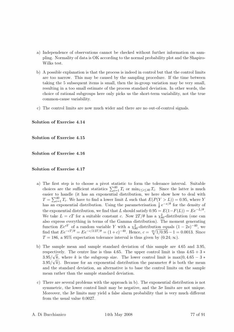
a) Independence of observations cannot be checked without further information on sam-pling. Normality of data is OK according to the normal probability plot and the Shapiro-Wilks test.

b) A possible explanation is that the process is indeed in control but that the control limitsare too narrow. This may be caused by the sampling procedure. If the time betweentaking the 5 subsequent items is small, then the in-group variation may be very small,resulting in a too small estimate of the process standard deviation. In other words, thechoice of rational subgroups here only picks us the short-term variability, not the truecommon-cause variability.

c) The control limits are now much wider and there are no out-of-control signals.





a) The first step is to choose a pivot statistic to form the tolerance interval. Suitablechoices are the sufficient statistics

∑40i=1 Ti or min1≤i≤40 Ti. Since the latter is much

easier to handle (it has an exponential distribution, we here show how to deal withT =

∑40i=1 Ti. We have to find a lower limit L such that E(P (Y > L)) = 0.95, where Y

has an exponential distribution. Using the parameterisation 1θ e−x/θ for the density of

the exponential distribution, we find that L should satisfy 0.95 = E(1−F (L)) = Ee−L/θ.We take L = cT for a suitable constant c. Now 2T/θ has a χ2

80-distribution (one canalso express everything in terms of the Gamma distribution). The moment generatingfunction EesY of a random variable Y with a χ2

80-distribution equals (1 − 2s)−40, wefind that Ee−cT/θ = Ee−c/2 2T/θ = (1+ c)−40. Hence, c = 40

√1/0.95− 1 = 0.0013. Since

T = 186, a 95% expectation tolerance interval is thus given by (0.24;∞).

b) The sample mean and sample standard deviation of this sample are 4.65 and 3.95,respectively. The centre line is thus 4.65. The upper control limit is thus 4.65 + 3 ∗3.95/

√k, where k is the subgroup size. The lower control limit is max(0, 4.65 − 3 ∗

3.95/√

k). Because for an exponential distribution the parameter θ is both the meanand the standard deviation, an alternative is to base the control limits on the samplemean rather than the sample standard deviation.

c) There are several problems with the approach in b). The exponential distribution is notsymmetric, the lower control limit may be negative, and the 3σ limits are not unique.Moreover, the 3σ limits may yield a false alarm probability that is very much differentfrom the usual value 0.0027.


d) The sequential likelihood ratio is given by

log Λn = n log5

3+

(1

5− 1

3

) n∑

i=1

Xi.

The corresponding lower CUSUM chart is given by

C−n = min

(0, C−

n−1 −(

1

5− 1

3

)Xn − log

5

3

).




Useful Results from Probability

Theory

In this appendix we present some useful results and notations from probability theory. Proofsof these results can be found in textbooks.

Theorem .0.1 (Markov inequality) Let X be a non-negative random variable. Then

P (X ≥ a) ≤ 1

aEX, a > 0.

Definition .0.2 Let Xn and Yn, n ∈ N, be random variables on the same probability space.We write

Xn = OP (Yn)

to mean that for each ε > 0, there exists an M ∈ R such that P (|Xn| ≥ M |Yn|) < ε, for nlarge enough. We write

Xn = oP (Yn)

to mean that P (|Xn| ≥ δ|Yn|)→ 0, for each δ > 0, as n→∞. Often these notations are usedfor deterministic Yn, or even for Yn = 1.

Lemma .0.3 Let Xn, Yn be m-dimensional random vectors and Wn k-dimensional randomvectors.

a) If Xnd−→ X and f : Rd → Rk is continuous, then f(Xn)

d−→ f(X).

b) If Xnd−→ X and Xn − Yn

P−→ 0, then Ynd−→ X.

c) If Xnd−→ X and Wn

d−→ c, then

(Xn

Wn

)d−→(

X

c

).

Remark .0.4 Part c) cannot be generalized by assuming Wnd−→ W . However, if Xn and

Wn are independent, then the result follows from the fact that in this case the joint distributionfunction factors. We use this in b) of the following corollary.

Corollary .0.5 Let Xn and Yn be m-dimensional random vectors defined on the same prob-ability space.

a) If Xnd−→ X and Yn

d−→ c, then Xn + Ynd−→ X + c .

79

b) If Xnd−→ X and Yn

d−→ Y and Xn and Yn are independent, then Xn + Yn convergesin law to the convolution of the distributions X and Y .

c) If Xnd−→ X and Yn

d−→ c, then Y Tn Xn

d−→ cT X.

Remark .0.6 Note that it does not necessarily hold in b) that the limit distribution equalsX + Y , since X and Y need not be independent or worse, need not be defined on the sameprobability space.

Lemma .0.7 Let Xn and Yn be d-dimensional random vectors.

a) If XnP−→ X and f : Rd → Rk is continuous, then f(Xn)

P−→ f(X).

b) If XnP−→ X and Xn − Yn

P−→ 0, then YnP−→ X.

c) If XnP−→ X and Wn are k-dimensional random vectors such that Wn

P−→ W , then(

Xn

Wn

)P−→(

X

W

).

Theorem .0.8 (Strong Law of Large Numbers) Let X, X1, X2, . . . be i.i.d. random vari-ables with common distribution function F and h : R→ R a function such that E |h(X)| <∞.Then

1

n

n∑

i=1

h(Xi)→ Eh(X) a.s. (n→∞).

Theorem .0.9 (Lindeberg Central Limit Theorem) Let Xn,1, . . . , Xn,rn be independentrandom variables for every n ∈ N with rn ∈ N. Assume EXn,k = 0 and σ2

n,k = VarXn,k <∞.

Set σ2n = Var

∑rnk=1 Xn,k =

∑rnk=1 σ2

n,k. If for all ε > 0

1

σ2n

rn∑

k=1

E(X2

n,k1[|Xn,k|>εσn]

)→ 0 (n→∞),

then1

σn

rn∑

k=1

Xn,kd−→ N(0, 1).

Theorem .0.10 (Multivariate central limit theorem) Let X1, . . . , Xn be i.i.d. randomvectors with existing covariance matrix Σ| . Then, as n→∞,

n12

(1

n

n∑

i=1

Xi − EX1

)d−→ N(〈0, . . . , 0〉, Σ| ).

For some distributions it is useful to know the basic properties of the Gamma function .This function is defined for positive x as

Γ(x) =

∫ ∞

0e−t tx−1 dt

Useful properties of the Gamma function are


• Γ(n + 1) = n! for non-negative integer n

• Γ(x + 1) = xΓ(x)

• Γ(12) =

√π

The second property also defines the Gamma function for negative, non-integer x.

Definition .0.11 (χ2-distribution) The χ2-distribution is characterised by one parameter,denoted here by n, and known as the “degrees of freedom”. Notation: χ2

n. The name of the χ2-distribution is derived from its relation to the standard normal distribution: if Z is a standardnormal random variable, then its square X = Z2 is χ2 distributed, with one degree of freedom.If Xi are χ2 distributed, and mutually independent, then the sum X =

∑i Xi is χ2 and the

parameter (degrees of freedom) is the sum of the parameters of the individual Xi. If X1, . . . , Xn

are independent random variables each with a N(µ, σ2) distribution, then the random variable(n−1)S2/σ2 has a χ2

n−1-distribution. The χ2-distribution is also a special case of the Gammadistribution, with α = ν/2 and λ = 1/2. The χ2-distribution is of great importance in theAnalysis of Variance (ANOVA), contingency table tests, and goodness-of-fit tests. The density

is given bye−x/2 x(ν−2)/2

2ν/2 Γ(ν/2).

Definition .0.12 ((Noncentral) t-distribution) Let Z be a standard normal random vari-able and let Y be a χ2-distributed random variable with ν degrees of freedom. If Z and Y areindependent, then the distribution of

Z + δ√Y

ν

is called a noncentral t-distribution with ν degrees of freedom and non-centrality parameter δ.The case δ = 0 is known as the (Student) t-distribution and has density

Γ

(n + 1

2

)

√nπ Γ

(n

2

)(1 +

x2

n

)(n+1)/2.

For a normal sample X1, . . . , Xn with mean µ and variance σ2,(X − µ

)/(S/

√n) has a Stu-

dent t-distribution with n − 1 degrees of freedom. The Student t-distribution is named afterthe statistician William Gosset. His employer, the Guinness breweries, prohibited any scien-tific publication by its employees. Hence, Gosset published using a pen name, Student. Forfurther properties and examples of the use of the noncentral t-distribution, we refer to Kotzand Johnson (1993) and Owen (1968).

Definition .0.13 (F -distribution) The F -distribution, named after the famous statisticianFisher, is the distribution of a ratio of two independent χ2 random variables. It has twoparameters, denoted by m and n, which are called the degrees of freedom of the numerator andthe denominator, respectively. Notation: Fm

n . If X is Student t-distributed with n degrees offreedom, then X2 is an F 1

n variable. If U is χ2 distributed with m degrees of freedom, V is

χ2 distributed with n degrees of freedom, and if U and V are independent, then X = U/mV/n is


an Fmn variable. The values fm

n;α are defined by P(Fm

n > fmn;α

)= α (so they do not follow the

customary definition of quantiles). From the definition of Fmn as a ratio of two χ2 variables,

it follows that fmn;1−α = 1/fn

m;α. The density is given by

Γ

(m + n

2

)

Γ(m

2

)Γ(n

2

) mm/2 nn/2 x(m/2)−1

(n + mx)(m+n)/2.

Definition .0.14 (Gamma distribution) Special cases of the Gamma distribution includethe χ2-distribution (α = ν/2 and λ = 1/2), the Erlang distribution (α positive integer) andthe exponential distribution (α = 1). Sometimes β = 1/λ is used as parameter. The density

is given by λα xα−1 e−λ x

Γ(α).


Index

ARL, 49ARLin, 49ARLout, 49B3, 49B4, 49D3(n), 48D4(n), 48LCL, 44UCL, 44Φ, 17∗, 26ϕ, 26c4(n), 23, 46d, 14d2(n), 47, 48

AMISE, 39attach, 8

bandwidth, 33biweight

kernel, 33Box, 4

capabilityratio, 14

capability indexlong-term, 17short-term, 17

causescommon, 3special, 3

Central Limit Theorem, 80chart

Pareto, 5χ2-distribution, 81chisq, 9CL, 44common causes, 3complete

family, 22

statistic, 22

control

in, 4

out-of, 4

control chart

R, 47

S, 49

S2, 48

X, 44

cuscore, 55

CUSUM, 54

EWMA, 57

GLR, 55

control limit

probabilistic, 48

convolution, 35

Cp, 14

Cpk, 14

CR, 14

cuscore chart, 55

CUSUM

FIR, 54

delta method, 25

Deming, 4

density, 33

detach, 8

distribution

χ2, 81

F -, 81

gamma, 82

dmo, 17

dpm, 17

Epanechnikov

kernel, 33

error

type I, 49

83

INDEX

type II, 49estimator

kernel, 33naive density, 32UMVU, 19

EWMA, 57exp, 9

Factorization Lemma, 20family

complete, 22Fast Fourier Transform, 36FFT, 36FIR, 54Fourier analysis, 35Function

Gamma, 80function, 10F -distribution, 81

Gammadistribution, 82function, 80

gamma, 9Gaussian

kernel, 33getwd(), 8GLR, 55

help.search, 8histogram, 31

in-control, 4induced likelihood function, 18inequality

Markov, 79invariance

MLE, 18Ishikawa, 4

Juran, 4

k, 17kernel

biweight, 33Epanechnikov, 33estimator, 33function, 32

Gaussian, 33Laplace, 42naive, 33rectangular, 33triangular, 33

ks.test, 9

Laplace kernel, 42LCL

R chart, 48S chart, 49

Lehmann-Scheffétheorem, 23

lemmafactorization, 20Slutsky, 79, 80

likelihood functioninduced, 18

limitwarning, 45

long-term capability index, 17LSL, 13

Markovinequality, 79

matrix, 8Maximum Likelihood

invariance, 18method

delta, 25MISE, 35

asymptotic, 39

naivekernel, 33

naive density estimator, 32Neyman, 20normal, 9normal probability plot, 9

out-of-control, 4

Pareto chart, 5Parseval’s identity, 42partition, 31Phase

I, 14, 43II, 44


INDEX

pnorm, 8probabilistic control limits, 48process capability index, 14

quantile, 19, 26

R control chart, 47Rao-Blackwell theorem, 21rational subgroups, 44rectangular

kernel, 33rule

runs, 45run length, 49runs rule, 45

S control chart, 49S2 control chart, 48setwd, 8shapiro.test, 9Shewhart, 4

Walter, 4short-term capability index, 17Six Sigma, 17SLLN, 80Slutsky

Lemma, 80lemma, 79

special causes, 3specification limit

lower, 13upper, 13

statisticcomplete, 22sufficient, 20

Strong Law of Large Numbers, 80subgroup

rational, 44sufficient statistic, 20

t, 9t-distribution

t-distributionnoncentral, 81

t-distribution, 81Taguchi, 4theorem

central limit, 80

Cramér, 25Lehmann-Scheffé, 23Rao-Blackwell, 21

toleranceinterval

guaranteed content, 27interval

β-expectation, 28limit

lower, 28upper, 28

triangularkernel, 33

type I error, 49type II error, 49

UCLR chart, 48S chart, 49

UMVU estimator, 19USL, 13

warning limits, 45weibull, 9

X control chart, 44


INDEX


Bibliography

V. Abel and E. Fuchs. On the run length of one-sided Cusum procedures in the change-pointcase. Meth. Oper. Res., 50:133–137, 1985.

J. Aitchison and I. Dunsmore. Statistical Prediction Analysis. Cambridge University Press,1975.

W. Albers and W.C.M. Kallenberg. Estimation in Shewhart control charts: effects and cor-rections. Metrika, 59(3):207–234, 2004a. ISSN 0026-1335.

W. Albers and W.C.M. Kallenberg. Are estimated control charts in control? Statistics, 38(1):67–79, 2004b. ISSN 0233-1888.

D.E. Barton. Unbiased estimation of a set of probabilities. Biometrika, 48:227–229, 1961.

A.H. Bowker and H.P. Goode. Sampling Inspection for Variables. McGraw-Hill, New York,1952.

D. Brook and D.A. Evans. An approach to the probability distribution of CUSUM run length.Biometrika, 59:539–550, 1972.

M.E. Calzada and S.M. Scariano. Reconciling the integral equation and Markov chain ap-proaches for computing EWMA average run lengths. Comm. Statistics Simul. Comput., 32(2):591–604, 2003.

S. Chakraborti. Run length, average run length and false alarm rate of Shewhart x-bar chart:Exact derivations by conditioning. Commun. Statist. Simul., 29:61–81, 2000.

C.W. Champ and W.H. Woodall. Exact results for Shewhart control chart with supplementaryruns rules. Technometrics, 29:393–401, 1987.

C.W. Champ and W.H. Woodall. Signal probabilities of runs rules supplementing a Shewhartcontrol chart. Comm. Statist. Simul. Comput., 26(4):1347–1360, 1997.

J.T. Chang and R.D. Fricker. Detecting when a monotically increasing mean has crossed athreshold. J. Qual. Technology, 31:217–234, 1999.

S.V. Crowder, D.M. Hawkins, M.R. Reynolds Jr., and E. Yashchin. Process control andstatistical inference. J. Qual. Technol., 29:134–139, 1997.

V. Czitrom and P.D. Spagon, editors. Statistical Case Studies for Industrial Process Improve-ment, 1997. American Statistical Association and SIAM.

87

BIBLIOGRAPHY

R.B. D’Agostino and M.A. Stephens, editors. Goodness-of-fit techniques. Marcel Dekker, NewYork, 1986.

P. Deheuvels. Estimation nonparametrique de la densité par histogrammes generalisés. Revuede Statistique Appliquée, 35:5–42, 1977.

A. Di Bucchianico, J.H.J. Einmahl, and N.A. Mushkudiani. Smallest nonparametric toleranceregions. Ann. Statist., 29(5):1320–1343, 2001.

R.J.M.M. Does and B.F. Schriever. Variables control chart limits and tests for special causes.Stat. Neerlandica, 46:229–245, 1992.

K.R. Eberhardt, R.W. Mee, and C.P. Reeve. Computing factors for exact two-sided tolerancelimits for a normal distribution. Communications in Statistics - Simulation and Computa-tion, 18:397–413, 1989.

N.R. Farnum and L.W. Stanton. Using counts to monitor a process mean. Journal of QualityTechnology, 18:22–28, 1986.

N.R. Farnum and L.W. Stanton. Narrow limit gauging: Go or No Go? Quality Engineering,3:293–307, 1991.

E. Fix and J.L. Hodges. Discriminatory analysis - nonparametric discrimination: consistencyproperties. International Statistical Reviews, 57:238–247, 1989.

J.L. Folks, D.A. Pierce, and C. Stewart. Estimating the fraction of acceptable product. Tech-nometrics, 7:43–50, 1965.

M.J. Fryer. Some errors associated with the non-parametric estimation of density functions.Journal of the Institute of Mathematics and its Applications, 18:371–380, 1976.

J.C. Fu, G. Schmueli, and Y.M. Chang. A unified Markov chain approach for computing therun length distribution in control charts with simple or compound rules. Statist. Probab.Letters, 65:457–466, 2003.

F.F. Gan and T.C. Chang. Computing average run lengths of exponential EWMA charts.Journal Of Quality Technology, 32:183–187, 2000.

B.K. Ghosh, M.R. Reynolds, and Y.V. Hui. Shewhart x-charts with estimated process vari-ance. Comm. Statist. Theory Methods, 10:1797–1822, 1981.

M.A. Girshick and H. Rubin. A Bayes approach to a quality control model. Ann. Math.Statistics, 23:114–125, 1952.

H. Gitlow, A. Oppenheim, and R. Oppenheim. Quality Management: Tools and Methods forImprovement. Irwin, second edition, 1989.

M.S. Gold. The geometric approximation to the Cusum run length. Biometrika, 76:725–733,1989.

G.K. Griffith. Statistical Process Control Methods. ASQC Quality Press, Milwaukee, 1996.


BIBLIOGRAPHY

W.C. Guenther. A note on the Minimum Variance Unbiased estimate of the fraction of anormal distribution below a specification limit. American Statistician, 25:18–20, 1971.

I. Guttman. Statistical Tolerance regions: Classical and Bayesian. Charles Griffin, London,1970.

D.M. Hawkins. Evaluation of average run lengths of cumulative sum charts for an arbitrarydata distribution. Communications in Statistics C: Simulation, 21(4):1001–1020, 1992.

D.M. Hawkins and D.H. Olwell. Cumulative Sum Charts and Charting for Quality Improve-ment. Springer, New York, 1998.

D.M. Hawkins, P. Qiu, and C.W. Kang. The changepoint model for statistical process control.J. Qual. Technol., 35(4):355–366, 2003.

M. Jílek. A bibliography of statistical tolerance regions. Mathematische Operationsforschungund Statistik - Series Statistics, 12(441–456), 1981.

M. Jílek and H. Ackermann. A bibliography of statistical tolerance regions II. Statistics, 20:165–172, 1989.

C.-H. Jun and M.S. Choi. Simulating the average run length for CUSUM schemes usingvariance reduction techniques. Commun. Statist. Simul., 22:877–887, 1993.

K.W. Kemp. The efficient use of quality control data. The Institute of Mathematics & itsApplications Monograph Series, 4. The Clarendon Press Oxford University Press, Oxford,2001.

R.S. Kenett and S. Zacks. Modern Industrial Statistics. Duxbury Press, 1998.

S. Kotz and N.L. Johnson. Process Capability Indices. Chapman & Hall, London, 1993.

S. Kotz and C.R. Lovelace. Process Capability Indices in Theory and Practice. Arnold, London,1998.

T.L. Lai. Sequential changepoint detection in quality control and dynamical systems. J. Roy.Statist. Soc. Ser. B, 57:613–658, 1995.

T.L. Lai. Sequential Analysis: Some classical problems and new challenges. Stat. Sinica, 11:303–350, 2001.

G.J. Liebermann and G.J. Resnikoff. Sampling plans for inspection by variables. J. Amer.Stat. Assoc., 50:457–469, 1955.

J.M. Lucas and R.B. Crosier. Fast initial response for CUSUM quality control schemes: Giveyour CUSUM a head start. Technometrics, 24:199–205, 1982.

J.S. Marron and M.P. Wand. Exact mean integrated squared error. Annals of Statistics, 20:712–736, 1992.

D.C. Montgomery. Introduction to Statistical Quality Control. Wiley, 4th edition, 2000.

D.B. Owen. A survey of properties and applications of the noncentral t-distribution. Techno-metrics, 10:445–478, 1968.


BIBLIOGRAPHY

E.S. Page. Continuous inspection schemes. Biometrika, 41:100–115, 1954.

A.C. Palm, R.N. Rodriguez, F.A. Spiring, and D.J. Wheeler. Some perspectives and challengesfor control chart methods. J. Qual. Technology, 29:122–127, 1997.

E. Parzen. On estimation of a probability density function and mode. Annals of MathematicalStatistics, 33:1065–1076, 1962.

J.K. Patel. Tolerance limits - a review. Communications in Statistics A - Theory and Methods,15:2719–2762, 1986.

E. Paulson. A note on control limits. Annals of Mathematical Statistics, 14:90–93, 1943.

L.P. Provost and C.L. Norman. Variation through the ages. Qual. Progress, 23(12):39–44,1990.

S.J. Qin. Statistical process monitoring: basics and beyond. J. Chemometrics, 17:480–502,2003.

S.W. Roberts. Control charts based on geometric moving averages. Technometrics, 1:239–250,1959.

R.N. Rodriguez. Recent developments in process capability analysis. J. Qual. Technol., 24(4):176–187, 1992.

M. Rosenblatt. Remarks on some nonparametric estimates of a density function. Annals ofMathematical Statistics, 27:827–837, 1956.

G.C. Runger and M.C. Testik. Control charts for monitoring fault signatures: Cuscore versusGLR. Quality Rel. Eng. Int., 19(4):387 – 396, 2003.

A.N. Shiryaev. On optimum methods in quickest detection problems. Theor. Prob. Appl., 8:22–46, 1963.

B.W. Silverman. Density Estimation for Statistics and Data Analysis. Chapman & Hall,London, 1986.

W.L. Stephens. Control by gauging. Journal of the Royal Statistical Society B, 10:54–108,1948.

Z. Stoumbos, M.R. Reynolds Jr., T.P. Ryan, and W.H. Woodall. The state of statisticalprocess control as we proceed into the 21st century. J. Amer. Stat. Assoc., 95:992–998,2000.

R.A. Tapia and J.R. Thompson. Nonparametric Probability Density Estimation. The JohnHopkins University Press, Baltimore, 1978.

M.P. Wand and M.C. Jones. Kernel Smoothing. Chapman & Hall, London, 1995.

Western Electric Company. Statistical Quality Control Handbook, 1956.

D.J. Wheeler. The variance of an estimator in variables sampling. Technometrics, 12:751–755,1970.


BIBLIOGRAPHY

S. S. Wilks. Determination of sample sizes for setting tolerance limits. Ann. Math. Statistics,12:91–96, 1941.

W.H. William. On the Markov chain approach to the two-sided CUSUM procedure. Techno-metrics, 26:41–46, 1984.

W.H. Woodall. Controversies and contradictions in statistical process control. J. Qual. Tech-nol., 32:341–378, 2000.

W.H. Woodall and D.C. Montgomery. Research issues and ideas in statistical process control.J. Qual. Technol., 31:376–386, 1999.

P.W. Zehna. Invariance of maximum likelihood estimation. Annals of Mathematical Statistics,37:744, 1966.


lecture notes 3tu course applied statistics

Documents