newton-x a package for newtonian dynamics
TRANSCRIPT

www.newtonx.org
NEWTON-X a package for Newtonian dynamics close to the crossing seam Documentation based on NEWTON-X version 1.4.1 (release September 17, 2013)

NEWTON-X: Newtonian dynamics close to the crossing seam
ii Return to Table of Contents

NEWTON-X: Newtonian dynamics close to the crossing seam
iii Return to Table of Contents
1 Table of contents
1 TABLE OF CONTENTS ................................................................................................................................ III 2 ABOUT NEWTON-X ................................................................................................................................ 1
2.1 General Information ............................................................................................................................ 1 2.2 Contact Information ............................................................................................................................. 1 2.3 What is new in this version .................................................................................................................. 1
3 MIXED QUANTUM-CLASSICAL DYNAMICS SIMULATIONS ........................................................................... 2 4 DEVELOPERS, COLLABORATORS AND CONTRIBUTORS .............................................................................. 4 5 HOW TO REFERENCE NEWTON-X ............................................................................................................ 5 6 QUICK START ............................................................................................................................................. 6
6.1 NEWTON-X Tutorial............................................................................................................................ 6 6.2 The NXINP tool .................................................................................................................................... 6 6.3 Initial conditions generation ................................................................................................................ 7 6.4 Dynamics Input .................................................................................................................................... 7
6.4.1 Adiabatic dynamics (dynamics on one surface) .......................................................................................... 7 6.4.2 Non-adiabatic dynamics (Surface hopping) ................................................................................................ 8 6.4.3 Mixed adiabatic and non-adiabatic dynamics ............................................................................................. 8
6.5 Creating the trajectory inputs .............................................................................................................. 8 6.6 Running the dynamics .......................................................................................................................... 9 6.7 Where are the results? ......................................................................................................................... 9 6.8 Overview of the file structure ............................................................................................................... 9
6.8.1 Dynamics simulations ................................................................................................................................. 9 7 CAPABILITIES .......................................................................................................................................... 11
7.1 General features ................................................................................................................................. 11 7.2 Overview of the available interfaces .................................................................................................. 12
8 HOW TO GET NEWTON-X ...................................................................................................................... 13 9 HOW TO INSTALL NEWTON-X ............................................................................................................... 14
9.1 Binary distribution ............................................................................................................................. 14 9.2 To install NEWTON-X you need ........................................................................................................ 14 9.3 To run NEWTON-X you need ............................................................................................................. 14 9.4 Installation procedure ........................................................................................................................ 14 9.5 Setup of third-party programs ............................................................................................................ 16 9.6 Verification of installation ................................................................................................................. 17 9.7 Compatibility between DALTON and NEWTON-X installations ....................................................... 17
10 INITIAL CONDITIONS GENERATION ........................................................................................................... 19 10.1 How to execute INITICOND ......................................................................................................... 19 10.2 Input parameters ........................................................................................................................... 19 10.3 What you need to execute .............................................................................................................. 23
10.3.1 Additional files ......................................................................................................................................... 23 10.3.2 The JOB_AD directory ............................................................................................................................. 24 10.3.3 Save files option ....................................................................................................................................... 25
10.4 Output ............................................................................................................................................ 25 10.5 Running in several computers ....................................................................................................... 26
11 TRAJECTORY-INPUT GENERATION, INITIAL CONDITIONS FOR MULTIPLE STATES, AND SPECTRA ............... 27 11.1 NXINP and options in the MAKEDIR.PL program ....................................................................... 27 11.2 Transition spectra ......................................................................................................................... 28 11.3 Initial conditions for multiple states .............................................................................................. 30 11.4 Managing several trajectories ....................................................................................................... 30 11.5 About energy restrictions .............................................................................................................. 31
12 DYNAMICS INPUTS ................................................................................................................................... 32 12.1 What is necessary to run ............................................................................................................... 32
12.1.1 control.dyn ................................................................................................................................................ 32 12.1.2 Geometry .................................................................................................................................................. 34 12.1.3 Velocity .................................................................................................................................................... 34

NEWTON-X: Newtonian dynamics close to the crossing seam
iv Return to Table of Contents
12.1.4 Freezing atoms .......................................................................................................................................... 35 12.1.5 Specific input for quantum-chemistry electronic-structure calculations ................................................... 35
12.1.5.1 Which electronic method to use ..................................................................................................... 35 12.1.5.2 Using analytical models ................................................................................................................. 35 12.1.5.3 COLUMBUS ................................................................................................................................. 37 12.1.5.4 TURBOMOLE ............................................................................................................................... 39 12.1.5.5 DFTB ............................................................................................................................................. 40 12.1.5.6 GAUSSIAN ................................................................................................................................... 40 12.1.5.7 TINKER ......................................................................................................................................... 44 12.1.5.8 DFTB+ ........................................................................................................................................... 45 12.1.5.9 GAMESS ....................................................................................................................................... 45 12.1.5.10 Hybrid Gradients (QM/MM) .......................................................................................................... 46
12.1.6 Thermostat control .................................................................................................................................... 49 12.1.7 Non-adiabatic dynamics control ............................................................................................................... 50 12.1.8 Time-derivative couplings ........................................................................................................................ 54 12.1.9 Wave function coefficients ....................................................................................................................... 54 12.1.10 Propagation of molecular orbitals ........................................................................................................ 55 12.1.11 Boundaries ........................................................................................................................................... 55 12.1.12 Stop conditions .................................................................................................................................... 55
12.2 How to execute NEWTON-X ......................................................................................................... 56 12.3 Output files .................................................................................................................................... 56 12.4 Restarting the job .......................................................................................................................... 57 12.5 Customized analysis ...................................................................................................................... 58
13 STATISTICAL ANALYSIS ........................................................................................................................... 59 13.1 What is needed to run .................................................................................................................... 59 13.2 How to execute ANALYSIS ............................................................................................................ 60 13.3 Output files .................................................................................................................................... 60
14 NORMAL MODE AND ESSENTIAL DYNAMICS ANALYSIS .......................................................................... 63 14.1 Normal mode analysis ................................................................................................................... 63
14.1.1 Input parameters ....................................................................................................................................... 63 14.1.2 Text Output ............................................................................................................................................... 64 14.1.3 Graphical Output ...................................................................................................................................... 64
14.2 Trajectory alignment ..................................................................................................................... 65 14.2.1 Input parameters ....................................................................................................................................... 65
14.3 Average Structure .......................................................................................................................... 65 14.3.1 Input parameters ....................................................................................................................................... 65
14.4 Essential Dynamics ....................................................................................................................... 66 14.4.1 Input parameters ....................................................................................................................................... 66
14.5 Python subroutine libraries ........................................................................................................... 66 14.6 Required packages to run NMA analysis ...................................................................................... 67
15 TOOLS ..................................................................................................................................................... 68 15.1 Plotting energy x time ................................................................................................................... 68 15.2 Plotting velocities and molecular orbitals..................................................................................... 68 15.3 Smoothangle .................................................................................................................................. 69 15.4 Collectjumps .................................................................................................................................. 69 15.5 Diagnostic ..................................................................................................................................... 70 15.6 Conversion tools ............................................................................................................................ 70 15.7 Split and merge initial conditions ................................................................................................. 71
16 TECHNICAL DETAILS ................................................................................................................................ 72 16.1 Templates and interfaces with new programs ............................................................................... 72 16.2 Conversion factors ........................................................................................................................ 73 16.3 Format of internal files ................................................................................................................. 73 16.4 Normal modes ............................................................................................................................... 74 16.5 Output files of the SH program ..................................................................................................... 75 16.6 CIOVERLAP documentation ......................................................................................................... 75
16.6.1 CIOVERLAP program ............................................................................................................................. 76 16.6.2 CIS_CASIDA ........................................................................................................................................... 77 16.6.3 CIS_SLATERGEN ................................................................................................................................... 78 16.6.4 CIVECCOMPARE ................................................................................................................................... 78 16.6.5 CIVECCONSOLIDATE .......................................................................................................................... 79 16.6.6 READSIFS ............................................................................................................................................... 80 16.6.7 CIPC.X, MCPC.X .................................................................................................................................... 80
16.7 Quick description of the programs ................................................................................................ 80 16.7.1 Initial conditions ....................................................................................................................................... 80 16.7.2 Dynamics .................................................................................................................................................. 81

NEWTON-X: Newtonian dynamics close to the crossing seam
v Return to Table of Contents
16.7.3 Tools ......................................................................................................................................................... 82 16.7.4 Statistical analysis ..................................................................................................................................... 82
17 LINKS TO THIRD-PARTY PROGRAMS ......................................................................................................... 84 18 REFERENCES ............................................................................................................................................ 85

NEWTON-X: Newtonian dynamics close to the crossing seam
1 Return to Table of Contents
2 About NEWTON-X
2.1 General Information
NEWTON-X1-3 is a general-purpose program for molecular dynamics in the electronic excited states, including non-adiabatic effects via surface hopping. NEWTON-X modular development allows it to be easily linked to any quantum chemistry package that can provide energy gradients and (optionally) nonadiabatic coupling vectors. In the current version, NEWTON-X can simulate nonadiabatic dynamics using COLUMBUS,4,5 TURBOMOLE,6 GAUSSIAN 03,7 GAUSSIAN 09,8 and GAMESS9 program packages. Adiabatic dynamics is also available with DFTB10 and DFTB+. Dynamics using hybrid gradients (including QM/MM approach) is available for combinations between TINKER11 and one of the following programs COLUMBUS, TURBOMOLE, DFTB+, and analytical models. Other third-party programs providing energies and nonadiabatic couplings can be easily integrated to work with NEWTON-X as well. NEWTON-X code is distributed free of charge for non-commercial and non-profit uses. You may use the program freely and adapt the code to your needs. Please, if you have any enhancements, share them with us. You are, however, not allowed to re-distribute code or binaries in parts or total. Anyone intending to use NEWTON-X must contact us. NEWTON-X is shipped to the user "as is". There is no guarantee that it will work as described. Usage is at your own risk, there is no liability taken for any damage or loss of data and/or money. If you experience problems please tell the developers supplying the version-number. They are always grateful for any hint, but bear in mind that there is no kind of official support for NEWTON-X.
2.2 Contact Information
Mario Barbatti Max-Planck-Institut für Kohlenforschung Kaiser-Wilhelm-Platz 1 D-45470 Mülheim an der Ruhr, Germany [email protected] www.barbatti.org The program, this documentation, and tutorials can be downloaded from: www.newtonx.org Support can be obtained through the discussion forum at: https://groups.google.com/forum/?fromgroups#!forum/newtonx
2.3 What is new in this version
NEWTON-X version 1.4.0 is a major update over version 1.3.1. The main modification is the inclusion of nonadiabatic dynamics at TDDFT level with GAUSSIAN 09 and at CC2 and ADC(2) levels with TURBOMOLE.
NEWTON-X: Newtonian dynamics close to the crossing seam
2 Return to Table of Contents
3 Mixed quantum-classical dynamics simulations
Mixed quantum-classical approaches12 are probably the most employed class of methods to perform excited-state molecular dynamics simulations including non-adiabatic effects. In these approaches, which include the surface hopping and the Ehrenfest methods, the nuclear time evolution is treated classically by means of the Newton’s equations, while the time evolution of the population of each electronic state is treated separately. In the surface hopping method,13 the time evolution of the population is obtained in two steps: first, non-adiabatic transition probability between each pair of states is computed and a stochastic algorithm is applied to decide in which state the classical trajectory is propagated in the next time step. Second, statistics over a large set of independently computed trajectories allows getting the fraction of trajectories (occupation) in each state as a function of time. The main hypothesis behind the surface hopping approach is that the occupation and the quantum population of each electronic state are the same if an infinite number of trajectories are computed.14 A recent review of the method is done in Ref.15.
There are several proposed ways to evaluate the non-adiabatic transition probabilities, since the most simple methods which just assume that the probability is the unity if the energy gap between the states is smaller than some threshold, to more sophisticated approaches which take into account the variation of wavefunction coefficients16 or compute the Landau-Zener transition probability.17 The most reliable procedure to compute the non-adiabatic transition probability for surface hopping simulations is the Tully’s fewest switches algorithm.14 In this approach, the time-dependent Schroedinger equation (TDSE) is integrated simultaneously to the classical trajectory.18 To cope with the lack of non-local information introduced by the on-the-fly approach, non-local terms in the TDSE are neglect and the nuclear wavefunction is supposed to be entirely localized at the classical position determined by the Newton’s equation. The integration of this semi-classical version of the TDSE gives the adiabatic populations of the electronic states, which are then used to compute the probability using the fewest-switches formula.
The integration of the TDSE depends on nonadiabatic coupling terms connecting different states. If adiabatic representation is used to expand the molecular wavefunction, non-adiabatic coupling vectors should be computed. Alternatively, if diabatic representation is used, non-diagonal Hamiltonian matrix elements should be computed. Either way, the computation of the non-adiabatic coupling terms are the bottleneck for non-adiabatic dynamics approaches. These terms are not usually available for most of quantum chemical methods and when they are, their computational cost increases with the square of the number of electronic states.19 These difficulties have motivated, on one hand, the search for approximated hopping algorithms as those mentioned above, and on the other hand the computation of the coupling terms based on wavefunction overlaps.16,19-23 Besides that, it has been an important achievement the development of procedures for analytical computation of them at the multireference configuration interaction (MRCI) and at the multiconfigurational self-consistent field (MCSCF) methods.24,25
One consequence of the hyperlocalization of the nuclear wavefunction in mixed quantum-classical approaches is that non-diagonal terms in the density matrix do not vanish with time as they should do.26,27 In surface-hopping, this lack of decoherence results in an excessive number of hopping events from lower to upper states, which disturbs the accomplishment of the occupation/population hypothesis mentioned above. Decoherence can be imposed by applying an ad hoc correction to the

NEWTON-X: Newtonian dynamics close to the crossing seam
3 Return to Table of Contents
adiabatic population every time step, which forces the non-diagonal terms in the density matrix to damp to zero within a certain time constant.27
When a hopping between two states takes place, it usually does through finite energy gap. In order to keep the total energy constant in the subsequent trajectory, it is necessary to correct the kinetic energy, for example, by rescaling the momentum or by adding more momentum at the direction of the non-adiabatic coupling vector.18,28 It may also happen that the stochastic algorithm attempts to make a hopping from a lower to an upper state in a region where there is not enough energy to do so. Such cases have been usually treated by forbidding the hopping occurrence.18 The momentum can be kept or reversed afterwards. Another possibility is to take the time uncertainty principle to search for a geometry nearby where the hopping is allowed.29
Because of the stochastic nature of the fewest-switches surface-hopping approach, trajectories starting with the same initial conditions will give rise to different time development. Moreover, the initial conditions should reflect the initial phase space distribution. Therefore the averages that define the state occupation should in principle be performed over this double ensemble of trajectories starting in different points of the phase space, several times in each one. Because of computational limitations, this procedure is usually reduced to a single ensemble of trajectories starting in different points of the phase space only once in each one.
The initial condition ensemble can be generated in a diversity of ways. For instance, the simulation of an instantaneously excited wave packet into the Franck-Condon region may be done by selecting geometries and velocities from a dynamics in the grounds state, regarding this dynamics run for long enough period as to allow an adequate sampling of the phase space. Alternatively, each nuclear degree of freedom can be treated within the harmonic approximation and a Wigner distribution can be build.
Most of the methods and algorithms mentioned in this short introduction are implemented in the NEWTON-X program.

NEWTON-X: Newtonian dynamics close to the crossing seam
4 Return to Table of Contents
4 Developers, Collaborators and Contributors
The NEWTON-X program has been developed in a multi-institutional collaboration, involving researchers from several countries. People working in the general NEWTON-X development are: Mario Barbatti Max-Planck-Institut für Kohlenforschung Germany Hans Lischka University of Vienna/Texas Tech Austria/USA Matthias Ruckenbauer University of Vienna Austria Felix Plasser University of Vienna Austria Many other people have contributed in the past or are still contributing to development of specific algorithms in NEWTON-X. They are: Surface hopping routines and initial condition distributions Giovanni Granucci University of Pisa Italy Maurizio Persico University of Pisa Italy Time-dependent non-adiabatic couplings Jiri Pittner J. Heyrovsky Institute Czech Republic NEWTON-X/GAMESS interface Aaron West Iowa State University USA Theresa Windus Iowa State University USA NEWTON-X/GAUSSIAN 09 interface Rachel Crespo-Otero University of Bath UK Contributions from the following colleagues are also acknowledged: Mirjana Eckert-Maksić, Sergio A. Losilla Fernández, Vladimir Lukeš, Peter Szalay, Bernhard Sellner, Atila Tajti, Mario Vazdar, Markus Weihs, Gunther Zechmann, Tomas Zeleny.

NEWTON-X: Newtonian dynamics close to the crossing seam
5 Return to Table of Contents
5 How to reference NEWTON-X
Please, cite NEWTON-X as:
• M. Barbatti, M. Ruckenbauer, F. Plasser, J. Pittner, G. Granucci, M. Persico, and H. Lischka, WIREs: Comp. Mol. Sci. 4, 26 (2014).
• M. Barbatti, G. Granucci, M. Persico, M. Ruckenbauer, M. Vazdar, M. Eckert-Maksić and H.
Lischka, J. Photochem. Photobio. A 190, 228 (2007).
• M. Barbatti, G. Granucci, M. Ruckenbauer, F. Plasser, R. Crespo-Otero, J. Pittner, M. Persico, H. Lischka, NEWTON-X: a package for Newtonian dynamics close to the crossing seam, version 1.4, www.newtonx.org (2013).
References to specific methods, algorithms and third-party programs used in NEWTON-X are given along this documentation. For a summary, see Chapter 7.

NEWTON-X: Newtonian dynamics close to the crossing seam
6 Return to Table of Contents
6 Quick start
6.1 NEWTON-X Tutorial
NEWTON-X tutorials with step-by-step procedures for several examples are available at www.newtonx.org
6.2 The NXINP tool
Most of NEWTON-X inputs are prepared with nxinp program. To execute nxinp, type: $NX/nxinp The first screen should looks like: ============================================================ NEWTON-X Newtonian dynamics close to the crossing seam www.newtonx.org ============================================================ MAIN MENU 1. GENERATE INITIAL CONDITIONS 2. SET BASIC INPUT 3. SET GENERAL OPTIONS 4. SET NON-ADIABATIC DYNAMICS 5. GENERATE TRAJECTORIES AND SPECTRUM 6. SET STATISTICAL ANALYSIS 7. EXIT Select one option (1-7):_
The next sections will guide you through each one of these options. By now, it is enough to note that nxinp is self-explaining. When you select one of the options, say, option 2 (Set basic input), you are asked about a series of parameters. A sequence of input may be, for example: ============================================================ NEWTON-X Newtonian dynamics close to the crossing seam www.newtonx.org ============================================================ SET BASIC OPTIONS nat: Number of atoms.

NEWTON-X: Newtonian dynamics close to the crossing seam
7 Return to Table of Contents
There is no value attributed to nat Enter the value of nat : 12 Setting nat = 12 nstat: Number of states. The current value of nstat is: 2 Enter the new value of nstat : 3 Setting nstat = 3 nstatdyn: Initial state (1 - ground state). The current value of nstatdyn is: 2 Enter the new value of nstatdyn : Setting nstatdyn = 2 dt: Time step for the classical equations. The current value of dt (fs) is: 0.5 Enter the new value of dt (fs) : 0.1 Setting dt = _
Each parameter contains a short description and, most of time, an attributed default value. To use the default values, just press <ENTER>. More information about each parameter can be found in this documentation.
6.3 Initial conditions generation
Input 1- Prepare geom file with equilibrium geometry. Use xyz2nx to create geom from xyz files. 2- Prepare force.out file with the harmonic frequencies using, for example, TURBOLOME. 3- Run nxinp program. Select option 1. GENERATE INITIAL CONDITIONS. nxinp will help you to
select the input parameters to control de initial condition generation. Exit nxinp. Run $NX/initcond.pl > initcond.log Output final_output: Initial conditions. initcond.log: Log file. Further options Optionally, you can control the number of excitation quanta in each vibrational modes by providing a file qvector (see Chapter 10) together with the other input files. It is also possible to pick points from previous dynamics calculations or to generate random velocities to be used as initial conditions.
6.4 Dynamics Input
6.4.1 Adiabatic dynamics (dynamics on one surface) Input
1- Create a directory called JOB_AD containing a set of input files for geometry optimization (1 step) with the chosen electronic structure program.
2- Run nxinp program. First, select option 2. SET BASIC INPUT. nxinp will help you to
select the input parameters to control the dynamics. After that, select option 3. SET
GENERAL OPTIONS if you want to change some more technical parameter. Exit nxinp. Hint Check control.dyn file. If the keyword “thres” is defined there, be sure that its value is 0 (thres = 0).

NEWTON-X: Newtonian dynamics close to the crossing seam
8 Return to Table of Contents
6.4.2 Non-adiabatic dynamics (Surface hopping) Input
1- Create a directory called JOB_NAD containing an input for non-adiabatic coupling (single point) with the chosen electronic structure program..
2- Run nxinp program ($NX/nxinp). First, select option 2. SET BASIC INPUT. nxinp will help
you to select the input parameters to control the dynamics. After that, select option 3. SET GENERAL OPTIONS if you want to change some more technical parameter. Optionally, select option 4. SET NON-ADIABATIC DYNAMICS to change the non-adiabatic-dynamics options. Exit nxinp.
Hint Check control.dyn file. If the keyword “thres” is defined there, be sure that its value is 100 (thres = 100).
6.4.3 Mixed adiabatic and non-adiabatic dynamics Input
1- Create a directory called JOB_AD containing a set of input files for geometry optimization (1 step) with the chosen electronic structure program.
2- Create a directory called JOB_NAD containing an input for non-adiabatic coupling (single
point).
3- Run nxinp program ($NX/nxinp). First, select option 2. SET BASIC INPUT. nxinp will help you to select the input parameters to control the dynamics. Optionally, select option 3. SET GENERAL OPTIONS if you want to change some more technical parameter. Optionally, select option 4. SET NON-ADIABATIC DYNAMICS to change the non-adiabatic-dynamics options. Exit nxinp.
Hint Check control.dyn file. The keyword “thres” must be defined there. Its value is the energy difference threshold (eV) bellow to which the non-adiabatic dynamics starts. This option is not fully tested.
6.5 Creating the trajectory inputs
Input 1- Copy final_output file created after the initial conditions generation, section 6.3, into the same
directory containing all files and directories created in the dynamics input, section 6.4. 2- If the jobs will run in a batch system, also copy the submission script file to that directory. In
$NX/../batch you may find several examples of submission scripts.
3- Run nxinp program ($NX/nxinp). Select option 5. GENERATE TRAJECTORIES AND SPECTRUM. nxinp will help you to select the input parameters to control the trajectory inputs generation. At the end of the input selection, NEWTON-X will automatically generate the trajectory directories. This process can take some few minutes.
Output

NEWTON-X: Newtonian dynamics close to the crossing seam
9 Return to Table of Contents
The trajectories inputs were written to TRAJECTORIES/TRAJn, where n is the trajectory number.
6.6 Running the dynamics
1- Go to each TRAJECTORIES/TRAJn (see section 6.5) and run $NX/moldyn.pl > moldyn.log & or, if is this the case, submit the job to the batch system.
2- Alternativelly, go to TRAJECTORIES and run $NX/submit.pl It will allow you to automatically submit several sequential jobs to the batch system.
6.7 Where are the results?
1- During or after the dynamics, go to directory TRAJECTORIES/TRAJn/RESULTS and run: $NX/plot to generate "energy x time" graph with GNUPLOT. molden dyn.mld to see motion with MOLDEN or any visualization package (xyz format). $NX/arrow to generate a MOLDEN file for a specific time step, containing the velocity and, in the case of dynamics with COLUMBUS, also molecular orbitals and non-adiabatic coupling vectors.
2- dyn.out file contains details about the geometry, velocity, energy and wave function
(adiabatic coefficients) along the trajectory. tprob contains information about the hopping probability at each time step. en.dat contains information about the energy of each state. sh.out contains further information about the TDSE integration.
3- In TRAJECTORIES/TRAJn, the standard output (moldyn.log) contains the log information of
the job and information about states, gradients and non-adiabatic couplings. The standard output is also written to RESULTS/nx.log.
4- In TRAJECTORIES/TRAJn/DEBUG, runnx.error contains occasional error messages. log.conv
contais the information about convergence of ab initio calculations.
5- TRAJECTORIES/TRAJn/INFO_RESTART contains a complete set of files to restart the dynamics from the last time step that run.
6.8 Overview of the file structure
6.8.1 Dynamics simulations The basic structure of directories and files during the dynamics simulations is shown in Figure 1. In the case of hybrid calculations (QM/MM) the structure is very similar. The main difference is that in this case the JOB_AD and JOB_NAD directories have a substructure specifying the several jobs. The inset in Figure 1 shows an example of this substructure for a QM/MM job with COLUMBUS and TINKER.

NEWTON-X: Newtonian dynamics close to the crossing seam
10 Return to Table of Contents
Figure 1 Basic structure of files and directories for a dynamics simulation. The inset shows an example for QM/MM simulations.

NEWTON-X: Newtonian dynamics close to the crossing seam
11 Return to Table of Contents
7 Capabilities
7.1 General features
Features Options Dynamics On-the-fly dynamics with the velocity-Verlet algorithm 30,31 Mixed quantum classical (nonadiabatic) dynamics 12
Surface hopping fewest switches algorithm14 Dynamics with non-adiabatic coupling vectors and time-derivative couplings19,20 Dynamics with Local Diabatization method21,32 Decoherence corrections27 Lagrangean extrapolation of orbitals33 Damped dynamics (kinetic energy always null) Andersen thermostat34,35 Hybrid dynamics (QM/MM)36
Interfaces COLUMBUS (MCSCF,MRCI)4,5 TURBOMOLE (TD-DFT, RI-CC2, ADC(2))6 DFTB (TD-DFTB)10 DFTB+ (DFTB) TINKER11 GAUSSIAN (CASSCF, TD-DFT)8 DFT-MRCI37 GAMESS (MCSCF, CCSD(T), MP2)9
Initial conditions Wigner distribution Quantum and classical harmonic oscillator distributions Pick points from previous dynamics Random velocity generation38
Spectrum simulation Photoabsorption cross section and photoemission spectra39
File management Friendly input via nxinp facility Automatic management of files and directories in multiple trajectories
Output and analysis Statistical analysis of results (internal coordinates and forces, energies, wave function
properties) Normal Mode Analysis, Essential Dynamics Analysis40,41 Recomputation of internal coordinates On-the-fly graphical outputs (MOLDEN, GNUPLOT)

NEWTON-X: Newtonian dynamics close to the crossing seam
12 Return to Table of Contents
7.2 Overview of the available interfaces
Initial conditions / Spectrum
Dynamics
Program
Version
Method
Frequency reading
Spectrum simulation
Adiabatic
Nonadiabatic (surface hopping)
NAC
CIO
LD
COLUMBUS 5.9 MRCI / MCSCF 7 MRCI / MCSCF TURBOMOLE TD-DFT CC2 / ADC(2) DFTB TD-DFTB DFTB+ DFTB GAUSSIAN 03 CASSCF 09 TDDFT TINKER MM DFT-MRCI DFT-MRCI GAMESS * MCSCF CCSD(T)/MP2 MOLDEN - ANALYTICAL User defined Available features NAC – Based on nonadiabatic coupling vectors. CIO – Based on wavefunction overlaps. LD – Based on local diabatization. * Initial conditions and adiabatic dynamics have been tested with GAMESS version 11 AUG 2011 (R1). Nonadiabatic jobs have been tested with a development version based on that version.

NEWTON-X: Newtonian dynamics close to the crossing seam
13 Return to Table of Contents
8 How to get NEWTON-X
NEWTON-X code is distributed free of charge for non-commercial and non-profit uses. To request a copy, visit www.newtonx.org. The third-party quantum chemistry and visualization programs are not distributed with NEWTON-X. They should be directly obtained from the respective distributors and owners.

NEWTON-X: Newtonian dynamics close to the crossing seam
14 Return to Table of Contents
9 How to install NEWTON-X
9.1 Binary distribution
Binary files for a Linux-compiled NEWTON-X are distributed together with the source code. As first option, we strongly recommend to use this version. In this case, just uncompress the distribution file tar –zxf nx-<version>.tgz or, alternatively, gunzip nx-<version>.tgz tar –xf nx-<version>.tar Then, set the shell-variable $NX to <install-path>/bin For c-shell users, this is done by: setenv NX <install-path>/bin For bash-shell users, this is done by: export NX=<install-path>/bin
9.2 To install NEWTON-X you need
We strongly recommend that you use the binary files that we provide. But if for any reason you wish to compile the program yourself, you will need: • The NEWTON-X source code. See Chapter 8 to see how to get the NEWTON-X source code. • A FORTRAN 90 compiler installed, preferentially the Intel Fortran compiler. • PERL 5.8.0 or higher installed (www.perl.com). • BLAS, LAPACK, and GSL libraries installed. More information on how to set the paths to these libraries can be found in the README.install file, which can be found in the NEWTON-X distribution.
9.3 To run NEWTON-X you need
• At least one of the interfaced third-party programs (COLUMBUS, TURBOMOLE, DFTB, TINKER, GAUSSIAN, GAMESS). See Chapter 7 of this documentation for an updated list of available interfaces. For the full functionality, you also need: • GNUPLOT (www.gnuplot.info). • Some molecular visualization program able to read xyz files (e.g., MOLDEN or VMD).
9.4 Installation procedure
Untar and uncompress the source code file tar –zxf nx-<version>.tgz or, alternatively, gunzip nx-<version>.tgz

NEWTON-X: Newtonian dynamics close to the crossing seam
15 Return to Table of Contents
tar –xf nx-<version>.tar The files will be written to the NX-pack directory. Go to the NX-pack/install subdirectory and run the script ./installnx.pl It will ask you for an installation address and for which packages you want to install. If the installation proceeds without problem, you will get in the screen something like: ================================================ Welcome to the NEWTON-X installation routine www.newtonx.org ================================================ Please enter directory for the NEWTON-X installation /home/users/NX ! Give the path in your system This directory seems not to exist - create it? (y/n) y Created directory /home/users/NX Select packages to be installed. [0] Complete installation [Default option] [1] Copy files and install tools (TOOLS) [2] Initial conditions (TOOLS+INITCOND) [3] Molecular dynamics (TOOLS+MOLDYN+MODEL) [4] Time-dependent overlaps (TOOLS+CIOVERLAP) Enter comma separated list or dash separated range: 0 ! Complete installation Starting NEWTON-X installation at Mon May 17 09:27:16 CEST 2010 Compiler keyword: ifort Flag keyword: -static -vec-report0 Program version: 1.2.0a (01/Jun/2010) Fortran version: /opt/intel/Compiler/11.1/069/bin/intel64/ifort Perl version: /usr/bin/perl Original directory: /home/users/NX-pack/install Installation directory: /home/users/NX BLAS: /opt/intel/mkl/10.1.3.027/lib/em64t/ GCC for LA libraries: /usr/bin/g++ GCC for cioverlap: /usr/bin/g++ BLAS for cioverlap: /usr/lib64 LAPACK for cioverlap: /usr/lib64 GSL for cioverlap: /usr/lib64 GSLCBLAS for cioverlap: /usr/lib64 Packages selected: 1 TOOLS 2 INITCOND 3 MOLDYN 4 CIOVERLAP Checking compilers, libraries and dependencies... No problem detected for the selected packages. Copying file .......................................................................... ..........................DONE Compiling INITCOND ........................DONE Compiling MOLDYN ................................................................DONE Compiling TOOLS ................................DONE Compiling MODEL ............DONE Compiling CIOVERLAP ................................DONE Setting permissions ........DONE Installation completed! Don't forget to set the environment variable $NX to /home/users/NX/bin
Do not forget to set the shell-variable $NX to <install-path>/bin after installation. For c-shell users, this is done by: setenv NX <install-path>/bin For bash-shell users, this is done by: export NX=<install-path>/bin

NEWTON-X: Newtonian dynamics close to the crossing seam
16 Return to Table of Contents
A complete installation log is written to installnx.log file. As default, instalnx.pl is set to use the Intel Fortran Compiler for Linux. To change the compiler and the compiler options follow the instructions contained in the installnx.pl body. More information on compilers can be found in the README.install file, which can be found in the NEWTON-X distribution. NEWTON-X has been compiled and tested in 32-bit, EM64T, and Opteron machines.
9.5 Setup of third-party programs
NEWTON-X works using third-party programs, such as COLUMBUS, TURBOMOLE, GAUSSIAN, and others. These programs should be separately obtained from their distributors and installed according to their specific instructions. Depending on the job, NEWTON-X assumes that a series of variables are defined in the system. They are:

NEWTON-X: Newtonian dynamics close to the crossing seam
17 Return to Table of Contents
Program Variable Example of file pointed by each variable COLUMBUS $COLUMBUS ls $COLUMBUS > ... runc ...
DFTB $DFTB ls $DFTB > ... dftb ....
DFTB+ $DFTPLUS ls $DFTBPLUS > dftb+
GAUSSIAN 03 $g03root ls $g03root/g03 > ... g03 ...
GAUSSIAN 091 $g09root ls $g09root/g09 > ... g09 ...
DFT-MRCI $DFTCI ls $DFTCI > ... mrci ...
$KSCIHOME ls $KSCIHOME > ... dftparam.s.bhlyp ...
GAMESS $GAMESS ls $GAMESS > ... rungms ...
TURBOMOLE2 $TURBODIR ls $TURBODIR > ... scripts bin ...
$PATH echo $PATH > ... :$TURBODIR/bin/x86_64-unknown-linux-gnu:$TURBODIR/scripts: ...
TINKER3 $PATH echo $PATH > ...:/usr/bin/tinker-bin-linux:...
1 In the case of GAUSSIAN 09, the GAUSSIAN profile must be sourced before executing NEWTON-X. Example (C-shell): source $g09root/g09/bsd/g09.login 2 For TURBOMOLE, directories containing the executables (e.g., $TURBODIR/bin/x86_64-unknown-linux-gnu) and scripts (e.g., $TURBODIR/scripts) must be in the standard path. 3 For TINKER, directories containing the executables (e.g., /usr/bin/tinker-bin-linux) must be in the standard path.
9.6 Verification of installation
To test the installation, create a directory to execute the tests. Move into it and select the tests that you want to perform by running $NX/inp-testnx.pl It will return a list of all available tests. You can select particular tests or all of them. It will create a file called test.inp containing a space-separated list with the number of the tests that should run. Then, run the program $NX/test-nx.pl > test-nx.log & This program will run the selected tests. If test.inp is not present, all tests are selected by default. The tests are a series of quick pre-build examples. It will check whether they have normal termination or not, and it will compare the results to those of standard files. Check the results in test-nx.log. Tests invoking GAMESS may need special adjustments for each system. When such tests are requested, inp-testnx.pl asks additionally a few questions about GAMESS environment (executable number, scratch directory, and execution script name). This information is written to games.par file, which is used by the jobs running under test-nx.pl command.
9.7 Compatibility between DALTON and NEWTON-X installations
Even after a successful installation, NEWTON-X jobs using COLUMBUS may return the following error message: readsifs returned with error! Are the integer formats between Columbus and NX matching? In such cases, the probable cause is an incompatibility issue between DALTON program (used by COLUMBUS) and NEWTON-X. It can be solved by recompiling CIOVERLAP program, by the following these steps:
1. Go to install directory. 2. Edit installnx.pl file and change the value of variable $status_record32. The default
value is “on” (SIFS integer format = 64 bits), which means that DALTON is assumed to have been compiled for 64 bits. “off” (SIFS integer format = 32 bits) means that DALTON is assumed to have been compiled for 32 bits.

NEWTON-X: Newtonian dynamics close to the crossing seam
18 Return to Table of Contents
3. Run the installation program again, but this time select option [4] Time-dependent overlaps (TOOLS+CIOVERLAP).
4. It is not necessary to recompile LA library. A previous installation of the LA library already exits. Do you want to replace it? (y/n) n

NEWTON-X: Newtonian dynamics close to the crossing seam
19 Return to Table of Contents
10 Initial conditions generation
INITCOND is a set of programs developed to generate initial conditions to the molecular dynamics and spectrum simulation. It is possible to generate initial conditions by sampling the data according to harmonic oscillator distributions (classical and quantum). It is also possible to pick at random points from a previous dynamics calculation performed with NEWTON-X or to generate random velocities for some specific geometry. For NACT = 1, 2 or 3 the initial conditions are based on normal modes. The normal modes themselves should be generated in a separated run and given as input to NEWTON-X. NEWTON-X can read the normal modes directly from the output files of several third-party programs (see IPROG below). Despite the initial format, the normal modes are internally transformed into mass-weighted normal modes L. For NACT = 1 or 2, for each normal mode, an amplitude nQ and a momentum nQ are randomly selected from a harmonic oscillator distribution. The Cartesian coordinates and velocities of all atoms are then determined from the normal coordinates by the inverse transformation.41 If NACT = 3, only nQ is randomly selected, while nQ is scaled as to give the harmonic oscillator energy. For NACT = 2, if the vibrational numbers are zero, the distributions matches the Wigner distribution for the quantum harmonic oscillator 42,43. For higher vibrational quantum numbers, the distribution for each normal mode is
( ) ( )22
nnNnN PQn
ξψ ,
where ( )nN Qn
ψ and ( )nn Pξ are respectively the harmonic oscillator wavefunctions in the coordinate and momentum spaces. If NACT = 4, random points are picked from a previously performed dynamics. If NACT = 5, random velocities are generated for a fixed velocity according to the algorithm described in Ref. 38. If NACT = 6, single point electronic structure calculations are performed for a previously computed set of initial conditions.
10.1 How to execute INITICOND
Run $NX/initcond.pl > initcond.log
10.2 Input parameters
File: initqp_input Namelist: DAT Parameter Default Description NUMAT = [3] number of atoms

NEWTON-X: Newtonian dynamics close to the crossing seam
20 Return to Table of Contents
NPOINTS = [1] number of initial conditions generated
NACT
= [2] 1 - Each normal mode contains a given energy in the initial state, according to the vibrational quantum number, and the distribution of coordinates and momenta is that of a classical harmonic oscillator. 2 - The distribution of coordinates and momenta is that of a quantum mechanical harmonic oscillator in the specified vibrational state. The sample of the coordinates and momenta is uncorrelated. In the ground vibrational state, this distribution matches the Wigner distribution for the harmonic oscillator. 3 - The distribution of coordinates and momenta is that of a quantum mechanical harmonic oscillator in the specified vibrational state. Only coordinates are sampled. For each normal mode, the momenta are scaled to the coordinates up to the have the correct harmonic vibrational energy. 4 - NPOINTS points are picked up from some previously run dynamics simulations. 5 - Gaussian-distributed random velocities are generated for some specific geometry. 6 - Single point electronic structure calculations for a previously computed set of initial conditions.
ISEED = [1] Random number seed 0 Use standard value for the random number seed. -1 Use random seed. Any interger > 0 is used as the seed itself. Use ISEED = -1 if the job will be split (see section 15.7).
LVPRT = [1] 1 - Standard print level. 2 - Debug print level.
If NACT ≤ 4 N_PICK = [-1] Method to pick up points:
-1 - pick random points from trajectories. n (integer) - pick time step n from trajectories.
NIS
= [1] Intial state (Ground state = 1).
NFS
= [2] Final state. (Information for all states between NIS and NFS are stored.)
CHK_E
= [0] 0 - Do not check the energies. 1 - Check the energies between states NIS and NFS. For ground state dynamics, set CHK_E = 0.
CMP_E = [0] (Only if NACT = 4 and CHK_E = 1) 0 - Read energies from dynamics output 1 - Compute energies.
PROG
= [1.0] (Only if CHK_E = 1 and NACT = 3 or CMP_E = 1 and NACT = 4) Program to compute vertical excitation energies: 1.0 - COLUMBUS 2.0 - TURBOMOLE RI-CC2 / ADC(2) 2.1 - TURBOMOLE TD-DFT 5.0 - DFTB 9.0 - DFT-MRCI 10.0 - GAMESS (MCSCF) 10.1 - GAMESS (other methods)
EVERT = [5.0] Required vertical energy (eV).
DE
= [0.5] Allowed variation EVERT (eV).
If NACT ≤ 3

NEWTON-X: Newtonian dynamics close to the crossing seam
21 Return to Table of Contents
FILE_GEOM = [geom] file containing the equilibrium geometry of the molecule in COLUMBUS and NEWTON-X format. (See section 15.6 for conversion tools)
FILE_NMODES = [nmodes] file containing the normal coordinates and the vibrational frequencies (in cm-1). Normally it is an output file from some quantum chemistry program (see option IPROG).
FILE_OUT = [ini_qv] output file from INIQP, containing NPOINTS set of generated Q and V.
FILE_VIB = [qvector] file with the vibrational quantum numbers. See description bellow.
ANH_F = [1.0] Multiply all frequencies by ANH_F. Useful to add anharmonic effects.
KVERT = [1] 0 - Use the provided EVERT. 1 - Use EVERT of the equilibrium geometry that is calculated in the first step of the program.
IPROG
= [1] Read vibrational modes from: 1 - GAMESS 2 - TURBOMOLE 3 - COLUMBUS 4 - GAUSSIAN 5 - MOLDEN 6 - DFTB 7 - ACES2
NM_FLAG = [0]
(Only if IPROG = 5) If normal modes should be read from a MOLDEN file, then the type of normal mode should be given. 1 - Cartesian normal modes (amu-1/2) 2 - Normalized Cartesian normal modes 3 - Mass weighted normal modes The default 0 will terminate the program.
IF NACT = 4 ADDRESS = [] Path to the set of previous trajectories from which the initial conditions must
be picked. The default address [/home/old_dyn/TRAJECTORIES] certainly should be changed.
TRAJI = [1] Initial trajectory to be read.
TRAJF = [10] Final trajectory to be read.
TI = [0] (Only if N_PICK = -1) Start to pick points only after time TI (fs) of each trajectory.
TF = [-1] (Only if N_PICK = -1) Do not pick points after time TF (fs) of each trajectory. Diagnostic.pl (see section 15.5) is always called in this kind of run. The time suggested in its output (diag.log) is used if it is smaller than TF. If TF = -1, always use the time suggested in diag.log file.
REORDER = [1] (Only if N_PICK = -1) Sort the points according to the trajectory number and time step. 0 - Do not sort. 1 -Sort.
ETOT_DEV = [0.5] Allowed variation in the total energy (eV).
POP_DEV = [0.1] Allowed variation in the norm of the adiabatic population.
IF NACT = 5 FILE_GEOM = [geom] file containing the initial geometry of the molecule in the COLUMBUS and
NEWTON-X format. (See section 15.6 for conversion tools)
EKIN = [0] Kinetic energy (eV).

NEWTON-X: Newtonian dynamics close to the crossing seam
22 Return to Table of Contents
TEMP = [0] Temperature (K). If TEMP = 0 (default), this option generates random velocities corresponding to kinetic energy Ekin (microcanonical ensemble). If TEMP > 0, canonical ensemble of random velocities is generated with mean kinetic energy EKIN and standard deviation σ = kBT(3N/2)1/2. In any case, translational and rotational velocities are zero.
IF NACT = 6 NIS
= [1] Intial state (Ground state = 1).
NFS
= [2] Final state. (Information for all states between NIS and NFS are stored.)
PROG
= [1.0] Program to compute vertical excitation energies: 1.0 - COLUMBUS 2.0 - TURBOMOLE RI-CC2 / ADC(2) 2.1 - TURBOMOLE TD-DFT 5.0 - DFTB 6.5 - GAUSSIAN 09 9.0 - DFT-MRCI 10.0 - GAMESS (MCSCF) 10.1 - GAMESS (other methods) 20 - Hybrid energies (QM/MM)
Example of initqp_input file: &DAT nact= 2, numat= 2, npoints= 20, file_geom= hf.geom, file_nmodes=hf.nmodes, file_out= qvector, evert= 5.0, de= 0.25, kvert= 1, chk_e= 1, prog = 1.0, iprog = 2.0, nis = 1, nfs = 2, &END File : columbus.par Optional file containing information for COLUMBUS jobs. Parameter Default Description MEM [200] COLUMBUS core memory in Mwords (1 GB = 134 Mwords). For
COLUMBUS 7, MEM is internally converted to GB.
File : turbomole.par Optional file containing information for TURBOMOLE jobs. Parameter Default Description PARALLEL [1] Number of cores to use for parallel Turbomole (SMP only, no MPI!)
File : dftb.par Optional file containing information for DFTB jobs. Parameter Default Description DFTB_EXEC = [dftb] Name of the DFTB executable file. $DFTB variable must be defined
in the system. NEWTON-X will run $DFTB/<dftb_exec>.
File : dftb+.par

NEWTON-X: Newtonian dynamics close to the crossing seam
23 Return to Table of Contents
Optional file containing information for DFTB+ jobs. Parameter Default Description DFTBP_EXEC = [dftb+] Name of the DFTB+ executable file. $DFTBPLUS variable must be
defined in the system. NEWTON-X will run $DFTBPLUS/<dftb_exec>.
File : dftci.par Optional file containing information for DFT-MRCI jobs. Parameter Default Description maxiter = [6] Maximum number of MRCI cycles.
File: gamess.par Parameter Default Description VERNO = [00] Version number of GAMESS executable.
NCPUS = 1 Number of computer processes to be run.
RUN_GAMESS = [rungms] Name of GAMESS execution script.
SCR
= [1] GAMESS scratch directory: 0: Use default GAMESS options as defined in RUN_GAMESS script. 1: Create SCR directory inside TEMP directory of NEWTON-X.
10.3 What you need to execute
• initqp_input with the set of parameters. (It can be generated with nxinp tool.)
10.3.1 Additional files If NACT ≤ 3:
• file with the equilibrium geometry (see FILE_GEOM keyword). Hint: the program tm2nx
converts the coord file (TURBOMOLE format) to the NEWTON-X format.
• file with the vibrational modes (see FILE_NMODES keyword). Warning 1: The atom order in FILENMODES and in FILE_GEOM must be the same. Warning 2: The orientation of the normal mode coordinates in FILENMODES orientation must be consistent with the orientation of the optimized geometry in FILE_GEOM.
• file with the vibrational quantum numbers (see FILE_VIB keyword). The default is the ground
state (0 quantum in each mode). If you want to change this default values, write to FILE_VIB a list of quanta in each mode. Example:
0 0 0 0 0 0 0 0 0 0 0 1
This example puts one quantum at the highest frequency mode of a system with 12 modes (6 atoms). Keep the format with 5 columns of integers. The order of the modes is the same as in FILE_NMODE. If FILE_VIB des not exist, the program assumes 0 for all modes. To set -0.5 for a mode makes this mode contribute with 0 to the initial energy.
• JOB_AD directory containing input files for excited-state single point calculation with a third-
party quantum chemistry program (only if CHK_E=1).
• save_file, optional file (see section 10.3.3).

NEWTON-X: Newtonian dynamics close to the crossing seam
24 Return to Table of Contents
If NACT = 4:
• The TRAJn directories of some dynamics calculations previously performed.
If NACT = 5:
• Geometry file with the initial geometry in NEWTON-X format. If NACT = 6:
• A previously computed set of initial conditions in the NEWTON-X format renamed
final_output.old. • JOB_AD directory containing input files for excited-state single point calculation with a third-
party quantum chemistry program.
• save_file, optional file (see section 10.3.3).
10.3.2 The JOB_AD directory The JOB_AD directory contains input files for excited-state single point calculation with a third-party quantum chemistry program. For the cases that this directory is needed, set the oscillator strength to be calculated by the quantum chemistry program. This will give you the possibility of generating UV spectra as well as to use the transition probability to select the initial conditions. Specifically for COLUMBUS calculations (PROG = 1.0): Input files must be prepared for a single point MCSCF or CI calculation in C1 point group (no symmetry). For DFTB calculations (PROG = 5.0): Input files must be prepared for excited-state spectrum calculation using code 10. The DFTB input parameter and geometry files must be named dftb.in and in.gen, respectively. For Gaussian 09 (PROG = 6.5): Prepare input files for a single point vertical excitation at the TDDFT level. The input file must be called gaussian.com and the geometry must be given in Cartesian coordinates. The check point file named gaussian.chk containing the initial molecular orbitals may be provided as well. A suitable example of gaussian.com content is: %chk=gaussian %mem=2000MB # B3LYP/6-31G(d) TD=NStates=2 NoSymm methaniminium 1 1 N 0.000000 0.000000 0.637342 C 0.000000 0.000000 -0.703614 H -0.648747 0.572349 1.177883 H 0.648745 -0.572350 1.177883 H 0.618844 0.701080 -1.278050 H -0.618844 -0.701080 -1.278049 Note that the geometry is given in Angstroms in this version of NEWTON-X. Up to NEWTON-X 1.3, the keyword Unit=AU was mandatory. To avoid troubles with differences between input and standard

NEWTON-X: Newtonian dynamics close to the crossing seam
25 Return to Table of Contents
orientations in Gaussian, it is highly recommended to use NoSymm keyword in the Gaussian.com as well as in the computation of the normal modes (FILE_NMODES). NEWTON-X executes GAUSSIAN 09 by invoking the command: g09 < gaussian.com It is assumed that the user sources the g09 profile before running NEWTON-X. For DFTB+ calculations (PROG = 8.0): Input files must be prepared for a DFTB calculations yielding energy and gradient. The DFTB input parameter and geometry files must be named dftb.in and in.gen, respectively. At the present, only ground state dynamics (no TD) is available with this program. For DFT-MRCI calculations (PROG = 9.0): JOB_AD should contain a complete set of input files for TURBOMOLE DFT calculation, including the auxiliary basis set, and the specific input file for the DFT-MRCI program. The DFT-MRCI input file must be named mrci.inp and should be set to the total number of excited states.
10.3.3 Save files option When electronic structure calculations are performed during the initial condition generation (NACT ≤ 3 with CHK_E = 1 or NACT = 6), it is possible to give a list of files or directories that should be saved for every initial condition. This is simply done by creating a file name save_file and including a list of file names to be saved. save_file must contain only one file name per line. For instance, you may want to save the molecular orbitals (mos file) and the scf log file (dscf.out) resulting from the TURBOMOLE calculations for each initial condition. In this case the following save_file should be given together with the other input files: Example of save_file file: dscf.out mos The required files are tar-compressed and written to the DEBUG directory renamed as ic<card>-filename.tgz, where <card> is the number of the initial condition as given in the final_output file. For the example above, DEBUG will contain: ic0-dscf.out.tgz ic0-mos.tgz ic1-dscf.out.tgz ic1-mos.tgz ic2-dscf.out.tgz ic2-mos.tgz … ic0-<NPOINTS>.out.tgz ic0-<NPOINTS>.tgz The routine that saves the files runs right after the execution of the third-party program, before the cleanup of execution directory. If the file that should be saved is inside a directory, the relative path must be provided. For instance, if we want to save the MCSCF log file of COLUMBUS jobs (mcscfsm.sp), save_file should contain “LISTINGS/mcscfsm.sp”. The full LISTINGS directory will be saved is save_file contains “LISTINGS”.
10.4 Output
The initial conditions are written to final_output file. The data from spectrum simulation are written to the cross-section.dat, spectrum.dat and spectrum-hist.dat files.

NEWTON-X: Newtonian dynamics close to the crossing seam
26 Return to Table of Contents
Initial condition for multiple states are written to final_output.[initial-state].[final-state]. Thus, for example, final_output.1.3 contains initial conditions for transitions from state 1 (ground state) to state 3. The final_output file is the same as final_output.[NIS].[NFS]. DEBUG directory contains the error log information (runnx.error) and files that should be saved when save_file file is provided (see section 10.3.3).
10.5 Running in several computers
It is possible to split the spectrum and initial condition generation job to run in different computers and merge them again afterwards. See section 15.7 for general instructions. Do not forget to set ISEED = -1 when the jobs are split.

NEWTON-X: Newtonian dynamics close to the crossing seam
27 Return to Table of Contents
11 Trajectory-input generation, initial conditions for multiple states, and spectra
11.1 NXINP and options in the MAKEDIR.PL program
The section “5. GENERATE TRAJECTORIES AND SPECTRUM” of nxinp input program allows multiple different tasks, which can be selected in the sub menu: ============================================================ NEWTON-X Newtonian dynamics close to the crossing seam www.newtonx.org ============================================================ GENERATE TRAJECTORIES AND SPECTRUM type: What do you want to do? 1 - Generate spectrum 2 - Select initial conditions for multiple initial states 3 - Generate trajectories 4 - Return to main menu The current value of type is: 3 Enter the new value of type : After selecting one of these options, you will be asked a series of question about the specificities of your job. At the end, the file mkd.inp will be generated and the program makedir.pl will be automatically running when you see the message: Processing data: This may take some minutes. Please, wait... If you want, after leaving nxinp, makedir.pl can be executed again by running: $NX/makedir.pl > makedir.log The options in makedir.pl may be changed by setting the following keywords in mkd.inp. Name: mkd.inp Parameter Default Description TYPE = [3] 1 - Generate spectrum
2 - Select initial conditions for multiple initial states 3 - Generate trajectories
NIS = [1] Initial state. 1 is the ground state. (Spectrum simulation.)
NFS = [2] Array of final states (space separated, e.g., 2 3 4). If not only spectrum, but trajectories input is required as well, only one final state is allowed.
SCREEN = [0] Energy restriction:

NEWTON-X: Newtonian dynamics close to the crossing seam
28 Return to Table of Contents
0 - don't apply any restriction 1 - use the original energy restriction written in the final_output files 2 - apply new energy restriction
E_CENTER = [0.0] Center of the energy restriction (Only if SCREEN = 2) x - value of the center of restriction (eV) ref n - use the vertical excitation of final_output.nis.n file
E_VAR = [0.5] Width of the energy restriction. (eV) (Only if SCREEN = 2)
OS_CONDON = [-1] Oscillator strength: -1 - try to read from final_output file x - oscillator strength is always x (Condon approximation)
PROB_KIND = [F] Probabilities in the spectrum generation will be computed according to A – Einstein-coefficients A (spontaneous emission) B – Einstein-coefficients B (induced absorption or induced emission) E – Fluorescence (radiative decay rate) F – Absorption (photoabsorption cross section)
NORM = [local] Normalization of the Eintein's coefficients: local - Use energy-restricted data set global - Use complete data set
SEED = [0] Seed for the random number generation 0 - a default random number seed is used 1 - a randomized seed is used Any other positive integer is used itself as the random number seed.
IF TYPE = 1.The next three keywords define the parameters for the Gaussian broadening method. L_SHAPE = [lorentz] Line shape:
gauss – Normalized gaussian function lorentz – Normalized Lorentzian function
DELTA = [0.05] Phenomenological broadening of the spectrum using the Gaussian method 1 (in eV). The default ∆ corresponds to a small broadening, equivalent to 0.5 nm.
TEMP = [0] Temperature correction for the spectrum (in K).
NREF = [1] Refraction index
EPS = [0.005] Distance between consecutive points in the spectrum using the Gaussian method. (in eV)
KAPPA = [3] κ (integer) is used to define the range of the spectrum between ∆Emin−κ.∆ and ∆Emax−κ.∆.
TYPE = 3. The next three keywords define the batch system behaviour. TITLE = [nx] Title. Useful if the job runs in batch.
SUBFILE = [pmold] If the job run in batch, SUBFILE is the name of the submission script.
BATCHDEF = [-N] Definition of the batch system. Default is SGE but NEWTON-X attempts to
read it from SUBFILE and change it when some suitable value is found.
11.2 Transition spectra
NEWTON-X computes the spectrum by means of the line broadening method 1,44, by assigning to each initial condition a line shape function g with the height P and a width representing some

NEWTON-X: Newtonian dynamics close to the crossing seam
29 Return to Table of Contents
phenomenological broadening (∆) and plotting the sum (S) of these line shape functions as a function of the transition energy E, i.e.,
( )∑=
∆−∆=sNpo
nnnn EEgEPES
int
1)()( .
E (eV) and S(E) (arbitrary unities) are written to spectrum.dat file. The line shape options are the Gaussian function
( ) ( )
∆−−
=∆− 2
22/1 2exp2,δδπ
δ ililGauss
EEEEg
or the Lorentzian function
( ) ( ) ( ) ( )[ ] 122 2/2
,−
+∆−=∆− δπδδ ililLorentz EEEEg .
The intensity of each line P can be taken as the Einstein coefficient A and B or the oscillator strength f. Absolute values for the Einstein’s coefficients 45 can be obtained from the log information written in makedir.log. First, note that the Einstein’s coefficients are given by
2EfCA A ∆= , 3−∆= EACB B ,
with ( )2 302 /AC e h mcπ ε= and 3 2 / 8BC c h π= . As usual, e, h, m, c and ε0 are, respectively,
fundamental charge, Planck’s constant, electron mass, speed of light, and free-space permittivity. Therefore, to compute the absolute values of the Einstein’s coefficients, first check the units of vertical excitation energy in final_output file. If they are in eV, then multiply coefficients A by 0.43392×10⁸ or B by 0.11445×10¹⁵. If they are in hartree, then multiply coefficients A by 0.32130×10¹¹ or B by 0.56800×10¹⁰. The final units of A will be s-1 and of B will be m3s-2J-1. Note that the algorithm assumes the same degeneracy factor for both states (gi = gf) and refraction index n = 1. When spectrum involving multiple states is selected by attributing several values to the NFS array, final_output.nis.isf files (ISF is each value in NFS array) for each transition must be present. The file spectrum.dat is composed of two columns: E (eV) S (arbitrary units) When the intensity is selected to be f (PROB_KIND = F), in addition to the spectrum computed as above, the photoabsorption cross section is computed as well and written to the file cross-section.dat. The cross section is given by44
( ) ( ) ( )( )∑ ∑≠
∆−=
fslpN
il
N
kkilkill
p
EEgfNnmc
eE δεγπσ ,1
2 0
2
RR ,
where the internal sum runs over each of the NPOINTS initial coordinate Rk and the external sum runs over the several states (NFS). The factor γ is given by46
( )TkE B/exp1 −−=γ . In order to compare the simulations to the experiments it useful to remind that photoabsorption cross sections (cm2) and molar extinction coefficients (ε in M-1cm-1) can be interconverted by the relation47
( )310 ln 10AN
εσ = ,
where NA is the Avogadro’s number. The error in the cross section due to the statistical sampling can be estimated by

NEWTON-X: Newtonian dynamics close to the crossing seam
30 Return to Table of Contents
( )( )
( ) ( )( )( )1/22 2
1/21/20
1 ,2 1
fs pN N
il k L il k ll ì kp p
eE f g E E smc n N N
π γδσ δε ≠
− ∆ −
− ∑ ∑ R R
,
where
( ) ( ) ( )( )0 ' ' ''
1 ,pN
l l k il k L il kkp
s E f g E EN
δ= ∆ − ∆∑ R R R .
The file cross-section.dat is composed of four columns: E (eV) λ (nm) σ (Å2.molecule-1) δσ (Å2.molecule-1) During spectrum and initial condition generation, the ∆E energies (eV) of all accepted initial conditions are written to spectrum-hist.dat file. A histogram produced with this data will also give the absorption spectrum. The graphical tool is available to produce simple histograms. From the directory containing spectrum-hist.dat, call $NX/spectrum.pl arg, where arg is an optional argument with the number of bins in the histogram. If ARG is not given, the bin width is assumed to be 0.05 eV. The program produces a simple GNUPLOT histogram that represents the spectrum. (Counts x eV) Average and standard deviation values are written to hist.out. Frequency table is written in hist.dat.
11.3 Initial conditions for multiple states
In Chapter 10 it was explained how to generate initial conditions for starting the dynamics in a single excited state. That procedure may be generalized to create initial conditions for multiple adiabatic states, weighting each one according to their oscillator strength. Having the final_output.[nis].[nfs] files in the same directory, run nxinp and select option 2 - Select initial conditions for multiple initial states The energy restriction may be changed or not. After running makedir.pl, a new directory called SELECTED_INITIAL_CONDITIONS is created. Inside this directory, there are new final_output.[nis].[nfs] files containing initial conditions for each nfs state. These files can be indivisually used to start the dynamics in each nfs state. Suppose you want to generate initial conditions to start the dynamics simultaneously from S2 and S1 states. SELECTED_INITIAL_CONDITIONS directory should contain the files final_output.1.2 and final_output.1.3. The number of initial conditions in each one reflects the dipole transition probability from S0 into these two states. If, for example, if S1 state has ππ* character and S2 state has nπ* character, the number of points in final_output.1.2 will be substantially larger than in final_output.1.3. When the dynamics is performed the number of trajectories starting in S1 and S2 states should reflect this proportion.
11.4 Managing several trajectories
For managing several trajectories, it is useful to use the script makedir.pl. makedir.pl reads final_output file generated by the initial condition generation procedure, and writes a new NEWTON-X input directory for each initial condition accepted. After preparing the inputs using nxinp tool, be sure that you have in the same directory:
• final_output (always) • control.dyn (always)
NEWTON-X: Newtonian dynamics close to the crossing seam
31 Return to Table of Contents
• JOB_AD (if necessary for the specific job) • JOB_NAD (if necessary for the specific job) • jiri.inp (if necessary for the specific job) • sh.inp (if necessary for the specific job) • wf.inp (if necessary for the specific job) • <third-party program>.par (if necessary for the specific job) • therm.inp (if necessary for the specific job) • freeze.inp (if necessary for the specific job) • therm.freeze (if necessary for the specific job) • boundaries.inp (if necessary for the specific job) • mkd.inp (optional) • pmold (if available, see below)
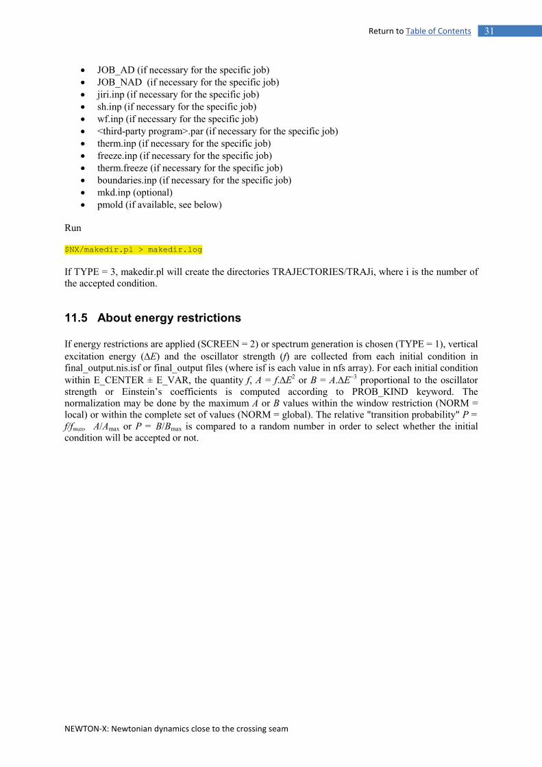
Run $NX/makedir.pl > makedir.log If TYPE = 3, makedir.pl will create the directories TRAJECTORIES/TRAJi, where i is the number of the accepted condition.
11.5 About energy restrictions
If energy restrictions are applied (SCREEN = 2) or spectrum generation is chosen (TYPE = 1), vertical excitation energy (∆E) and the oscillator strength (f) are collected from each initial condition in final_output.nis.isf or final_output files (where isf is each value in nfs array). For each initial condition within E_CENTER ± E_VAR, the quantity f, A = f.∆E2 or B = A.∆E−3 proportional to the oscillator strength or Einstein’s coefficients is computed according to PROB_KIND keyword. The normalization may be done by the maximum A or B values within the window restriction (NORM = local) or within the complete set of values (NORM = global). The relative "transition probability" P = f/fmax, A/Amax or P = B/Bmax is compared to a random number in order to select whether the initial condition will be accepted or not.

NEWTON-X: Newtonian dynamics close to the crossing seam
32 Return to Table of Contents
12 Dynamics inputs
12.1 What is necessary to run
For the input you need the following files: Always: control.dyn - with parameters to control de dynamics. geom - with initial geometry. veloc - with initial velocity. Depending on the settings in control.dyn: jiri.inp - with parameters to control non-adiabatic dynamics. sh.inp - with parameters to control non-adiabatic dynamics. <third-party>.par - with third-party program options. therm.inp - with thermostat options. freeze.inp - with frozen atoms information. therm.freeze - with atoms not affected by thermostat. boundaries.inp - with boundary condition options. NX_analysis - with instructions for customized analysis of the results. stopsign.inp - with instructions to terminate the simulations. You also need the input files for the program that will calculate the energies, gradients and non-adiabatic couplings. JOB_AD - directory containing input files for adiabatic calculation. Energy and gradient for one state. JOB_NAD - directory containing input files for non-adiabatic calculations. Energy, gradient and non-adiabatic coupling. For adiabatic dynamics or non-adiabatic dynamics using time-derivative couplings19, only JOB_AD is necessary. For mixed, non- and adiabatic dynamics (using the THRES keyword), both JOB_AD and JOB_NAD are necessary. For non-adiabatic dynamics using non-adiabatic coupling vectors, only JOB_NAD is necessary.
12.1.1 control.dyn File control.dyn should contain the main parameters for the dynamics: File: control.dyn Namelist: input Parameter Default Description NAT = [3] Number of atoms.
NSTAT = [2] Number of states (dynamics will be performed on the highest one).

NEWTON-X: Newtonian dynamics close to the crossing seam
33 Return to Table of Contents
NSTAT ≥ NSTATDYN.
NSTATDYN = [nstat] Initial state.
NDAMP = [0] 0 : normal dynamics. 1 : velocity is dumped to zero at each time step.
KT = [1] Print output at each KT steps.
DT = [0.5] Time step (fs).
T = [0.0] Initial time (fs).
TMAX = [10.0] Maximum time (fs).
NINTC = [3*Nat-6] Number of internal coordinates to read from the ab intio program. Change default if the system is linear or has redundant coordinates.
MEM = [200] Core memory for the ab initio program (Mwords). (Relevant if PROG = 1)
KILLSTAT = [1] Finish dynamics if after a hopping the system remains more than timekill fs on state KILLSTAT.
TIMEKILL = [0] See KILLSTAT. 0 : deactivate KILLSTAT and TIMEKILL
PROG = [1] Program to compute energies, gradients and non-adiabatic coupling vectors (if available): 0 : Analytical model (see section "Using analytical models") 1 : COLUMBUS 2.0 : TURBOMOLE RI-CC2 / ADC(2) 2.1 : TURBOMOLE TD-DFT 5 : DFTB 6 : GAUSSIAN 7 : TINKER 8 : DFTB+ 10.0 : GAMESS 10.1 : GAMESS ADIABATIC 20 : Hybrid jobs
THRES = [0 for PROG = 2.x and 5] = [100 for PROG = 0, 1 and 6]
Energy difference threshold to initiate non-adiabatic dynamics (eV).
LVPRT = [1] Amount of output to print and output files to keep: 0 : Minimal level 1 : Normal level 2 : Debug level (huge amount of data)
ETOT_JUMP = [0.5] Kill trajectory if total energy deviate more than ETOT_JUMP eV in one time step.
ETOT_DRIFT = [0.5] Kill trajectory if total energy deviate more than ETOT_DRIFT (eV) in comparison to the value in t = 0.
NXRESTART = [0] Restart options: 0: new job. 1: restart job using the content of INFO_RESTART directory. See details in Section 12.4.
[default values] written in inp.f90. Example 1: &input Nat = 6 ! Number of atoms nstat = 3 ! Number of states nstatdyn = 3 ! Initial state

NEWTON-X: Newtonian dynamics close to the crossing seam
34 Return to Table of Contents
dt = 0.5 ! Time step (fs) tmax = 200.0 ! Total time (fs) prog = 2.1 ! Dynamics with TURBOMOLE (TD-DFT). /&end ! Do not forget &input and /&end. Example 2: Ethylene S1-state dynamics, calculating S0, S1 and S2 energies. Time step of 0.1 fs during 200 fs and output printed at each 2 fs. 100,000,000 words of memory. If potential energy difference between two consecutive states drops below 2.0 eV, start non-adiabatic dynamics. Finish dynamics if after a hopping to S0, the system remains more than 10 fs on this state. Get energies, gradients and non-adiabatic couplings with COLUMBUS. &input Nat = 6 nstat = 3 nstatdyn = 2 kt = 20 dt = 0.10 tmax = 200.0 mem = 100 thres = 2.0 killstat = 1 timekill = 10.0 /&end Do not forget "&input" and "/&end".
12.1.2 Geometry The geometry input is (free format, au): Name: geom Symbol_1 Z_1 x_1 y_1 z_1 M_1 Symbol_2 Z_2 x_2 y_2 z_2 M_2 : Symbol_nat Z_nat x_nat y_nat z_nat M_nat where Z is the nuclear charge, x,y,z are the Cartesian coordinates, and M, the atomic masses. Example: C 6. -1.27572383 0.00000000 0.00000000 12.00000000 C 6. 1.27572383 0.00000000 0.00000000 12.00000000 H 1. -2.34867651 0.00000000 -1.75798067 1.00782504 H 1. -2.34867651 0.00000000 1.75798067 1.00782504 H 1. 2.34867651 0.00000000 -1.75798067 1.00782504 H 1. 2.34867651 0.00000000 1.75798067 1.00782504
12.1.3 Velocity The velocity input is (free format, au): Name: veloc vx_1 vy_1 vz_1 vx_2 vy_2 vz_2 : vx_nat vy_nat vz_nat Example: 3.226196727134333E-004 -7.803939823701649E-004 3.501212063660452E-004 8.831202616257374E-005 1.103339279899924E-003 -7.468292758584672E-004 -1.994896289256706E-004 4.345679802152278E-004 -6.123248174920957E-004

NEWTON-X: Newtonian dynamics close to the crossing seam
35 Return to Table of Contents
-3.735660908785368E-003 2.225120145326573E-003 1.414904777249870E-003 -2.272632671568894E-003 -2.177375422081543E-003 3.098061686476041E-003 -6.469986389583130E-004 1.402416374342127E-004 2.362055042392439E-003
12.1.4 Freezing atoms Cartesian coordinates of specific atoms can be kept frozen along the dynamics. For that, a list of atoms should be given in a file called freeze.inp. This file should be given together with the other input files. The atoms in the list are identified by its positions in the geom file and the list is blank separated. Example of freeze.inp: 1 3 (Cartesian coordinate of atoms one and three in geom file will not change during the dynamics.) If a file freeze.inp is present in the input, the atoms defined there will also not be affected by the thermostat. The velocity of the atoms to be kept frozen should be set to zero in the veloc file (section 12.1.3). If the velocity of the frozen atoms is not initially set to zero, the program will stop with an error message. Be aware that this algorithm may introduce spurious rotations and translation in the molecule depending on how the initial velocities of the remaining atoms were generated.
12.1.5 Specific input for quantum-chemistry electronic-structure calculations Please, refer to the documentation of each particular program to see details on their inputs. Here, we present a brief summary of the main option that should be selected for some frequent jobs.
12.1.5.1 Which electronic method to use Nonadiabatic dynamics will always demand a compromise between quality and computational costs. In principle, the description of state crossing regions should be described by a multireference method like MRCI. However, often this is not affordable. In many cases (but not always), single references cases like TDDFT or ADC(2) have proven to give an adequate description of the nonadiabatic problem. You may keep the following thumb rules in mind when deciding which method to use in the simulation:
• Crossings between excited states at TDDFT and ADC(2) levels are in general well described if the ground state DFT is still single reference.
• Crossings between excited states will cause convergence problems at CC2 level. • The description of crossings between the first excited state and the ground state is not reliable
at TDDFT, CC2 or ADC(2) levels.
12.1.5.2 Using analytical models Analytical models for potential energies, gradients and non-adiabatic coupling vectors can be used in the molecular dynamics. The analytical model is supposed to be a program in any language that reads molecular geometry from geom and velocities (if needed) from veloc, and writes the potential energies to epot, gradients to grad and grad.all, and non-adiabatic coupling vectors to nad_vectors. The format of each one of these files is described in the section 16.3. If the analytical model requires additional files besides the executable file (for example, parameter inputs) they must be put in JOB_NAD directory. During the dynamics, the content of this directory is copied to the same location as the other NEWTON-X input files. The specific location of the analytical model can be set via analyt.par. The options are given below.

NEWTON-X: Newtonian dynamics close to the crossing seam
36 Return to Table of Contents
Name: analyt.par Parameter Default Description ANMOD [analytical.model] File name of the executable containing the analytical model. There are two built in
options: analytical.model - 2D conical-intersection analytical model by Ferretti et al. 18. tully_models.pl - 1D models by Tully.14
PATH [$NX] Absolute path to ANMOD file.
For ANMOD = tully_models.pl TULLY_MOD [1] Specific model:
1 – Simple avoided crossing 2 – Dual avoided crossing 3 – Extended coupling with reflexion
Example of analyt.par file:
anmod = my_model.x path = /home/model/
The parameters of the built-in models can be set via JOB_NAD directory. The options are given below. ANMOD = analytical.model Name: JOB_NAD/con_int.dat namelist DAT Parameter Default Description α = [3.0]
See Ref. 18.
β = [1.5]
Kx = [0.02]
Ky = [0.10]
∆ = [0.01]
X1 = [4.0]
X2 = [3.0]
X3 = [3.0]
γ = [0.04]
Example of con_int.dat
&DAT alpha=3.0 beta=1.5 kx=0.02 ky=0.10, delta=0.01 x1=4.0 x2=3.0 x3=3.0 gamma=0.04 &END
ANMOD = tully_models.pl Name: JOB_NAD/constants.dat

NEWTON-X: Newtonian dynamics close to the crossing seam
37 Return to Table of Contents
tully_mod = 1 tully_mod = 2 tully_mod = 3 Parameter Default Parameter Default Parameter Default A 0.01 A 0.10 A 6E-4 B 1.6 B 0.28 B 0.1 C 0.005 C 0.015 C 0.9 D 1.0 D 0.06 E0 0.05
Example of constants.dat
A=0.01 B=1.6 C=0.005 D=1.0
The atomic masses must be set directly in the geom file. In the case of Tully’s models, the original work used 2000 me. In geom, it corresponds to 1.09716 amu. Example of geom file for Tully’s models starting at x = -10 a0. H 1.0 -10.000 0.000 0.000 1.09716 The implementation of the Tully’s models in the tully_models.pl program is made in a very modular way, which allows straightforward implementation of other 1D models. Given the diabatic potential energy functions V11 and V22 and the coupling function V12, the relevant adiabatic quantities are: 1) Energies
( ) ( )1/2
2 21,2 11 22 22 11 12
1 1 .2 4
E V V V V V = + ± − +
2) Energy gradients
( ) ( ) ( )
( ) ( )
1/22 211 22 22 11 12
1,2 22 11 12 22 11 12
1,2 1,2
1 1 12 ,2 2 4
0.
dV dV dV dV dVG x V V V V V Vdx dx dx dx dx
G y G z
− = + ± − − + − + = =
3) Nonadiabatic coupling vector
( ) ( ) ( )
( ) ( )
12 12 22 1112 2 2
22 11 22 1112
22 11
12 12
1 1 ,21
0.
dV V dV dVF xV V dx dx dxV VV
V V
F y F z
= − − − − + − = =
To implement a new 1D model, it is enough to modify tully_models.pl to provide the new V11, V22 and V12 and the respective derivative functions.
12.1.5.3 COLUMBUS COLUMBUS 5.9 Adiabatic dynamics: JOB_AD directory Prepare a set of input files for a Columbus job (geometry optimization, one iteration, NROOT option). For MCSCF jobs, prepare input for CI gradient, but set "Maximum excitation level" to 0 in the CIDRT input. It is also possible to use MCSCF gradients, but in this case only single state dynamics are allowed (NSTAT = 1). Non-adiabatic dynamics using non-adiabatic coupling vectors: JOB_NAD directory

NEWTON-X: Newtonian dynamics close to the crossing seam
38 Return to Table of Contents
Prepare input files for a single-point non-adiabatic coupling calculation. Non-Adiabatic dynamics using time-derivative couplings: JOB_AD directory Prepare a set of input files for a Columbus job (geometry optimization, one iteration, NROOT option). For MCSCF jobs, prepare input for CI gradient, but set "Maximum excitation level" to 0 in the CIDRT input. COLUMBUS 7.0 Adiabatic and non-adiabatic (using coupling vectors or time-derivative couplings) dynamics are directly available at the SA-MCSCF and MR-CI levels. All inputs can be performed using the “non-adiabatic coupling” option in COLUMBUS and only the necessary terms are computed for each case. Optionally, adiabatic and time-derivative MR-CI dynamics may still be performed through “geometry optimization”. Please set version=7.0 when using COLUMBUS 7.0. Parameters to control COLUMBUS jobs Name: columbus.par Parameter Default Description VERSION = [5.9] COLUMBUS version
MEM = [200] Core memory for COLUMBUS (Mwords). The same as MEM in control.dyn, but with
priority over it. (1 GB = 134 Mwords). For COLUMBUS 7, MEM is automatically converted into GB.
CIRESTART = [0] 0: do not use previous CI vector 1: use previous CI vector
MOCOEF = [4] 0: use the same mocoef file in all time steps 1: use the mocoef file from the previous time step k: Lagrangean extrapolation of molecular orbitals at order k-1 (k ≤ 11) (see Section 12.1.10)
PRT_MO = [20] Save mocoef file to DEBUG file every PRT_MO timesteps. (Only if mocoef = 1.)
IVMODE = [8] Initial CI-vector generation mode. See COLUMBUS docs (ciudg program) for a list of options. CIRESTART keyword has priority over IVMODE keyword.
CITOL =[“1E-4”] Tolerance for MR-CI calculations
REDUCE_TOL = [1] 0: keep rtolci and rtolbk in ciudgin as CITOL for all states. 1: use CITOL only to NSTATDYN. For all other states use 1E-3. 2: use CITOL only to NSTATDYN. Use 1E-3 for states coupled to NSTATDYN according to transmomin Columbus file. For all other states use 1E-1. Note that energies computed with 1E-1 are not reliable estimates. Although they are written to the output files, they do not have significance.
MC_CONV = [0] If mcscf calculation do not converge: 0: warn and continue 1: kill trajectory
CI_CONV = [0] If CI calculation do not converge: 0: warn and continue 1: kill trajectory
QUAD_CONV = [60] Set value of NCOUPL in mcscfin
MULL_POP = [0] 1: print out the Mulliken populations from the COLUMBUS calculation to nx.log

NEWTON-X: Newtonian dynamics close to the crossing seam
39 Return to Table of Contents
12.1.5.4 TURBOMOLE Adiabatic dynamics: JOB_AD directory Prepare a set of input files for a TURBOMOLE job at TD-DFT or CC2 level without symmetry and copy them to JOB_AD directory. The initial geometry (TURBOMOLE coord file), the number of states (TURBOMOLE control file), and the state for which the gradient should be computed (TURBOMOLE control file) are automatically set by NEWTON-X during the program execution, overwriting the options in JOB_AD. For TD-DFT dynamics, TURBOMOLE control file is automatically changed to have: $soes all NSTAT-1 $exopt NSTATDYN-1 For RI-CC2 or ADC(2) dynamics, TURBOMOLE control file is automatically changed to have: $excitations irrep=a nexc=NSTAT-1 exgrad states=(a NSTATDYN-1) If TURBOMOLE auxbasis file is provided in JOB_AD, NEWTON-X assumes that the resolution-of-identity (RI) should be used. For CC2 or ADC(2) dynamics, auxbasis must be always provided and the ricc2 program is invoked every time step. For DFT dynamics, the presence of auxbasis file is optional. If it is provided, ridft program is invoked, otherwise dscf program is invoked. The NEWTON-X input for CC2 and ADC(2) dynamics are exactly the same. The only difference is in the TURBOMOLE control file within JOB_AD directory, which should be adequate to the desired method. During the execution, NEWTON-X search for ADC(2) keyword in the TURBOMOLE control file. If it is not found, the CC2 ground state energy is used. If it is found, MP2 ground state energy is used. If you want to perform only adiabatic dynamics, set THRES = 0 (default in control.dyn file) to avoid that NEWTON-X starts the non-adiabatic dynamics calculations. The TURBOMOLE mos file is not updated during the dynamics. Non-Adiabatic dynamics: JOB_AD directory Prepare the TURBOMOLE input files as explained in the previous item. The nonadiabatic dynamics options are described in section 12.1.7. Set THRES = 100 in control.dyn file. Parallel Turbomole (SMP) If you have the SMP parallelized version of Turbomole executables available (dscf_smp, grad_smp, egrad_smp and ricc2_smp) you can use them by specifying parallel = <ncores> in the file turbomole.par with <ncores> being the number of cores to use. The environment variable $OMP_NUM_THREADS is set automatically according to this number and needs not to be set by the user. Parameters to control TURBOMOLE jobs Name: turbomole.par Parameter Default Description

NEWTON-X: Newtonian dynamics close to the crossing seam
40 Return to Table of Contents
PARALLEL = [1] Number of cores to use for parallel Turbomole (smp, no mpi!)
Inputs for old versions of NEWTON-X For NEWTON-X versions prior the 1.0.8, additional input files should be provided for TD-DFT simulations if NSTATDYN = 1 and NSTAT > NSTATDYN. In this case, the following files are required in JOB_AD directory: control.opt - TURBOMOLE control file for ground state gradient (GRAD) calculation. control.sp - TURBOMOLE control file for excited state single point (ESCF) calculation. For excited state gradient calculations (NSTATDYN > 1), no additional files are needed.
12.1.5.5 DFTB Adiabatic dynamics in the ground and excited states can be performed using the time-dependent density functional theory tight binding (TD-DFTB) method. Information about the program can be obtained at www.dftb.org. Input for ground state dynamics: JOB_AD directory Prepare DFTB input for conjugated-gradient ground-state calculation (code 4 in the DFTB program). The DFTB input and geometry information must be called dftb.in and in.gen, respectively. Input for excited-state dynamics: JOB_AD directory Prepare TD-DFTB input for conjugated-gradient excited-state calculation (code 4 in the DFTB program). The DFTB input and geometry information must be called dftb.in and in.gen, respectively. Parameters to control the DFTB jobs Name: dftb.par Parameter Default Description DFTB_EXEC [dftb] Name of the DFTB executable file. $DFTB variable must be defined in the system.
NEWTON-X will run $DFTB/<dftb_exec>.
OTHER_STATE [1] It is possible to perform dynamics on one surface, and at the same time to keep track of the properties of other states (energies and oscillator strengths). In this case, however, DFTB must run twice per time step, which makes the calculation more expensive. 0 - Do not monitor other states 1 - Monitor other states
MULT [S] Multiplicity of the states. Only states with the same multiplicity are allowed. S - singlet T - triplet
12.1.5.6 GAUSSIAN CASSCF level Surface-hopping non-adiabatic dynamics between the ground and the first excited state can be performed at CASSCF level with GAUSSIAN 03. Content of JOB_NAD directory

NEWTON-X: Newtonian dynamics close to the crossing seam
41 Return to Table of Contents
Prepare input files for a single point conical intersection calculation at CASSCF level. The input file must be called gaussian.com and the geometry must be given in Cartesian coordinates. The check point file named gaussian.chk containing the initial molecular orbitals must be provided as well. A suitable example of gaussian.com content is: %chk=gaussian %mem=20000000 #P OPT=(Conical,MaxCycle=1) CAS(4,3) IOp(5/7=200) Guess=read 3-21G Nosymm methaniminium 1 1 N 0.000000 0.000000 0.637342 C 0.000000 0.000000 -0.703614 H -0.648747 0.572349 1.177883 H 0.648745 -0.572350 1.177883 H 0.618844 0.701080 -1.278050 H -0.618844 -0.701080 -1.278049 Note that OPT=(Conical,MaxCycle=1), Nosymm and Guess=read keywords and options should be given exactly as in this example. IOp(5/7=MaxIt) controls the maximum number of iterations in the CASSCF calculation. Parameters to control GAUSSIAN jobs Name: g03.par Parameter Default Description MOCOEF = [1] 0: use the initial molecular orbitals in all time steps
1: use the check point file from the previous time step as the source of molecular orbitals
PRT_MO = [20] Save gaussian.chk file to DEBUG file every PRT_MO timesteps. (Only if mocoef = 1.)
NEWTON-X executes GAUSSIAN 03 by invoking the command: . $g03root/g03/bsd/g03.profile;$g03root/g03/g03 gaussian.com If this path is not adequate for your system, you can change it in $NX/run-g03.pl program. TDDFT level Surface-hopping non-adiabatic dynamics with an arbitrary number of states can be performed at TDDFT level with GAUSSIAN 09. Content of the JOB_AD directory Prepare input files for a single point calculation at TDDFT level. The input file must be called gaussian.com and an optional check point file named gaussian.chk. For nonadiabatic dynamics, NEWTON-X calls rwfdump program of Gaussian. $g09root/g09/bsd/g09.login should be sourced either in the user profile or in the submission script before running the job. To run a calculation in parallel, the number of processors has to be specified with the keyword %nproc in the GAUSSIAN input. It has also to be specified in the submission script. In file gaussian.com, the DFT functional, basis set and TD keyword with the proper options should be specified. The user should not use the keywords Guess=Read and TD(Read) in the input file.

NEWTON-X: Newtonian dynamics close to the crossing seam
42 Return to Table of Contents
These options must be defined in g09.par file (see below). NEWTON-X adds NoSymm keyword automatically to avoid any problems due to differences between input and standard orientations. The basis set may be directly given in the route or defined through GEN keyword. For nonadiabatic dynamics, the basis set must be also provided in an additional file called basis. Different ways of defining the basis sets are illustrated in the next examples. • Example 1: The simplest case. The same basis set is used for all atoms and it is defined in the GAUSSIAN library. Example of content of gaussian.com file: %chk=gaussian %rwf=gaussian %mem=200mw #TD(Nstates=3,Root=2) 3-21G BHandHLYP nosymm test bs1 0 1 Si -0.010544 0.010835 0.808752 C 0.015819 -0.050721 -0.931069 H 0.009875 1.149573 1.543340 H 0.172225 -1.176299 1.509994 H 0.071356 1.042598 -1.452426 H -0.149187 -0.712162 -1.664254
Example of basis file: 3-21G In this example, there is a redundancy in the basis set definition, which appears in gaussian.com and in basis. You should carefully check whether both files contain the same definitions. • Example 2: Basis set is not defined in the GAUSSIAN library. Then you have to use the GEN keyword in gaussian.com and provide the basis set. In addition you have to copy the basis set to the basis file. Example of GAUSSIAN input: %chk=gaussian %rwf=gaussian %mem=200mw #TD(Nstates=3,Root=2) GEN BHandHLYP nosymm test bs1 0 1 Si -0.010544 0.010835 0.808752 C 0.015819 -0.050721 -0.931069 H 0.009875 1.149573 1.543340 H 0.172225 -1.176299 1.509994 H 0.071356 1.042598 -1.452426 H -0.149187 -0.712162 -1.664254 H 0 S 2 1.00 5.4471780 0.1562850 0.8245470 0.9046910 S 1 1.00 0.1831920 1.0000000 **** C 0

NEWTON-X: Newtonian dynamics close to the crossing seam
43 Return to Table of Contents
S 3 1.00 172.2560000 0.0617669 25.9109000 0.3587940 5.5333500 0.7007130 SP 2 1.00 3.6649800 -0.3958970 0.2364600 0.7705450 1.2158400 0.8606190 SP 1 1.00 0.1958570 1.0000000 1.0000000 **** Si 0 S 3 1.00 910.6550000 0.0660823 137.3360000 0.3862290 29.7601000 0.6723800 SP 3 1.00 36.6716000 -0.1045110 0.1133550 8.3172900 0.1074100 0.4575780 2.2164500 0.9514460 0.6074270 SP 2 1.00 1.0791300 -0.3761080 0.0671030 0.3024220 1.2516500 0.9568830 SP 1 1.00 0.0933392 1.0000000 1.0000000 **** Content of basis file: H 0 S 2 1.00 5.4471780 0.1562850 0.8245470 0.9046910 S 1 1.00 0.1831920 1.0000000 **** C 0 S 3 1.00 172.2560000 0.0617669 25.9109000 0.3587940 5.5333500 0.7007130 SP 2 1.00 3.6649800 -0.3958970 0.2364600 0.7705450 1.2158400 0.8606190 SP 1 1.00 0.1958570 1.0000000 1.0000000 **** Si 0 S 3 1.00 910.6550000 0.0660823 137.3360000 0.3862290 29.7601000 0.6723800 SP 3 1.00 36.6716000 -0.1045110 0.1133550 8.3172900 0.1074100 0.4575780 2.2164500 0.9514460 0.6074270 SP 2 1.00 1.0791300 -0.3761080 0.0671030 0.3024220 1.2516500 0.9568830 SP 1 1.00 0.0933392 1.0000000 1.0000000 In this case, the basis set defined in basis will be used in the dynamics even if gaussian.com has a different definition.
• Example 3: Different basis sets for different atoms. GEN keyword is also needed in this case. Example of GAUSSIAN input:

NEWTON-X: Newtonian dynamics close to the crossing seam
44 Return to Table of Contents
%chk=gaussian %rwf=gaussian %mem=200mw #TD(Nstates=3,Root=2) GEN BHandHLYP nosymm test bs1 0 1 Si -0.010544 0.010835 0.808752 C 0.015819 -0.050721 -0.931069 H 0.009875 1.149573 1.543340 H 0.172225 -1.176299 1.509994 H 0.071356 1.042598 -1.452426 H -0.149187 -0.712162 -1.664254 Content of basis file: 1 0 6-31G(d) **** 2 0 6-31G(d) **** 3 0 3-21G **** 4 0 3-21G **** 5 0 6-31G **** 6 0 6-31G In this case, the basis set defined in basis will be used in the dynamics even if gaussian.com has a different definition. Parameters to control GAUSSIAN jobs Name: g09.par Parameter Default Description MOCOEF = [0] 0: compute the initial guess at every time step.
1: use the check point file from the previous time step as the source of molecular orbitals. 2: use the initial molecular orbitals in all time steps.
TD_ST = [0] 0: compute the excited states without previous reference. 1: read the states from the checkpoint file, the checkpoint file is controlled by MOCOEF (1 or 2). We don’t recommend using this option in non-adiabatic dynamics calculations.
PRT_MO = [20] Save gaussian.chk file to DEBUG file every PRT_MO timesteps.
LD_THR = [14] N: Controls the linear dependency threshold (10-N) in G09 calculations. NEWTON-X executes GAUSSIAN 09 by invoking the command: . $g09root/g09/bsd/g09.profile;$g09root/g09/g09 gaussian.com If this path is not adequate for your system, you can change it in $NX/run-g09.pl program.
12.1.5.7 TINKER

NEWTON-X: Newtonian dynamics close to the crossing seam
45 Return to Table of Contents
Adiabatic ground-state dynamics with forcefield-gradients and –energies can be performed with TINKER. Content of the JOB_AD-directory An TINKER-XYZ file called tinkin.xyz and the corresponding keyword-file tinkin.key have to be present. The file tinkin.key has to state at least the name of the parameter file ('parameters <filename>') and 'digits 12'. The command executed by NEWTON-X is testgrad tinkin.xyz –k tinkin.key y n n If the TINKER-executables are not in the $PATH, testgrad.x can also be provided as binary in the JOB_AD directory.
12.1.5.8 DFTB+ Adiabatic dynamics in the ground can be performed using the density functional theory tight binding (DFTB) method. Input for ground state dynamics: JOB_AD directory Prepare DFTB+ input for conjugated-gradient ground-state calculation (code 4 in the DFTB program). The DFTB+ input and geometry information must be called dftb.in and in.gen, respectively. Parameters to control the DFTB+ jobs Name: dftb+.par Parameter Default Description DFTBP_EXEC [dftb+] Name of the DFTB+ executable file. $DFTBPLUS variable must be defined in the system.
NEWTON-X will run $DFTBPLUS/<dftbp_exec>.
12.1.5.9 GAMESS Adiabatic dynamics: JOB_AD directory Prepare a gradient input file for a GAMESS job at some adiabatic level (e.g. CCSD(T) or MP2) without symmetry and copy the file to the JOB_AD directory. The input file should be labeled either gamessinput_original.inp (without the $DATA group) or nx_gamess.inp (with the $DATA group). Either way, starting coordinates for the run always get taken from the NEWTON-X geom file. The initial geometry, the number of states, and the state for which the gradient should be computed are automatically set by NEWTON-X during the program execution. Please ensure the iroot variable (in $det or similar group) in nx_gamess.inp is the same as nstatdyn in control.dyn file. If you want to perform only adiabatic dynamics, set THRES = 0 in control.dyn file to avoid non-adiabatic dynamics calculations. Analytic gradients are available for state-averaged runs and are activated with wtsok=.t. in the $det group ( and no NUMGRD=.t. in $contrl). GAMESS input examples exist in $NX/test-nx. Non-adiabatic dynamics using non-adiabatic coupling vectors: JOB_NAD directory

NEWTON-X: Newtonian dynamics close to the crossing seam
46 Return to Table of Contents
NA couplings are available at the SA-MCSCF level. Specific NA coupling selection schemes are also available through the jiri.inp file with napick=.t. in $cpconv. All NA couplings can be calculated with napick=.f. in $cpconv along with appropriate input to jiri.inp. Prepare input files for a single-point non-adiabatic coupling calculation. Prepare either: 1) gamessinput_original.inp: runtyp=nacme without $DATA and $VEC gamessinput_original.vec: $VEC group 2) nx_gamess.inp: runtyp=nacme with $DATA and $VEC Parameters to control GAMESS jobs Name: gamess.par Parameter Default Description VERNO = [00] Version number of GAMESS executable.
NCPUS = 1 Number of computer processes to be run.
RUN_GAMESS = [rungms] Name of GAMESS execution script.
SCR
= [0] GAMESS scratch directory: 0: Use default GAMESS options as defined in RUN_GAMESS script. 1: Create SCR directory inside TEMP directory of NEWTON-X.
MOCOEF = [1] 0: use the initial molecular orbitals in all time steps 1: use the mocoef file from the previous time step k: Lagrangean extrapolation of molecular orbitals at order k-1 (k ≤ 11) (see Section 12.1.10)
12.1.5.10 Hybrid Gradients (QM/MM) The hybrid gradients module allows adiabatic and non-adiabatic dynamics with combinations of programs (COLUMBUS, TINKER, TURBOMOLE and Analytical Model). The current implementation is described in Ref.36.
General explanations of hybrid calculations
Energies and gradients for subsets of atoms are treated with different programs and the partial gradients are then joint into a resulting total (hence 'hybrid') energy and gradient. For that purpose the set of atoms of the whole system is split in disjoint regions. These regions need not follow physical reasoning (they often will, but the can also pick e.g. single atoms out of molecules), but are logical entities for the definition of the single partial calculations. The whole calculation is split into jobs. Each of these jobs can treat one or more regions of atoms and the partial result are multiplied by a user-defined factor before being added to the total. One region can be treated by multiple jobs and to care about 'double counting' of atoms is left to the user completely. For COLUMBUS and TURBOMOLE there is the possibility to include regions only as point charges and not as atoms with basis-set. A hybrid setup (which is done in the JOB_AD or JOB_NAD directory) consists of some general information about the hybrid setup ('control' parameters), the

NEWTON-X: Newtonian dynamics close to the crossing seam
47 Return to Table of Contents
definition of the atoms, some of their properties and membership to the regions and the definition of the partial jobs, which regions they are concerned with and how they shall be put together to the overall result. The main input file is named hybrid_gradients.inp. The nonadiabatic couplings, oscillator strengths and other nonadditive properties are given by only one job. It is possible to restrict the hybrid NAD-vectors to some regions. The NAD-vector components on all atoms not belonging to these regions are replaced by Zeros in this case. Also for back hoppings only the kinetic energy of these nad-regions is regarded as available energy. For the treatment of bonded interaction between two regions link atoms can be inserted in bond connecting them. The gradient- and nonadiabatic coupling vector elements of these link atoms will be distributed to the two atoms between which it has been inserted. To avoid over-polarization effects, the point charges near the link atom can be set to zero and, so as to retain the overall charge, re-distributed to a set of other atoms. The job, where the link atom is inserted is (suggestively) called ‘QM_JOB’ regardless of the method really used in this job. Similarly is the naming of ‘QM_ATOM’ and ‘MM_ATOM’.
Format of the hybrid_gradients.inp file
Each section begins with $<name> and ends with $end, where <name> can be 'control', 'job' or 'atoms'. Parameters for sections '$control' and '$job' are set in key=value pairs. All key=value pairs have to be separated with blanks. Name: hybrid_gradient.inp Section Keyword Description $control NATOMS number of atoms (optional)
PROPERTIES ID of the job, that gives the properties (oscillator strength,
nonadiabatic couplings, optional)
NADREGIONS array of regions to which the hybrid nad-vector shall be restricted
$job ID unique numeric (integer) identification for the job
PROGRAM name of the program to be used for this job (columbus, tinker, turbomole)
REGIONS array of regions, that shall be treated by this job (comma seperated)
FACTOR pre-factor with that the result of this job enters the total result (energy, gradients)
POINTCHARGES array of regions, that shall be treated as point-charges (for columbus and turbomole, comma seperated, optional)
$atoms (For each atom give in one single line and in this order:) <name> Label for an atom (compulsory). Can be anything without blanks,
comma and similar. The type of atom is recognized from the nuclear charge.
<nuclear charge> Nuclear charge.
<x,y,z coords> Cartesian coordinate (Bohr).
<pointcharge> Effective point charge for this atom. If this atom is not treated as point charge this can be left to 0.0000.
<mass> Atomic mass for this atom (amu).
<region> The region in which this atom is.

NEWTON-X: Newtonian dynamics close to the crossing seam
48 Return to Table of Contents
link QM_JOB ID of the job where the link atom shall be inserted.
QM_ATOM number (=position in input) of the atom connected to the link atom at the QM-side.
MM_ATOM number (=position in input) of the atom connected to the link atom at the MM side.
RATIO ratio of distances QMat→LINKat/QMat→MMat.
ZERO comma seperated list of atoms for which the point charge shall be set to 0.000 in the QM_JOB.
SCATTER comma seperated list of atoms to which the accumulated charge of the ZERO-atoms shall be distributed.
The section $atoms is an extension of the NEWTON-X geom. with the two additional columns, <pointcharge> and <region>. Each atom has to be in exactly one region. All values in section $atoms have to be separated with blanks. Every section has to be ended with $end. No section (except '$jobs') is allowed to appear twice. There are no further formatting rules to the file. Example of hybrid_gradient.inp file: $job ID = 1 regions = 1,2 program = columbus pointcharges = 2 factor = 1 $end $job ID = 2 regions = 1,2 program = tinker factor = 1 $end $job ID = 3 regions = 1 program = tinker factor = -1 $end $control properties = 1 nadregions = 1 natoms = 9 $end $atoms C 6.0 -0.58698100 -0.10086826 0.12744020 12.00000000 0.0000 1 O 8.0 1.68492145 0.00195156 0.55748655 15.99491464 0.0000 1 N 7.0 -1.73272850 -2.27661770 -0.35180374 14.00307401 0.0000 1 H 1.0 -1.76941972 1.58570542 0.11857328 1.00782504 0.0000 1 H 1.0 -3.64014444 -2.31932440 -0.70744017 1.00782504 0.0000 1 H 1.0 -0.69532029 -3.86742067 -0.35771869 1.00782504 0.0000 1 OW 8.0 -6.90020375 -2.40598424 -1.31691242 15.99491464 -0.8340 2 HW 1.0 -7.75621060 -2.20340156 -2.90625351 1.00782504 0.4170 2 HW 1.0 -8.26652850 -2.54571452 -0.12804111 1.00782504 0.4170 2 $end
This example is explained in details in the NEWTON-X tutorial. Example including link atoms (some lines not displayed): # 2-butene with cyclohexane rings attached to the sides # Z2-scheme is used for point charges,i.e. first and second # neighbour to the link atom have zero charges and the # their charge is distributed to their next-neighbours on the MM side $job ID=1 regions=1,2,3 program=turbomole turbo_method=td-dft pointcharges=2,3 factor=1 $end $job ID = 2 regions = 1,2,3 program = tinker factor = 1 $end $job ID = 3 regions = 1 program = tinker factor = -1 $end $link qm_job=1 qm_atom=1 mm_atom=11 ratio=0.713 zero=11,12,13,14 scatter=15,16,17 $end $link qm_job=1 qm_atom=4 mm_atom=34 ratio=0.713 zero=34,35,36,37 scatter=38,39,40 $end $control properties = 1 nadregions=1 natoms = 56 $end $atoms C 6.0 1.44087838 0.85091533 -3.47469613 12.00000000 0.0000 1 #atom 1 # linked to atom 11 C 6.0 1.23567680 -0.48733580 -6.00452731 12.00000000 0.0000 1 C 6.0 2.80448775 -2.25355699 -6.92713507 12.00000000 0.0000 1 C 6.0 5.12903987 -3.34336584 -5.64481794 12.00000000 0.0000 1 #atom 4 # linked to atom 34 H 1.0 1.17513186 2.91664300 -3.78035178 1.00782504 0.0000 1 H 1.0 3.36724819 0.62483228 -2.66873550 1.00782504 0.0000 1 H 1.0 -0.40125500 0.07262218 -7.17351567 1.00782504 0.0000 1

NEWTON-X: Newtonian dynamics close to the crossing seam
49 Return to Table of Contents
H 1.0 2.39776578 -3.02448967 -8.82452971 1.00782504 0.0000 1 H 1.0 4.98819669 -5.44423296 -5.69313068 1.00782504 0.0000 1 H 1.0 5.18046121 -2.82088113 -3.61093594 1.00782504 0.0000 1 CT 6.0 -0.52739233 -0.13060275 -1.57905516 12.00000000 -0.1200 2 #atom 11 HC 1.0 -0.25927609 -2.20323737 -1.33315643 1.00782504 0.0600 2 HC 1.0 -2.45999068 0.14865342 -2.36823880 1.00782504 0.0600 2 CT 6.0 -0.33457412 1.20138205 0.99721226 12.00000000 -0.1200 2 HC 1.0 1.56440222 0.83732631 1.83045298 1.00782504 0.0600 2 HC 1.0 -0.45614398 3.28079700 0.68304340 1.00782504 0.0600 2 : : : : : : : : : : : :# lines omitted CT 6.0 -2.23690095 2.08870485 5.28849685 12.00000000 -0.1200 2 HC 1.0 -0.32070164 1.91506358 6.14394752 1.00782504 0.0600 2 HC 1.0 -2.48154867 4.11306830 4.76133507 1.00782504 0.0600 2 CT 6.0 7.60087913 -2.51304285 -6.92702736 12.00000000 -0.1200 3 #atom34 HC 1.0 9.21362621 -3.51540650 -6.01449183 1.00782504 0.0600 3 HC 1.0 7.56925645 -3.13134234 -8.93790950 1.00782504 0.0600 3 CT 6.0 8.05428868 0.35505686 -6.77227957 12.00000000 -0.1200 3 HC 1.0 7.92399962 0.94155983 -4.75349648 1.00782504 0.0600 3 HC 1.0 6.51305828 1.36826754 -7.78612331 1.00782504 0.0600 3 CT 6.0 10.63311478 1.21580066 -7.83079266 12.00000000 -0.1200 3 HC 1.0 12.15373961 0.13167423 -6.84744154 1.00782504 0.0600 3 : : : : : : : : : : : :# lines omitted $end
Generating and updating the remaining input files
After having written hybrid_gradient.inp file, the complete set of input files can be created by run $NX/hybrid_read_onefile.pl Subdirectories for the different jobs will be created as well. Appropriate geom files for each job are provided in these subdirectories. Set up the third-party single jobs inputs in the subdirectories in the same way as for normal NEWTON-X dynamics. If you chose to include some atoms as point-charges to a COLUMBUS- or TURBOMOLE-job you have to set the jobs up appropriately. Refer to the documentations of the programs for information on how to do that (hybrid_read_onefile.pl will provide some useful files containing most of things, that have to be done extra to a normal setup). In the subdirectories for partial hybrid jobs to be computed with COLUMBUS including point-charges two files 'potential.xyz' and 'elpotin' are provided. Do not delete these files! In the subdirectories for partial hybrid jobs to be computed with TURBOMOLE including point-charges two files ‘pointcharges’ and ‘control-additions’ are provided. Do not delete the pointcharges-file. The contents of the file ‘control-additions’ have to be inserted in the control-file at an appropriate position after setting up the TURBOMOLE calculation. If any change is done to hybrid_gradient.inp, hybrid_read_onefile.pl should be run again to update the remaining files.
12.1.6 Thermostat control Thermal-equilibration may be obtained during the dynamics by using a thermostat 35. In the current NEWTON-X version, the Andersen thermostat is available 34. The Andersen-Lowe thermostat 48 is being implemented and it will available soon. The parameters of the thermostat may be adjusted by using nxinp tool, in the input section “Set General Options”. The options are given below. Name: therm.inp namelist therm Parameter Default Description KTHERM = [1] Thermostat type:
0 - No thermostat. 1 - Andersen 34. 2 - Andersen-Lowe 48 (in development).

NEWTON-X: Newtonian dynamics close to the crossing seam
50 Return to Table of Contents
TEMP = [300] Temperature (K).
KTS = [1] Turn the thermostat on at time step KTS. (KTS ≥ 1, integer)
LTS = [-1] Turn the thermostat off at time step LTS. (LTS > KTS, integer) -1 - Do not turn it off.
NSTHERM = [1] If the system is in the excited state: 0 - turn the thermostat off. 1 - apply the thermostat.
GAMMA = [0.2] Collision frequency (fs-1).
RADIUS = [10.0] Collision radius (bohr). (Only in Andersen-Lowe thermostat.)
ISEED = [1] Random number seed for the thermostat. 0 - default seed value. 1 - generate random seed. > 1 - use this value (integer) as the seed.
LVP = [1] Print level. (In any case, relevant information is written to NEWTON-X log.) 1 - Do not print thermostat log file. 2 - Print minimum thermostat log file. 3 - Print debug-level thermostat log file.
Example of therm.inp file: &therm ktherm = 1 kts = 1 lts = -1 nstherm = 1 temp = 300 gamma = 0.6 iseed = 0 lvp = 3 &end You can choose a subset of atoms that will not be affected by the thermostat. For that, a list of atoms should be given in a file called therm.freeze. This file should be given together with the other input files. The atoms in the list are identified by its positions in the geom file and the list is blank separated. Example of therm.freeze: 1 3 (Atoms one and three in geom file will not be affected by the thermostat.) If a file freeze.inp is present in the input, the atoms defined there will also not be affected by the thermostat (see section 12.1.4).
12.1.7 Non-adiabatic dynamics control The non-adiabatic dynamics is controlled by two input files, sh.inp and jiri.inp. SH is a stand-alone module for surface-hopping. It reads nuclear velocities and non-adiabatic couplings and gives as output the electronic wavefunction expansion coefficients on the adiabatic set of states. Switch from one adiabatic PES to another is ruled by the Tully's fewest switches algorithm 14. The parameters for non-adiabatic dynamics can be set via nxinp tool, at the input option “Set non-adiabatic dynamics”. The options are given below. Name: sh.inp namelist shinp

NEWTON-X: Newtonian dynamics close to the crossing seam
51 Return to Table of Contents
Parameter Default Description VDOTH = [0] Dynamics with non-adiabatic coupling vectors or with time-derivative couplings (HST model
19,20). -1 – Local-diabatization method.21 0 - Compute non-adiabatic coupling vectors. 1 - Compute time-derivative couplings (COLUMBUS and TURBOMOLE TD-DFT).19 The default is reset to 1 if PROG = 2.1.
SEED = [1] 0 a default random number seed is used. 1 a randomized seed is used >1 random number seed
INTEGRATOR = [5] selects the integrator of the TDSE: 0 - a "home-made" integrator, see Ref. 18. 1 - standard 4th order Runge-Kutta. 2 - Adams Moulton predictor-corrector, 5th order. 3 - Adams Moulton predictor-corrector, 6th order. 4 - Unitary propagator. 5 - Butcher, 5th order.49 6 – Unitary propagator for Local-Diabatization method. Good choices are usually 3, 4, and 5. For vdoth = -1 (local diabatization) integrator must be 6.
PHASE = [1] Integrate the phase along the trajectory (only for debug purposes): 0 - No. Phase is always zero. 1 - Yes.
NOHOP = [0] Force the hopping at the certain time step. 0 - The trans. prob. are computed and hopping is allowed (normal surface hopping). -1 - Hopping is not allowed at any time. n - Hopping is forced at (and only at) timestep n (n = positive integer).
FORCESURF = [1] Force the hopping to the surface FORCESURF (ground state = 1).
NRELAX = [0] number of cycles after a surface hopping, in which other hopping is forbidden.
MS = [20] number of subtime-steps for integration of the time dependent Schroedinger equations is dt/ms, where dt is the time-step of the classical trajectory defined in control.dyn file. In the ms-1 substeps between t and t+dt, the non-adiabatic coupling vector and the velocity vector is obtained by linear interpolation. The potential energy is interpolated with a cubic polynomial. 0 - Do not interpolate. 1 - Time-step will be divided by one. The results is the same as using ms = 0, but now the interpolation programs are called. For vdoth = -1 (local diabatization), ms must be 0.
GETPHASE = [1] 0 use phase provided by the overlap of CI vectors. 1 use phase provided by the scalar product between h(t) and h(t-dt). Usualy this is the best choice for multistate dynamics.
TULLY = [1] Fewest-switches algorithm: 0 - Tully 14. 1 - Hammes-Schiffer and Tully 20.
DECAY = [0.1] Apply the decoherence correction to the time-dependent coefficients CK of state K 27. The value of DECAY is assumed by the variable α in the equations:
( ) MKtCC KMKK ≠∀∆−= τ/exp'
, 2/1
2
'
'
1
−=
∑≠
M
MKK
MMC
CCC
,
+
−=
kinMKKM EEE
ατ 1
,
where M is the current state and Ekin is the nuclear kinetic energy. α (DECAY) must be given in atomic units (hartree). The recommended value is α = 0.1 hartree. -1 means normal

NEWTON-X: Newtonian dynamics close to the crossing seam
52 Return to Table of Contents
calculation (without correction). After integrating the TDSE to obtain the coefficients C and using the fewest-switches to determine the current state M, the equations above are used to obtain the coefficients C’. The C’ are then used to continue the time evolution of the electronic wave function.
PROBMIN = [0] Do not hop if probability is smaller than PROBMIN.
MOM = [1] After a frustrated hopping: -1 - Invert momentum direction. 1 - Keep momentum direction.
ADJMOM = [0] After a hopping adjust momentum: -1 - along the momentum direction. 0 - along the non-adiabatic coupling vector h. 90 - along the gradient difference vector g. For any value larger or equal to 0, ADJMOM is assumed to be an angle α in degrees, which defines the unitary vector
( ) ( )hh
gg
ααε cossinˆ +=.
The momentum is adjusted in the direction of ε̂ . Note: Until NEWTON-X version 0.10a, the definition of ADJMOM and the default value were different. Check old input files before running. The default is reset to -1 if VDOTH = 1.
POPDEV = [0.05] Kill trajectory if total adiabatic population deviate more than POPDEV from the unity.
Example of sh.inp file: &shinp seed=0, integrator=4, nrelax=0, ms=10, getphase=1, &end The following keywords in jiri.inp file allow additional control over the non-adiabatic coupling calculations by restricting which states should be included in the calculations. In combination with THRES defined in control.dyn, it is possible to substantially reduce the computational costs by excluding couplings that should not contribute to the hopping probabilities19. The default (THRES = 0, KROSS = 1, CASCADE = 0, CURRENT = 1, NEVER_STATE = 0, INCLUDE_STATE = 0) implies that all possible coupling vectors between the current and the other states will be computed. When time derivative couplings are used (VDOTH = 1), the default of NEVER_STATE = 1, meaning that non-adiabatic coupling with the ground state are not computed. Internally, the restrictions implied by these keywords are independently applied to the complete list of NC = Nstat(Nstat-1)/2 possible coupling vectors and the result is a restricted list of couplings. This information is written every timestep to the file transmomin. Thus, the list of coupling vectors that should be computed is dynamically updated along the simulation. If a transmomin file is given with the input in JOB_NAD it will be replaced by the new one already in step 0. Name: jiri.inp Namelist: jirinp Parameter Default Description KROSS = [1] 0 - do not calculate non-adiabatic couplings between non-
consecutive states. For example, between S0 and S2. 1 - calculate non-adiabatic couplings between non-consecutive states.

NEWTON-X: Newtonian dynamics close to the crossing seam
53 Return to Table of Contents
CASCADE = [0] Compute non-adiabatic couplings only for states below the current state and state: 0 - above and below (e.g., in S2 get S2-S1 and S2-S3) 1 - only below (e.g., in S2 get S2-S1 but not S2-S3)
CURRENT = [1] Compute non-adiabatic couplings only for pairs of states including the current state.
NEVER_STATE = [0] Array of states for which the non-adiabatic coupling vectors should never be computed. E.g., if never_state=1,2: don't compute couplings with S0 or S1 (1 – ground state). The array must be coma separated. The maximum number of states in the array is 10. The default (0) means do not exclude any state. The default is 1 when VDOTH = 1.
INCLUDE_PAIR = [0] Define the pairs of states for which the non-adiabatic coupling vector for the following pairs should be always computed, when the current state is one of the states in the pair. E.g., include_pair=1,2,1,3: when the molecule is in S0, always compute couplings S0-S1 and S0-S2 (1 – ground state). The array must be coma separated. The maximum number of pairs is 5.
E_CI = [0.2] Check the energy difference between every pair of states and report it when this difference drops below the e_ci threshold (in eV). The information is written to RESULTS/report.CI and it is useful to locate conical intersections.
If VDOTH = 1 in sh.inp: CI_CONS = [1] 0 - Compute all determinant overlap terms.
1 - Neglect determinant overlap terms when the hank is too high or when the determinants are orthogonal.
CIO_OPTIONS COLUMBUS: =[“-t 1e-5 -e 2 -i”] TDDFT, TURBOMOLE: =[“-s transmomin -a -t 5e-5 -e -1”]
Options to the cioverlap program (given in quotation marks). See detailed description in section 16.6.
CISC_OPTIONS = [„-O -C“] Options to the cis_casida program (given in quotation marks). See detailed description in section 16.6
NCORE = [0] Number of core orbitals that should be ignored in the CIS Casida procedure (using the -i option of the cis_casida executable).
NDISC = [0] Number of virtual orbitals that should be ignored in the CIS Casida procedure (using the -I option of the cis_casida executable).
Example of jiri.inp file: &jirinp kross = 0 cascade = 1 /&end Do not forget "&jirinp" and "/&end". There are eight possible combinations of the keywords KROSS, CASCADE and CURRENT. Each one corresponds to a different model. The models are called: two-state (TS), three-state (3S), horizontal coupling (HC), lower diagonal (LD), partial coupling (PC), neighbour coupling (NC), lower triangular, and complete coupling (CC)19. In the Table below, the keyword combination for each of these models is given, as well as the number Nc of coupling vectors computed in each time step. An example of which coupling vectors are actually computed in the case of dynamics with Nstat = 5 states

NEWTON-X: Newtonian dynamics close to the crossing seam
54 Return to Table of Contents
with the molecule instantaneously in Nstatdyn = 3 state is also shown in the Table. The bold line shows the default option.
kross cascade current Model Nc Example: NSTAT=5,NSTATDYN=3 21 31 32 41 42 43 51 52 53 54 0 1 1 TS 1 x 0 0 1 3S 2 x x 1 1 1 HC Nstatdyn-1 x x 0 1 0 LD Nstatdyn-1 x x 1 0 1 PC Nstat-1 x x x x 0 0 0 NC Nstat-1 x x x x 1 1 0 LT Nstatdyn(Nstatdyn-1)/2 x x x 1 0 0 CC Nstat(Nstat-1)/2 x x x x x x x x x x
In addition to these eight models, other combination can be built by using the keywords NEVER_STATE, INCLUDE_PAIR, and THRES (in control.dyn). For example, the following jiri.inp: &jirinp kross = 0 cascade = 1 current = 1 include_pair = 1,2 /&end will result in a modified TS model for which the coupling vector from state 1 (ground) to state 2 is computer whenever the molecule is in state 1.
12.1.8 Time-derivative couplings Dynamics using time-derivative couplings to compute the non-adiabatic surface hopping probabilities can be performed with COLUMBUS (MCSCF, MRCI) and TURBOMOLE (TD-DFT). The method was proposed by Hammes-Schiffer and Tully 20 and the current implementation is described in Ref.19. For TD-DFT this method should be used exclusively for surface hopping between excited states, because the linear-response TD-DFT cannot adequately describe the mutireference character of the electronic wavefunction near conical intersections between the ground and the first excited state.
12.1.9 Wave function coefficients The real and imaginary parts of the coefficients of the time dependent Schroedinger equation are automatically updated to the file wfrun during the dynamics. The default is to start the dynamics with 1.0 at the initial state and 0.0 for all other states. It is possible to change this default by just including wf.inp as an additional input file, with the format: Re(C_1) Im(C_1) Re(C_2) Im(C_2) ... Re(C_NSTATDYN) Im(C_NSTATDYN) ... Re(C_NSTAT) Im(C_NSTAT) For example, the default for a two-state dynamics (S0 and S1), starting in S1 is: 0.0 0.0 1.0 0.0 One possibility to start with 20% at S2 and 80% in S1 is: 0.894427191 0.0 0.447213596 0.0

NEWTON-X: Newtonian dynamics close to the crossing seam
55 Return to Table of Contents
12.1.10 Propagation of molecular orbitals The keyword MOCOEF appearing in some of the <third-party>.par files controls how the molecular orbital coefficients are transferred from on step to the following. The original (time step n = 0) coefficients may be used, or the coefficients from step n may be given as guess for step n+1 (COLUMBUS, GAUSSIAN, AND GAMESS). A set of k molecular orbital coefficients computed between steps n-k and n can also be extrapolated to create the guess for step n+1 (COLUMBUS AND GAMESS). This is done by means of Lagrangean Extrapolation of Molecular Orbitals (LEMO) algorithm described in Ref. 33. Briefly the molecular orbital coefficient guess (cguess) for step n+1 is given in terms of the previously converged coefficients (cconv) by
∑−
=
−−
+ =1
0,,,1
1,,
k
l
lnjiconvlk
njiguess cLc (1≤ i ≤ nbas, 1≤ j ≤ nbas),
where L is the set of Lagrangean coefficients for polynomial interpolation and nbas is the number of basis functions. The treatment of orbital rotations in the version of LEMO algorithm implemented in NEWTON-X differs from the one proposed in Ref. 33. In NEWTON-X, the overlap factor
( )∑
∑
=
=
−
− =bas
bas
n
j
njiconv
n
j
knjiconv
njiconv
knni
c
ccS
1
2,,
1,,,,
, (1≤ i ≤ nmo)
is computed for a sub-set of nmo orbitals, usually the occupied ones. If knniS −, < Smin, then the orbital i is
not extrapolated and it is given by n
jiconvn
jiguess cc ,,1
,, =+ . In the current version, nbas and nmo are automatically set by NEWTON-X reading the COLUMBUS input files. Smin is set to 0.7. For a given extrapolation order k-1, k sets of molecular orbital coefficients are necessary. In the beginning of the dynamics, while the step number is still smaller than k, the LEMO algorithm is executed at lower extrapolation order, using the molecular orbital sets available.
12.1.11 Boundaries The system can be included in rigid boundaries (at the moment only spherical). If the file ‘boundaries.inp’ is present in the treatment of boundaries is activated. In the spherical boundary, if any molecule attempts to move outwards, it undergoes an elastic collision and their radial velocity is inverted. Name: boundaries.inp Parameter Description INSPHERE Include system in a rigid sphere.
At the second line give the radius and Cartesian coordinates for the center of the sphere in Bohr. rr.r xx.x yy.y zz.z
12.1.12 Stop conditions It is possible to define quite arbitrary set of conditions that when satisfied will cause the end of the simulations. This is done through a series of conditions connected by logic operators written to stopsign.inp file.

NEWTON-X: Newtonian dynamics close to the crossing seam
56 Return to Table of Contents
Each condition X (integer) with operator Y (and, or) is defined by four keywords. Name: stopsign.inp Parameter Description %comm_Y[X] Single line Perl command to collect information to be checked. %text_Y[X] Description of the command. %oprt_Y[X] Any of: ==, !=, eq, ne, <, <=, >, >= (Perl operators) %thrs_Y[X] Threshold or value to be tested. No defaults are available. An arbitrary number of conditions can be set. Using the information from stopsign.inp, NEWTON-X automatically writes a Perl program called ss-script.pl. ss-script.pl is run every timestep, checks the conditions and writes the values for each one to ss-Y-X file. Then, it reads these values and if the conditions to stop are satisfied (considering all AND and OR operations), it writes the instruction “%STOP” to ss-result file. moldyn.pl checks the contents of ss-result every time step. If it finds %STOP, the trajectory simulation is ended. Example: Stop trajectory if the energy gap between the ground state and the first excited state is smaller than 0.2 eV. In this case, only one condition should be checked. The stopsign.inp may look like: %comm_and[1] %= open(IN,"epot");$e0=<IN>;$e1=<IN>;$de=($e1-$e0)*27.21138386; open(OUT,">ss-and-1");print OUT $de;close(OUT);close(IN); # %comm_and[1] must be %text_and[1] %= "E1-E0 (eV)" given in a single line! %oprt_and[1] %= <= %thrs_and[1] %= 0.2 %comm_and[1] is a single line instruction in Perl to read the values of ground state ($e0) and excited state ($e1) energies from epot file, to compute the difference and convert it to eV ($de) and to print this value to ss-and-1 file. The condition to be satisfied is: %text_and[1] %oprt_and[1] %thrs_and[1] “E1-E0 (eV)” <= 0.2
12.2 How to execute NEWTON-X
Having all input files at the same directory, type: $NX/moldyn.pl > moldyn.log & where $NX is the variable containing the path to the NEWTON-X files.
12.3 Output files
The output files are written to RESULTS directory.
1) The main output with a survey of the dynamics is written to dyn.out.
2) nx.log contains information about gradients, non-adiabatic coupling vectors and state configurations along the trajectory.
3) File dyn.mld contains a sequence of cartesian coordinates in conventional XYZ format with
the dynamics history. It can be read by most of graphic programs such as MOLDEN, MOLEKEL or VMD.
4) File intec contains the internal coordinates for each time step.

NEWTON-X: Newtonian dynamics close to the crossing seam
57 Return to Table of Contents
5) File en.dat contains the potential energy (au) of each state for each time step (fs) in the
following order: Time, Epot(S0), Epot(S1), ..., Epot(nstat), Epot(nstatdyn), suitable to produce Energy x time graphs.
6) At each time step, the random number, the cycle and the transition probabilities (in this order)
are written to tprob. Hopping events are marked with 20 in the pace of the actual random number. The file tprobbyfs gives similar information but in fs-1 units.
7) At each time step, the populations, the wave function normalization and the product v.h are
written to sh.out.
8) File properties contains oscillator strengths and transition dipole moments for each time step (when available).
9) File report_CI contains informs the trajectory point with energy gaps smaller than E_CI.
Useful to locate conical intersections.
10) At every hopping the geometry and velocity are written out as hopp_geom.<surf1>.<surf2>.<time> and hopp_veloc.<surf1>.<surf2>.<time>
In DEBUG directory:
11) File log.conv (DEBUG directory) gives information about the convergence of the ab initio calculations during the dynamics.
12) Dynamics using COLUMBUS program keeps the molecular orbital coefficients for each time
step t in the respective subdirectory DEBUG/COL.t.
13) Error messages are written to runnx.error file.
14) With lvprt ≥ 2, lots of debug data are written to this directory. In INFO_RESTART directory:
15) At each time step the INFO_RESTART directory is updated with all necessary information to restart the trajectory if it is necessary. Specific information about the restart status can be found in INFO_RESTART/restart.inf.
12.4 Restarting the job
To restart trajectories: 1) Replace the original control.dyn by the modified control.dyn written to the INFO_RESTART
directory. (It may be necessary to set a new value for TMAX in this file.)
2) Run the job again in the usual way. When control.dyn contains NXRESTART = 1, NEWTON-X uses the files contained in INFO_RESTART directory as new inputs input files. INFO_RESTART/control.dyn, however, is not used and should be copied to the input directory as indicated in point 1) above. If any keyword should be changed in the restarted job, this must be done in the INFO_RESTART files (except in the case of control.dyn). With NXRESTART = 1, the contents of DEBUG, RESULTS and INFO_RESTART directories are not deleted and NEWTON-X produces a continuous output with the previous and the restarted job

NEWTON-X: Newtonian dynamics close to the crossing seam
58 Return to Table of Contents
together. In the case of jobs running in a batch system, be sure of copying these directories to the node machine together with the other input files. The content of INFO_RESTART directory can also be used to restart an independent job, without reference to the previous one. In this case, use NXRESTART = 0 or simply delete this keyword in control.dyn. It is advisable to back up the trajectory before restating it.
12.5 Customized analysis
If an executable file NX_analysis is present, it will be executed after every time step. This option requires some familiarity with the NEWTON-X file structure but it gives the possibility of performing specific customized tasks without having to modify the source code. An example NX_analysis file could look like this: #!/bin/bash echo "Performing custom analysis" /mypath/analysis1.x >> ../RESULTS/ana1.log /mypath/analysis2.x JOBEX_1.columbus/WORK/ciudgls* >> ../RESULTS/ana2.log This set of instructions in the example will run the programs analysis1.x and analysis2.x provided by the user and then write the results to ana1.log and ana2.log, respectively. Note that NX_analysis is executed inside TEMP (see Figure 1). Therefore, the RESULTS directory is reached by ../RESULTS.

NEWTON-X: Newtonian dynamics close to the crossing seam
59 Return to Table of Contents
13 Statistical analysis
ANALYSIS is a set of programs developed to analyse the results of the molecular dynamics simulation performed with NEWTON-X. The program evaluates the mean value and the standard deviation over several trajectories for several properties. The result is given in function of time. The input for statistical analysis can be done using nxinp, option 6. SET STATISTICAL ANALYSIS Then a sequence of submenus gives a series of options which are discussed below. The input and the analysis execution should be done in the directory containing the TRAJi results.
13.1 What is needed to run
1. The ANALYSIS program reads the results written into the TRAJi/RESULTS directories, where i is the number of each trajectory. This structure of directories is automatically generated by the program makedir.pl (see section 6.5). 2. File prop.inp should contain the main parameters for the analysis: Parameter Default Description ITRJ = [1] initial trajectory to be analysed.
JTRJ = [10] final trajectory to be analysed.
TMIN = [0] initial time for the analysis (fs).
TMAX = [100] final time for the analysis (fs).
DT = [0.5] time step (fs) with which outputs are written. If, for example, dynamics run with DT =
0.5 fs and KT = 3 in control.dyn, the outputs were written every DT*KT = 1.5 fs. Therefore, the time step for analysis should be DT = 1.5. If TRAJ(ITRJ)/control.dyn is found, DT and KT are read from this file and default is DT*KT, otherwise default is 0.5 fs.
PROPTYPE = [1] Kind of properties to be analysed. 1. Energy. 2. Wave function. 3. Internal coordinates. 4. Internal forces (only for PROG = 1 in NEWTON-X (COLUMBUS dynamics)). 5. Velocity autocorrelations function.
The next keywords are needed only if PROPTYPE = 1-4: NSTAT = [2] Number of states to be analysed.
The next keywords are needed only if PROPTYPE = 2: COMPLETE_DATA = [0] Complete data for broken trajectories.
0. Do not complete data. Other positive value. If the last time in the trajectory is larger than COMPLETE_DATA, repeat last set of data until TMAX. Neglect trajectories whose last time is smaller than COMPLETE_DATA.

NEWTON-X: Newtonian dynamics close to the crossing seam
60 Return to Table of Contents
The next keywords are needed only if PROPTYPE = 3 or 4: NIC = [1] Number of internal coordinates to be analysed.(Maximum = 100)
ICLIST = [1] Array with the number of internal coordinates to be analysed. Example: if the stretch
corresponds coordinate 1 and the torsion to 12, and one wants to analyse both, ICILIST =1,12 and nic = 2.
BMAT = [0] 0. Get the internal coordinates from the output files. (Only for PROG = 1 in NEWTON-X (COLUMBUS dynamics)) 1. Run cart2int.x program from COLUMBUS to get the internal coordinates. In this case, an intcfl file with definition of the internal coordinates is required. A standard cart2intin input file will be automatically generated, unless the user provides one.
NAT = [2] Number of atoms (relevant only if BMAT = 1).
Example of prop.inp file: &collect itrj = 1, jtrj = 20, tmin = 0.0, tmax = 50.0, dt = 0.5, proptype = 1, nstat = 2, nic = 3, iclist = 8,9,12, bmat = 0, &end Do not forget "&collect" and "&end".
13.2 How to execute ANALYSIS
Got to directory TRAJECTORIES and execute $NX/diagnostic.pl The execution of diagnostic.pl before running the analysis program is optional but recommendable. Run nxinp to create the input file (see section 13.1). Having prop.inp and diag.log (optional output of diagnostic.pl) in the TRAJECTORIES directory, execute $NX/analysis.pl >analysis.log & If PROPTYPE = 3 and BMAT = 1, this directory must also contain an intcfl file, with the definitions of the internal coordinates (see section 13.1). See COLUMBUS documentation to get specific information about intcfl. If you change PROPTYPE and run analysis.pl again, the previous results will not be deleted.
13.3 Output files
All output files are written to ANALYSIS directory. 1) prop.proptype (proptype = 1..5) contains the history of the dynamics in the format: Trajectory Time Prop(1) Prop(2) ... Prop(nprop) ---------- ---- ------ ------ ------ itrj tmin ... ... ... ...

NEWTON-X: Newtonian dynamics close to the crossing seam
61 Return to Table of Contents
itrj ... ... ... ... ... itrj tmax ... ... ... ... itrj+1 tmin ... ... ... ... ... ... ... ... ... ... jtrj tmax ... ... ... ... where Prop(i) is each one of the properties analysed. 2) Order of the properties in prop.proptype files: Prop Traj Time Prop(1) Prop(2) Prop(3) Prop(4) Prop(5) Prop type (nprop) ---- ---- ---- ------- ------- ------- ------- ------- ... ------ 1 n t Epot Etot Ekin E0 E1 ... E_nstat 2 n t PS CS PS.CS A0 A1 ... A_nstat 3 n t C_1 C_2 ... C_nic 4 n t F_1 F_2 ... F_nic 5 n t VAF where: n - number of trajectory t - time (fs) Epot - current potential energy (atomic unit) Etot - total energy (atomic unit) Ekin - kinetic energy (atomic unit) E0 - ground state potential energy (atomic unit) E1 - first excited state potential energy (atomic unit) PS - previous surface CS - current surface PS.CS - real number formed by PS and CS. Useful to monitoring the hoppings. Examples: 2.2 = previous surface 2, current surface 2 (no hopping) 1.3 = previous surface 1, current surface 3 (1 -> 3 hopping) 1 = ground state. A0 - Adiabatic population of the ground state. A1 - Adiabatic population of the first excited state. The adiabatic population is computed from the real and imaginary part of the electronic wave function (ψ) given in dyn.out. For state j, it is:
( ) ( )22 ImRe jjjA ψψ += . C_i - internal coordinate i (Angstrom, rad). F_i - internal force for coordinate i (units?). VAF - Velocity autocorrelation function for trajectory n defined as
( )( )
( ) ( ) ( ),1,
,,0,),(
0,1
0,0
0
00
tttN
ttS
tSttSttVAF
ni
N
ini
atn
n
n
at
+⋅=
=
∑=
vv
where vi,n is the velocity vector for atom i. 3) Order of the properties in mean_value.proptype files: Prop Time N Prop(1) Prop(2) Prop(3) Prop(4) Prop(5) Prop(6) Prop(7) Prop type (nprop) ---- ---- - ------- ------- ------- ------- ------- ------- ------- ... ------ 1 t k <Epot> D(Epot) <Etot> D(Etot) <Ekin> D(Ekin) <E0> ... D (Enstat) 2 t k f_0 <A0> D(A0) f_1 <A1> D(A1) <A2> ... D (Anstat) 3 t k <C_1> D(C_1) <C_2> D(C_2) ... D (C_nic) 4 t k <F_1> D(F_1) F_2> D(F_2) ... D (F_nic) 5 t k c*t <VAF> D(VAF)

NEWTON-X: Newtonian dynamics close to the crossing seam
62 Return to Table of Contents
where: k - number of used in the computation of the mean value and of the standard deviation. f_i - relative amount of trajectories in the state i. <P> - mean value of P over k trajectories. D(P) - Standard deviation of P. The standard deviation is computed as the square root of the bias-corrected variance:
[ ] ( ) .)(),(1
1)(2/1
1
2
−
−= ∑
=
k
itPitP
ktPS
c - speed of light in cm/fs. 4) When proptype = 3 and bmat =1, file intec_new is added to each TRAJi/RESULTS directory. With proptype = 3 you may experience discontinuities of π and/or 2π of the torsion as a function of time. You can use smoothangle.pl (in your NEWTON-X-directory) to correct this, but read the documentation first. There are some caveats! 5) The prop.proptype files contain the histories of all trajectories sequentially. You can use splithist.pl (in your NEWTON-X-directory) to split this in single files for all trajectories. You get a set or files named prop.proptype.trajnr. 6) With the tool collectjumps.pl (in you NEWTON-X-directory) you can collect some information about hopping events.

NEWTON-X: Newtonian dynamics close to the crossing seam
63 Return to Table of Contents
14 Normal Mode and Essential Dynamics Analysis
The idea of the Normal Mode Analysis (NMA) is to describe the molecular motion in terms of its normal mode displacements. Another approach for analysing dynamics motions is called Essential Dynamics 40. It is a principal component analysis of the geometric displacements intended to find important motions in the dynamics. This is performed by diagonalizing the covariance matrix. The eigenvectors give the modes of interest; the corresponding eigenvalues represent the variance of these modes. The NMA package in NEWTON-X 41 was developed to perform normal mode analysis, essential dynamics and other related tasks using the output structure of the program. It is driven by the program nma.pl which allows for several options. The main option nma performs the normal mode analysis. Before that, superposition can be carried out with option align. As reference it is possible to take an equilibrium structure or the average structure over all trajectories, created with option av_struc. Essential dynamics can be carried out with option ess_dyn (after optional superposition). Output from ess_dyn has the form of a normal mode collection and can be used as alternative input for nma.
14.1 Normal mode analysis
First a reference structure is subtracted from the coordinate vector. This difference vector is multiplied with the inverse of the normal mode matrix for the coordinate transformation. Several averages are printed out and optionally plots are created. Go to TRAJECTORIES directory and run: $NX/nma.pl nma
14.1.1 Input parameters The input is contained in nma.inp which has to be in the folder from which the script is executed. The normal mode matrix is read in from a Molden input file. File: nma.inp Parameter Description REF_STRUC_FILE File with a reference structure (either an equlibrium structure or the
average structure created with av_struc.py).
REF_STRUC_TYPE File type of this file (xyz, tmol, ...).
VIBRATION_FILE MOLDEN input file that contains the normal modes.
FIRST_TRAJ Index of the first trajectory
LAST_TRAJ Index of the last trajectory
DT Length of time step (fs)
NUM_STEPS Maximum number of analysed time steps.

NEWTON-X: Newtonian dynamics close to the crossing seam
64 Return to Table of Contents
ABS_LIST List of normal modes for which the absolute value is taken because of symmetry. The numbering is according to the Molden input file. Without this setting all non-totally symmetric modes should average out to 0.
NEG_LIST List of normal modes where the negative value is taken in total_std.txt and cross_av_std.txt. This is only for convenience when viewing the results.
ANA_INTS For which time intervals the averaging is carried out.
PLOT Plots are automatically created. For this the matplotlib/pylab package has to be installed.
DESCR Name of the subdirectory into which results are written.
Example of nma.inp file: # input for nma.py ref_struc_file = '../coord' ref_struc_type = 'tmol' vibration_file = '../molden.input' first_traj = 1 last_traj = 50 dt = .5 num_steps = 201 abs_list = [7,8,9,11,12,15,16,17,19,20,22,26,28,29,30,32,33,36,37] neg_list = abs_list ana_ints = [[0,101],[101,201],[0,201]] plot = True descr = ''
14.1.2 Text Output Output text files are space separated tables and can be read into a plotting program. All values are in Angstrom.
• Trajectory specific information in in each RESULTS directory o nma_<descr>.txt contains the direct transformation of the coordinates for one
trajectory. After plotting, the time evolution of each coordinate can be observed. o nma_<descr>_av.txt and nma_<descr>_std.txt contain average and standard
deviation of the trajectory in the analysed time intervals • Several averages are put into the NMA/<descr> folder:
o mean_against_time.txt, std_against_time.txt - For every timestep the average and standard deviation over all trajectories. These files show the coherent motions.
o total_std.txt - Total standard deviation over all time steps and trajectories, one number per time interval analysed. It is representative of the total (random and coherent) activity of a normal mode. For a harmonic motion, the standard deviation is directly related to the amplitude.
o cross_av_std.txt - Standard deviation of the average trajectory. Through the first averaging random motions are cancelled out and only coherent activity is seen.
14.1.3 Graphical Output Graphics output for averages and for single trajectories can be created if the matplotlib/pylab package is installed.
• Average (created if plot=True in the input file or with 'python nma.py plot'>) o bar graphs in NMA/<descr>/bar_graphs
representing the standard deviation shown in total_std.txt and cross_av_std.txt.

NEWTON-X: Newtonian dynamics close to the crossing seam
65 Return to Table of Contents
o in NMA/<descr>/time_plots the time evolution of the normal modes with cross-trajectory-standard-deviation is seen.
• Plots for single trajectories can be drawn by specifying the trajectory index, e.g. 'nma.py plot 1 2 3' or 'nma.py plot all', if specific modes are supposed to be plotted into one figure: 'nma.py plot 1 2 3 modes 22 25 27'. The figures are put into each trajectory's RESULTS directory.
14.2 Trajectory alignment
Use this option for aligning a set of trajectories using a least squares fit. Aligning will cancel out the rotational and translational normal mode but leave the other results basically unchanged. Fitting can be a problem when structures are strongly changing, for more information see Ref. 50. Go to TRAJECTORIES directory and run: $NX/nma.pl align <first_traj> <last_traj> <first_traj> and <last_traj> are, respectively, the numbers of the initial and final trajectories in the set of interest.
14.2.1 Input parameters File: align.inp Parameter Description REF_STRUC_FILE File with a reference structure (either an equlibrium structure or the average structure
created with av_struc.py).
REF_STRUC_TYPE File type of this file.
OUT_DIR Output directory.
Example of align.inp # input for align.sh ref_struc_file = '../../opt_vib/coord' ref_struc_type = 'tmol' out_dir='Aligned_Trajs'
14.3 Average Structure
Creates the average structure of a set of trajectories. Go to TRAJECTORIES directory and run: $NX/nma.pl av_struc
14.3.1 Input parameters File: av_struc.inp Parameter Description FIRST_TRAJ Index of the first trajectory
LAST_TRAJ Index of the last trajectory
NUM_STEPS Maximum number of time steps in a trajectory
Example of av_struc.inp: # input for av_struc.py first_traj = 1 last_traj = 50

NEWTON-X: Newtonian dynamics close to the crossing seam
66 Return to Table of Contents
num_steps = 601
14.4 Essential Dynamics
Finds the most active linear motions through Principal Component Analysis (diagonalization of the covariance matrix) 40. Go to TRAJECTORIES directory and run: $NX/nma.pl ess_dyn
14.4.1 Input parameters File: ess_dyn.inp Parameter Description REF_STRUC_FILE File with a reference structure (it is only used for reading in the atom types)
REF_STRUC_TYPE File type of this file.
FIRST_TRAJ Index of the first trajectory
LAST_TRAJ Index of the last trajectory
NUM_STEPS Number of analysed time steps. This has to be at least as large as the maximum
number of time steps in any trajectory.
ANA_INTS For which time intervals the averaging is carried out.
DESCR Name of the subdirectory into which results are written.
Example of ess_dyn.inp: # input for ess_dyn.py ref_struc_file = '../../opt_vib/coord' ref_struc_type = 'tmol' first_traj = 1 last_traj = 10 num_steps = 2001 ana_ints = [[0,501],[501,2001],[0,2001]] descr = '' The output consists of MOLDEN vibration files for the analysed time intervals. total_cov contains the results with the total covariance over all trajectories and time steps. cross_av shows the essential dynamics of the average trajectory. For time dependent results, output from this script can be further analysed with nma option.
14.5 Python subroutine libraries
These libraries are the basis for the provided scripts and could be used for other programming tasks. For more information, look at the documentation included in the python files (either in the source code or with the python 'help(...)' command).
• chk_dep.py : check whether necessary packages are installed • traj_manip.py: operations for manipulation of trajectories • struc_linalg.py: package for performing linear algebra operations on structures • plotting.py: plotting routines • superposition.py: superposition of molecules with a quaternion fit • vib_molden.py: code for parsing a MOLDEN vibration file • file_handler.py: basic file operations

NEWTON-X: Newtonian dynamics close to the crossing seam
67 Return to Table of Contents
14.6 Required packages to run NMA analysis
In order to run the NMA programs, the packages below should be installed in the system. All of them may be found as part of the UNIX distribution (and should be quickly installed with e.g. 'yum install <package>') or they can be downloaded from the URLs specified.
• NUMPY Python package (numpy.scipy.org) • OPENBABEL-PYTHON package (openbabel.org/wiki/Python) • PYTHON-MATPLOTLIB package (optional for plotting, matplotlib.sourceforge.net)

NEWTON-X: Newtonian dynamics close to the crossing seam
68 Return to Table of Contents
15 Tools
15.1 Plotting energy x time
From RESULTS directory, call $NX/plot The program plot produces a simple gnuplot graph for dynamics by reading en.dat. The potential energies (atomic units) for all states are plotted in function of time (fs) with lines. For non-adiabatic dynamics, the current potential energy is also plotted, but with points. To plot the energy difference (eV) between two states along time (fs), call $NX/plotdiff <option1=[arg1] option2=[arg2] …> The options are Option Argument Description FILE filename Writes the graph to 'filename' on the disk instead of displaying it on the screen. png
format is used
TITLE 'Plot title' Specifies the title of the plot. Default is a combination of the trajectory name and the states, i.e. TRAJn: E(state 1)-E(state 2) where n is the number of the trajectory.
NSTAT1 statenumber Takes an integer value statenumber which specifies state number 1. If not given as a parameter, the user will be prompted to enter a value interactively.
NSTAT2 statenumber Takes an integer value statenumber which specifies state number 2. If not given as a parameter, the user will be prompted to enter a value interactively.
To plot the potential energy (atomic units) of several trajectories at once versus time (fs), go to TRAJECTORIES directory and call $NX/plotall
15.2 Plotting velocities and molecular orbitals
From RESULTS directory, call $NX/arrow The program arrow produces a MOLDEN output file for a certain time step defined by the user. The velocity and non-adiabatic coupling vectors (if available) at this time step are written as a normal mode and can be visualized with MOLDEN compatible programs. For COLUMBUS dynamics is also possible to visualize the molecular orbitals. The program reads the information from dyn.out, moldyn.log and JOB_(N)AD and multiplies the velocities components by 100. The output is the file arrow.mld.

NEWTON-X: Newtonian dynamics close to the crossing seam
69 Return to Table of Contents
15.3 Smoothangle
Analysing the torsional mode may give discontinuities of π and/or 2π of the torsion as a function of time. This should be fixed with this script. It is simply looking for change of more than π/2 and then correcting this assuming that only jumps of pi, 3π/2 or 2π occur. Beware! Of course the script cannot know which columns are angles and which are not. It will try to correct *all* values that vary more than π/2 from line to line (what can be a problem if you have timesteps bigger than 1.5!). If you expect one value to do so, then don't use this script. This is going to be changed in future versions. Usage: 1) Prepare the prop.3 file with $NX/analysis.pl 2) run $NX/smoothangle.pl The original prop.3 file will be saved as prop.3.old and the new prop.3 file contains the smoothed data.
15.4 Collectjumps
Collects information about surface hoppings (max 2 states for the moment). Usage: 1) prepare file collectjumps.inp with parameters in lines. Possible parameters are: Parameter Default Description NTRAJ = [100] Number of trajectories to analyse
NFIRST = [1] First trajectory to analyse
MAXTIME = [500] Maximum time, that can occur
ENERGY Print out energies to jumps
GEOMETRY Print out selected columns from prop.3
GCOLS Columns to read from prop.3.j in everyday counting (starting with 1); comma separated
list
GLABELS Labels for geometry columns (comma separated and in the same order as GCOLS)
There is not much checking whether your input is sensible, so you are responsible for this alone. You can write whatever else you want as long as lines beginning with one of the keywords and then a '=' sign is followed by a fit argument lines beginning with anything else will be ignored - write a novel if you feel like it. 2) prepare prop.i.j - files with splithist.pl prop.2.j files are mandatory (they contain info about hoppings) rop.1.j and prop.3.j are needed if you want info from there 3) run $NX/collectjumps.pl Output files are: jump_collection.csv -> comma separated values with info

NEWTON-X: Newtonian dynamics close to the crossing seam
70 Return to Table of Contents
jump_collection.txt -> rather statistical information
15.5 Diagnostic
The script diagnostic.pl goes through the TRAJi directories and collects information about error termination and problems with conservation of energy and adiabatic population. A diagnostic of the trajectories is written to diag.log, including up to which time step the information in each trajectory is reliable. The file diag.log can read by the analysis program (see Chapter 13) and by the initial condition generation program in some cases (see Section 6.3). To run diagnostic.pl, go to TRAJECTORIES directory and execute: $NX/diagnostic.pl In the beginning of the execution, diagnostic.pl will ask some few questions about path, number of trajectories and time. These same information may be directly provided by means of diag.inp file. The parameters in diag.inp are define below. Name: diag.inp Parameter Default Description AD = [current path] Path to the trajectories.
ITRAJ = [1] Initial trajectory to be checked.
FTRAJ = [no default] Final trajectory to be checked.
TMIN = [0.0] Initial time (fs). It must be common to all trajectories.
ETOT_DEV = [0.5] Allowed variation in the total energy (eV).
POP_DEV = [0.1] Allowed variation in the norm of the adiabatic population.
Example of diag.inp file: ad = /home/my_system/TRAJECTORIES itraj = 1 ftraj = 10 tmin = 100
15.6 Conversion tools
Convert geometry files: Program From To Usage Input file Output file nx2tm NX/COLUMBUS TURBOMOLE $NX/nx2tm geom coord nx2xyz NX/COLUMBUS XYZ $NX/nx2xyz geom geom..xyz nx2dftb NX/COLUMBUS DFTB $NX/nx2dftb geom in.gen tm2nx TURBOMOLE NX/COLUMBUS $NX/tm2nx coord geom xyz2nx XYZ NX/COLUMBUS $NX/xyz2nx < <file> <file> geom. dftb2nx DFTB NX/COLUMBUS $NX/dftb2nx in.gen geom. finaloutput2dynmld.pl NX XYZ $NX/
finaloutput2dynmld.pl final_output dyn.mld
xyz2zmat XYZ ZMAT $NX/xyz2zmat geom..xyz geom..zmat nx2gamess.f90 NX/COLUMBUS GAMESS
$DATA $NX/nx2gamess geom gamessgeom

NEWTON-X: Newtonian dynamics close to the crossing seam
71 Return to Table of Contents
15.7 Split and merge initial conditions
To split the spectrum and initial condition generation jobs in several jobs to run in several computers, just prepare the input explained in Chapter 10. Use ISEED = -1 in initqp_input file otherwise all jobs will generate the same set of initial conditions. Then run $NX/split_initcond.pl This program will ask a few simple questions (like in how many jobs the parent job should be split), then it will create a directory called INITIAL_CONDITIONS, and inside it will create a sequence of subdirectories called I1, I2, ..., each one containing a complete set of input files. Copy each subdirectory to a different computer and run the jobs normally. Script submit_ic.pl can be adapted to make a batch submission to your system. Per default a calculation for the equilibrium geometry is performed in every I* directory to compute the reference energy, which is written to a file epot0. If you provide this file before the calculation, the initial calculation is skipped. To do this, you can run the calculation in I1 first and copy I1/TEMP/epot0 to the other directories. To merge the jobs, after the calculations, copy the directories I1, I2, ... back to INITIAL_CONDITIONS directory and from inside this directory run $NX/merge_initcond.pl This program will ask the number of jobs to be merged and it will create a new directory called I_merged with merged results.

NEWTON-X: Newtonian dynamics close to the crossing seam
72 Return to Table of Contents
16 Technical details
16.1 Templates and interfaces with new programs
NEWTON-X is written in such way that is easy to interface it with any quantum chemistry package that can provide gradients and other properties necessary for the dynamics. Directory source/template contains some templates to guide the interfacing. First, it is necessary to have a conversion toll to transform NEWTON-X geometries to the third-party program format. nx2prog.f90 template will help with this. Second, it is necessary to tell NEWTON-X how to call the new program and how to read and write the properties generated by it. For this purpose, runprog.pl template helps to program this part. Third, the usage of the new program in the initial condition and absorption spectrum generation, demands a set of instructions of how to call the program and extract energies and oscillator strengths. The template runprog-initcond.pl helps to implement this task. Besides these specific programs, some intervention in the common code is also required. Normally, only the files moldyn.pl (main NEWTON-X driver), CPAN/colib_perl.pm (NEWTON-X libraries) and nxinp (input tool) need some changes, which may be identified by comparing the references to previously interfaced programs. Currently the following interfaces are defined or reserved for future implementation:
Key Range Program Subkey Method 0: 0.00 ≤ PROG < 0.95 Analytic surface 1: 0.95 ≤ PROG < 1.95 COLUMBUS 2: 1.95 ≤ PROG < 2.95 TURBOMOLE 2.0: RI-CC2 /ADC(2) 2.1: TD-DFT 3: 2.95 ≤ PROG < 3.95 ACES2/CFOUR 4: 3.95 ≤ PROG < 4.95 MOPAC 5: 4.95 ≤ PROG < 5.95 DFTB 6: 5.95 ≤ PROG < 6.45 GAUSSIAN 03 6.45 ≤ PROG < 6.95 GAUSSIAN 09 7: 6.95 ≤ PROG < 7.95 TINKER 8: 7.95 ≤ PROG < 8.95 DFTB+ 9: 8.95 ≤ PROG < 9.95 DFT/MRCI 10: 9.95 ≤ PROG < 10.95 GAMESS 10.0 MCSCF 10.1 Other methods 20: 19.95 ≤ PROG < 20.95 Hybrid jobs
If you want to contribute to the official version of NEWTON-X, by building a new interface, please, contact us before to reserve a key.

NEWTON-X: Newtonian dynamics close to the crossing seam
73 Return to Table of Contents
16.2 Conversion factors
Physical and mathematical constants, parameters and conversion factors are defined in source/modulus/units_mod.f90 and source/CPAN/colib_perl.pm and used throughout NEWTON-X. Some of them are: Quantity Atomic units Other used units Energy 1 (hartree) 27.21138386 eV Mass 1 (electron mass) 1/1822.888515 amu Time 1 24.188843265×10⁻³ fs Length 1 (bohr) 1/0.52917720859 Ǻ
16.3 Format of internal files
NEWTON-X is build to be mostly application independent. This means that as soon the third-party program calculates some property, this property is written in a standard format that NEWTON-X can read without knowing which program really produced it. Note that, although NEWTON-X reads free format, it is essential to keep the predefined ordering. The following standards are currently defined: Geometry During the calculations, the geometry will be updated and written with full double precision Format: free, au. Name: geom Symbol_1 Atomic_number_1 x_1 y_1 z_1 mass_1 Symbol_2 Atomic_number_2 x_2 y_2 z_2 mass_2 . . Symbol_Nat Atomic_number_Nat x_Nat y_Nat z_Nat mass_Nat Gradient Format: free, au Name: grad gx_1 gy_1 gz_1 gx_2 gy_2 gz_2 : gx_nat gy_nat gz_nat Potential energy Format: free, au Name: epot Epot_1 Epot_2 : Epot_nstat Non-adiabatic coupling vectors Name: nad_vectors Format: free, au V(1,2)1,x V(1,2)1,y V(1,2)1,z V(1,2)2,x V(1,2)2,y V(1,2)2,z : V(1,2)Nat,x ... : V(1,3)1,x ... : V(NS-1,NS)Nat,x ... V(NS-1,NS)Nat,z where NS = NSTAT.

NEWTON-X: Newtonian dynamics close to the crossing seam
74 Return to Table of Contents
The order follow the lines of the triangular matrix: 1 2 3 4 .. NS-1 NS 1 2 1,2 3 1,3 2,3 4 1,4 2,4 3,4 : .. NS-1 .. NS 1,NS 2,NS 3,NS 4,NS .. NS-1,NS Final order: 1,2 1,3 2,3 1,4 2,4 : NS-1,NS Wave function Name: wfrun (during the calculations) and wf.inp (input) Format: free A1_real A1_imag : : A_nstat_real A_nstat_imag Oscillator strength Oscillator strengths and transition dipole moments are not written in a standard format to be read a posteriori by NEWTON-X. These properties are read directly from the quantum chemistry program outputs by the routine osc_strength in library CPAN/colib_perl.pm. State configuration NEWTON-X still do not have a standard defined to write the state configuration (e.g., coefficients of the main configurations of the CI vector). For each program, this information is only grepped and written to the standard output at each time step.
16.4 Normal modes
In the initial condition generation, NEWTON-X might need to read the normal modes generated by a third-party program. This is done according to the following scheme: IPROG NM_FLAG Program Input Unit 1 1 GAMESS lc (amu)-1/2
2 2 TURBOMOLE lnc 1 3 3 COLUMBUS lmw 1 4 2 GAUSSIAN lnc 1 5 x MOLDEN nm_flag - 6 1 DFTB lc (amu)-1/2
7 3 ACES2 lmw 1 In this Table: lc - Cartesian normal modes lnc - lc µ 1/2 normalized Cartesian normal mode lmw - mass-weighted normal mode µ - reduced mass amu - g/mol, atomic mass unity

NEWTON-X: Newtonian dynamics close to the crossing seam
75 Return to Table of Contents
Thus, when IPROG is set to 1 (read GAMESS output), NEWTON-X assumes that the normal modes are given as Cartesian normal modes in (amu)-1/2, and the NM_FLAG is internally set to 1. If IPROG = 5 (read MOLDEN file), NM_FLAG must be given as an input as well because any kind of normal modes may be written to this type of file.
16.5 Output files of the SH program
In the RESULTS directory: 1) sh.out log file 2) tprob transition probabilities: random number | current step| trans_prob_1 | ... | trans_prob_nstat Values for a specific time step are printed only when at least one of the trans_prob values is larger than 10-7. In the TEMP directory: 3) wfrun (overwritten) current value of the electronic wave function coefficients 4) popev_info direct access working file 5) veloc and control.d updated in the case of surface hopping 6) irk hopping state in the last step 0 - normal, 1 - hopping, 2 - frustrated hopping 7) sh.log Log information
16.6 CIOVERLAP documentation
(Documentation based on the original manual written by Jiri Pittner, September 01, 2010.) Executables involved: cioverlap cis_casida cis_slatergen civeccompare civecconsolidate readsifs mcpc.x, cipc.x The functionality, input options and input files of these programs are explained in the following sub-sections. The CIOVERLAP set of programs is a stand-alone package developed by Jiri Pittner to compute the overlap of two CI wavefunctions.

NEWTON-X: Newtonian dynamics close to the crossing seam
76 Return to Table of Contents
The options and input files necessary to run the CIOVERLAP program during the dynamics run are internally created and updated by NEWTON-X. The command line options of the core program (CIOVERLAP) can be controlled by the user through the keyword CIO_OPTIONS and CISC_OPTIONS in jiri.inp file (see section 12.1.7). These options are described below, in section 16.6.1.
16.6.1 CIOVERLAP program Core program to compute overlap of two CI wave functions Command line options: Description: -s screening_mask_file
name of file with transmomin format, tells cioverlap which overlap matrix elements are needed and the Slater det. prescreening is based on this info
-a align phases of "new" w.f. in rows (bras); use file "phases.old" to patch phases of wavefunctions from prevous step
-b align phases of "new" w.f. in columns (kets); use file "phases.old" to patch phases of wavefunctions from prevous step
-o use file "phases.old" to patch phases of wavefunctions from prevous step
-t screeningthr double; threshold for the Slater det. prescreening procedure
-e excitrank integer; excitation rank for the Slater det. prescreening procedure determinant pairs which are mutually more than excitrank-excited will be omitted. For TDDFT the value -1 suppresses this screening and unnecessary generation of excitlistfile
-i inactive integer; number of orbitals which are never excited from generally, it is >= ncore. This parameter influences only efficiency of the computation if ommited or lower than correct value is given; incorrectly high value will cause errorneous result
-A activerange_from activerange_to [type] integer; default value 0 calculates overlap in basis of Slater determinants (standard input described below) value 1 calculates overlap in basis of FULL CI GUGA wave functions (standard input is different)
Standard input: Description nbas integer; total number of basis functions, includes core and discarded ones
ncore integer; number of frozen core orbitals into ncore count only such core
orbitals which are not included in slaterfile
ndisc integer; number of discarded virtual orbitals
nelec integer; total number of electrons
Sraw square matrix of dimension 2*number of AOs; obtained as AO overlap matrix of "doubled molecule" combining the bra's and ket's geometry
braLCAO LCAO matrix of bra, in AO,MO order

NEWTON-X: Newtonian dynamics close to the crossing seam
77 Return to Table of Contents
ketLCAO LCAO matrix of ket, in AO,MO order
External files: Description: slaterfile input, binary file of signed 16-bit integers contains a list of the Slater
determinants forming the N-electron basis alpha spinorbitals with +, beta with – sign ncore orbitals are not included in these determinants generated by cipc.x, mcpc.x, cis_slatergen, or civecconsolidate also output if sorting to lexical order has been requested (presently inactive)
slaterpermfile output, permutation of slater dets. if sorting to lexical order has been requested presently inactive
eivectors1 input, binary file with two 32-bit integers followed by doubles dimensions and content of the matrix of bra CI wave functions
eivectors2 input, binary file with two 32-bit integers followed by doubles dimensions and content of the matrix of ket CI wave functions
phases.old input, binary file of doubles phases by which "old" eivectors were scaled what is old and new depends on option -a/-b
Phases output, binary file of doubles phases by whichc "new" eivectors should be scaled to align phases what is old and new depends on option -a/-b
Excitlistfile input/output, binary file of integers auxiliary file for the screening by excitation rank (-e) if not existent/empty it will be created otherwise it will be read
Execution example: (echo $nbas $ncore $ndisc $nelec; cat SMAT $BASEDIR/tmp.old/WORK/lcao lcao) | cioverlap -s transmomin -b -t 1e-5 -e 2
16.6.2 CIS_CASIDA Auxiliary program to generate CIS-like wavefunction coefficients from TDDFT response functions. Command line options: Description: -o orthonormalize the wavefunctions after applying Casida's formula
-c use Casida's formula with excitation and orbital energies to scale response
function -> wave function coefficients. Note that the resulting w.f. will not be orthonormal unless -o is used simultaneously. By default this option is off and response matrix coefficients are used directly, leading to orthonormal CIS-like wave functions.
-i inactive_occ integer; neglect all excitations from the number of lowest orbitals in the TDDFT response function
-I inactive_virt integer; neglect all excitations to the number of highest orbitals in the TDDFT response function
Standard input: Description: ncore integer; number of frozen core orbitals which were not active in TDDFT

NEWTON-X: Newtonian dynamics close to the crossing seam
78 Return to Table of Contents
nocc integer; number of occupied orbitals which were active in TDDFT, including those to be later excluded by -i option
nvirt integer; number of virtual orbitals which were active in TDDFT, including those to be later excluded by -I option
orbener integer size + vector of doubles, size ncore+nocc+nvirt KS orbital energies
energies integer size + vector of doubles ground and excited state energies
tddft_coefs vector of matrices response function coefficients for all excited states
External files: Description: casidawf output, binary file with the wave function suitable as eivectors input for
cioverlap
Execution example: (echo $ncore $nocc $nvirt; cat orbener energies tddft_coefs)|cis_casida
16.6.3 CIS_SLATERGEN Auxiliary program to generate CIS-like Slater determinant basis for TDDFT runs. Command line options: Description: -i inactive_occ integer; neglect all excitations from the number of lowest orbitals in
the TDDFT response function must be same as in cis_casida
-I inactive_virt integer; neglect all excitations to the number of highest orbitals in the TDDFT response function must be same as in cis_casida
Standard input: Description: All must be same as for cis_casida
ncore integer; number of frozen core orbitals which were not active in TDDFT
nocc integer; number of occupied orbitals which were active in TDDFT, including those to be later excluded by -i option
nvirt integer; number of virtual orbitals which were active in TDDFT, including those to be later excluded by -I option
External files: Description: slaterfile output, binary file of signed 16-bit integers file with Slater
determinant basis suitable as input to cioverlap
Execution example: echo $ncore $nocc $nvirt |cis_casida
16.6.4 CIVECCOMPARE Debugging tool to compare CI wave functions from different sources. This program is normally not used in the overlap calculation; it can be used to compare e.g. CASSCF and FCI wave functions or CI wave functions computed by different programs.

NEWTON-X: Newtonian dynamics close to the crossing seam
79 Return to Table of Contents
Command line options: Description: -f flip spins in w.f. 1
-g flip spins in w.f. 2
eivectors1 input file name
slaterfile1 input file name
eivectors2 input file name
slaterfile2 input file name
Standard input: Description: freeze1 integer; number of electrons to be frozen from w.f.1 before
comparison
freeze2 integer; number of electrons to be frozen from w.f.2 before comparison
nelec integer; number of active electrons, must be same for w.f. 1 and 2 after the freezing threshold double; threshold to consider difference in CI coefficients significant
External files: Description: only files named on the command line (see above)
Execution example: echo 14 0 3 .00001 |\ /home/pittner/cioverlap-1.0/civeccompare -f \ /home/pittner/cipc/COL.0.50/WORK/eivectors1 \ /home/pittner/cipc/COL.0.50/WORK/slaterfile \ /home/pittner/mcpc/COL.0.50/WORK/eivectors1 \ /home/pittner/mcpc/COL.0.50/WORK/slaterfile
16.6.5 CIVECCONSOLIDATE Auxiliary program to simplify "raw" CI wave functions obtained from cipc.x or mcpc.x. Since cipc.x and mcpc.x in general generate (up to a permutation of spinorbitals) identical Slater determinants repeatedly from different GUGA spin adapted functions, this program shortens the CI wave function expansion by sorting and merging them to a unique order. Omitting its execution should only decrease efficiency, but might also slightly affect the result if the prescreening is involved. Command line options: Description: eivector_original input file name
slaterfile_original input file name
eivector output file name
slaterfile output file name
consolidatefile input/output - data for the consolidation transformation, created if

NEWTON-X: Newtonian dynamics close to the crossing seam
80 Return to Table of Contents
not existing yet
Standard input: Description: nelec integer; number of electrons
orbnumshift integer; shift orbital numbers by subtracting this during processing
Execution example: echo $nelec 0 |civecconsolidate eivectors2.org slaterfile.org eivectors2 slaterfile consolidatefile
16.6.6 READSIFS Auxiliary program to read Columbus integral files. Converts Columbus integral files in SIFS format to a form suitable for cioverlap. Command line options: Description: -1 process only one-electron integrals
aoints aoints file name
External files: Description: aoints, aoints2 input, SIFS integral files
aoints1S output, binary files with integer dimensions followed by double
precision contents of individual matrices (symmetric in packed storage)
Execution example: dalton.x readsifs -1 aoints >readsifsls bin2smatrix aoints1S >SRAW (In NX cio_end is employed instead of bin2smatrix to convert the overlap matrix for formatted input to cioverlap.)
16.6.7 CIPC.X, MCPC.X Programs borrowed from COLUMBUS to generate slaterfile and eivectors file for cioverlap. See appropriate sections of Columbus manual or run them and follow the interactive menu. Columbus has to be compiled with the “-assume byterecl” option, as shown in the machine configuration file “linux64.ifc.byterecl”.
16.7 Quick description of the programs
16.7.1 Initial conditions
• initcond.pl Perl script. Control the process.
• initqp.f90 Fortran 90. Generate an harmonic oscillator distribution. Written by Giovanni Granucci, Pisa.

NEWTON-X: Newtonian dynamics close to the crossing seam
81 Return to Table of Contents
• readall.f90 Fortran 90. Read result of initqp to prepare the input to quantum chemistry calculations.
• run_X_initcond.pl Perl script. Execute and read X program.
• writeall.f90 Fortran 90. Write output after checking the energies.
• faux.f90 Fortran 90. Read and write interface between user input and the Perl control.
• weight.f90 Fortran 90. Read and write the normal modes. Transform to mass-weihted modes if necessary.
16.7.2 Dynamics
• moldyn01.f90, moldyn02.f90, moldyn03.f90 and moldy04.f90 Fortran 90 codes to integrate the Newton's eq. in one time step, by means of the Velocity Verlet Algorithm [Swope et al. 1982]. The first code computes r(t+dt) and v(t+dt/2). The second code computes v(t+dt), Ekin, and Etot. The third code writes outputs. The fourth code calculates the velocity after hopping in the interpolation process.
• moldyn.pl Perl script to control the several time steps of the dynamics.
• inp.f90 Read control.dyn and re-write the parameters to be read by the other programs (Fortran 90).
• run-<third-party program>.pl Perl script to execute a third-party program.
• readai_col.pl Perl script to read and write the energies and gradients output from COLUMBUS program.
• faux.f90 Initialize the counter. (Fortran 90)
• typeofdyn.f90 From the potential energy values, it check the type of dynamics. (Fortran 90)
• write_pair.f90 Check restrictions and writes the list of pairs of states for which the non-adiabatic coupling should be computed.
(Fortran 90)
• sh.f90 Transition probability and surface hopping. Written by G. Granucci.
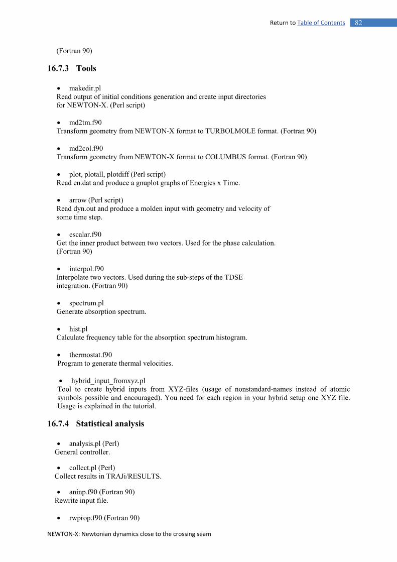
NEWTON-X: Newtonian dynamics close to the crossing seam
82 Return to Table of Contents
(Fortran 90)
16.7.3 Tools
• makedir.pl Read output of initial conditions generation and create input directories for NEWTON-X. (Perl script)
• md2tm.f90 Transform geometry from NEWTON-X format to TURBOLMOLE format. (Fortran 90)
• md2col.f90 Transform geometry from NEWTON-X format to COLUMBUS format. (Fortran 90)
• plot, plotall, plotdiff (Perl script) Read en.dat and produce a gnuplot graphs of Energies x Time.
• arrow (Perl script) Read dyn.out and produce a molden input with geometry and velocity of some time step.
• escalar.f90 Get the inner product between two vectors. Used for the phase calculation. (Fortran 90)
• interpol.f90 Interpolate two vectors. Used during the sub-steps of the TDSE integration. (Fortran 90)
• spectrum.pl Generate absorption spectrum.
• hist.pl Calculate frequency table for the absorption spectrum histogram.
• thermostat.f90 Program to generate thermal velocities. • hybrid_input_fromxyz.pl
Tool to create hybrid inputs from XYZ-files (usage of nonstandard-names instead of atomic symbols possible and encouraged). You need for each region in your hybrid setup one XYZ file. Usage is explained in the tutorial.
16.7.4 Statistical analysis
• analysis.pl (Perl) General controller.
• collect.pl (Perl) Collect results in TRAJi/RESULTS.
• aninp.f90 (Fortran 90) Rewrite input file.
• rwprop.f90 (Fortran 90)

NEWTON-X: Newtonian dynamics close to the crossing seam
83 Return to Table of Contents
Rewrite temporary files to final output format.
• statistics.f90 (Fortran 90) Compute mean value and standard deviation.
• smoothangle.pl (Perl) Corrects discontinuities in angle-values in prop.3.
• splithist.pl (Perl) Splits prop.proptype files in single history-files for each trajectory.
• collectjumps.pl (Perl) Collects information about surface hopping events.
• diagnostic.pl (Perl) Collect information in each trajectory about errors of execution, conservation of energy and conservation of adiabatic population. • run-dftb (Perl) Run DFTB program and read the results.

NEWTON-X: Newtonian dynamics close to the crossing seam
84 Return to Table of Contents
17 Links to third-party programs
COLUMBUS: www.univie.ac.at/columbus TURBOMOLE: www.turbomole.com DFTB and DFTB+: www.dftb.org GAUSSIAN: www.gaussian.com TINKER: dasher.wustl.edu/tinker GAMESS: www.msg.ameslab.gov/gamess

NEWTON-X: Newtonian dynamics close to the crossing seam
85 Return to Table of Contents
18 References
1 M. Barbatti, G. Granucci, M. Persico, M. Ruckenbauer, M. Vazdar, M. Eckert-Maksić, and H. Lischka, J. Photochem. Photobiol., A 190, 228 (2007).
2 M. Barbatti, G. Granucci, M. Ruckenbauer, F. Plasser, R. Crespo-Otero, J. Pittner, M. Persico, and H. Lischka, NEWTON-X: a package for Newtonian dynamics close to the crossing seam, www.newtonx.org (2013).
3 M. Barbatti, M. Ruckenbauer, F. Plasser, J. Pittner, G. Granucci, M. Persico, and H. Lischka, WIREs: Comp. Mol. Sci. 4, 26 (2014).
4 H. Lischka, R. Shepard, R. M. Pitzer, I. Shavitt, M. Dallos, T. Müller, P. G. Szalay, M. Seth, G. S. Kedziora, S. Yabushita, and Z. Y. Zhang, Phys. Chem. Chem. Phys. 3, 664 (2001).
5 H. Lischka, R. Shepard, I. Shavitt, R. M. Pitzer, M. Dallos, T. Müller, P. G. Szalay, F. B. Brown, R. Ahlrichs, H. J. Boehm, A. Chang, D. C. Comeau, R. Gdanitz, H. Dachsel, C. Ehrhardt, M. Ernzerhof, P. Höchtl, S. Irle, G. Kedziora, T. Kovar, V. Parasuk, M. J. M. Pepper, P. Scharf, H. Schiffer, M. Schindler, M. Schüler, M. Seth, E. A. Stahlberg, J.-G. Zhao, S. Yabushita, Z. Zhang, M. Barbatti, S. Matsika, M. Schuurmann, D. R. Yarkony, S. R. Brozell, E. V. Beck, J.-P. Blaudeau, M. Ruckenbauer, B. Sellner, F. Plasser, and J. J. Szymczak, COLUMBUS, an ab initio electronic structure program, release 5.9.2, www.univie.ac.at/columbus (2008).
6 R. Ahlrichs, M. Bär, M. Häser, H. Horn, and C. Kölmel, Chem. Phys. Lett. 162, 165 (1989). 7 M. J. Frisch, G. W. Trucks, H. B. Schlegel, G. E. Scuseria, M. A. Robb, J. R. Cheeseman, J.
Montgomery, J. A., T. Vreven, K. N. Kudin, J. C. Burant, J. M. Millam, S. S. Iyengar, J. Tomasi, V. Barone, B. Mennucci, M. Cossi, G. Scalmani, N. Rega, G. A. Petersson, H. Nakatsuji, M. Hada, M. Ehara, K. Toyota, R. Fukuda, J. Hasegawa, M. Ishida, T. Nakajima, Y. Honda, O. Kitao, H. Nakai, M. Klene, X. Li, J. E. Knox, H. P. Hratchian, J. B. Cross, V. Bakken, C. Adamo, J. Jaramillo, R. Gomperts, R. E. Stratmann, O. Yazyev, A. J. Austin, R. Cammi, C. Pomelli, J. W. Ochterski, P. Y. Ayala, K. Morokuma, G. A. Voth, P. Salvador, J. J. Dannenberg, V. G. Zakrzewski, S. Dapprich, A. D. Daniels, M. C. Strain, O. Farkas, D. K. Malick, A. D. Rabuck, K. Raghavachari, J. B. Foresman, J. V. Ortiz, Q. Cui, A. G. Baboul, S. Clifford, J. Cioslowski, B. B. Stefanov, G. Liu, A. Liashenko, P. Piskorz, I. Komaromi, R. L. Martin, D. J. Fox, T. Keith, M. A. Al-Laham, C. Y. Peng, A. Nanayakkara, M. Challacombe, P. M. W. Gill, B. Johnson, W. Chen, M. W. Wong, C. Gonzalez, and J. A. Pople, Gaussian 03, Revision C.02. Gaussian, Inc., Wallingford CT (2004).
8 M. J. Frisch, G. W. Trucks, H. B. Schlegel, G. E. Scuseria, M. A. Robb, J. R. Cheeseman, G. Scalmani, V. Barone, B. Mennucci, G. A. Petersson, H. Nakatsuji, M. Caricato, X. Li, H. P. Hratchian, A. F. Izmaylov, J. Bloino, G. Zheng, J. L. Sonnenberg, M. Hada, M. Ehara, K. Toyota, R. Fukuda, J. Hasegawa, M. Ishida, T. Nakajima, Y. Honda, O. Kitao, H. Nakai, T. Vreven, J. Montgomery, J. A., J. E. Peralta, F. Ogliaro, M. Bearpark, J. J. Heyd, E. Brothers, K. N. Kudin, V. N. Staroverov, R. Kobayashi, J. Normand, K. Raghavachari, A. Rendell, J. C. Burant, S. S. Iyengar, J. Tomasi, M. Cossi, N. Rega, N. J. Millam, M. Klene, J. E. Knox, J. B. Cross, V. Bakken, C. Adamo, J. Jaramillo, R. Gomperts, R. E. Stratmann, O. Yazyev, A. J. Austin, R. Cammi, C. Pomelli, J. W. Ochterski, R. L. Martin, K. Morokuma, V. G. Zakrzewski, G. A. Voth, P. Salvador, J. J. Dannenberg, S. Dapprich, A. D. Daniels, Ö. Farkas, J. B. Foresman, J. V. Ortiz, J. Cioslowski, and D. J. Fox, Gaussian 09, Revision D.01. Gaussian, Inc., Wallingford CT (2013).
9 M. S. Gordon and M. W. Schmidt, in Theory and Applications of Computational Chemistry the first forty years, edited by C. E. Dykstra, G. Frenking, K. S. Kim, and G. E. Scuseria (Elsevier, Amsterdam, 2005), pp. 1167.
10 M. Elstner, Theor. Chem. Acc. 116, 316 (2006).

NEWTON-X: Newtonian dynamics close to the crossing seam
86 Return to Table of Contents
11 J. W. Ponder and F. M. Richards, J. Comput. Chem. 8, 1016 (1987). 12 J. C. Tully, Faraday Discuss. 110, 407 (1998). 13 J. C. Tully and R. K. Preston, J. Chem. Phys. 55, 562 (1971). 14 J. C. Tully, J. Chem. Phys. 93, 1061 (1990). 15 M. Barbatti, WIREs: Comp. Mol. Sci. 1, 620 (2011). 16 E. Fabiano, G. Groenhof, and W. Thiel, Chem. Phys. 351, 111 (2008). 17 C. Lasser and T. Swart, J. Chem. Phys. 129, 034302 (2008). 18 A. Ferretti, G. Granucci, A. Lami, M. Persico, and G. Villani, J. Chem. Phys. 104, 5517
(1996). 19 J. Pittner, H. Lischka, and M. Barbatti, Chem. Phys. 356, 147 (2009). 20 S. Hammes-Schiffer and J. C. Tully, J. Chem. Phys. 101, 4657 (1994). 21 G. Granucci, M. Persico, and A. Toniolo, J. Chem. Phys. 114, 10608 (2001). 22 E. Tapavicza, I. Tavernelli, and U. Rothlisberger, Phys. Rev. Lett. 98, 023001 (2007). 23 U. Werner, R. Mitrić, T. Suzuki, and V. Bonačić-Koutecký, Chem. Phys. 349, 319 (2008). 24 M. Dallos, H. Lischka, R. Shepard, D. R. Yarkony, and P. G. Szalay, J. Chem. Phys. 120,
7330 (2004). 25 H. Lischka, M. Dallos, P. G. Szalay, D. R. Yarkony, and R. Shepard, J. Chem. Phys. 120,
7322 (2004). 26 C. Y. Zhu, S. Nangia, A. W. Jasper, and D. G. Truhlar, J. Chem. Phys. 121, 7658 (2004). 27 G. Granucci and M. Persico, J. Chem. Phys. 126, 134114 (2007). 28 U. Muller and G. Stock, J. Chem. Phys. 107, 6230 (1997). 29 A. W. Jasper, S. N. Stechmann, and D. G. Truhlar, J. Chem. Phys. 116, 5424 (2002). 30 L. Verlet, Phys. Rev. 159, 98 (1967). 31 W. C. Swope, H. C. Andersen, P. H. Berens, and K. R. Wilson, J. Chem. Phys. 76, 637
(1982). 32 F. Plasser, G. Granucci, J. Pittner, M. Barbatti, M. Persico, and H. Lischka, J. Chem. Phys.
137, 22A514 (2012). 33 T. Atsumi and H. Nakai, J. Chem. Phys. 128 (2008). 34 H. C. Andersen, J. Chem. Phys. 72, 2384 (1980). 35 V. Lukes, R. Solc, M. Barbatti, M. Elstner, H. Lischka, and H.-F. Kauffmann, J. Chem. Phys.
129, 164905 (2008). 36 M. Ruckenbauer, M. Barbatti, T. Muller, and H. Lischka, J. Phys. Chem. A 114, 6757 (2010). 37 S. Grimme and M. Waletzke, J. Chem. Phys. 111, 5645 (1999). 38 B. Sellner, M. Barbatti, and H. Lischka, J. Chem. Phys. 131, 024312 (2009). 39 R. Crespo-Otero and M. Barbatti, Theor. Chem. Acc. 131, 1237 (2012). 40 A. Amadei, A. B. M. Linssen, and H. J. C. Berendsen, Proteins-Structure Function and
Genetics 17, 412 (1993). 41 F. Plasser, M. Barbatti, A. J. A. Aquino, and H. Lischka, J. Phys. Chem. A 113, 8490 (2009). 42 J. P. Dahl and M. Springborg, J. Chem. Phys. 88, 4535 (1988). 43 R. Schinke, Photodissociation Dynamics: Spectroscopy and Fragmentation of Small
Polyatomic Molecules. (Cambridge University Press, Cambridge, 1995). 44 M. Barbatti, A. J. A. Aquino, and H. Lischka, Phys. Chem. Chem. Phys. 12, 4959 (2010). 45 R. C. Hilborn, Am. J. Phys. 50, 982 (1982). 46 J. P. Bergsma, P. H. Berens, K. R. Wilson, D. R. Fredkin, and E. J. Heller, J. Phys. Chem. 88,
612 (1984). 47 J. R. Lakowicz, Principles of fluorescence spectroscopy, 3rd ed. (Springer, Singapore, 2006). 48 E. A. Koopman and C. P. Lowe, J. Chem. Phys. 124 (2006). 49 J. Butcher, J. Assoc. Comp. Mach. 12, 124 (1965). 50 C. F. F. Karney, J. Mol. Graph. Model. 25, 595 (2007).