phylogenetic trees lecture 3 based on: durbin et al 7.4; gusfield 17
Post on 21-Dec-2015
213 views
TRANSCRIPT
.
Phylogenetic Trees
Lecture 3
Based on: Durbin et al 7.4; Gusfield 17
2
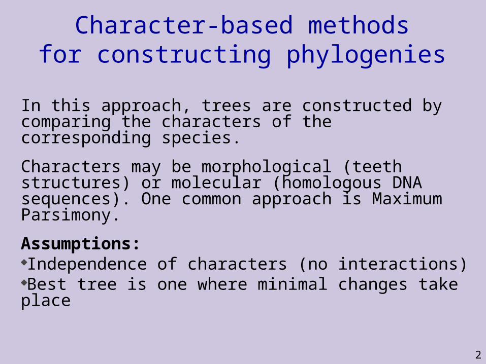
Character-based methodsfor constructing phylogenies
In this approach, trees are constructed by comparing the characters of the corresponding species.
Characters may be morphological (teeth structures) or molecular (homologous DNA sequences). One common approach is Maximum Parsimony.
Assumptions:Independence of characters (no interactions)Best tree is one where minimal changes take place
3
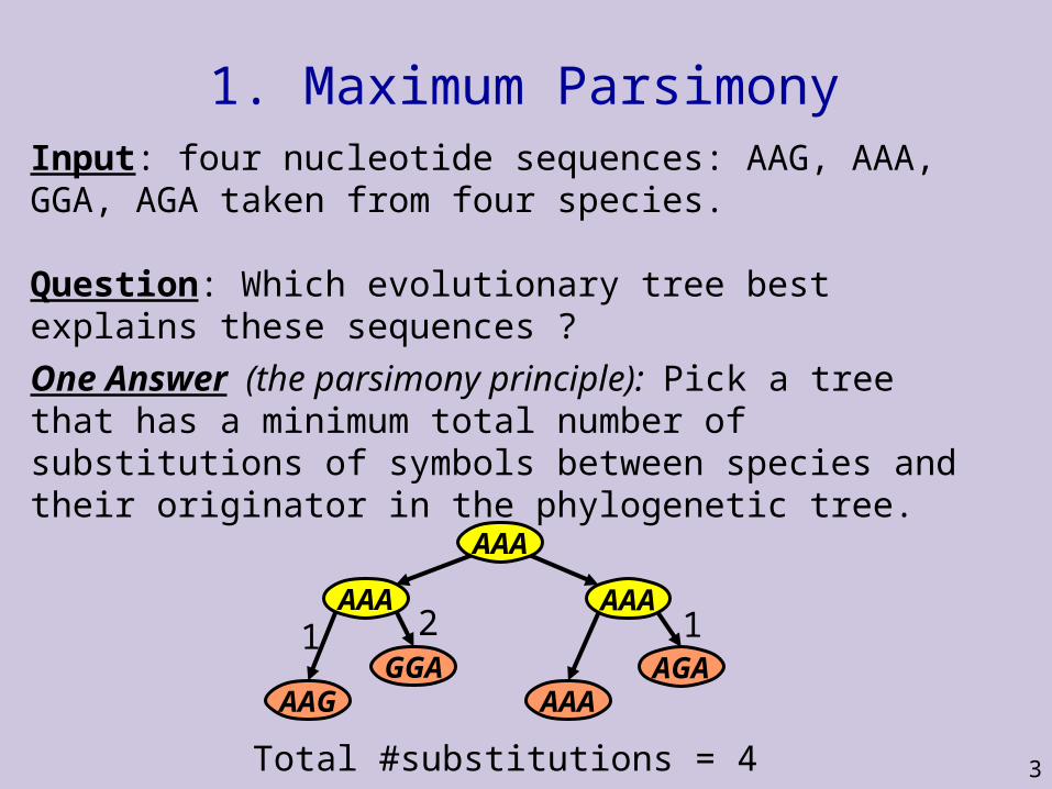
1. Maximum ParsimonyInput: four nucleotide sequences: AAG, AAA, GGA, AGA taken from four species.
Question: Which evolutionary tree best explains these sequences ?
AGAAAA
GGAAAG
AAA AAA
AAA
21 1
Total #substitutions = 4
One Answer (the parsimony principle): Pick a tree that has a minimum total number of substitutions of symbols between species and their originator in the phylogenetic tree.
4
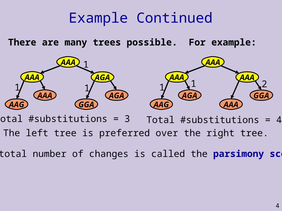
Example Continued
There are many trees possible. For example:
AGAGGA
AAAAAG
AAA AGA
AAA
11
1
Total #substitutions = 3
GGAAAA
AGAAAG
AAA AAA
AAA
11 2
Total #substitutions = 4
The left tree is preferred over the right tree.
The total number of changes is called the parsimony score.
5
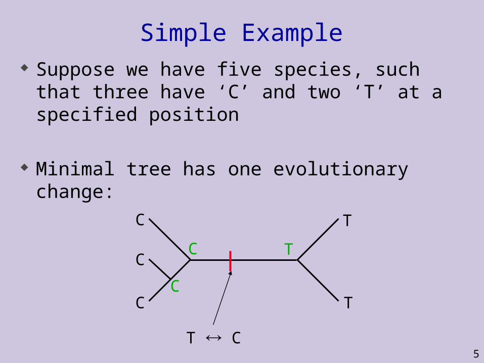
Simple Example Suppose we have five species, such that three
have ‘C’ and two ‘T’ at a specified position
Minimal tree has one evolutionary change:
C
C
CC
C
T
T
T
T C
6
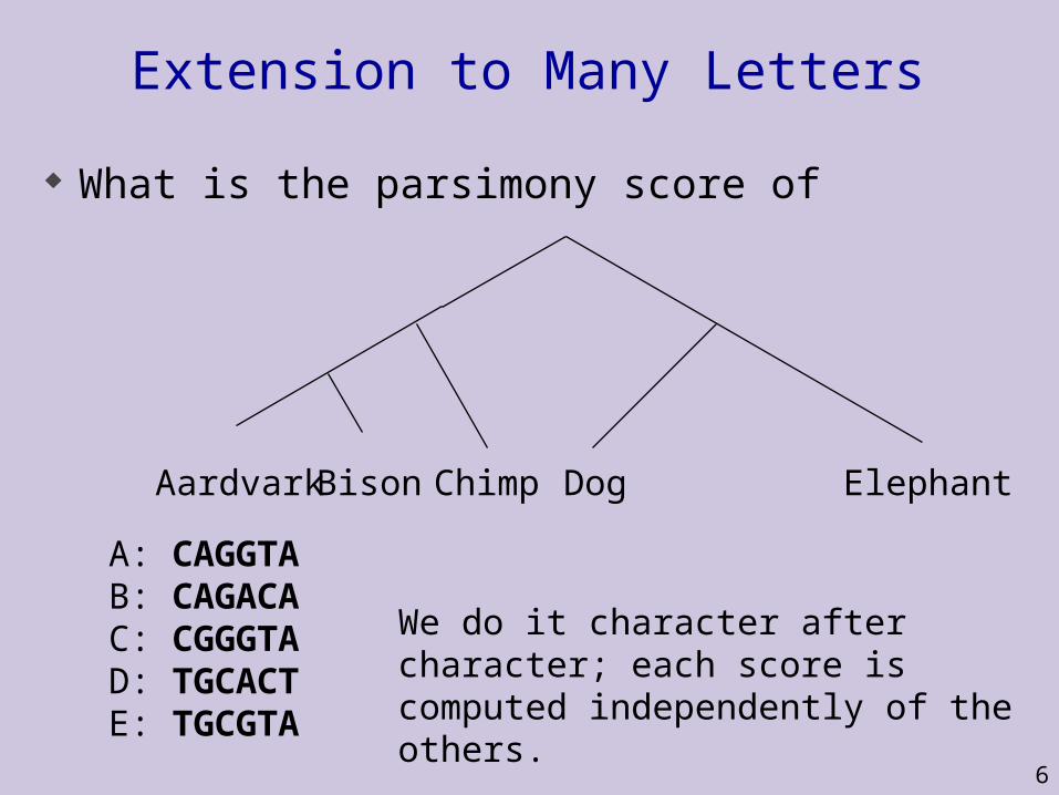
Extension to Many Letters
What is the parsimony score of
Aardvark Bison Chimp Dog Elephant
A: CAGGTAB: CAGACAC: CGGGTAD: TGCACTE: TGCGTA
We do it character after character; each score is computed independently of the others.
7
Fitch’s Algorithm of Evaluating Trees
Traverse tree from leaves to root determining set of possible states (e.g. nucleotides) for each internal node
Traverse tree from root to leaves picking ancestral states for internal nodes
8
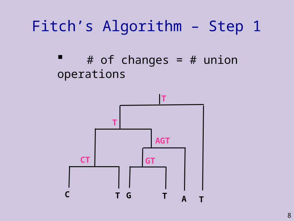
Fitch’s Algorithm – Step 1
# of changes = # union operations
T
T
CT
T
C T AG T
AGT
GT

9
Fitch’s Algorithm – Step 1
Do a post-order (from leaves to root) traversal of tree
Determine possible states Ri of internal node i with children j and k
otherwiseRR
RRifRRR
kj
kjkj
i
10
Fitch’s Algorithm – Step 2
T
T
CT
T
C T AG T
AGT
GT
T
T
CT
T
C T AG T
AGT
GT
T
T
CT
T
C T AG T
AGT
GT
T
T
CT
T
C T AG T
AGT
GT
T
T
CT
T
C T AG T
AGT
GT
T
T
CT
T
C T AG T
AGT
GT
11
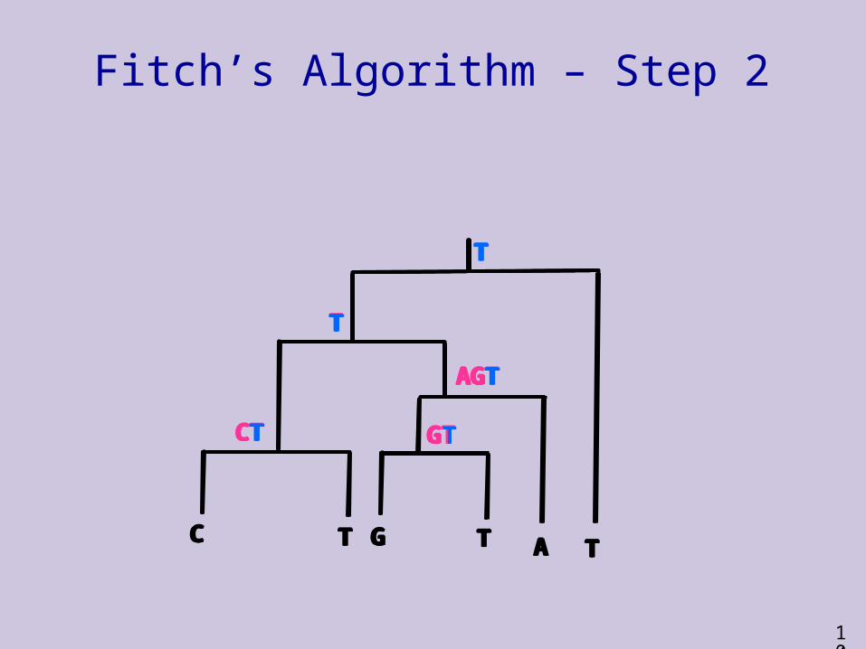
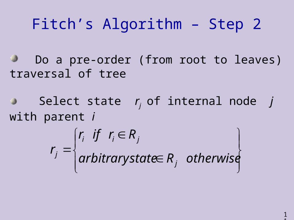
Fitch’s Algorithm – Step 2
Do a pre-order (from root to leaves) traversal of tree
Select state rj of internal node j with parent i
otherwiseRstatearbitrary
Rrifrr
j
jii
j
12
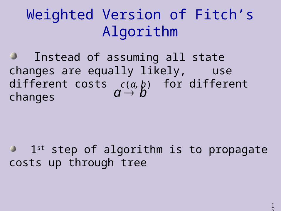
Weighted Version of Fitch’s Algorithm
Instead of assuming all state changes are equally likely, use different costs c(a, b) for different changes
1st step of algorithm is to propagate costs up through tree
ba

13
Weighted Version of Fitch’s Algorithm
Want to determine minimal cost S(i, a)of assigning character a to node i
For leaves:
otherwise
leafatcharacteraisaifS(i, a)
0
14
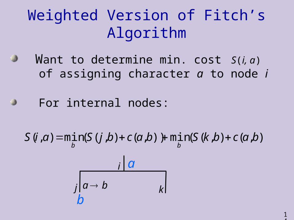
Weighted Version of Fitch’s Algorithm
Want to determine min. cost S(i, a)
of assigning character a to node i
For internal nodes:
)),(),((min)),(),((min),( bacbkSbacbjSaiSbb
a
b
i
j kba
15
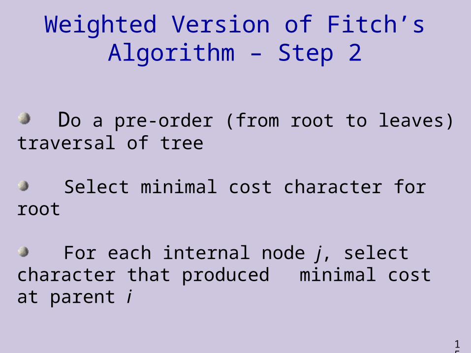
Weighted Version of Fitch’s Algorithm – Step 2
Do a pre-order (from root to leaves) traversal of tree
Select minimal cost character for root
For each internal node j, select character that produced minimal cost at parent i
16
Weighted Parsimony Scores
Weighted Parsimony score:
Each change is weighted by a score c(a, b).
The weighted parsimony score reduces to the parsimony score when c(a,a)=0 and c(a,b)=1 for all b a.
17
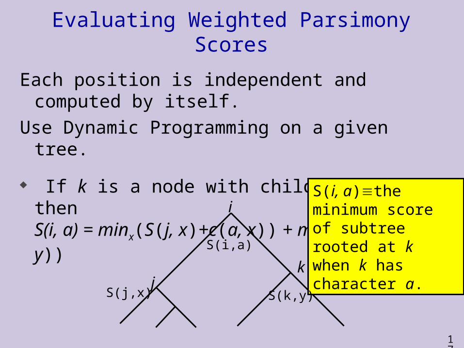
Evaluating Weighted Parsimony Scores
Each position is independent and computed by itself.
Use Dynamic Programming on a given tree.
If k is a node with children i and j, then S(i, a) = minx(S(j, x)+c(a, x)) + miny(S(k, y)+c(a, y))
i
jk
S(j,x)
S(i, a)the minimum score of subtree rooted at k when k has character a.
S(k,y)
S(i,a)
18
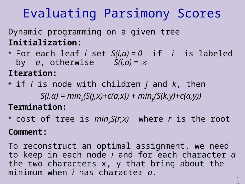
Evaluating Parsimony ScoresDynamic programming on a given treeInitialization: For each leaf i set S(i,a) = 0 if i is labeled by a,
otherwise S(i,a) = Iteration: if i is node with children j and k, then
S(i,a) = minx(S(j,x)+c(a,x)) + miny(S(k,y)+c(a,y))
Termination: cost of tree is minxS(r,x) where r is the rootComment:
To reconstruct an optimal assignment, we need to keep in each node i and for each character a the two characters x, y that bring about the minimum when i has character a.
19
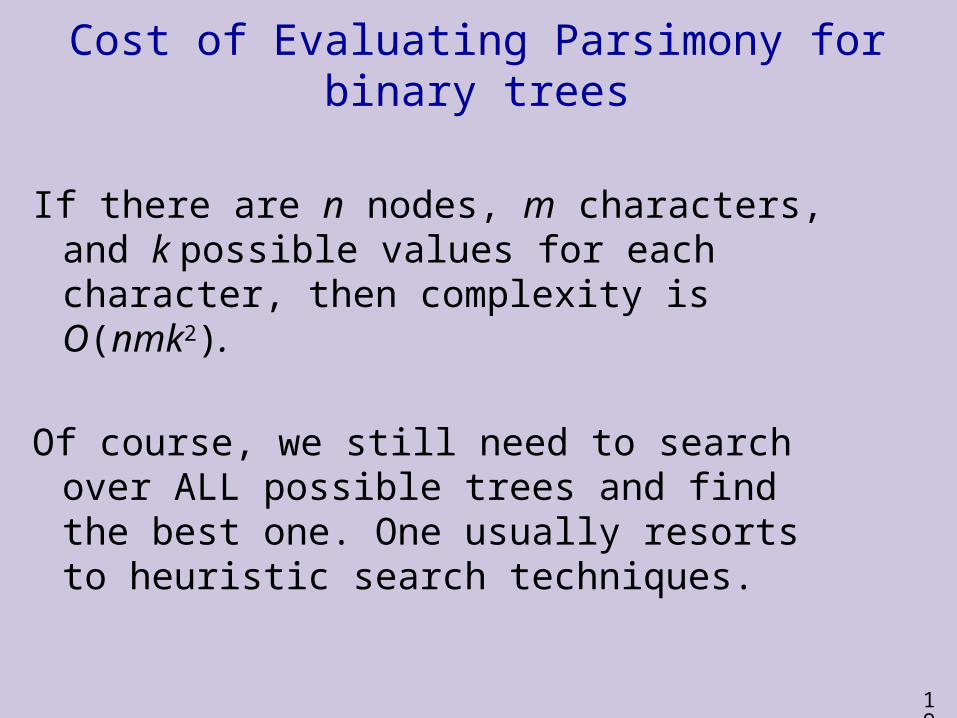
Cost of Evaluating Parsimony for binary trees
If there are n nodes, m characters, and k possible values for each character, then complexity is O(nmk2).
Of course, we still need to search over ALL possible trees and find the best one. One usually resorts to heuristic search techniques.
20
Exploring the Space of Trees
!)!32( n
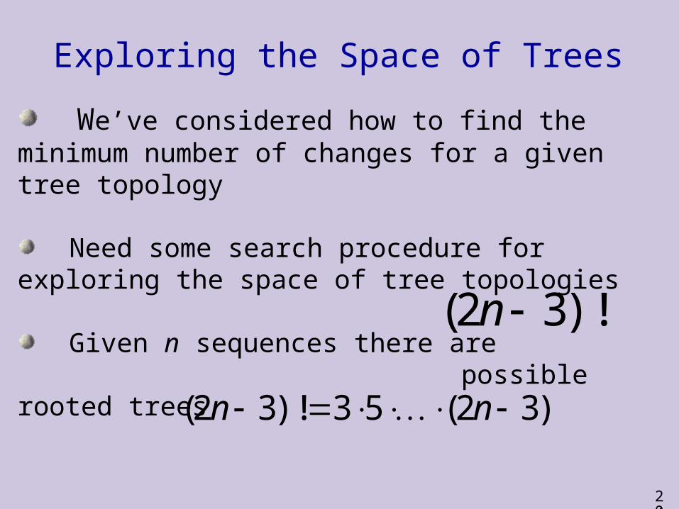
We’ve considered how to find the minimum number of changes for a given tree topology
Need some search procedure for exploring the space of tree topologies
Given n sequences there are possible rooted trees
)32(53!)!32( nn
21
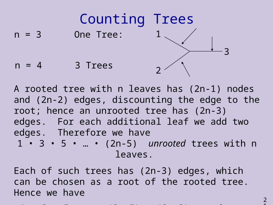
Counting Treesn = 3 One Tree:
n = 4 3 Trees
1
2
3
A rooted tree with n leaves has (2n-1) nodes and (2n-2) edges, discounting the edge to the root; hence an unrooted tree has (2n-3) edges. For each additional leaf we add two edges. Therefore we have
1 • 3 • 5 • … • (2n-5) unrooted trees with n leaves.
Each of such trees has (2n-3) edges, which can be chosen as a root of the rooted tree. Hence we have
1 • 3 • 5 • … • (2n-5) • (2n-3) rooted trees with n leaves
22
Exploring the Space of Trees
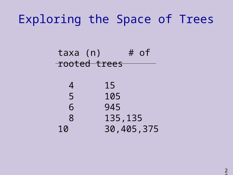
taxa (n) # of rooted trees
4 15 5 105 6 945 8 135,13510 30,405,375
23
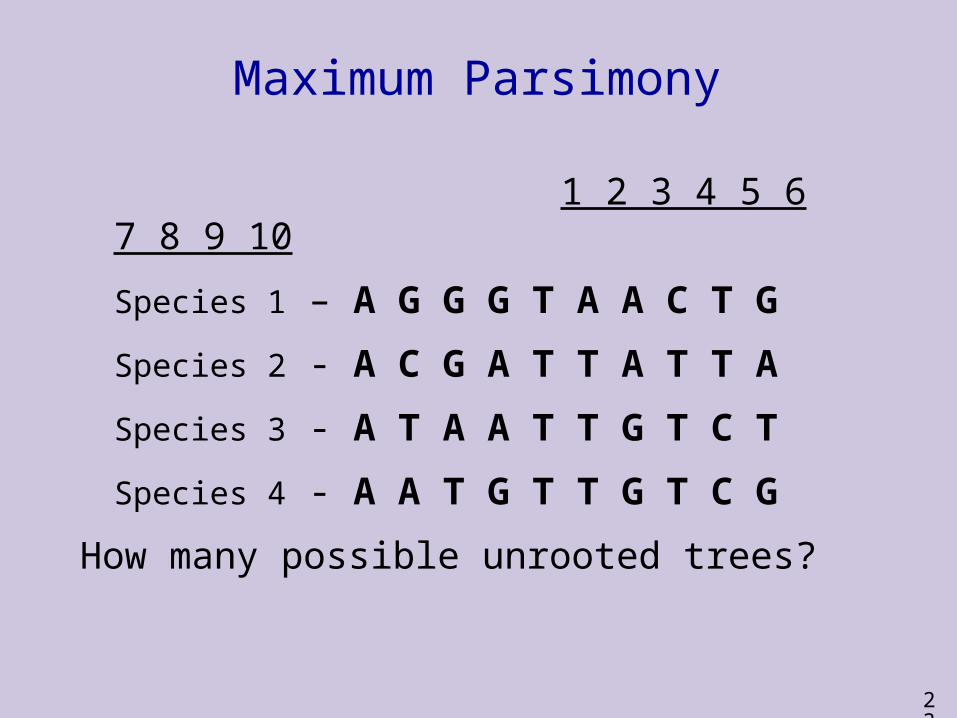
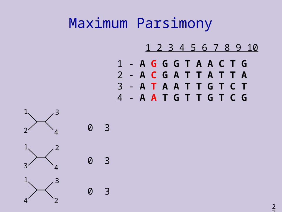
Maximum Parsimony
1 2 3 4 5 6 7 8 9 10
Species 1 – A G G G T A A C T G
Species 2 - A C G A T T A T T A
Species 3 - A T A A T T G T C T
Species 4 - A A T G T T G T C G
How many possible unrooted trees?
24
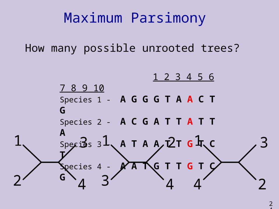
Maximum Parsimony
How many possible unrooted trees?
1
3
2
4
1
2
3
4
1
4
3
2
1 2 3 4 5 6 7 8 9 10Species 1 - A G G G T A A C T GSpecies 2 - A C G A T T A T T ASpecies 3 - A T A A T T G T C TSpecies 4 - A A T G T T G T C G
25
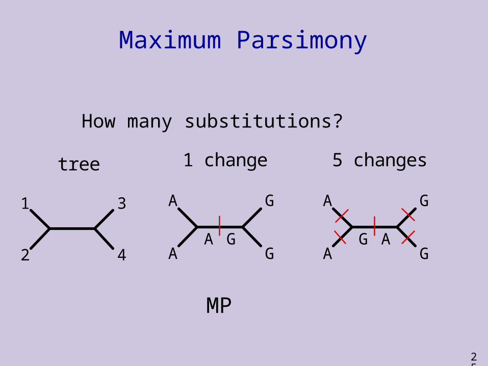
Maximum Parsimony
How many substitutions?
A
A
G
GA G
1 change
A
A
G
GG A
5 changes
1
2
3
4
tree
MP
26
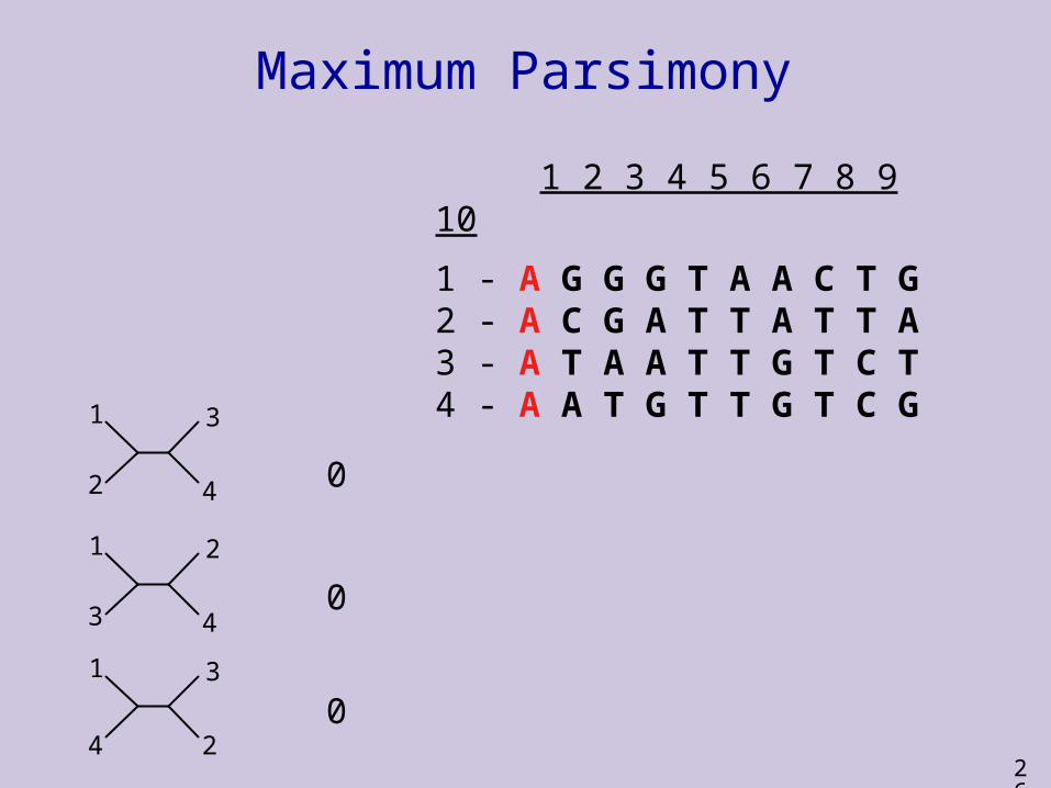
Maximum Parsimony
1 2 3 4 5 6 7 8 9 10
1 - A G G G T A A C T G2 - A C G A T T A T T A3 - A T A A T T G T C T4 - A A T G T T G T C G
0
0
0
1
3
2
4
1
2
3
4
1
4
3
2
27
Maximum Parsimony
1 2 3 4 5 6 7 8 9 10
1 - A G G G T A A C T G2 - A C G A T T A T T A3 - A T A A T T G T C T4 - A A T G T T G T C G
0 3
0 3
0 3
1
3
2
4
1
2
3
4
1
4
3
2
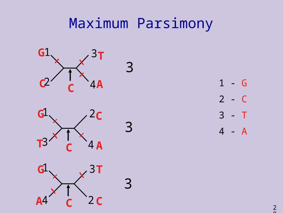
28
Maximum Parsimony
1 - G
2 - C
3 - T
4 - A
1
2
3
4A
G
C
T
C
A
G
T
C1
3
2
4C
C
G
A
T1
4
3
2C
3
3
3

29
Maximum Parsimony
1 2 3 4 5 6 7 8 9 10
1 - A G G G T A A C T G2 - A C G A T T A T T A3 - A T A A T T G T C T4 - A A T G T T G T C G
0 3 2
0 3 2
0 3 2
1
3
2
4
1
2
3
4
1
4
3
2
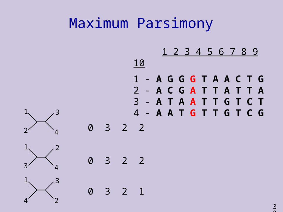
30
Maximum Parsimony
1 2 3 4 5 6 7 8 9 10
1 - A G G G T A A C T G2 - A C G A T T A T T A3 - A T A A T T G T C T4 - A A T G T T G T C G
0 3 2 2
0 3 2 1
0 3 2 2
1
3
2
4
1
2
3
4
1
4
3
2
31
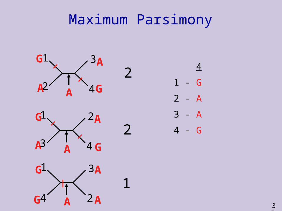
Maximum Parsimony
4
1 - G
2 - A
3 - A
4 - G
1
2
3
4G
G
A
A
A
G
G
A
A1
3
2
4A
AG
G A1
4
3
2A
2
2
1
32
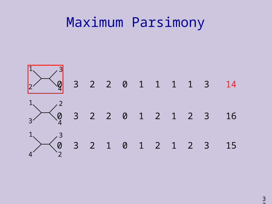
Maximum Parsimony
0 3 2 2 0 1 1 1 1 3 14
0 3 2 1 0 1 2 1 2 3 15
0 3 2 2 0 1 2 1 2 3 16
1
3
2
4
1
2
3
4
1
4
3
2
33
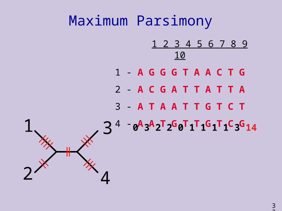
Maximum Parsimony
0 3 2 2 0 1 1 1 1 3 14
1
2
3
4
1 2 3 4 5 6 7 8 9 10
1 - A G G G T A A C T G
2 - A C G A T T A T T A
3 - A T A A T T G T C T
4 - A A T G T T G T C G
34
Finding most parsimonious trees - exact solutions
Exact solutions can only be used for small numbers of taxa.
Exhaustive search examines all possible trees.
Typically used for problems with less than 10 taxa.
35
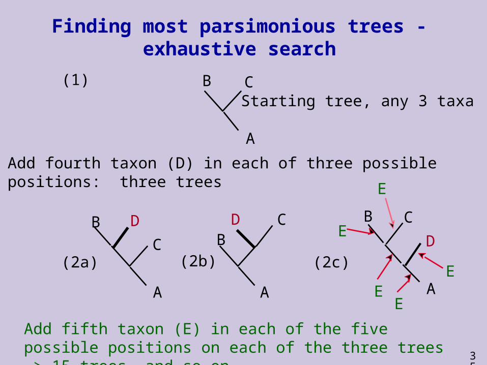
Finding most parsimonious trees - exhaustive search
A
B C(1)
(2a)
Starting tree, any 3 taxa
A
B D
C
A
BD C
(2b) (2c)
E
A
B C
DE
EE
E
Add fourth taxon (D) in each of three possible positions: three trees
Add fifth taxon (E) in each of the five possible positions on each of the three trees -> 15 trees, and so on
36
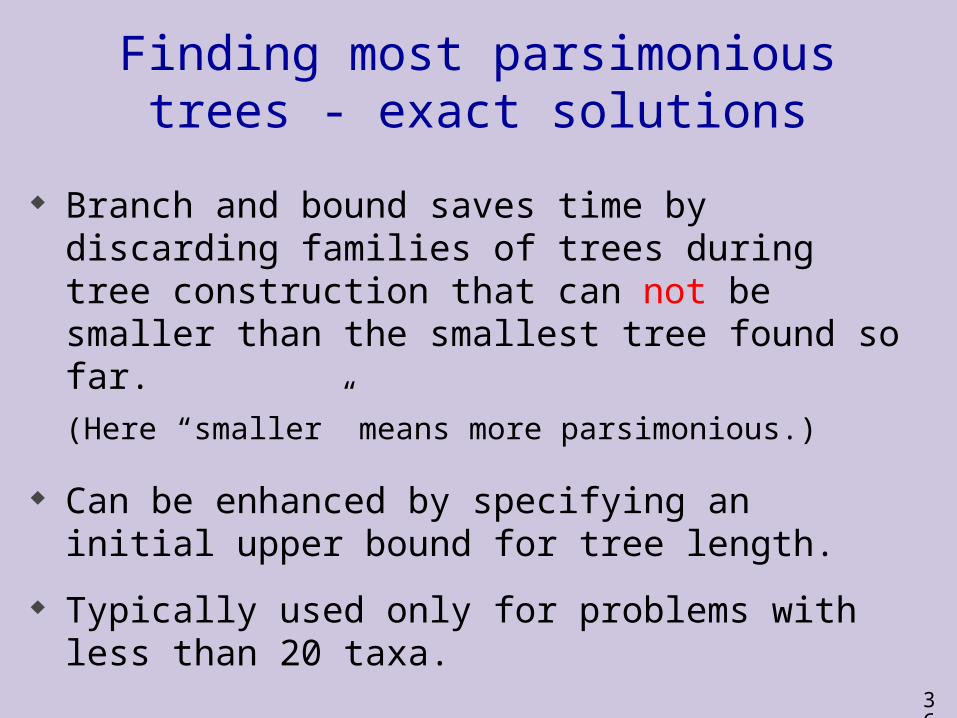
Finding most parsimonious trees - exact solutions
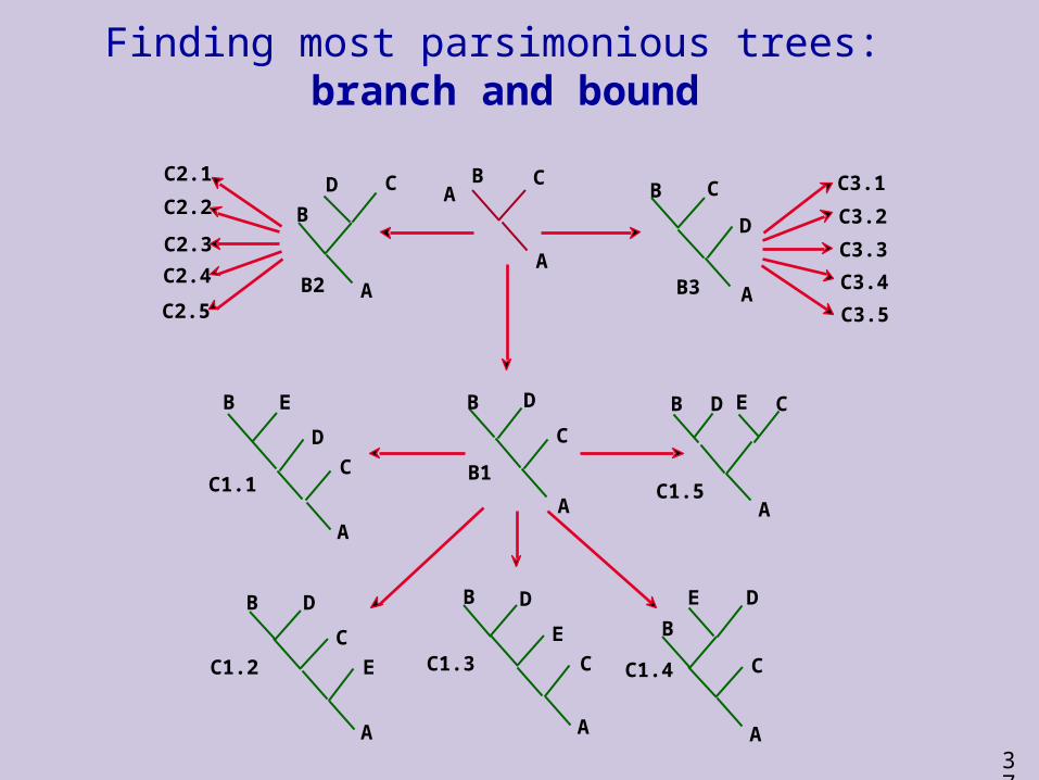
Branch and bound saves time by discarding families of trees during tree construction that can not be smaller than the smallest tree found so far.
(Here “smaller” means more parsimonious.)
Can be enhanced by specifying an initial upper bound for tree length.
Typically used only for problems with less than 20 taxa.
37
Finding most parsimonious trees: branch and bound
A
B C
B1
A
B D
C
A
B C
D
B3
A
A
B E
D
CC1.1
A
B D
E
CC1.3
A
B D
C
EC1.2
A
B
CC1.4
E D
A
B C
C1.5
ED
A
B
D C
B2
C2.1
C2.2
C2.3
C2.4
C2.5
C3.1
C3.2
C3.3
C3.4
C3.5
38
Finding most parsimonious trees - heuristics
The number of possible trees increases exponentially with the number of taxa making exhaustive searches impractical for many data sets (an NP complete problem)
Heuristic methods are used to search tree space for most parsimonious trees
The trees found are not guaranteed to be the most parsimonious - they are best guesses

39
Finding most parsimonious trees - heuristics
Stepwise addition Asis - the order in the data matrix Closest -starts with shortest 3-taxon tree adds taxa in
order that produces the least increase in tree length Simple - the first taxon in the matrix is a taken as a
reference - taxa are added to it in the order of their decreasing similarity to the reference
Random - taxa are added in a random sequence, many different sequences can be used
Recommend random with as many (e.g. 10-100) addition sequences as practical
40
Finding most parsimonious trees - heuristics
Branch Swapping:
Nearest neighbor interchange (NNI)
Subtree pruning and regrafting (SPR)
Tree bisection and reconnection (TBR)
41
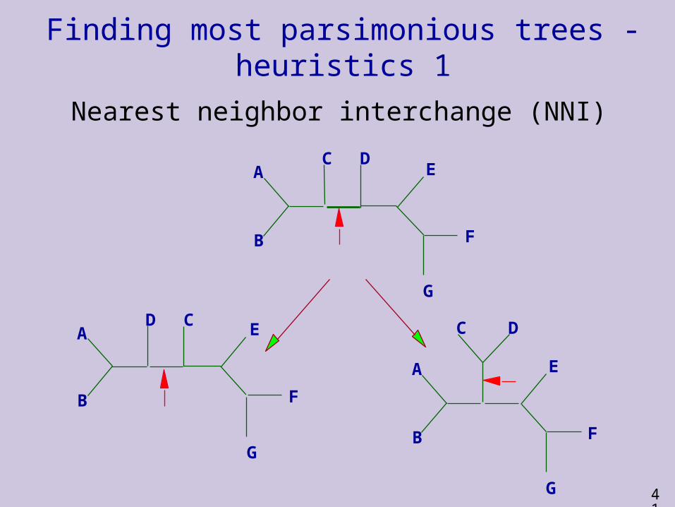
Finding most parsimonious trees - heuristics 1
Nearest neighbor interchange (NNI)
A
B
C DE
F
G
A
B
D CE
F
G
A
B
C D
E
F
G
42
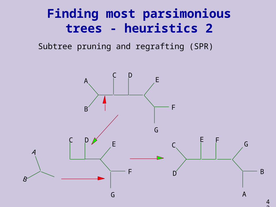
Finding most parsimonious trees - heuristics 2
Subtree pruning and regrafting (SPR)
A
B
C DE
F
G
A
B
C DE
F
G
C
D
G
B
A
E F
43
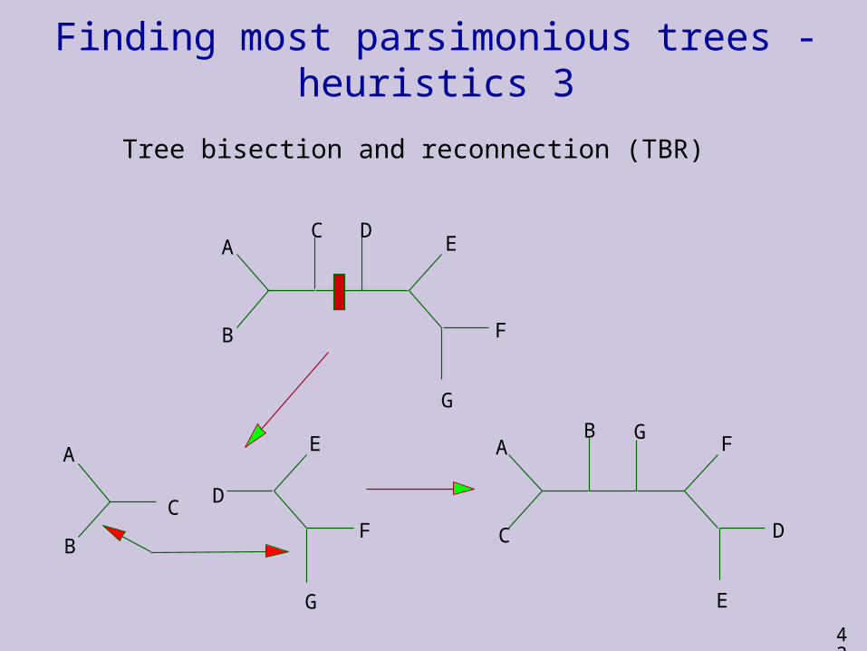
Finding most parsimonious trees - heuristics 3
Tree bisection and reconnection (TBR)
A
B
C DE
F
G
A
B
CD
E
F
G
A
C
F
D
E
B G
44
Finding most parsimonious trees - heuristics - summary
Branch Swapping Nearest neighbor interchange (NNI) Subtree pruning and regrafting (SPR) Tree bisection and reconnection (TBR) The nature of heuristic searches means we cannot
know which method will find the most parsimonious trees or all such trees.
However, TBR is the most extensive swapping routine and its use with multiple random addition sequences should work well.
45
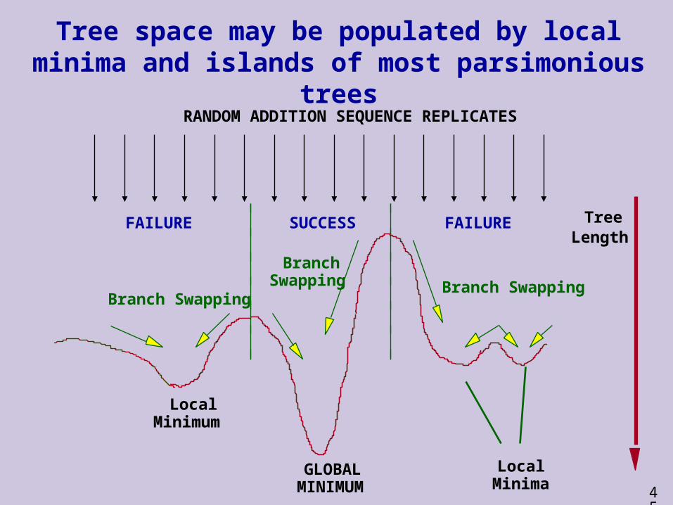
Tree space may be populated by local minima and islands of most parsimonious trees
GLOBAL MINIMUM
LocalMinimum
LocalMinima
TreeLength
RANDOM ADDITION SEQUENCE REPLICATES
SUCCESSFAILURE FAILURE
Branch SwappingBranch Swapping
Branch Swapping
46
Multiple most parsimonious trees
Many parsimony analyses yield multiple equally optimal trees Multiple trees are due to either:
- Alternative equally parsimonious optimizations of homoplastic characters
- Missing data- Or both
We can further select among these trees with additional criteria, but
Most commonly relationships common to all the optimal trees are summarized with consensus trees
47
Consensus methods - 1
A consensus tree is a summary of the agreement among a set of fundamental trees
There are many different consensus methods that differ in:
1. the kind of agreement 2. the level of agreement Consensus methods can be used with any types of
tree - not just parsimony
48
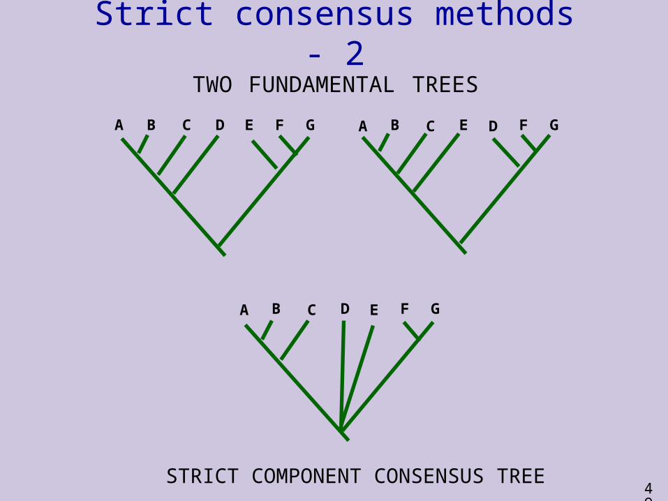
Strict consensus methods - 1 Strict consensus methods require agreement
across all the fundamental trees They show only those relationships that are
unambiguously supported by the parsimonious interpretation of the data
The commonest method (strict component consensus) focuses on clades
This method produces a consensus tree that includes all and only those clades found in all the fundamental trees
Other relationships (those in which the fundamental trees disagree) are shown as unresolved polytomies
49
Strict consensus methods - 2
A B C D E F G A B C E D F G
TWO FUNDAMENTAL TREES
A B C D E F G
STRICT COMPONENT CONSENSUS TREE
50
Majority-rule consensus methods
Majority-rule consensus methods require agreement across a majority of the fundamental trees
May include relationships that are not supported by the most parsimonious interpretation of the data
The commonest method focuses on clades This method produces a consensus tree that
includes all and only those clades found in a majority (>50%) of the fundamental trees
Other relationships are shown as unresolved polytomies
Of particular use in bootstrapping
51
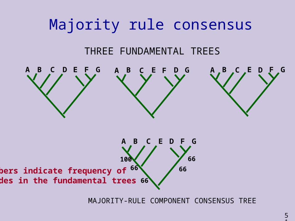
Majority rule consensus
A B C D E F G A B C E D F G
A B C E D F G
MAJORITY-RULE COMPONENT CONSENSUS TREE
A B C E F D G
10066
66
66
66
THREE FUNDAMENTAL TREES
Numbers indicate frequency ofclades in the fundamental trees
52
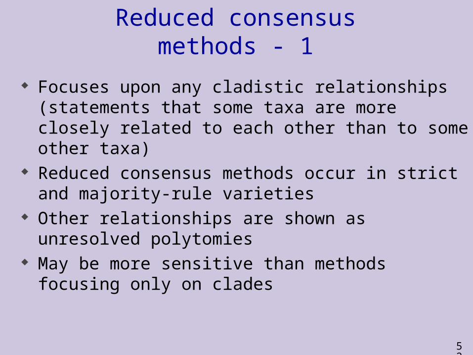
Reduced consensus methods - 1
Focuses upon any cladistic relationships (statements that some taxa are more closely related to each other than to some other taxa)
Reduced consensus methods occur in strict and majority-rule varieties
Other relationships are shown as unresolved polytomies
May be more sensitive than methods focusing only on clades
53
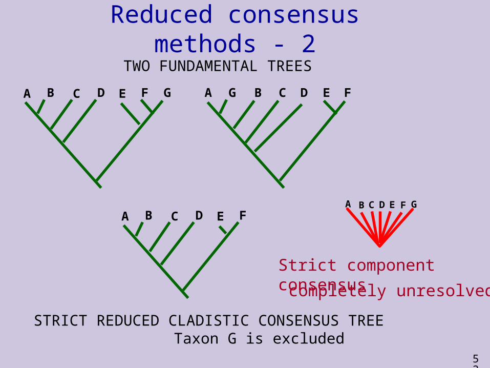
Reduced consensus methods - 2
A B C D E F G
TWO FUNDAMENTAL TREES
STRICT REDUCED CLADISTIC CONSENSUS TREE Taxon G is excluded
A G B C D E F
A B C D E FA B C D E F G
Strict component consensus
completely unresolved
54
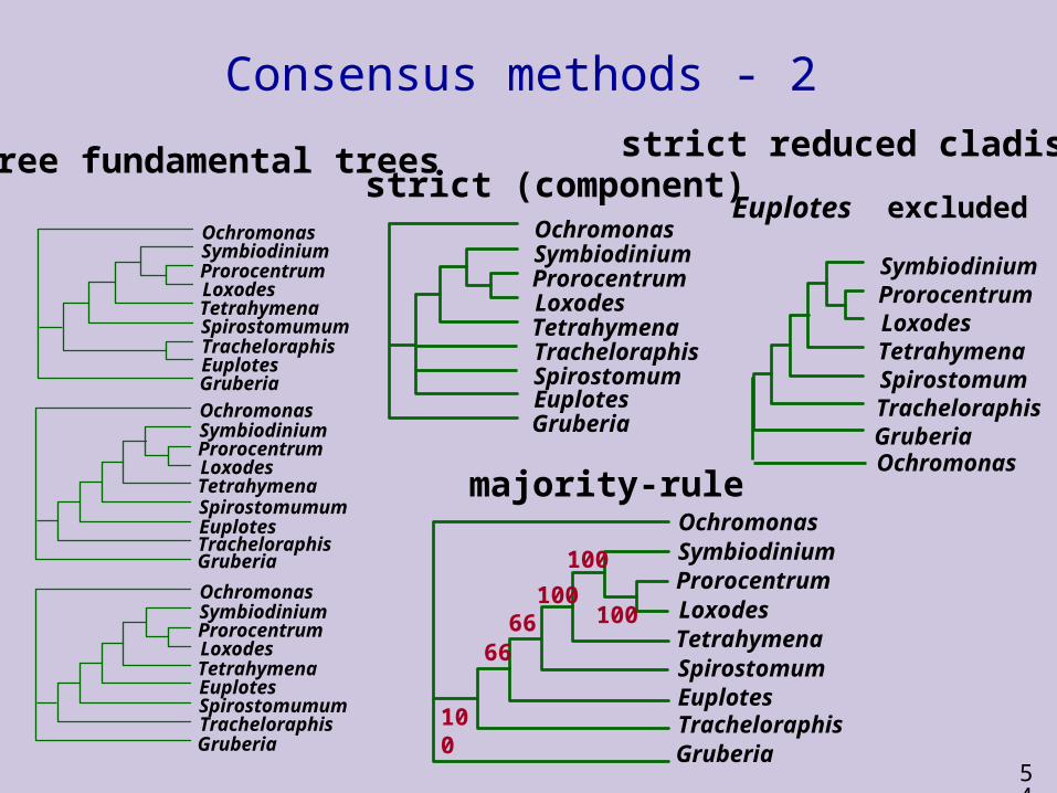
Consensus methods - 2
Spirostomumum
OchromonasSymbiodiniumProrocentrumLoxodesTetrahymena
TracheloraphisEuplotesGruberia
OchromonasSymbiodiniumProrocentrumLoxodesTetrahymenaSpirostomumumEuplotesTracheloraphisGruberia
OchromonasSymbiodiniumProrocentrumLoxodesTetrahymenaEuplotesSpirostomumumTracheloraphisGruberia
OchromonasSymbiodiniumProrocentrumLoxodesTetrahymenaTracheloraphisSpirostomumEuplotesGruberia
OchromonasSymbiodiniumProrocentrumLoxodesTetrahymenaSpirostomumEuplotesTracheloraphisGruberia
Ochromonas
SymbiodiniumProrocentrumLoxodesTetrahymenaSpirostomumTracheloraphisGruberia
Three fundamental trees
majority-rule
strict (component)strict reduced cladistic
Euplotes excluded
100
100100
100
6666

55
Consensus methods - 3 Use strict methods to identify those
relationships unambiguously supported by parsimonious interpretation of the data
Use reduced methods where consensus trees are poorly resolved
Use majority-rule methods in bootstrapping Avoid other methods which have ambiguous
interpretations
56
Parsimony - advantages
a simple method - easily understood operation does not seem to depend on an explicit model of
evolution gives both trees and associated hypotheses of
character evolution should give reliable results if the data is well
structured and homoplasy is either rare or randomly distributed on the tree
57
Parsimony - disadvantages May give misleading results if homoplasy is common or
concentrated in particular parts of the tree, e.g:- thermophilic convergence- base composition biases- long branch attraction
Underestimates branch lengths Model of evolution is implicit - behaviour of method not well
understood Parsimony often justified on purely philosophical grounds - we
must prefer simplest hypotheses - particularly by morphologists
For most molecular systematists this is uncompelling
58
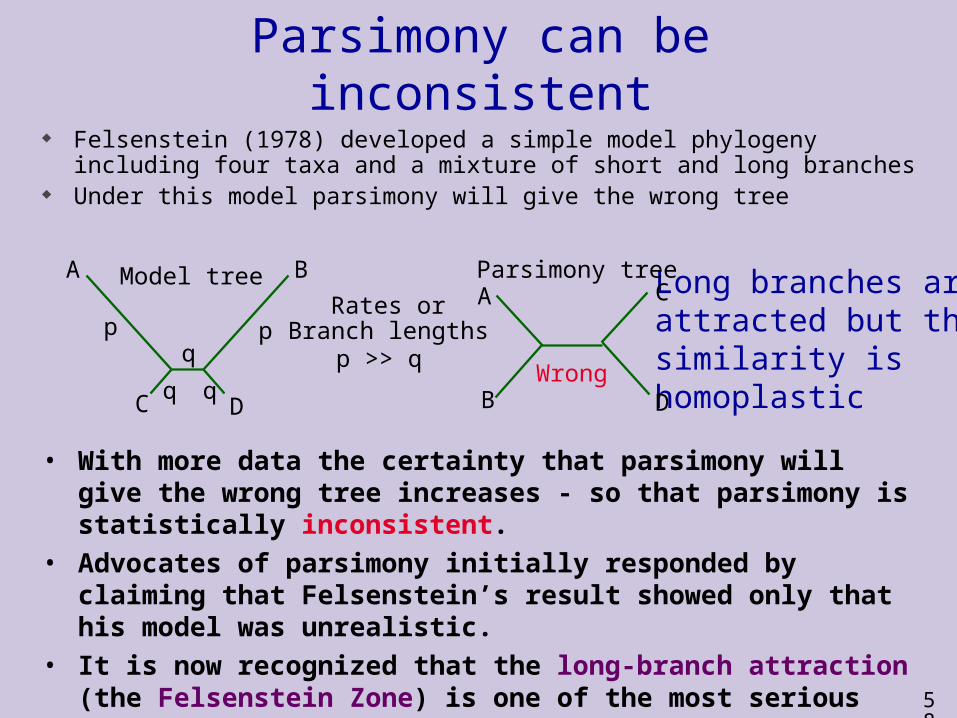
Parsimony can be inconsistent Felsenstein (1978) developed a simple model phylogeny including four
taxa and a mixture of short and long branches Under this model parsimony will give the wrong tree
• With more data the certainty that parsimony will give the wrong tree increases - so that parsimony is statistically inconsistent.
• Advocates of parsimony initially responded by claiming that Felsenstein’s result showed only that his model was unrealistic.
• It is now recognized that the long-branch attraction (the Felsenstein Zone) is one of the most serious problems in phylogenetic inference.
Long branches are attracted but the similarity is homoplastic
A B
C D
Model tree
p pq
q q
Rates or Branch lengths
p >> q
A
B
C
D
Parsimony tree
Wrong
59
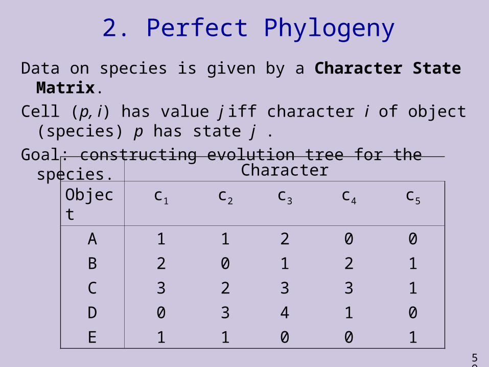
2. Perfect Phylogeny
Data on species is given by a Character State Matrix.
Cell (p, i) has value j iff character i of object (species) p has state j .
Goal: constructing evolution tree for the species.
Character
Object c1 c2 c3 c4 c5
A 1 1 2 0 0
B 2 0 1 2 1
C 3 2 3 3 1
D 0 3 4 1 0
E 1 1 0 0 1
60
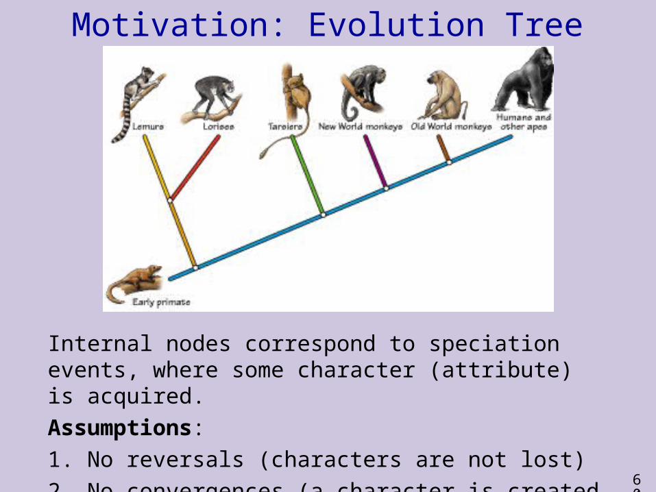
Motivation: Evolution Tree
Internal nodes correspond to speciation events, where some character (attribute) is acquired.Assumptions: 1. No reversals (characters are not lost)2. No convergences (a character is created only once)
61
62
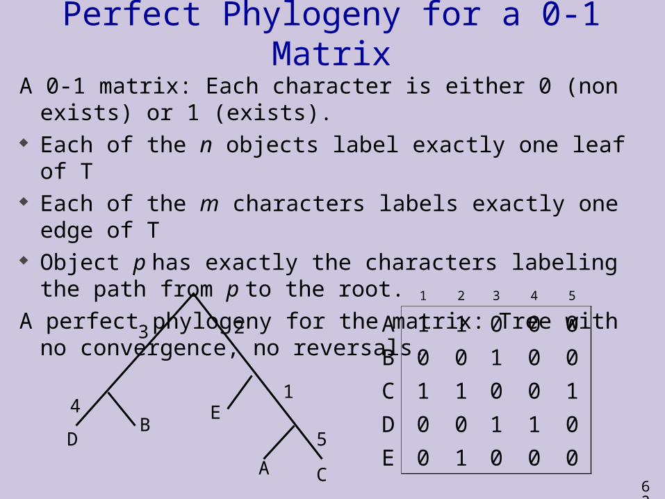
Perfect Phylogeny for a 0-1 Matrix
A 0-1 matrix: Each character is either 0 (non exists) or 1 (exists). Each of the n objects label exactly one leaf of T Each of the m characters labels exactly one edge of T Object p has exactly the characters labeling the path from p to the
root.
A perfect phylogeny for the matrix: Tree with no convergence, no reversals.
1 2 3 4 5
A 1 1 0 0 0
B 0 0 1 0 0
C 1 1 0 0 1
D 0 0 1 1 0
E 0 1 0 0 0A
E
D
C
B4
3 2
1
5
63
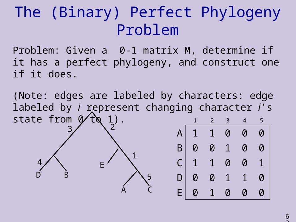
The (Binary) Perfect Phylogeny Problem
Problem: Given a 0-1 matrix M, determine if it has a perfect phylogeny, and construct one if it does.
(Note: edges are labeled by characters: edge labeled by i represent changing character i’s state from 0 to 1).
1 2 3 4 5
A 1 1 0 0 0
B 0 0 1 0 0
C 1 1 0 0 1
D 0 0 1 1 0
E 0 1 0 0 0A
ED
C
B
4
3 2
1
5
64
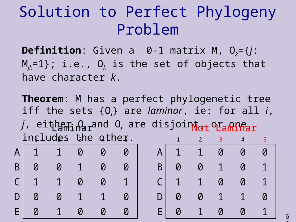
Solution to Perfect Phylogeny Problem
Definition: Given a 0-1 matrix M, Ok={j: Mjk=1}; i.e., Ok is the set of objects that have character k.
Theorem: M has a perfect phylogenetic tree iff the sets {Oi} are laminar, ie: for all i, j, either Oi and Oj are disjoint, or one includes the other.
1 2 3 4 5
A 1 1 0 0 0
B 0 0 1 0 0
C 1 1 0 0 1
D 0 0 1 1 0
E 0 1 0 0 0
1 2 3 4 5
A 1 1 0 0 0
B 0 0 1 0 1
C 1 1 0 0 1
D 0 0 1 1 0
E 0 1 0 0 1
Laminar Not Laminar
65
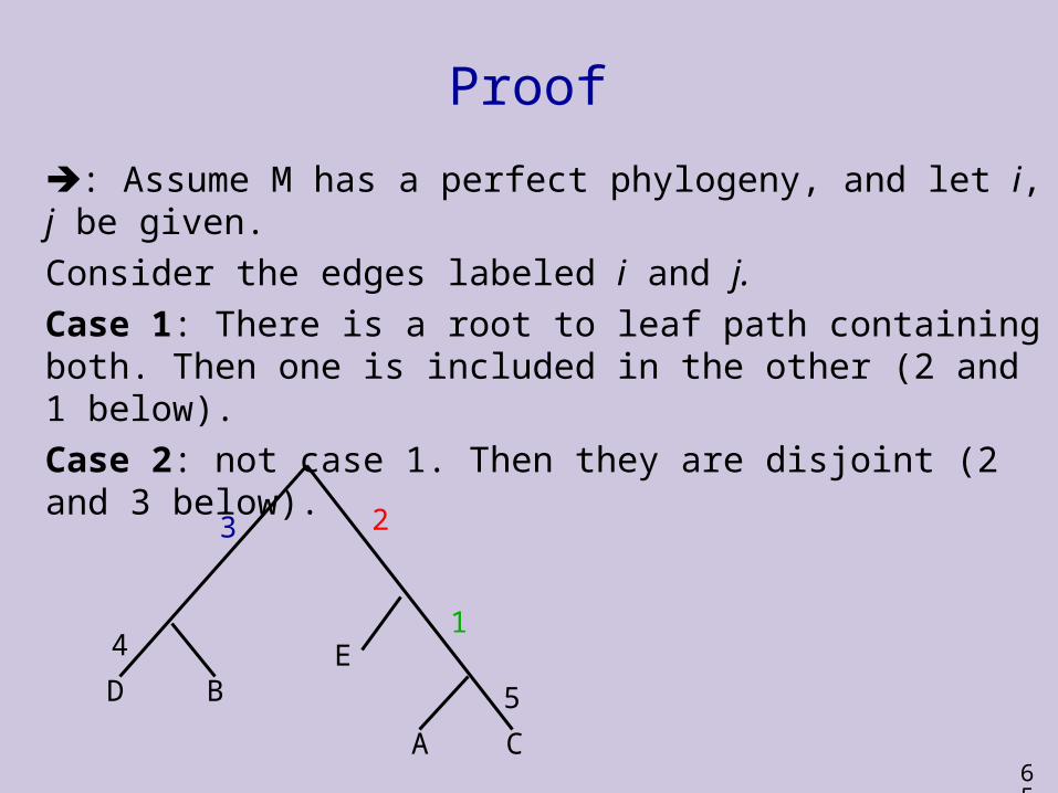
Proof
: Assume M has a perfect phylogeny, and let i, j be given.
Consider the edges labeled i and j.
Case 1: There is a root to leaf path containing both. Then one is included in the other (2 and 1 below).
Case 2: not case 1. Then they are disjoint (2 and 3 below).
A
ED
C
B
4
3 2
1
5
66
Proof (cont.)
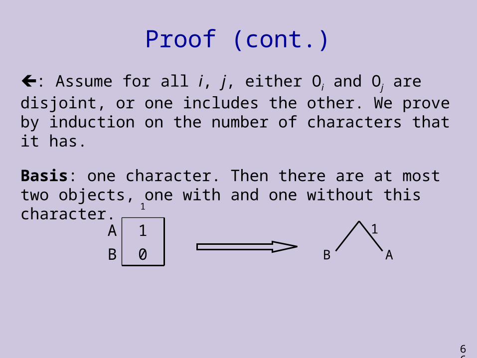
: Assume for all i, j, either Oi and Oj are disjoint, or one includes the other. We prove by induction on the number of characters that it has.
Basis: one character. Then there are at most two objects, one with and one without this character.
0B
1A
1
1
AB
67
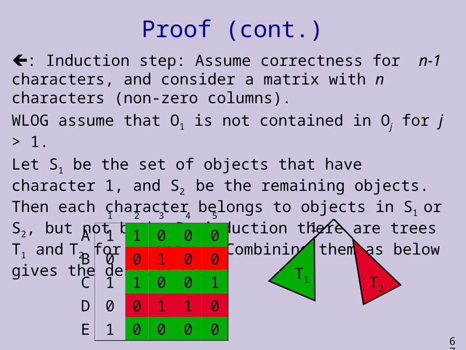
Proof (cont.): Induction step: Assume correctness for n-1 characters, and consider a matrix with n characters (non-zero columns).
WLOG assume that O1 is not contained in Oj for j > 1.
Let S1 be the set of objects that have character 1, and S2 be the remaining objects. Then each character belongs to objects in S1 or S2, but not both. By induction there are trees T1 and T2 for S1 and S2. Combining them as below gives the desired tree.
1 2 3 4 5
A 1 1 0 0 0
B 0 0 1 0 0
C 1 1 0 0 1
D 0 0 1 1 0
E 1 0 0 0 0
T1 T2
1
68
Efficient Implementation
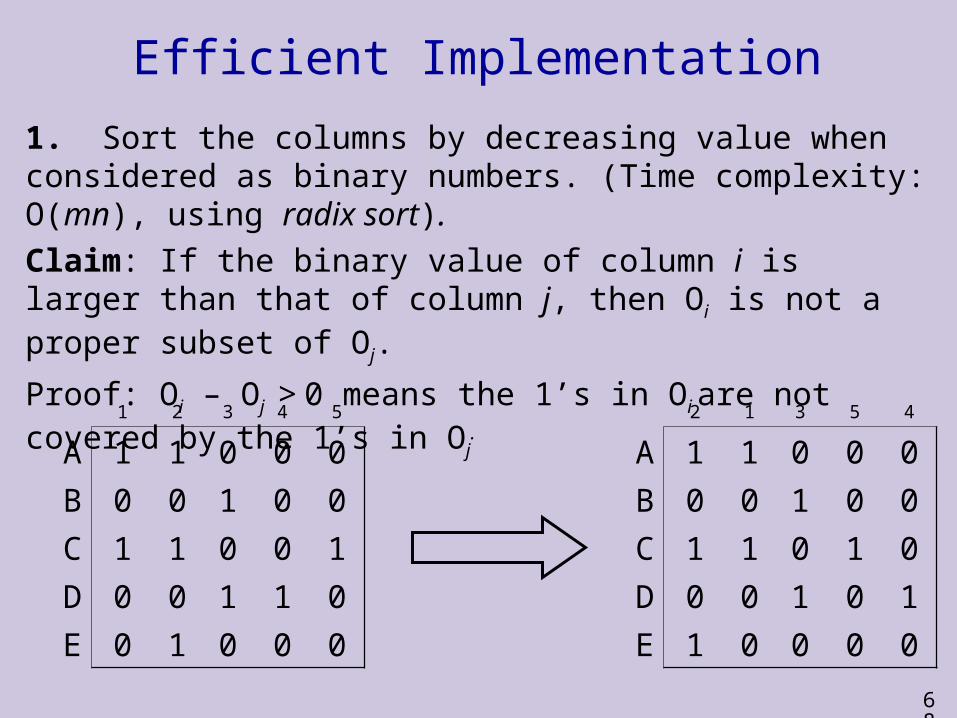
1. Sort the columns by decreasing value when considered as binary numbers. (Time complexity: O(mn), using radix sort).
Claim: If the binary value of column i is larger than that of column j, then Oi is not a proper subset of Oj.
Proof: Oi – Oj > 0 means the 1’s in Oi are not covered by the 1’s in Oj.
1 2 3 4 5
A 1 1 0 0 0
B 0 0 1 0 0
C 1 1 0 0 1
D 0 0 1 1 0
E 0 1 0 0 0
2 1 3 5 4
A 1 1 0 0 0
B 0 0 1 0 0
C 1 1 0 1 0
D 0 0 1 0 1
E 1 0 0 0 0
69
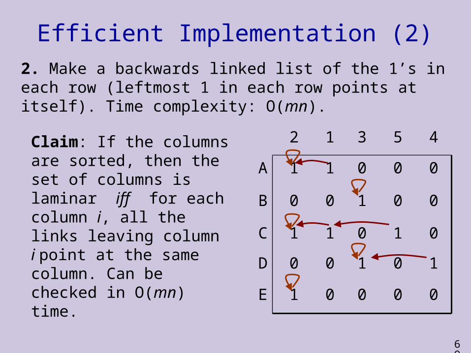
Efficient Implementation (2)2. Make a backwards linked list of the 1’s in each row (leftmost 1 in each row points at itself). Time complexity: O(mn).
00001E
10100D
01011C
00100B
00011A
45312Claim: If the columns are sorted, then the set of columns is laminar iff for each column i, all the links leaving column i point at the same column. Can be checked in O(mn) time.
70
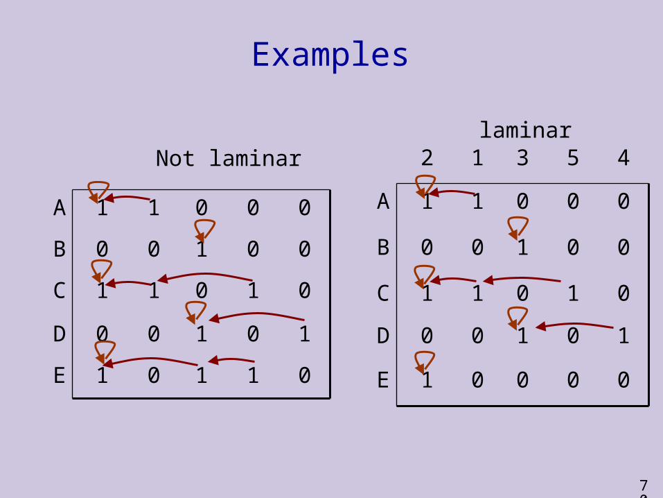
Examples
00001E
10100D
01011C
00100B
00011A
45312laminar
01101E
10100D
01011C
00100B
00011A
Not laminar
71
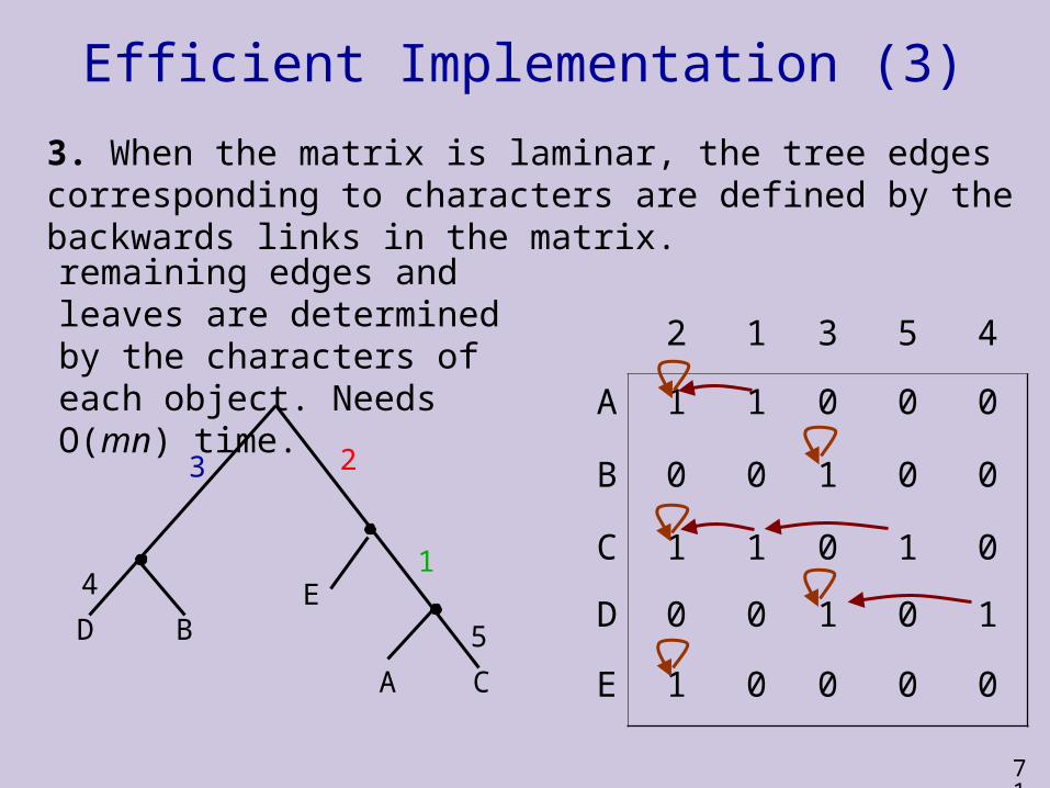
Efficient Implementation (3)
3. When the matrix is laminar, the tree edges corresponding to characters are defined by the backwards links in the matrix.
2 1 3 5 4
A 1 1 0 0 0
B 0 0 1 0 0
C 1 1 0 1 0
D 0 0 1 0 1
E 1 0 0 0 0A
ED
C
B
4
3 2
1
5
remaining edges and leaves are determined by the characters of each object. Needs O(mn) time.