Combinatorial Approaches to Haplotype Inference

Dan Gusfield

CS, UC Davis

Three topics

• Super-charging Clark’s method of 1990 - Two ideas: Min haps selection + Consensus

• Follow-on to Haplotyping By Perfect Phylogeny - a more biological view, and phase transitions, recombinations (?)

• Computing True Parsimony Solutions, Clark/Parsimony hybrids - Integer Programming

Topic I: Supercharging Clark’s Method

S. Orzack, D. Gusfield, V. Stanton

Genetics, in revision

Generic Clark Method

Given a known haplotype H (original homozygote or single-siteheterozygote, or previously inferred), and an unresolvedgenotype G, if G can be explained by H and another vector H’,then call H’ a known haplotype, available for additional inferrals.

example: H 0 1 0 0 1 G 2 1 0 2 2 G is “resolved” by H and H’ ------------------ H’ 1 1 0 1 0

Clark (1990) Randomize choices, and do the computations manytimes to find an execution (run) that explains the most genotypes.

In a single run, repeat the basic step until stuck - resolve as many genotypes as possible in the data.

Basic Step:

Many variations of Clark

• Variations based on which parts are randomized.• We closely examine eight variations on a real

data set. Variation 1 randomizes every decision - probably more than Clark originally intended.

• Truth in advertising - we implemented our own Clark versions - did not actually use Clark’s software.

Super-charging Clark’s method

Why? The reported accuracy is significantly

less than that of PHASE and HAPLOTYPER.

Answers: 1) Scale

2) Deeper insight

Supercharging Clark’s Method

• How? Run many times (10,000) to get (generally) a huge range of solutions, often 10,000 different solutions. This is a good thing!

• Select the (few - in the 10’s) runs that use the smallest number of distinct haplotypes over the 10,000 runs. Let S be that set of runs.

• Vote - for each individual find the haplotype pair used most often in S. This gives the Consensus solution.

Results on Lab Determined Data

• APOE locus

• 80 individuals, 9 polymorphic sites, 47 ambiguous after homozygotes and single-site heterozygotes identified - lab determined haplotypes

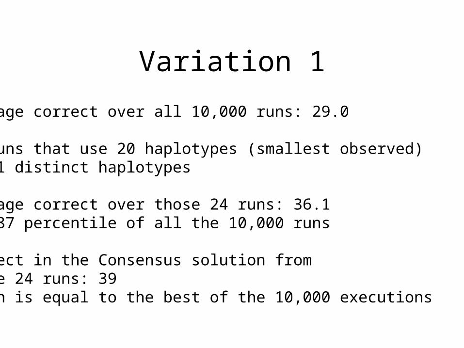
Variation 1

Average correct over all 10,000 runs: 29.0

24 runs that use 20 haplotypes (smallest observed)or 21 distinct haplotypes

Average correct over those 24 runs: 36.10.9987 percentile of all the 10,000 runs

Correct in the Consensus solution from those 24 runs: 39which is equal to the best of the 10,000 executions

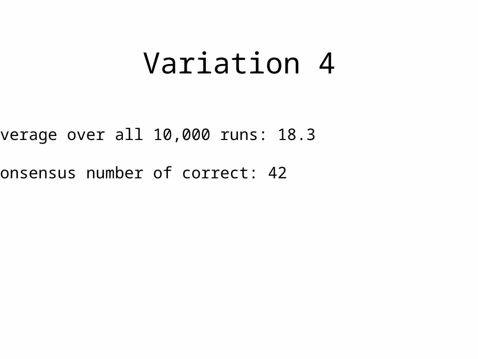
Variation 4

Average over all 10,000 runs: 18.3

Consensus number of correct: 42

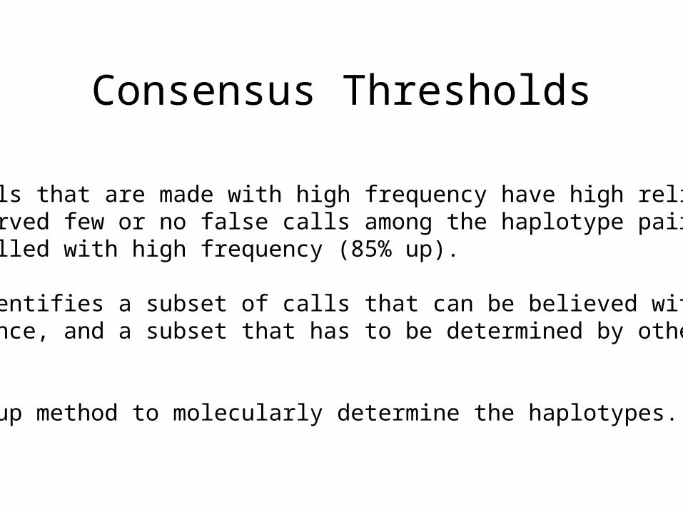
Consensus Thresholds

The calls that are made with high frequency have high reliability.We observed few or no false calls among the haplotype pairs that were called with high frequency (85% up).

This identifies a subset of calls that can be believed with highconfidence, and a subset that has to be determined by other means.

Bottom-up method to molecularly determine the haplotypes.

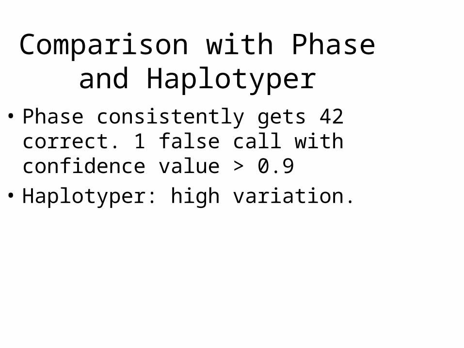
Comparison with Phase and Haplotyper

• Phase consistently gets 42 correct. 1 false call with confidence value > 0.9

• Haplotyper: high variation.

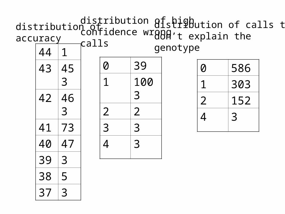
44 1

43 453

42 463

41 73

40 47

39 3

38 5

37 3

distribution ofaccuracy

0 39

1 1003

2 2

3 3

4 3

distribution of highconfidence wrong calls

0 586

1 303

2 152

4 3

distribution of calls thatdon’t explain the genotype

Topic 2: Haplotyping as Perfect Phylogeny

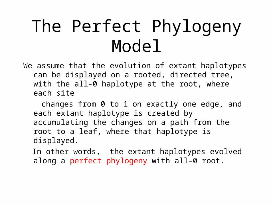
The Perfect Phylogeny Model

We assume that the evolution of extant haplotypes can be displayed on a rooted, directed tree, with the all-0 haplotype at the root, where each site

changes from 0 to 1 on exactly one edge, and each extant haplotype is created by accumulating the changes on a path from the root to a leaf, where that haplotype is displayed.

In other words, the extant haplotypes evolved along a perfect phylogeny with all-0 root.

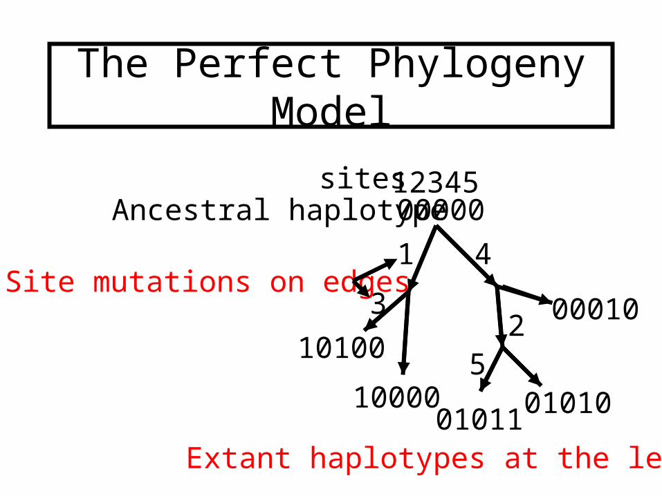
The Perfect Phylogeny Model

00000

1

2

4

3

510100

1000001011

00010

01010

12345sitesAncestral haplotype

Extant haplotypes at the leaves

Site mutations on edges

Justification for Perfect Phylogeny Model

• In the absence of recombination each haplotype of any individual has a single parent, so tracing back the history of the haplotypes in a population gives a tree.

• Recent strong evidence for long regions of DNA with no recombination. Key to the NIH haplotype mapping project. (See NYT October 30, 2002)

• Mutations are rare at selected sites, so are assumed non-recurrent.

• Connection with coalescent models.

Solving the Haplotype Phylogeny Problem (PPH) in nearly linear

time

• Finds if there is a solution.

• Counts the number of solutions.

• Implicitly represents all the solutions

Gusfield, RECOMB, April 2002

Program PPH

• Program PPH solves the perfect phylogeny haplotyping problem using the graph realization approach. It solves problems with 50 sites and 100 individuals in about 1 second.

• Program PPH can be obtained at

www.cs.ucdavis.edu/~gusfield

An alternative solution

Recently, we developed an algorithm that is not basedon graph realization, and which is much easier to understand.However, it runs in O(nm^2) time. V. Bafna, D. Gusfield, G. Lancia, S. Yooseph

See Gusfield’s website.

The implicit representation: A column partition

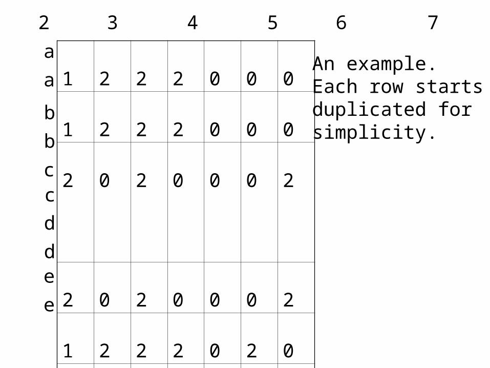
The algorithm partitions the sites (columns) into classes,such that within any class, the phase relationship (in, orout of phase)of any two columns is INVARIANT over all perfect phylogenies for the data.

Between any two classes, the phase relationship can beset ARBITRARILLY. All solutions can be genetatedin this way.

That is the representation of the set of all solutions. The number of solutions is always a power of two.

1 2 2 2 0 0 0

1 2 2 2 0 0 0

2

0 2 0 0 0 2

2 0 2 0 0 0 2

1 2 2 2 0 2 0

1 2 2 2 0 2 0

1 2 2 0 2 0 0

1 2 2 0 2 0 0

2 2 0 0 0 2 0

2 2 0 0 0 2 0

a

a

b

b

cc

d

ed

e

1 2 3 4 5 6 7

An example.Each row startsduplicated forsimplicity.

1 1 0 0 0 0 0

1 0 1 1 0 0 0

1

0 1 0 0 0 0

0 0 0 0 0 0 1

1 1 0 0 1 0 0

1 0 1 1 0 0 0

1 1 0 0 0 1 0

1 0 1 0 0 0 0

1 1 0 0 1 0 0

0 0 0 0 0 0 0

a

a

b

b

cc

d

ed

e

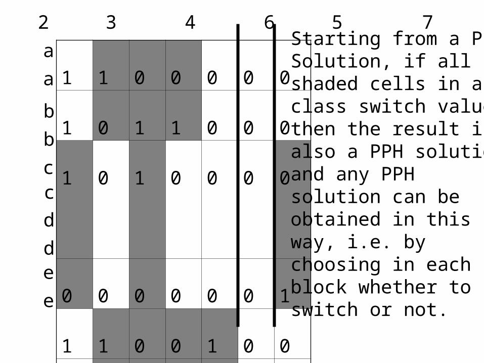
1 2 3 4 6 5 7Starting from a PPHSolution, if all shaded cells in aclass switch value,then the result isalso a PPH solution,and any PPHsolution can be obtained in this way, i.e. by choosing in eachblock whether toswitch or not.

Secondary information and optimization

• The partition shows explicitly what added information is useful and what is redundant. Information about the relationship of a pair of columns is redundant if and only if they are in the same class of the column partition. Apply this successively as additional information is obtained.

• Problem: Minimize the number of haplotype pairs (individuals) that need be laboratory determined in order to find the correct tree.

• Minimize the number of (individual, site1, site2) triples whose phase relationship needs to be determined, in order to find the correct tree.

The implicit representation of all solutions providesa framework for solving these secondary problems,as well as other problems involving the use ofadditional information, and specific tree-selectioncriteria.

A Phase-Transition

Problem, as the ratio of sites to genotypes changes,how does the probability that the PPH solution isunique change?

For greatest utility, we want genotype data where thePPH solution is unique.

Intuitively, as the ratio of genotypes to sites increases,the probability of uniqueness increases.

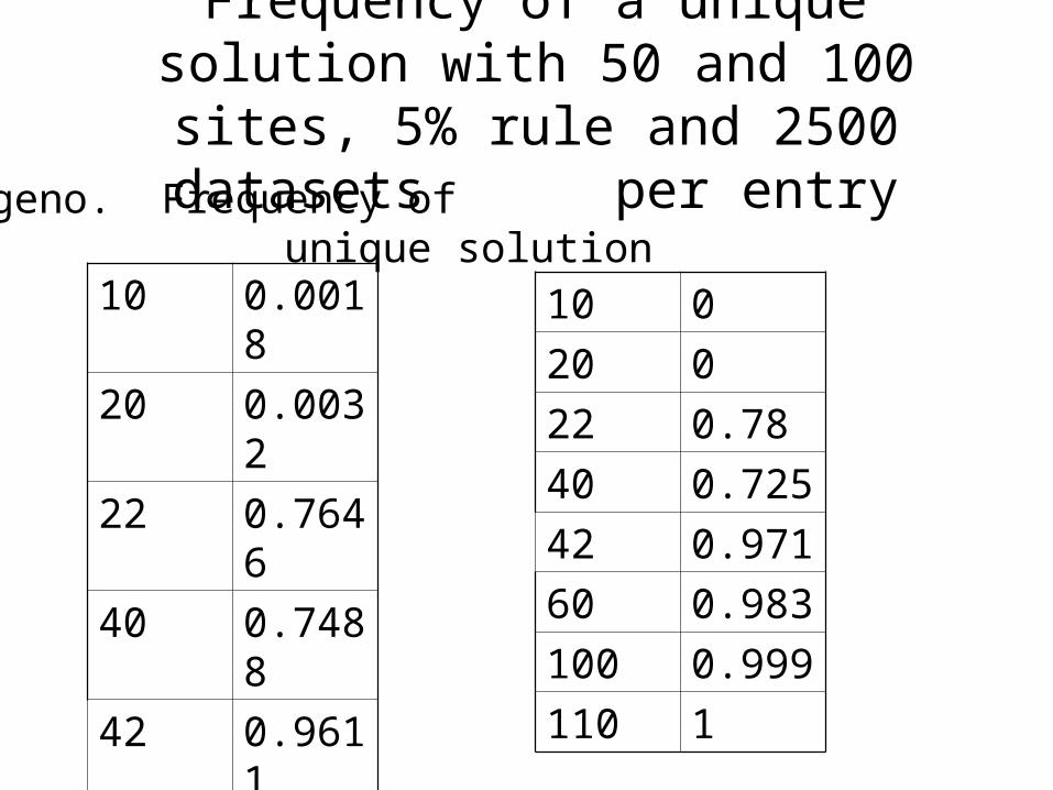
Frequency of a unique solution with 50 and 100 sites, 5% rule and 2500 datasets

per entry

10 0.0018

20 0.0032

22 0.7646

40 0.7488

42 0.9611

70 0.994

130 0.999

140 1

# geno. Frequency of unique solution

10 0

20 0

22 0.78

40 0.725

42 0.971

60 0.983

100 0.999

110 1

Data with recombination

If the genotype data does not fit a perfect phylogeny,we decompose the sites (greedily left to right) intomaximal intervals that do fit a unique perfect phylogeny.

Experimental results: number of intervals reduces toabout a tenth. The solutions are highly accurate in eachinterval. Then we have a phase problem again betweenthe intervals.The final haplotype determination can be made with one site per interval, greatly reducing any lab effort.

No Approximations - find the true smallest, and know forsure you have it !

Topic 3: The True Parsimony Objective

For a set of genotypes, find a Smallest set H of haplotypes, such that each genotype can be explained by a pair of haplotypes in H.

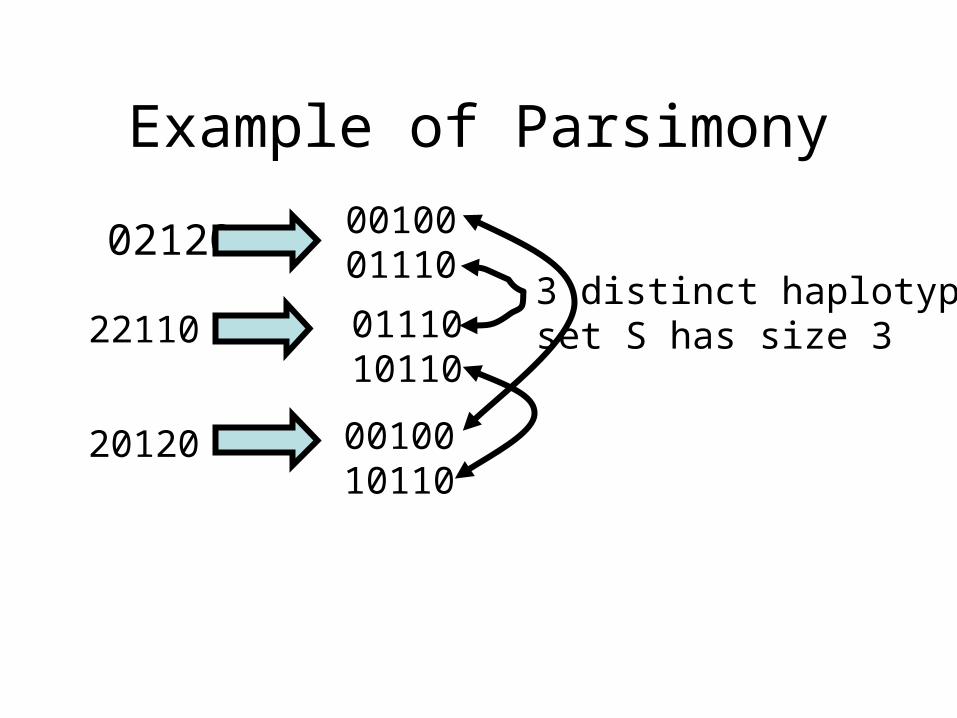
Example of Parsimony

02120 0010001110

22110 01110 10110

20120 0010010110

3 distinct haplotypesset S has size 3

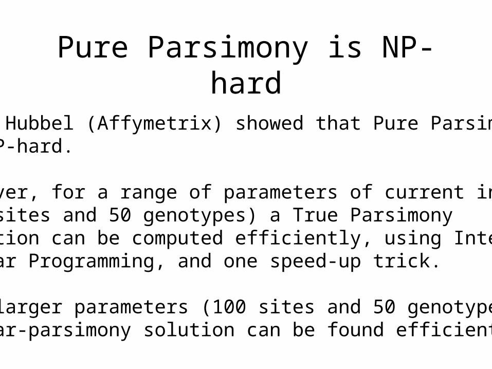
Pure Parsimony is NP-hard

Earl Hubbel (Affymetrix) showed that Pure Parsimonyis NP-hard.

However, for a range of parameters of current interest(50 sites and 50 genotypes) a True Parsimony solution can be computed efficiently, using IntegerLinear Programming, and one speed-up trick.

For larger parameters (100 sites and 50 genotypes)A near-parsimony solution can be found efficiently.

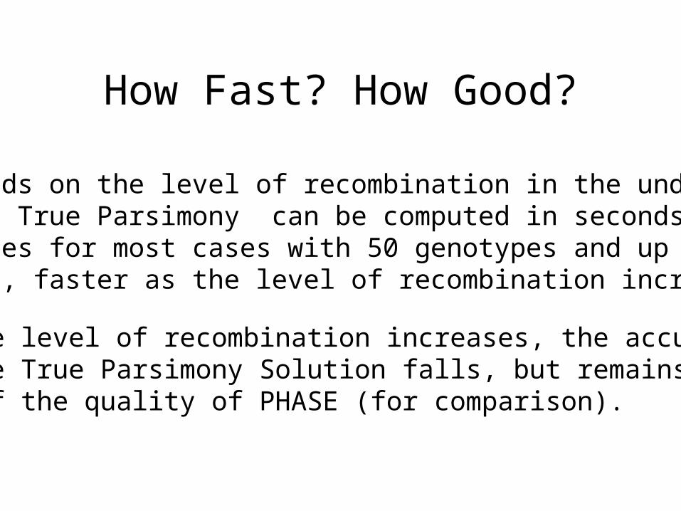
How Fast? How Good?

Depends on the level of recombination in the underlyingdata. True Parsimony can be computed in seconds tominutes for most cases with 50 genotypes and up to 60sites, faster as the level of recombination increases.

As the level of recombination increases, the accuracyof the True Parsimony Solution falls, but remains within10% of the quality of PHASE (for comparison).

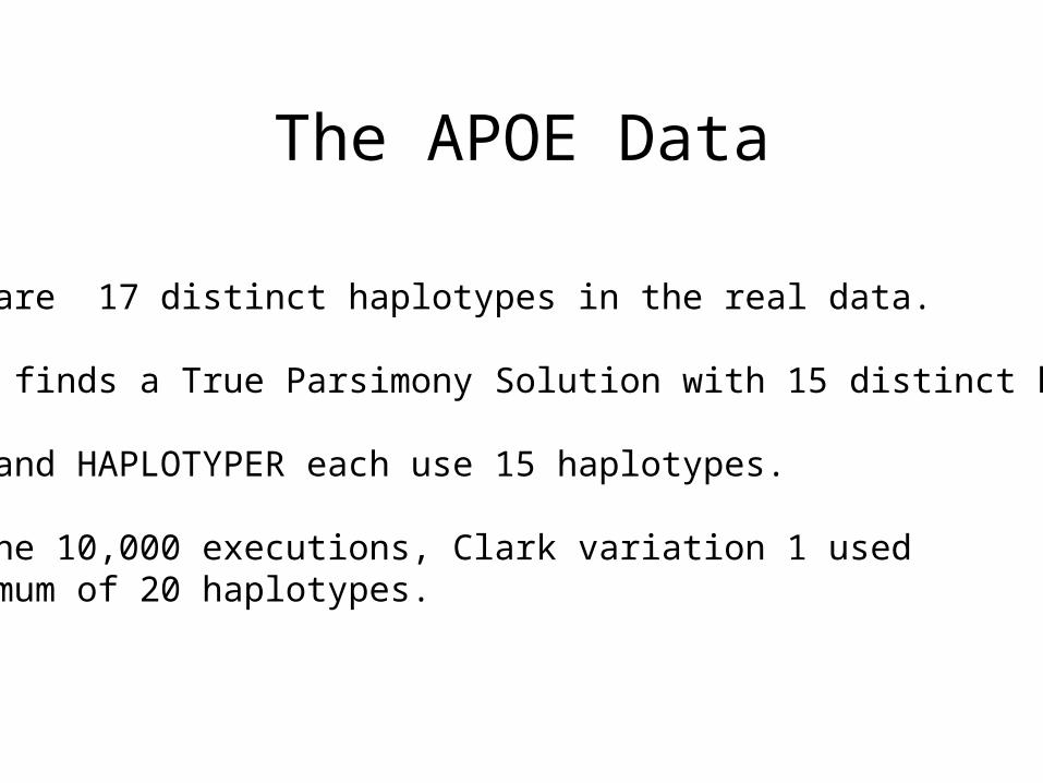
The APOE Data

There are 17 distinct haplotypes in the real data.

The IP finds a True Parsimony Solution with 15 distinct haplotypes.

PHASE and HAPLOTYPER each use 15 haplotypes.

Over the 10,000 executions, Clark variation 1 useda minimum of 20 haplotypes.

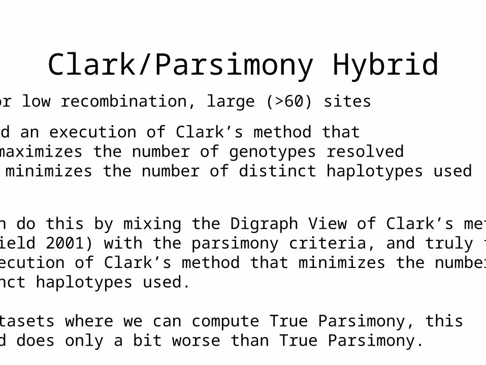
Clark/Parsimony Hybrid

Find an execution of Clark’s method that a) maximizes the number of genotypes resolvedb) minimizes the number of distinct haplotypes used

We can do this by mixing the Digraph View of Clark’s method (Gusfield 2001) with the parsimony criteria, and truly findan execution of Clark’s method that minimizes the number ofdistinct haplotypes used.

On datasets where we can compute True Parsimony, thishybrid does only a bit worse than True Parsimony.

For low recombination, large (>60) sites

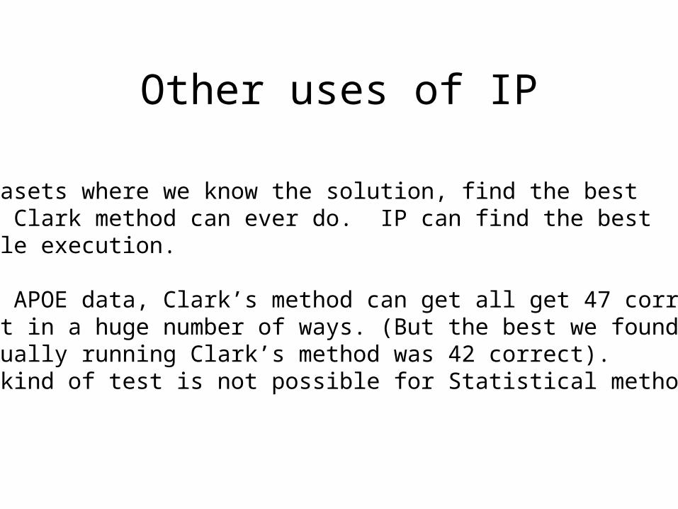
Other uses of IP

On datasets where we know the solution, find the bestthat a Clark method can ever do. IP can find the bestpossible execution.

On the APOE data, Clark’s method can get all get 47 correct! In fact in a huge number of ways. (But the best we foundby actually running Clark’s method was 42 correct). This kind of test is not possible for Statistical methods.

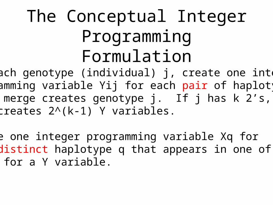
The Conceptual Integer Programming Formulation

For each genotype (individual) j, create one integerprogramming variable Yij for each pair of haplotypeswhose merge creates genotype j. If j has k 2’s, thenThis creates 2^(k-1) Y variables.

Create one integer programming variable Xq forEach distinct haplotype q that appears in one of thepairs for a Y variable.

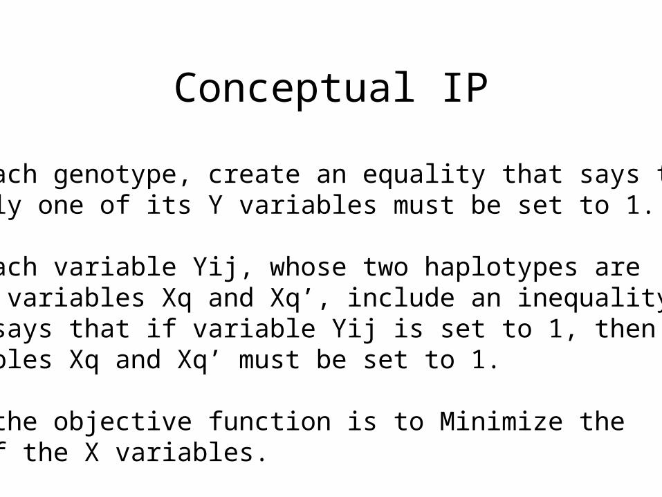
Conceptual IP

For each genotype, create an equality that says thatexactly one of its Y variables must be set to 1.

For each variable Yij, whose two haplotypes aregiven variables Xq and Xq’, include an inequalitythat says that if variable Yij is set to 1, then bothvariables Xq and Xq’ must be set to 1.

Then the objective function is to Minimize thesum of the X variables.

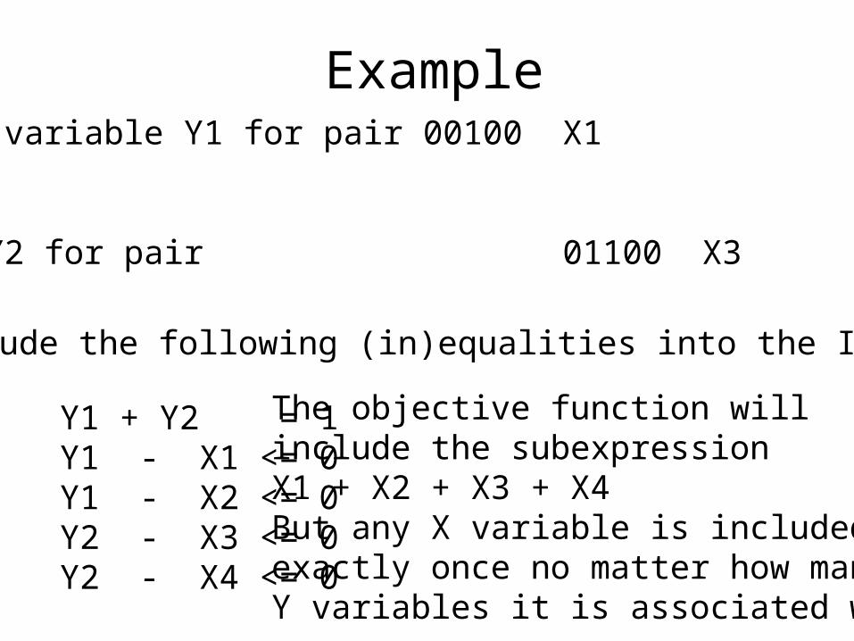
Example02120 Creates a Y variable Y1 for pair 00100 X1 01110 X2

and a Y variable Y2 for pair 01100 X3 00110 X4

Y1 + Y2 = 1Y1 - X1 <= 0Y1 - X2 <= 0Y2 - X3 <= 0Y2 - X4 <= 0

Include the following (in)equalities into the IP

The objective function willinclude the subexpressionX1 + X2 + X3 + X4But any X variable is includedexactly once no matter how manyY variables it is associated with.

Efficiency Tricks

Ignore any Y variable and its two X variables if those Xvariables are associated with no other Y variable. TheResulting IP is much smaller, and can be used to findthe optimal to the conceptual IP.

Also, we need not enumerate all X pairs for a given genotype, but can efficiently recognize the pairs weneed.

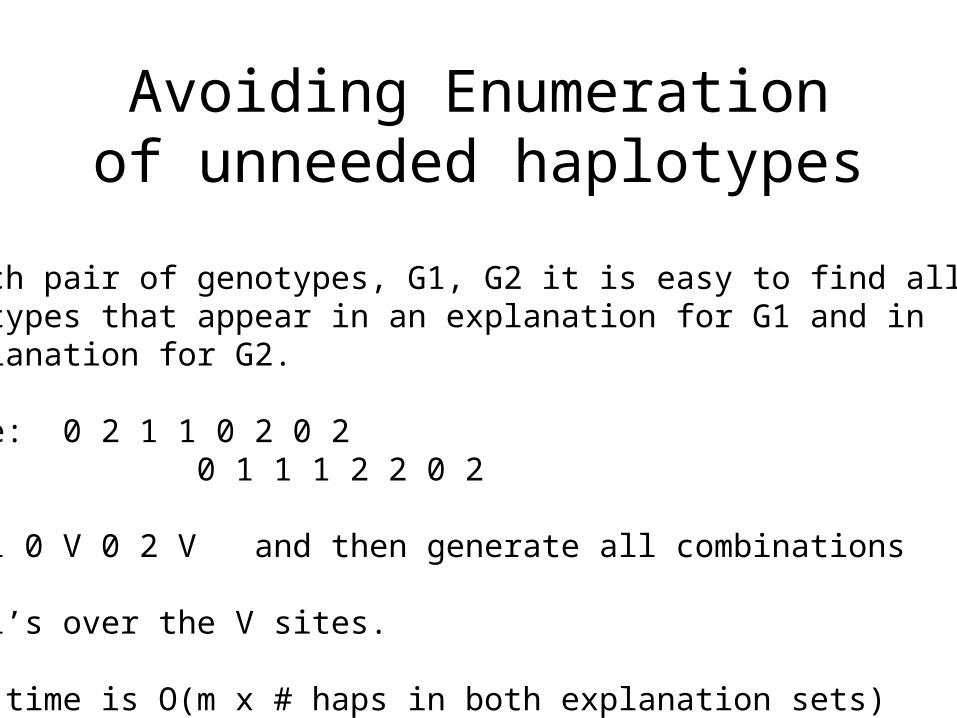
Avoiding Enumeration of unneeded haplotypes

For each pair of genotypes, G1, G2 it is easy to find all the haplotypes that appear in an explanation for G1 and inan explanation for G2.

Example: 0 2 1 1 0 2 0 2 0 1 1 1 2 2 0 2

0 1 1 1 0 V 0 2 V and then generate all combinations

of 0,1’s over the V sites.

So the time is O(m x # haps in both explanation sets)

Recombination Helps!

As the level of recombination increases, the number ofhaps in two explanation sets decreases, so the size ofthe IP falls.

Full paper on Parsimony

See the technical report: Haplotyping by Pure Parsimonyavailable atwwwcsif.cs.ucdavis.edu/~gusfield/

Thanks to Andy, Sorin and Mike.