€¦ · technische universit¨at m¨unchen max-planck-institut f¨ur extraterrestrische physik...
TRANSCRIPT

First Light for the Next Generationof Compton and Pair Telescopes
Andreas Christian Zoglauer


Technische Universitat Munchen
Max-Planck-Institut fur extraterrestrische PhysikGarching bei Munchen
First Light for the Next Generationof Compton and Pair Telescopes
Andreas Christian Zoglauer
Vollstandiger Abdruck der von der Fakultat fur Physik der Technischen Universitat Munchenzur Erlangung des akademischen Grades eines
Doktors der Naturwissenschaften
genehmigten Dissertation.
Vorsitzender: Univ.-Prof. Dr. Andrzej Jerzy BurasPrufer der Dissertation: 1. apl. Prof. Dr. Volker Schonfelder
2. Univ.-Prof. Dr. Franz von Feilitzsch
Die Dissertation wurde am 17.11.2005 bei der Technischen Universitat Munchen eingereicht unddurch die Fakultat fur Physik am 8.12.2005 angenommen.

Zusammenfassung
Gamma-Astronomie im MeV-Bereich von einigen hundert keV bis zu einigen zehn MeV lieferteinzigartige Informationen uber das Universum: Die verhaltnismaßig geringe Wechselwirkungs-wahrscheinlichkeit von Gammastrahlen ermoglicht es Quellen zu studieren, deren Strahlung beiniedrigeren Energien vom umgebenden Material stark absorbiert wird. Linien aus Kernzerfallenliefern Informationen uber Ursprung und Verteilung einzelner Isotope im Kosmos. Ein Instru-ment, das effizient sowohl Compton- als auch Paarereignisse — die beiden dominanten Wech-selwirkungsprozesse — aufzeichnet, konnte bedeutend empfindlichere Beobachtungen in diesemEnergiebereich ermoglichen.
Die Entwicklung einer moglichen zukunftigen Mission fur “Medium Energy Gamma-rayAstronomy” wurde am Max-Planck-Institut fur extraterrestrische Physik in Garching unter demNamen MEGA vorangetrieben. MEGA besteht aus einem Spurdetektor und einem Kalorimeterund soll mindestens den Energiebereich von 0,4 MeV bis 50 MeV abdecken. Der Spurdetektorbesteht aus einem Stapel doppelseitiger Silizium-Streifendetektoren, in denen die Compton-Streuung oder Paarerzeugung stattfindet. Er misst die Richtung und die Energie der Elektronenund Positronen. Ein Kalorimeter aus CsI(Tl) Kristallen umgibt den Spurdetektor. Es soll alleSekundarteilchen komplett absorbieren und aufzeichnen.
Die Kenntnis der Streurichtung der Compton Elektronen ermoglicht es, den Ursprung ei-nes Ereignisses auf ein kleines Segment des klassischen Kegels aller moglichen Einfallsrichtun-gen einzuschranken. Um diese Information auszunutzen, mußten vollig neue Methoden fur diekomplette Datenanalysekette entwickelt werden — von Messungen oder Simulationen uber dieEreignisrekonstruktion bis hin zur Bildrekonstruktion.
Die Datenanalyse fur ein kombiniertes Compton- und Paarteleskop beinhaltet zwei großeHerausforderungen. Eine davon ist die korrekte Rekonstruktion jedes einfallenden Photons ausden gemessenen Energie- und Positionsinformationen. Ein realer Detektor hat immer Fehler undEigenheiten, die zu suboptimalen Meßdaten fuhren. Um die von einem realen Detektor gemesse-nen Ereignisse erfolgreich rekonstruieren zu konnen, ist ein detailliertes Verstandnis der Wech-selwirkungsprozesse im Instrument eine Grundvoraussetzung. Ausgehend von idealen Compton-und Paar-Wechselwirkungen werden die Auswirkung von Moliere-Streuung auf die gemessenenElektronenspuren diskutiert, sowie die Folgen von fehlenden oder ungenugenden Energie- oderRichtungsmessungen als auch von Dopplerverbreiterung erlautert. Insbesondere im Falle derkomplexen Rekonstruktion von Compton-Ereignisreihenfolgen fuhrt eine detaillierte Beschrei-bung eines an die Wechselwirkungsphysik angepassten, mehrdimensionalen Ereignisdatenraumszu optimierten Ereignisauswahl-Kriterien und einer Diskussion ihrer Anwendbarkeit auf ver-schiedene Ereignistypen. Es wurden zwei fundamental unterschiedliche Methoden fur die Ereig-nisrekonstruktion entwickelt: Die eine basiert auf Korrelationen zur Rekonstruktion der Elektro-nenspur und einem χ2-Ansatz zur Bestimmung der korrekten Compton-Sequenz, die andere aufBayes-Statistik und einer mehrdimensionalen Detektor-Antwortfunktion. Die Leistungsfahigkeitbeider Algorithmen wird diskutiert. Simulationen eines MEGA-Satelliteninstruments zeigen, daßder Bayes-Ansatz im Mittel zu einer um einen Faktor 1,5 besseren Sensitivitat fuhrt.
Die zweite Herausforderung ist die Rekonstruktion von Bildern aus den Ereignissen. Ein Algo-rithmus basierend auf der List-Mode Maximum-Likelihood Expectation-Maximization Methodewurde fur die MEGA-Bildanalyse weiterentwickelt. Dieser Ansatz ermoglicht es problemlos dieverschiedenen Ereignistypen (Compton-Ereignisse mit und ohne Elektronenspur sowie Paarer-eignisse) in ein Bild zusammenzufassen. Die hierfur entwickelten Abbildungs-Antwortfunktionenberucksichtigen die meisten Aspekte des Verhaltens dieses komplexen Detektors.
Der MEGA Prototyp, der grob ein Zwolftel des Volumens eines denkbaren Satelliteninstru-ments besitzt, wurde sowohl mit radioaktiven Laborquellen als auch an der High Intensity Gam-ma Source an der Duke University kalibriert. Messungen mit monoenergetischen, 100% linear
i

polarisierten Photonen im Energiebereich von 710 keV bis 49 MeV (ΔE/E< 2%) ermoglichendie Bestimmung der Spektral-, Abbildungs- und Polarisationseigenschaften des Prototypen.
Im MEGA Prototypen werden Gammaquanten, vor allem mit hoheren Energien, oft nichtvollstandig absorbiert. Grunde fur eine unvollstandige Erfassung der gesamten Wechselwirkungs-kette sind Verluste in passiven Strukturmaterialien, Instabilitaten der Elektronik sowie die un-vollstandige Abdeckung der unteren Halfte des Spurdetektors. Außerdem fuhren die moderateEnergieauflosung vor allem des Kalorimeters und die vorgenannten Instabilitaten gemeinsam zueiner signifikanten Verbreiterung des Photopeaks. Deshalb ergeben die Beschleunigermessungenmit dem Prototypen einzig bei 710 keV einen Photopeak (41 keV 1σ-Breite).
Trotz der sehr moderaten Energieauflosung konnte die Winkelauflosung des Prototypen be-stimmt werden. Fur Comptonereignisse ohne Elektronenspur wird die Winkelauflosung von ∼7◦
bei 710 keV zu ∼4◦ bei 2 MeV stetig besser. Gleiches gilt fur Comptonereignisse mit Elektronen-spur (∼9◦ bei 2 MeV, ∼3◦ bei 8 MeV) und Paarereignisse (12◦ bei 12 MeV, 4,5◦ bei 49 MeV).Punktquellen von 710 keV bis 49 MeV mit Einfallswinkeln zwischen 0◦ und 80◦ werden pro-blemlos auf die korrekte Position rekonstruiert — selbst wenn nur ∼100 komplett absorbierteEreignisse gemessen wurden. Außerdem konnte gezeigt werden, dass der Prototyp — zusam-men mit den Ereignisrekonstruktions- und Bildrekonstruktionsalgorithmen — mehrere Quellendifferenzieren und ausgedehnte Quellen korrekt abbilden kann.
Da die azimuthale Compton-Streurichtung gemaß dem differentiellen Klein-Nishina Wir-kungsquerschnitt von der Polarisation des einfallenden Photons abhangt, ist jedes Comptontele-skop automatisch auch ein Polarimeter. Bei 710 keV, wo die gemessene Polarisationsmodulationwesentlich von den Detektoreigenschaften beeinflußt wird, konnte eine Modulation von 17% mitdem MEGA-Prototypen nachgewiesen werden. Wie erwartet fallt fur 100% polarisierte Strah-lung mit steigender Photonenenergie die Modulation auf 13% bei 2 MeV und auf 6% bei 5MeV.
Die Eigenschaften eines moglichen Satelliteninstruments (hier basierend auf der Pre-Phase AStudie fur MEGA) wurden auf der Basis ausfuhrlicher Simulationen vorhergesagt. Diese umfas-sen Simulationen von Kontinuums- und Linienquellen sowie von allen Hintergrundkomponenten,die in einer aquatorialen Umlaufbahn in 525 km Hohe erwartet werden. Fur das Satelliteninstru-ment aus der pre-Phase A Studie ist eine Winkelauflosung von ∼4◦ bei 511 keV fur Comptoner-eignisse ohne Spur und ∼3◦ bei 1809 keV fur Comptonereignisse mit Spur zu erwarten; beide kon-vergieren fur hohere Energien gegen die durch die Detektor-Positionsauflosung gegebene Grenzevon ∼1◦. Die gesamte effektive Flache im Photopeak fur alle Compton-Ereignisse ohne weitereEreignisauswahl betragt ∼120 cm2 bei 511 keV, ∼50 cm2 bei 1809 keV und ∼2 cm2 bei 6130 keV.Fur Paarereignisse betragt die effektive Flache vor jeglicher Ereignisauswahl ∼35 cm2 bei 10 MeVund ∼60 cm2 bei 50 MeV. Nach Anwendung optimierter Ereignisauswahlkriterien wird nachfunf Jahren Himmelsdurchmusterung eine Kontinuumssensitivitat von ∼1 ·10−5 MeV/cm2/s um1MeV und ∼5 · 10−5 MeV/cm2/s um 50 MeV erzielt. Nach derselben Missionsdauer wird eineLiniensensitivitat von ∼4.3 · 10−6 γ/cm2/s bei 511 keV und ∼1.7 · 10−6 γ/cm2/s bei 1809 keVfur jeden beliebigen Punkt am Himmel erreicht. Fur eine Crab-ahnliche Quelle kann nach funfJahren Himmelsdurchmusterung eine lineare Polarisation von 0.5% nachgewiesen werden.
Einige Modifikationen des Satelliten-Instrumentkonzepts der pre-Phase A Studie, wie z.B.mehr Silizium im Spurdetektor oder eine Verbesserung der Energieauflosung der Kalorimeteruber die bereits angenommene hinaus, konnten dieses kombinierte Compton- und Paarteleskopweiter verbessern. MEGA konnte unerreicht sensitive Messungen im Kontinuum und in einzelnenLinien liefern und uberdies als erstes sensitives Compton-Polarimeter Neuland beschreiten undso die MeV-Gammaastronomie einen großen Schritt voranbringen.
ii

Abstract
Gamma-ray astronomy in the MeV regime, from a few hundred keV to several tens of MeV,can provide unique information about the universe: The high penetration power of the gammarays enables studies of highly obscured sources, and nuclear lines carry information about originand distribution of individual isotopes in the cosmos. A leap in observational capabilities inthis energy regime could be achieved by an instrument able to efficiently record events resultingfrom both dominating interaction mechanisms, Compton scattering and pair creation.
One potential future mission for Medium Energy Gamma-ray Astronomy is MEGA, whichhas been pursued at the Max-Planck-Institut fur extraterrestrische Physik in Garching. MEGAis intended to operate from 0.4 to at least 50 MeV and consists of a tracker and a calorimeter.The tracker is a stack of double-sided Silicon-strip detectors in which the Compton scattering orpair creation takes place. It measures the direction and energy of the electrons and positrons.A calorimeter consisting of CsI(Tl) crystals surrounds the tracker. It is intended to fully absorband measure all secondary particles.
The knowledge of the direction of the Compton recoil electron enables the reconstructionof the individual events not only to a Compton cone, but to a small segment of this cone. Asconsequence, a new set of data analysis tools had to be developed, covering the complete chainfrom measurements or simulations via event reconstruction to high-level data analysis such asimage reconstruction.
One of two major challenges of analyzing data from a combined Compton and pair telescopeis the reconstruction of the parameters of each original photon from the measured data, whichconsist only of several energy and position measurements. In order to properly reconstructevents recorded by a real-life detector, which always has some flaws resulting in less-than-perfect measurement data, the interaction processes in the instrument must be extremely wellunderstood. Along with picture-perfect Compton and pair interactions, the effects of Molierescattering on electron tracks are discussed as well as the effects of incomplete energy or directionmeasurements and Doppler broadening on Compton event reconstruction. For the complex taskof Compton sequence reconstruction in particular, the detailed description of a dedicated multi-dimensional event data space naturally leads to a discussion of possible event quality selectioncriteria and their applicability to different event types. Two independent event reconstructionalgorithms have been developed, one based on correlations for tracking the path of the electronand on a χ2 approach for reconstructing the sequence of Compton interactions, the other basedon Bayesian statistics and multi-dimensional detector response functions. The performance ofboth is evaluated. Simulations of a MEGA satellite instrument show that the Bayesian approachachieves on average a factor of 1.5 better overall sensitivity.
The second challenge is the reconstruction of sky images from the event data. A list-modemaximum-likelihood expectation-maximization approach has been chosen, and an enhanced al-gorithm has been developed for imaging with MEGA. This approach naturally allows to incor-porate all different event types (not tracked and tracked Compton events as well as pair events)into one image. Detailed imaging response descriptions have been developed which cover mostaspects of the complex behavior of the detector.
The MEGA prototype, which encompasses one twelfth of the volume of the satellite versionunder study, has been calibrated with laboratory radioactive sources and at the High IntensityGamma Source of the Free Electron Laser facility at Duke University. Exposures to monoener-getic (range 710 keV to 49 MeV, ΔE/E < 2%), 100% linearly polarized pencil beams allow thederivation of the spectral, imaging and polarization properties of this prototype instrument.
Especially high-energy gamma rays are not always completely absorbed in the MEGA pro-totype. Reasons for the incomplete measurement are the large amount of passive materials,electronics instabilities, and significant gaps in the prototype calorimeter. Moreover, the mod-
iii

est energy resolution primarily of the calorimeter modules and instabilities in the detector systemlead to a significantly broadened photo peak. As a result, the prototype beam measurementsdid not yield a significant photo peak except at 710 keV, where an energy resolution of ∼41 keV(1σ) was achieved.
Despite the modest spectral resolution, meaningful information about the angular resolutioncan be retrieved. For not tracked events, the angular resolution improves from ∼7◦ at 710 keV to∼4◦ at 2MeV, for tracked events from ∼9◦ at 2MeV to ∼3◦ at 8 MeV and for pair events from12◦ at 12 MeV to 4.5◦ at 49 MeV. Point sources from 710 keV up to 49 MeV as well as from 0◦
to 80◦ incidence can be easily reconstructed at the correct positions with the developed imagingalgorithms from every one of the Duke measurements — even if only ∼100 fully absorbed eventswere recorded. In addition, it could be shown that the prototype — in conjunction with theevent reconstruction and imaging algorithms — can correctly disentangle multiple sources andfaithfully image extended sources.
Since the azimuthal direction of Compton scattering according to the differential Klein-Nishina cross-section depends on the incident photon’s polarization, any Compton telescope isintrinsically sensitive to polarization. At 710 keV, where the retrieved polarization modulationis most influenced by detector limitations, a polarization modulation of 17% could be detectedwith the MEGA prototype. The expected modulation for 100% linearly polarized gamma raysdecreases with higher photon energy; modulations of 13% at 2 MeV and 6% at 5 MeV wereobtained.
The expected performance of one possible satellite instrument, based on the MEGA pre-phaseA study, has been derived from extensive simulations of continuum and gamma-ray line pointsources as well as all background components expected for an equatorial low-earth (525 km)orbit. This simulation approach is validated by the good agreement achieved between theMEGA prototype calibration measurements and corresponding Geant simulations. The satelliteinstrument of the pre-Phase A study is expected to achieve an angular resolution of ∼4◦ for nottracked events at 511 keV and ∼3◦ for tracked events at 1809 keV, both converging towards thedetector position resolution limit at ∼1◦ for higher energies. The total photo-peak effective areafor all Compton events before background cuts is ∼120 cm2 at 511 keV, ∼50 cm2 at 1809 keV, and∼2 cm2 at 6130 keV. For pair events without any event restrictions the effective area is ∼35 cm2
at 10 MeV and ∼60 cm2 at 50 MeV. Applying optimized event selections results in an averagecontinuum sensitivity after 5 years all-sky survey of ∼1 · 10−5 MeV/cm2/s at around 1MeV and∼5 · 10−5 MeV/cm2/s at around 50 MeV. In the same 5-year period, a narrow line sensitivity of∼4.3 · 10−6 γ/cm2/s at 511 keV and ∼1.7 · 10−6 γ/cm2/s at 1809 keV would be achieved for anyarbitrary point on the sky. For a Crab-like source, a 0.5% linear polarization can be detectedafter 5 years all-sky survey.
Some changes to the pre-Phase A satellite instrument design, such as simply increasingthe total amount of Silicon or finding a way to further improve the energy resolution in thecalorimeters, could improve the performance of this tracking Compton and pair telescope evenfurther, enabling MEGA to provide a significant leap in continuum and narrow-line sensitivityas well as polarimetry for medium-energy gamma-ray astronomy.
iv
Contents
Zusammenfassung i
Abstract iii
Table of contents v
I Measuring extraterrestrial gamma rays 1
1 New mission in Medium-Energy Gamma-ray Astronomy 31.1 Medium-Energy Gamma-ray Astronomy . . . . . . . . . . . . . . . . . . . . . . . 4
1.1.1 Cosmic accelerators . . . . . . . . . . . . . . . . . . . . . . . . . . . . . . 41.1.2 Nucleosynthesis . . . . . . . . . . . . . . . . . . . . . . . . . . . . . . . . . 41.1.3 Capture, annihilation and deexcitation . . . . . . . . . . . . . . . . . . . . 61.1.4 Other sources of interest . . . . . . . . . . . . . . . . . . . . . . . . . . . . 7
1.2 Instrumentation for medium-energy gamma-ray astronomy . . . . . . . . . . . . . 71.2.1 Spatial and temporal modulation . . . . . . . . . . . . . . . . . . . . . . . 81.2.2 Single event detector systems . . . . . . . . . . . . . . . . . . . . . . . . . 91.2.3 Focusing gamma-rays . . . . . . . . . . . . . . . . . . . . . . . . . . . . . 11
1.3 MEGA - A telescope for medium-energy gamma-ray astronomy . . . . . . . . . . 12
2 Interaction processes 152.1 Interactions of electrons with matter . . . . . . . . . . . . . . . . . . . . . . . . . 15
2.1.1 Moliere scattering of electrons . . . . . . . . . . . . . . . . . . . . . . . . . 152.1.2 Energy loss of electrons in matter . . . . . . . . . . . . . . . . . . . . . . 17
2.2 Compton scattering . . . . . . . . . . . . . . . . . . . . . . . . . . . . . . . . . . 182.2.1 Kinematics . . . . . . . . . . . . . . . . . . . . . . . . . . . . . . . . . . . 192.2.2 Cross-sections . . . . . . . . . . . . . . . . . . . . . . . . . . . . . . . . . 202.2.3 Polarization . . . . . . . . . . . . . . . . . . . . . . . . . . . . . . . . . . 202.2.4 Incomplete measurement . . . . . . . . . . . . . . . . . . . . . . . . . . . 222.2.5 Angular resolution determination . . . . . . . . . . . . . . . . . . . . . . 252.2.6 Doppler broadening as a lower limit to the angular resolution of a Compton
telescope . . . . . . . . . . . . . . . . . . . . . . . . . . . . . . . . . . . . 272.3 Pair production . . . . . . . . . . . . . . . . . . . . . . . . . . . . . . . . . . . . 30
II New analysis techniques for combined Compton and pair telescopes 33
3 Simulation and data analysis overview 353.1 From detector measurements to hits . . . . . . . . . . . . . . . . . . . . . . . . . 353.2 From simulations to hits . . . . . . . . . . . . . . . . . . . . . . . . . . . . . . . . 36
v
3.3 Event reconstruction and response generation . . . . . . . . . . . . . . . . . . . . 373.4 High level data analysis . . . . . . . . . . . . . . . . . . . . . . . . . . . . . . . . 383.5 The scope of MEGAlib . . . . . . . . . . . . . . . . . . . . . . . . . . . . . . . . . 38
4 Event reconstruction 414.1 The basic idea . . . . . . . . . . . . . . . . . . . . . . . . . . . . . . . . . . . . . 41
4.1.1 Tasks and problems . . . . . . . . . . . . . . . . . . . . . . . . . . . . . . 414.1.2 Outline of the event reconstruction . . . . . . . . . . . . . . . . . . . . . 434.1.3 Approaches for complex reconstruction tasks . . . . . . . . . . . . . . . . 44
4.2 Clusterizing . . . . . . . . . . . . . . . . . . . . . . . . . . . . . . . . . . . . . . . 454.3 Identifying and reconstructing pair events . . . . . . . . . . . . . . . . . . . . . . 46
4.3.1 Method . . . . . . . . . . . . . . . . . . . . . . . . . . . . . . . . . . . . . 474.3.2 Performance . . . . . . . . . . . . . . . . . . . . . . . . . . . . . . . . . . 49
4.4 Compton electron tracking . . . . . . . . . . . . . . . . . . . . . . . . . . . . . . 514.4.1 The data space of electron tracking . . . . . . . . . . . . . . . . . . . . . 514.4.2 Identification of Compton electron tracks . . . . . . . . . . . . . . . . . . 53
4.5 Compton sequence reconstruction . . . . . . . . . . . . . . . . . . . . . . . . . . 604.5.1 Characteristics of the data space . . . . . . . . . . . . . . . . . . . . . . . 614.5.2 Classic Compton sequence reconstruction . . . . . . . . . . . . . . . . . . 704.5.3 Bayesian Compton sequence reconstruction . . . . . . . . . . . . . . . . . 72
4.6 Combined Compton reconstruction performance . . . . . . . . . . . . . . . . . . 75
5 Image reconstruction 795.1 Selecting an algorithm . . . . . . . . . . . . . . . . . . . . . . . . . . . . . . . . . 795.2 The list-mode algorithm . . . . . . . . . . . . . . . . . . . . . . . . . . . . . . . . 805.3 Imaging response of a Compton and pair telescope . . . . . . . . . . . . . . . . . 83
III The MEGA prototype and its performance 87
6 The MEGA Prototype 896.1 Setup of the prototype instrument . . . . . . . . . . . . . . . . . . . . . . . . . . 89
6.1.1 Tracker . . . . . . . . . . . . . . . . . . . . . . . . . . . . . . . . . . . . . 906.1.2 Calorimeter . . . . . . . . . . . . . . . . . . . . . . . . . . . . . . . . . . . 916.1.3 Anti-coincidence shield . . . . . . . . . . . . . . . . . . . . . . . . . . . . . 926.1.4 Setup of the prototype . . . . . . . . . . . . . . . . . . . . . . . . . . . . . 92
6.2 Calibration measurements . . . . . . . . . . . . . . . . . . . . . . . . . . . . . . 93
7 Events and spectra 977.1 Event statistics . . . . . . . . . . . . . . . . . . . . . . . . . . . . . . . . . . . . . 977.2 Spectral response . . . . . . . . . . . . . . . . . . . . . . . . . . . . . . . . . . . 100
8 Imaging properties of the MEGA prototype 1078.1 Angular resolution . . . . . . . . . . . . . . . . . . . . . . . . . . . . . . . . . . . 107
8.1.1 The Compton regime . . . . . . . . . . . . . . . . . . . . . . . . . . . . . 1078.1.2 The pair regime . . . . . . . . . . . . . . . . . . . . . . . . . . . . . . . . 114
8.2 List-Mode Likelihood imaging of the prototype data . . . . . . . . . . . . . . . . 1168.2.1 Multiple sources . . . . . . . . . . . . . . . . . . . . . . . . . . . . . . . . 1168.2.2 Extended sources . . . . . . . . . . . . . . . . . . . . . . . . . . . . . . . . 1178.2.3 On axis imaging as a function of energy . . . . . . . . . . . . . . . . . . . 1198.2.4 Field of view . . . . . . . . . . . . . . . . . . . . . . . . . . . . . . . . . . 119
vi
9 The MEGA prototype as Compton polarimeter 1239.1 Data correction . . . . . . . . . . . . . . . . . . . . . . . . . . . . . . . . . . . . . 1239.2 Polarization response of the prototype . . . . . . . . . . . . . . . . . . . . . . . . 124
IV Steps towards a MEGA space mission 127
10 Expected performance of a MEGA satellite mission 12910.1 Necessary design improvements towards a satellite mission . . . . . . . . . . . . . 12910.2 A potential MEGA satellite . . . . . . . . . . . . . . . . . . . . . . . . . . . . . . 131
10.2.1 Simulation and orbital background . . . . . . . . . . . . . . . . . . . . . 13210.2.2 Event selections . . . . . . . . . . . . . . . . . . . . . . . . . . . . . . . . . 13310.2.3 Instrument resolutions and efficiency . . . . . . . . . . . . . . . . . . . . . 13410.2.4 Sensitivity . . . . . . . . . . . . . . . . . . . . . . . . . . . . . . . . . . . . 13810.2.5 Background rejection . . . . . . . . . . . . . . . . . . . . . . . . . . . . . . 14210.2.6 Comparing the MEGA satellite instrument to COMPTEL . . . . . . . . . 143
10.3 Selected science simulations . . . . . . . . . . . . . . . . . . . . . . . . . . . . . . 144
11 Closing remarks 147
V Appendix 151
A Frequently used abbreviations and notations 152
B Introduction to Bayes filters 153B.1 Example 1 . . . . . . . . . . . . . . . . . . . . . . . . . . . . . . . . . . . . . . . . 153B.2 Example 2 . . . . . . . . . . . . . . . . . . . . . . . . . . . . . . . . . . . . . . . . 154
References 155
Acknowledgements 161
vii

viii

Part I
Measuring extraterrestrial gammarays
1

2

Chapter 1
On the road to a new mission inMedium-Energy Gamma-rayAstronomy
The universe in the medium-energy gamma-ray regime, from a few hundred keV up to severaltens of MeV, is characterized by the most violent explosions as well as the most powerful anddynamic sources. The high penetration power of those gamma-rays allows a unique view intothe inner engines of those objects, which are hidden at lower energies, and the nuclear linesgenerated by deexitation of newly generated nuclei allow to unveil the secrets of the origin ofthe elements.
Several instruments have successfully started to explore this energy regime, including GREon SMM (Forrest et al., 1980), TGRS on WIND (Owens et al., 1991), and notably the instru-ments aboard the Compton Gamma-Ray Observatory (CGRO, 1991-2000), especially COMP-TEL (Schonfelder et al., 1993) in the energy band from 0.7 to 30 MeV and EGRET (Kanbachet al., 1988) above 50 MeV. Currently, the spectrometer SPI aboard INTEGRAL (Winkler et al.,2003) and RHESSI (Lin et al., 2002), which both were launched in 2002 and measure photonsup to a several MeV, are exploring this energy regime. This work is dedicated to a potentialfuture mission in this energy regime, the tracking Compton and pair telescope MEGA (MediumEnergy Gamma-ray Astronomy).
In recent years two important concepts have been promoted to establish a new mission inmedium-energy gamma-ray astronomy to follow CGRO and INTEGRAL. The first concept isa next-generation Compton telescope. One of the candidates, realizable on short time scales,is MEGA. A larger, more sensitive approach is the Advanced Compton Telescope (ACT), alsoknown as NACT, the Nuclear Astrophysics Compton Telescope (Boggs et al., 2005), whichhowever is up to two decades in the future. The other concept is based on Laue Lenses to focusgamma rays. A small version, which could be implemented in the near future, is MAX (vonBallmoos et al., 2004), the more futuristic version is the Gamma-Ray Imager (Knodelseder ,2005).
Although the two concepts apply different techniques and have slightly different energy bandsas well as significantly different fields-of-view, they share several key science objectives. Someof the most pressing questions in medium-energy gamma-ray astronomy are summarized below,followed by a discussion of the different detection and imaging methods available to performsuch observations. Finally the reasoning for choosing an electron-tracking Compton and pairtelescope, MEGA, for the given task is presented.
3
4 CHAPTER 1. NEW MISSION IN MEDIUM-ENERGY GAMMA-RAY ASTRONOMY
1.1 Medium-Energy Gamma-ray Astronomy
1.1.1 Cosmic accelerators
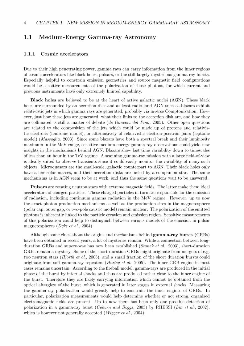
Due to their high penetrating power, gamma rays can carry information from the inner regionsof cosmic accelerators like black holes, pulsars, or the still largely mysterious gamma-ray bursts.Especially helpful to constrain emission geometries and source magnetic field configurationswould be sensitive measurements of the polarization of those photons, for which current andprevious instruments have only extremely limited capability.
Black holes are believed to be at the heart of active galactic nuclei (AGN). These blackholes are surrounded by an accretion disk and at least radio-loud AGN such as blazars exhibitrelativistic jets in which gamma rays are generated, probably via inverse Comptonization. How-ever, just how these jets are generated, what their links to the accretion disk are, and how theyare collimated is still a matter of debate (de Gouveia dal Pino, 2005). Other open questionsare related to the composition of the jets which could be made up of protons and relativis-tic electrons (hadronic model), or alternatively of relativistic electron-positron pairs (leptonicmodel) (Massaglia, 2003). Since some blazars have both a spectral break and their luminositymaximum in the MeV range, sensitive medium-energy gamma-ray observations could yield newinsights in the mechanisms behind AGN. Blazars show fast time variability down to timescalesof less than an hour in the TeV regime. A scanning gamma-ray mission with a large field-of-viewis ideally suited to observe transients since it could easily monitor the variablity of many suchobjects. Microquasars are the small-scale, galactic counterpart to AGN. Their black holes onlyhave a few solar masses, and their accretion disks are fueled by a companion star. The samemechanisms as in AGN seem to be at work, and thus the same questions wait to be answered.
Pulsars are rotating neutron stars with extreme magnetic fields. The latter make them idealaccelerators of charged particles. These charged particles in turn are responsible for the emissionof radiation, including continuum gamma radiation in the MeV regime. However, up to nowthe exact photon production mechanisms as well as the production sites in the magnetosphere(polar cap, outer gap, or two-pole caustic model) remain unclear. The polarization of the emittedphotons is inherently linked to the particle creation and emission region. Sensitive measurementsof this polarization could help to distinguish between various models of the emission in pulsarmagnetospheres (Dyks et al., 2004).
Although some clues about the origins and mechanisms behind gamma-ray bursts (GRBs)have been obtained in recent years, a lot of mysteries remain. While a connection between long-duration GRBs and supernovae has now been established (Stanek et al., 2003), short-durationGRBs remain a mystery. Some of the short-duration GRBs might originate from mergers of e.g.two neutron stars (Hjorth et al., 2005), and a small fraction of the short duration bursts couldoriginate from soft gamma-ray repeaters (Hurley et al., 2005). The inner GRB engine in mostcases remains uncertain. According to the fireball model, gamma-rays are produced in the initialphase of the burst by internal shocks and thus are produced rather close to the inner engine ofthe burst. Therefore they are likely carrying information which cannot be obtained from theoptical afterglow of the burst, which is generated in later stages in external shocks. Measuringthe gamma-ray polarization would greatly help to constrain the inner engines of GRBs. Inparticular, polarization measurements would help determine whether or not strong, organizedelectromagnetic fields are present. Up to now there has been only one possible detection ofpolarization in a gamma-ray burst (Coburn and Boggs, 2003) by RHESSI (Lin et al., 2002),which is however not generally accepted (Wigger et al., 2004).

1.1. MEDIUM-ENERGY GAMMA-RAY ASTRONOMY 5
1.1.2 Nucleosynthesis
When hydrostatic or explosive burning in stars results in the generation of “metals” (elementsheavier than Helium), radioactive nuclei are produced along with stable elements. The decay ofnewly synthesized radioactive nuclei is accompanied by subsequent deexitation through emissionof gamma rays of characteristic energy. From the distribution of such photons of a given lineenergy on the sky one can draw conclusions about that isotopes’ producers and thus the originof the elements that the universe is made of.
Novae, supernovae and late-stage massive stars are the most prominent production sites ofdetectable radioactivity. Those objects expel radioactive “metals” on small enough time scalesso that the decay happens outside the star itself, in an environment of low enough density thatthe resulting gamma ray can reach us.
One of the most challenging questions in gamma-ray astronomy is related to type Ia super-novae. When a white dwarf in a tight binary system accretes enough mass from its companionto exceed the Chandrasekhar mass limit, thermonuclear burning in the core sets in and deto-nates the white dwarf. Supernova Ia explosions are considered to be standard candles due totheir uniform progenitors and consequently are used for distance determinations. Lately, theyhave even been used in cosmology, leading to the conclusion that the expansion of the universeis accelerating (Riess et al., 1998). However, the picture of supernovae Ia as standard candles isnot perfect, and several competing models of their explosion mechanism exist (e.g. Leibundgut ,2000): Does the explosion happen only when the white dwarf exceeds the Chandrasekhar limit,or possibly in some cases while it is still a sub-Chandrasekhar white dwarf? Is the speed of theburning front subsonic (deflagration model) or supersonic (detonation model) or a mixture ofthe two? Since supernovae Ia are rare, a telescope needs an excellent sensitivity (∼100 betterthan COMPTEL) to be able to — within the time frame of a mission — distinguish for tensof supernovae between competing models via the production rates and ejection velocities ofthe individual radioactive isotopes (Milne et al., 2002). Two supernovae Ia were observed withCGRO: SN1991T (distance ∼13 Mpc), which resulted in a marginal detection by COMPTEL(Morris et al., 1995), and SN1998bu (distance ∼9 Mpc), for which only upper limits wherederived (Georgii et al., 2002). A telescope with a significantly improved sensitivity over COMP-TEL to the broadened 847 keV line of the 56Co decay (T1/2 = 77 d) is needed to untangle theexplosion mechanisms which drive type Ia supernovae.
Generally, any detection of a close supernova, irrelevant of the type, by a gamma-ray telescopemore sensitive than its predecessors will greatly enhance the knowledge about supernovae andhelp to constrain the explosion models via the production rate of different elements during theexplosion.
A not-yet detected source of gamma rays are expected to be novae. Through Roche lobeoverflow, a white dwarf can accumulate an outside layer from its main sequence companion ina binary system until hydrogen ignition conditions are reached in this layer. This will lead toa thermonuclear runaway burning, the nova. During this hydrogen burning phase, short-livedβ+-unstable elements such as 13N (T1/2 = 10 m) and 18F (T1/2 = 110 m) are produced andresult in a prompt flash of 511 keV photons as well as a positronium continuum below thisline, which can be detected even before the nova is visible in the optical. The detection of sucha flash would yield constrains on the generation rates of these two radioactive elements, theduration of the emission, and the transport of those elements in the expanding nova envelope(Hernanz , 2004). Other candidates for gamma-ray line emission from novae are 1275 keV from22Na (T1/2 = 2.6 a) and 478 keV from 7Be (T1/2 = 53 d), which can still be detected longafter the actual nova and would allow constraints on the composition of the progenitor and theproduction rate of those elements.
The decay chain of 44Ti (T1/2 = 63 a) with its characteristic 1.157 MeV line is a unique

6 CHAPTER 1. NEW MISSION IN MEDIUM-ENERGY GAMMA-RAY ASTRONOMY
tracer of young supernova remnants. Up to now one source, Cas A (Iyudin et al., 1994), hasbeen detected definitely and another, Vela Junior, marginally by COMPTEL (Schonfelder et al.,2000). The latter has not been detected yet by INTEGRAL (Renaud et al., 2005). Since gammarays have only a small extinction in our galaxy, a sensitive survey for point sources of 44Ti-decaylines should reveal hidden SN remnants and thus stringently constrain the supernovae rate inour galaxy as well as the supernova yields of 44Ti.
26Al (T1/2 = 7.2 105 a) is produced in the cores of massive stars. Wolf-Rayet stars are verymassive stars (m > 30 M�) in a late evolutionary phase which is characterized by heavy massloss. After their original hydrogen-rich envelope has been removed by stellar winds, or sufficientrotation led to diffusion of 26Al into the outer envelopes of the star (e.g. Palacios et al., 2005),26Al is ejected and its decay can be detected by the characteristic 1.809 MeV line. Up to nowno 26Al from an individual Wolf-Rayet star has been detected. For the closest, γ2 Velorum, onlyupper limits have been determined by COMPTEL (Oberlack et al., 2000a) and SPI (Mowlaviet al., 2004). An 26Al measurement of γ2 Velorum would allow to constrain the 26Al outflowfrom and production rate in those stars and thus help to determine the total contribution ofWolf-Rayet stars to the overall detected 26Al.
60Fe (T1/2 = 1.5 106 a), whose decay results in 1.173 and 1.333 MeV gamma rays, should beproduced mainly in massive stars before as well as during their death in a core-collapse supernova,but not be expelled in Wolf-Rayet stars (Palacios et al., 2005). Since 60Fe is mainly ejected bycore-collapse supernovae and some by supernovae Ia, but 26Al is ejected by supernovae, massivestars especially in Asymptotic Giant Branch and Wolf-Rayet phases, and novae, the ratio of 60Feto 26Al should yield constraints to the overall amount of 26Al which is produced in massive stars(e.g. Prantzos, 2004), and all-sky 60Fe maps will trace core collapse supernovae. Up to now onlythe overall line emission of 60Fe and thus the ratio 60Fe/26Al in our galaxy has been measuredby RHESSI (Smith, 2004) and INTEGRAL (Harris et al., 2005), but current instrumentationis not nearly sensitive enough to resolve individual supernovae in the 60Fe line.
Most 26Al is believed to originate in massive stars and core-collapse supernovae. Its half-lifeof T1/2 = 7.2 105 years is long enough for 26Al to accumulate in the interstellar medium aroundregions with massive stars. Due to the relatively short lifetime of massive stars on the mainsequence, late-stage massive stars and core-collapse supernovae are indicators for regions withongoing star formation. Mapping the universe in 26Al with significantly improved sensitivityand/or angular resolution compared to COMPTEL and INTEGRAL will reveal those regionsin much more detail.
Generally, all large scale structures are best imaged if the telescope has a wide field-of-viewand is operated in scanning instead of pointing mode to obtain a smooth, 4π exposure.
1.1.3 Capture, annihilation and deexcitation
When a neutron is captured on hydrogen a characteristic 2.223 MeV gamma ray is produced.Due to the short mean life time of neutrons (918 s), this capture has to happen close to wherethe neutrons are produced mainly via nuclear interactions. Besides solar flares, compact objectssuch as accreting neutron stars and black holes are the most likely sources of such radiation.From the width of the line and a potential redshift the production site close to the compactobject can be deduced: for example gravitational redshift would indicate a production closeto a neutron star atmosphere (Bildsten et al., 1993), a strongly broadened line would indicatethat the neutron capture happened in the hot plasma of the accretion disk, and a narrow linewould indicate that the capture happened in the outer regions of the accretion flow or in theatmosphere of the companion star (e.g. Agaronian and Sunyaev , 1984). Up to now, only oneextra-solar 2.2 MeV line source has been claimed by COMPTEL, but no optical counterpart hasbeen identified (McConnell et al., 1997).

1.1. MEDIUM-ENERGY GAMMA-RAY ASTRONOMY 7
Observations with SPI on INTEGRAL have revealed that a significant amount of the 511keV annihilation radiation of positrons is consistent with emission from or near the galacticbulge (Knodelseder et al., 2005). While the observed weak emission from the galactic disk canbe explained entirely by radioactive beta decay from 26Al and eventually 44Ti, the origin ofthe positrons responsible for the galactic bulge emission remains uncertain. Candidates rangefrom Type Ia supernovae, novae, or low-mass X-ray binaries to light dark matter annihilation(Diehl et al., 2005; Knodelseder et al., 2005; Boehm et al., 2004). Detecting positron emissionfrom any one of the above point source candidates would shed light on the mystery. To achievethis, an excellent angular resolution and sensitivity surpassing that of INTEGRAL/SPI wouldbe required.
After energetic particles, with energies in the tens of MeV/nucleon, inelastically scatteroff and excite matter, deexcitation results in characteristic nuclear interaction lines. Thestrongest gamma-ray lines that are unique signatures of nuclear excitations (as opposed to alsobeing produced in radioactive decays) are those of 12C∗ (4.44 MeV) and 16O∗ (6.13 MeV) (Ra-maty et al., 1979). The strength of the lines should allow inference of the molecular compositionof the ambient matter, of the low energy particles themselves, and potentially of their sources.Up to now nuclear excitation lines have only been conclusively detected from the sun.
1.1.4 Other sources of interest
Nuclei can not only be excited by decay or energetic particle interaction, but also by gammarays. The best-studied case is the Giant Dipole Resonance (GDR), in which the protons andneutrons collectively oscillate around their common center of gravity until the oscillation stopsby either emitting gamma rays or neutrons. The necessary photon energy depends on theradius of the nucleus. For light elements it is between 20 and 30 MeV. Besides the GDR, otherresonance features in the total absorption cross-section of photons on nuclei exist, such as thepygmy dipole resonance (∼7 MeV). Absorption features in the spectra of distant gamma-raysources like AGN that can be attributed to these resonances have recently been found by Iyudinet al. (2005). The absorption lines allow to constrain the column density and eventually thecomposition of the medium by analyzing the peak position, the width and the strength of theabsorption features.
Another source of interest is the origin of the extragalactic and galactic gamma-raybackground. While at lower gamma-ray energies (< 100 keV) the extragalactic backgroundis expected to mainly originate from Seyfert galaxies (e.g. Watanabe and Hartmann, 2001), athigher energies (> 10 MeV) the main contribution to this background is expected to be fromblazars (Stecker and Salamon, 2001). The largest part of the galactic gamma-ray backgroundat lower energies (< 100 keV) seems also to be resolved into point sources (Lebrun et al., 2004).At higher energies (> 10 MeV) most of the galactic background can be explained via interactionof cosmic rays with the interstellar medium, which creates gamma rays through the generationand the decay of π0, bremsstrahlung and inverse Compton scattering (e.g. Strong et al., 2005).Between ∼0.1 and ∼10 MeV the situation is less clear. It still has to be determined how farthe low and high energy sources reach into this regime and how large the contribution of e.g.supernovae Ia is to the background (e.g. Strigari et al., 2005, expects roughly 10%) or if thereare completely different mechanisms at work, e.g. like a dark matter annihilation contributionto the cosmic gamma-ray background (Ahn and Komatsu, 2005). Thus one of the main tasksof a future medium energy gamma-ray telescope is to resolve as much as possible of the diffusegalactic and extragalactic background into point sources and to measure the remaining diffuseemission with far higher accuracy.
Besides the main motivations for improved observations in medium-energy gamma-ray as-tronomy outlined above, there is of course the unexpected, which awaits its discovery with a

8 CHAPTER 1. NEW MISSION IN MEDIUM-ENERGY GAMMA-RAY ASTRONOMY
future mission which significantly surpasses the sensitivity of COMPTEL and INTEGRAL!
1.2 Instrumentation for medium-energy gamma-ray astronomy
The energy band from a few hundred keV up to several tens of MeV, in which initially Comptonscattering is the dominating interaction mechanism followed by the onset of pair creation (seecross-sections in Figure 1.1), is one of the hardest to explore. The atmosphere is almost opaqueto MeV photons and therefore high-altitude balloon or satellite missions are needed for itsexploration. It is ironic that two properties of the MeV regime that make observations at theseenergies particularly rewarding — the high penetration power and the information carried innuclear lines — also make this regime particularly challenging for observers. Around 2 MeV,depending on the material, the interaction probability reaches a minimum and a significantamount of material (∼40 g/cm2) is needed to stop a sufficient portion of the gamma rays inthe active detector material. But up to a few MeV the most demanding challenge is the highinternal instrumental background induced by the time-variable space radiation environment.This generally leads to very low signal-to-background ratios. Thus the single most importantfeature of any future mission in medium-energy gamma-ray astronomy is improved backgroundprevention and rejection. This can be achieved by the applied gamma-ray measurement processitself as well as by detector design and sophisticated data analysis techniques.
The following sections describe the different detector concepts which can be used for gamma-ray imaging in this energy band. Most of the presented detectors are surrounded by an anti-coincidence shield to reject parts of the cosmic and atmospheric background radiation. Suchshields are either made of thin plastic to reject charged particles only or of significantly heaviermaterial (CsI, BGO) to reject also photon components. They will not be discussed further inthis chapter.
1.2.1 Spatial and temporal modulation
One way of determining the origin of gamma rays is by obscuring parts of the field-of-viewof the detector, either permanently or in a well-defined temporal manner. From the detectedmodulated signal and the knowledge of the obscuration scheme, the original distribution of thephotons can be recovered by means of deconvolution.
The simplest system is a collimator. Only those photons can reach the detector which are notblocked by the collimator. One recent example is the Hard X-ray detector (HXD) aboard Astro-
Energy [keV]10 210 310 410 510 610 710
]2cr
oss
sect
ion
[cm
-410
-310
-210
-110
1
10
210
Photo effect
Compton scattering
Pair creation
Rayleigh scatteringFigure 1.1: Cross-section for pho-ton interactions in Silicon in theMeV range. The four dominatinginteraction mechanisms are photoeffect, Compton scattering, paircreation and Rayleigh scattering.

1.2. INSTRUMENTATION FOR MEDIUM-ENERGY GAMMA-RAY ASTRONOMY 9
Figure 1.2: The basic design of acoded mask telescope as used onINTEGRAL and on SWIFT: Thegamma rays have to pass through amask. From the resulting shadow-gram on the detector, the origin ofthe photons can be reconstructed.
E2/Suzaku (Inoue et al., 2003). However this simple system has one large drawback: it providesonly a small field-of-view and the background determination requires off-source pointings whichreduce the observation time.
The next step is a coded mask system. Different sources on the sky cast different shadowsof the mask onto a spatially resolving detector system (see Figure 1.2). From the measuredshadowgrams and the knowledge of the mask, the original distribution of the photons can bedeconvolved (Caroli et al., 1987). Currently three coded masks instruments (SPI, IBIS andJEM-X) operate aboard INTEGRAL (Winkler et al., 2003), from which two, the imager IBISand the spectrometer SPI, extend into the MeV range. Coded masks are also used for the burstalert telescope (BAT) aboard SWIFT (Gehrels et al., 2004) and planned for the EXIST hardX-ray telescope (Grindlay et al., 2003).
Another approach is to rotate two collimators above a monolithic detector and derive theinformation of the origin of the photons through Fourier analysis of the temporally encodedinformation (Hurford et al., 2002). This approach is used by the solar spectroscopic imagerRHESSI (Lin et al., 2002).
Coded masks and rotation modulation collimators have several limiting factors: First, it isnot possible to derive a unique origin for one single photon, but one needs enough events to pro-duce a complete shadowgram or enough events to generate the complete temporal information.Second, once the event is registered in the detector it is not possible to further analyze it andpotentially identify it as background as long as only simple detectors are used. Thus generallythe background level is high in this approach. Third, those systems are best suited for pointsources and small emission regions; it is more difficult to image large scale structures. Finally,multiplexing approaches are better suited for lower energies, because they need a decent amountof photons to deconvolve the image and at higher energies require rather thick masks to blockthe photons.
Nevertheless, since those systems allow for a high angular resolution and utilize relativelysimple detector concepts, they are currently wide-spread in gamma-ray astronomy.
1.2.2 Single event detector systems
A completely different way of reconstructing the origin of photons becomes feasible at energiesabove a few hundred keV with the onset of Compton scattering and pair creation. Recordingenergies and directions of the secondary/scattered particles allow to retrieve origin, energy andsometimes polarization of the original photon.

10 CHAPTER 1. NEW MISSION IN MEDIUM-ENERGY GAMMA-RAY ASTRONOMY
�t
Figure 1.3: Comparison of the different Compton telescopes: The left figure shows the classical COMPTEL typeinstrument. It comprises two detector planes. The first one is the scatterer (D1) and the second is the absorber(D2). The planes have a large distance in order to measure the time-of-flight of the scattered gamma-ray. Thecentral picture shows a Compton telescope consisting of several thick layers in which the photon undergoesmultiple Compton scatterings. The redundant scatter information allows to determine the direction of motionof the photon. The figure on the right shows an electron tracking Compton telescope like MEGA. The trackerconsists of several layers, thin enough to track the recoil electron. The scattered photon is stopped in a seconddetector which encloses the tracker. The track of the electron determines the direction of motion of the photon.The illustrations are not to scale.
1.2.2.1 Compton Telescopes
Compton scattering is the dominant interaction process between ∼200 keV and ∼10 MeV (de-pending on the scatter material). If one measures the position of the initial Compton interac-tion, energy and direction of the recoil electron as well as direction and energy of the scatteredgamma-ray, then the origin of the photon can be identified. The final accuracy depends onseveral factors, which are extensively discussed in Section 2.2.
The key objective for a Compton telescope is to determine the direction of motion of thescattered gamma-ray. For this problem three solutions exist which distinguish the three basictypes of Compton telescopes (see Figure 1.3).
In COMPTEL (Figure 1.3 left) the two detector systems, a low Z scatterer, where the initialCompton interaction takes place, and a high Z absorber, where the scattered gamma ray isstopped, are well separated so that the time-of-flight of the scattered photon between the twodetectors can be measured. Thus top-to-bottom events can be distinguished from bottom-to-topevents. With COMPTEL it was not possible to measure the direction of the recoil electron, soan ambiguity in the reconstruction of the origin of original photon emerged: the origin couldonly be reconstructed to a cone. This ambiguity has to be resolved by measuring several photonsfrom the source and by image reconstruction (details see Chapter 5).
Several of the instrument concepts currently under consideration for an Advanced ComptonTelescope (ACT) (Boggs et al., 2005) will detect more than one Compton interaction per photon(Figure 1.3 center). From the resulting redundant information the ordering of the interactionscan be retrieved. A detailed discussion of this approach is given in Chapter 4. Representativesof this group of Compton telescopes are NCT (Boggs et al., 2004), LXeGRIT (Aprile et al.,2000) or the thick Silicon concept described by (Kurfess et al., 2004).
In contrast to COMPTEL and most ACT concepts, a third group of detectors is capable ofmeasuring the direction of the recoil electron (Figure 1.3 right). This enables the determinationof the direction of motion of the scattered photon and allows to resolve the origin of the photonmuch more accurately: the Compton cone is reduced to a segment of the cone, whose lengthdepends on the measurement accuracy of the recoil electron. The main representatives of this

1.2. INSTRUMENTATION FOR MEDIUM-ENERGY GAMMA-RAY ASTRONOMY 11
�
�
Figure 1.4: Basic design of a pair telescope: it com-prises two detector systems, a tracker/converter inwhich the direction of the electron and positron aremeasured and a calorimeter which measures the en-ergy of the particles.
Figure 1.5: Basic design of a crystal diffraction lens:Gamma rays are Laue-diffracted in a lens and focusedon a small detector
group are MEGA, which will be discussed in this work, and TIGRE (Bhattacharya et al., 2004).Compton telescopes have the advantage that only a few photons are needed to recover the
position of sources, depending on background conditions and quality of the events. They arealso inherently sensitive to polarization, especially if the detector allows to measure photonsunder large Compton scatter angles and at low energies (details see 2.2.3). Furthermore theycan easily have a very large field-of-view.
However for all those advantages a price must be paid: The original photon is measuredvia several individual measurements at different interaction positions. Each of these introducesmeasurement errors which are propagated into the recovery of the origin and energy of thephoton. Moreover, modern versions of Compton telescopes are extremely complex with hundredsof thousands of channels, which all need to provide excellent energy and position information. Inaddition, the complexity of the measurement process requires non-trivial techniques to find thedirection of motion of the photons (see Chapter 4) and the origin of the photons (see Chapter5). Finally, a fundamental limit for the angular resolution of Compton telescopes exists, sincethe initial (pre-scattering) momentum of the target electron cannot be determined (see Section2.2.6).
1.2.2.2 Pair-Tracking Telescopes
Compared to Compton scattering, pair production enables a significantly more straight-forwarddetermination of the origin of the photon. In its basic design a pair telescope consists of twodetectors: A converter and an absorber (compare Figure 1.4).
The converter consists of layers of high-Z conversion foils combined with position sensitivedetectors to determine the tracks of the generated electron and positron. While semiconductorsare used in modern-day pair telescopes like GLAST (Gehrels and other , 1999) and AGILE(Tavani et al., 2003), in previous pair telescopes like EGRET (Kanbach et al., 1988) a sparkchamber was used for this task. The energy measurement happens in the bottom absorber, thecalorimeter. From the directions and energies of electron and positron the origin of the incomingphoton can easily be determined (for more details see Section 2.3). Even if the photon-inducedshower is not contained in the detector, an analysis of the morphology of the tracks allows toroughly determine the energy of the initial photon.
Pair telescopes are a simple and efficient approach to determining the origin of gammarays above ∼10 MeV. However, the use of conversion foils, which are necessary to obtain high
12 CHAPTER 1. NEW MISSION IN MEDIUM-ENERGY GAMMA-RAY ASTRONOMY
efficiencies, limits the angular resolution and energy measurement at low energies. Thus to givereasonable performance in the medium-energy gamma-ray regime a pair telescope should notcontain such foils.
1.2.3 Focusing gamma-rays
The latest development for detecting gamma-rays in medium-energy gamma-ray astronomy arelenses. They enable focusing, which is the standard approch at lower energies, also in the gammaregime. Compared to the previously presented concepts, they allow the separation of collectionand detection area, and thus dramatically reduce the background.
1.2.3.1 Laue lens
Focusing gamma-rays can be achieved via Laue-diffraction on crystal planes. Compared toBragg-diffraction, which happens on or near the surface of the material, Laue diffraction meansthat the gamma rays pass through the lens and are diffracted in the volume of the crystal — ifthey satisfy the Bragg-relation:
2d sin θ = nλ (1.1)
Here d is the crystal plane spacing, θ the diffraction angle, n the reflection order and λ thewavelength.
Many such crystals are combined to form a gamma-ray lens. This technique has been initiallydemonstrated for astrophysics by the CLAIRE balloon-flight (Halloin, 2003) and is intended tobe used on the envisioned MAX space telescope (von Ballmoos et al., 2004). The Laue lens onMAX consists of a ring of crystals, which are oriented in a way that they diffract the radiationto a small focal spot on the detector. In order to increase the effective area, the lens has severalrings, which differ in their material (different crystal plane spacings) and/or their orientation(diffraction of higher order) to focus more gamma rays of a given energy onto the detector.Figure 1.5 illustrates the basic concept.
Gamma-ray lenses have one important advantage over non-focusing telescopes: the detectionvolume, which is basically the focal spot, is much smaller than the collection area formed bythe lens. Thus only a very small detector volume is necessary, which dramatically reduces theintrinsic background, which is a sensitivity-limiting factor for other gamma-ray telescopes.
But this advantage comes at the expense of a very narrow field of view (below one arcmin).Also, since the diffraction band width of any individual crystal is only a few keV, the instrument’senergy range is roughly proportional to the number of crystals needed and thus to the overallinstrument complexity. A viable mid-size instrument like MAX would be capable of viewing2-3 energy bands, each of which would be roughly 100 keV wide. Moreover, such a lens hasonly limited imaging capabilities with its field-of-view. With current technology, lenses could beapplied to photon energies up to a few MeV.
1.2.3.2 Fresnel lenses
Another approach that currently exists on paper only is to focus gamma rays using phase Fresnellenses (Skinner , 2001). The refraction index for gamma-rays in matter is slightly lower than 1and thus allows focusing. Besides the drawbacks already mentioned for the Laue lens, a Fresnellens would require a large focal length around 109 m, depending on the energy of the photons.However, one would obtain a superior angular resolution near the diffraction limit in the μarcsecregion, an efficiency close to 100%, and true imaging.

1.3. MEGA - A TELESCOPE FOR MEDIUM-ENERGY GAMMA-RAY ASTRONOMY 13
ComptonPair
Anticoincidence shield
scatteringcreatingγ−photonγ−photon
α
Inst
rum
ent o
vera
ll he
ight
: 1.3
m
Instrument overall width: 1.2 m
Reducedevent circle
ϕ
Calorimeter
Tracker
Figure 1.6: Baseline design and measurement princi-ple of the full MEGA telescope. The recoil electronsfrom Compton scattering as well as the pair creationproducts are tracked in a stack of Silicon strip detec-tors and the secondary particles are stopped in the CsIcalorimeter.
Figure 1.7: MEGA prototype: The tracker (centralbox) is surrounded by 20 calorimeters
1.3 MEGA - A telescope for medium-energy gamma-ray astron-omy
Defining the medium-energy gamma-ray energy band from a few hundred keV up to tens of MeV,the number of available telescope candidates reduces: Coded mask systems would need massivemasks to completely stop these photons and could probably only provide a very small field ofview. Laue lenses have not been seriously considered above a few MeV. The natural candidateswould be Compton-scattering or pair-creation telescopes. However, neither a Compton nor apair telescope can cover the whole energy range, thus the perfect solution is a hybrid telescope:an electron-tracking Compton telescope which is automatically also a low-energy pair telescope(Figure 1.6).
The idea of constructing such a telescope as successor of COMPTEL and EGRET (lowenergies only) has been pursued at the Max-Planck-Institut fur extraterrestrische Physik sincethe mid 1990s and culminated in the successful calibration of the MEGA prototype (Figure 1.7)in 2003, accompanied by detailed studies of a satellite version.
Like all previous successful Compton and pair telescopes, MEGA consists of three detectorsystems, a scatterer/converter/tracker, a calorimeter, and a surrounding anti-coincidence shield.The tracker has several tasks. First, it has to act as a Compton scattering and pair creationmedium. Therefore the material requires a large cross-section for those interactions and lowDoppler-broadening (details see 2.2.6) — for both reasons a low Z material is preferred. Second,it has to measure the direction of the secondary electrons and positrons as well as their energyvery accurately. The logical choice, which provides good position and energy resolution is astack of thin double-sided Silicon strip detectors. The prototype has 11 layers, each of whichconsists of nine 6×6 cm2 wafers. The individual wafer is 0.5 mm thick and has 128 orthogonal pand n strips on opposite sides (0.47 mm pitch). A potential tracker for a satellite version wouldbe a factor of four larger in area and a factor three deeper (32 layers with 36 wafers).
The lower hemisphere of the tracker is surrounded by calorimeters. Their main purpose is tostop all secondary particles and measure the interaction position as well as the deposited energy.Thus it should be built of high-Z material and have good position and energy resolution. Thecalorimeter of the prototype consists of 20 modules of three types: 8 cm deep ones at the bottom,

14 CHAPTER 1. NEW MISSION IN MEDIUM-ENERGY GAMMA-RAY ASTRONOMY
4 cm deep at the lower side and 2 cm deep calorimeters at the upper side. The depth correspondsto the necessary stopping power for on-axis incident photons: Small Compton scatter anglescorrespond to a high energy of the scattered photon and thus require more material for theirabsorption. Each module is built from 10×12 CsI(Tl) scintillator bars with a cross-section of5×5 mm2. The possible satellite version also uses such CsI modules, only the side walls have auniform thickness of 4 cm.
Finally the whole detector is surrounded by an plastic anti-coincidence shield to rejectcharged particles of cosmic and atmospheric origin.
A more detailed discussion of the prototype and its calibration can be found in Chapter 6and even more detail is given in Andritschke (2006). Additional information about a potentialsatellite version of MEGA can be found in Chapter 10.
Chapter 2
Interaction processes in a trackingCompton and pair telescope
In order to develop reliable and accurate reconstruction techniques for the measured events,it is essential to first gain a detailed understanding of the photons’ possible interactions inthe detector. In keeping with the type of instrument discussed in this work, photo absorptionis mentioned only in the context of fully contained Compton scattering events, and Rayleighscattering is ignored since its effects in a MEGA-type telescope are negligible.
All relevant photon interactions — photo-absorption, Compton scattering, and pair produc-tion — can be detected only via interactions resulting in energetic electrons and positrons inthe instrument. Thus a detailed understanding of electron interactions constitutes the necessaryfoundation for a detailed discussion of the different photon detection processes (Section 2.1).Sections 2.2 and 2.3 discuss Compton and pair interactions. Using the idealized interactionsof gamma-ray photons with matter as a starting point, each section subsequently describes themultitude of effects that occur in a real instrument.
2.1 Interactions of electrons with matter
When an electron (or positron) passes through matter, it interacts with the atoms’ Coulombpotentials: It undergoes many small-angle scatterings (Moliere scattering) and loses energymostly via ionization and bremsstrahlung.
2.1.1 Moliere scattering of electrons
The process of multiple small-angle scatters of electrons on Coulomb potentials is called Molierescattering. The change in the flight direction is described by Moliere theory (for an overviewsee Bethe, 1953). The scatter angle distribution can be approximated by a Gaussian (ParticleData Group, 2004, see also Figure 2.1). The width of the angular distribution, projected on ascattering plane, is given by:
δ0,proj =13.6MeV
βcp
√r
R0
(1 + 0.038 ln
r
R0
)(2.1)
Here βcp = E2e+2EeE0
Ee+E0is the velocity times the momentum of the electron, Ee is the electron
energy, E0 the rest energy of the electron, R0 the radiation length in the material (9.35 cm forSilicon), and r is the straight path length (i.e. the straight line between start and end points) ofthe electron in the material. The non-projected width of the angular distribution δ0, which isbasically given by
√2 · δ0,proj, is shown for Silicon in Figure 2.2. The simulation was performed
15

16 CHAPTER 2. INTERACTION PROCESSES
with Geant3 for normal incidence and the electrons were passing through one slab of Silicon(500 μm thick). Profiles for 1 MeV and 5 MeV electrons are shown in Figure 2.1.
]°Projected scatter angle [0 50 100 150
(no
rmal
ized
)°
even
ts/
0
0.5
1
]°Projected scatter angle [0 50 100 150
(no
rmal
ized
)°
even
ts/
0
0.5
1
Figure 2.1: Typical Moliere profiles at 1 MeV (left) and 5 MeV (right) as simulated with Geant3. After passing500 μm of Silicon, the projected scatter angle of the electron has roughly a Gaussian shape. Only those electronsat 1 MeV which reverse their direction (scatter angles > 90◦) do no longer follow the Gaussian approximation.They collect in a tail of the distribution at larger projected scatter angles.
Total electron energy [keV]2000 4000 6000 8000 10000
]° 6
8% c
onta
inm
ent a
ngle
[
0
20
40
60Figure 2.2: Geant3 simulation of the width ofthe angular distribution for electrons passingthrough 500 μm of Silicon (one tracker layerfor MEGA). Given is the cone opening anglearound the original direction, enclosing 68%of all events. This corresponds to
√2 · δ0,proj
of the width given in Equation 2.1.
Considering electron tracks in MEGA’s stack of Si strip detectors, Moliere scattering hasfour consequences:
1. Given the geometry of the MEGA tracker (distance between layers 1 cm, pitch of the stripdetector 470 μm), the directions of a track element (line between two interaction points)can be resolved up to 3◦ at normal incidence. This value is smaller than δ0 for electronenergies below 21 MeV. Thus almost all electron-direction measurements in the tracker arelimited by Moliere scattering. Of course switching to thinner Silicon layers would improvethe situation a bit. But with e.g. 300 μm thick wafers, the limit is still at 15 MeV, whichis not a significant improvement.
2. Since the electron deposits and thus loses energy along the track, and δ0 increases withdecreasing energy, the average scatter angle increases along the path of the electron. Thisis one criterion for determining the direction of motion of the electron.
3. The given widths of the angular distributions are for electrons which pass one layer ofSilicon completely. This is normally not the case for the interaction in the first layer,where the Compton scattering happens. Here, the recoil electron does not need to passthe whole layer. As a consequence, the effect of Moliere scattering is reduced by typically50% for the electron emerging from the conversion layer. The same holds for pair creation.
2.1. INTERACTIONS OF ELECTRONS WITH MATTER 17
4. Finally, from the above three points follows that the direction of the original electron inthe MEGA energy range is best determined only from the first and the second interactionpoints.
2.1.2 Energy loss of electrons in matter
Six processes contribute to the energy loss of electrons and positrons, two of which dominatein a MEGA-type Silicon tracker: ionization at low energies, bremsstrahlung at high energies.The electron energy for which both loss rates are equal is called the critical energy. It canbe approximated by Ec = (800 MeV)/(Z + 1.2) ≈ 53 MeV for Si (Berger and Seltzer , 1964).Electron and positron interactions in MEGA are thus dominated by ionization. A welcomeconsequence of this is that MEGA tracks are not going to be “polluted” by a significant amountof additional bremsstrahlung hits, making the tracking much easier than for higher energygamma-ray telescopes like GLAST. Other energy loss mechanisms are Møller scattering forelectrons, Bhabha scattering for positrons respectively, positron annihilation before the positronis completely stopped, and δ-rays (knock-on electrons) (see e.g. Particle Data Group, 2004).None of the latter play an important role for MEGA.
Total electron energy [keV]0 1000 2000 3000 4000 5000
Mea
n en
ergy
dep
osit
[keV
]
0
100
200
300
400
MIP character of electron
Absorption in one wafer
Increase of energy deposit at lower energies
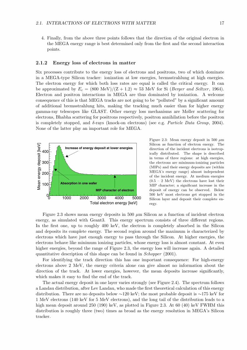
Figure 2.3: Mean energy deposit in 500 μmSilicon as function of electron energy. Thedirection of the incident electrons is isotrop-ically distributed. The shape is describedin terms of three regions: at high energies,the electrons are minimum-ionizing particles(MIPs) and their energy deposits are (withinMEGA’s energy range) almost independentof the incident energy. At medium energies(0.5 – 2 MeV) the electrons have lost theirMIP character; a significant increase in thedeposit of energy can be observed. Below500 keV most electrons get stopped in theSilicon layer and deposit their complete en-ergy.
Figure 2.3 shows mean energy deposits in 500 μm Silicon as a function of incident electronenergy, as simulated with Geant3. This energy spectrum consists of three different regions.In the first one, up to roughly 400 keV, the electron is completely absorbed in the Siliconand deposits its complete energy. The second region around the maximum is characterized byelectrons which have just enough energy to pass through the Silicon. At higher energies, theelectrons behave like minimum ionizing particles, whose energy loss is almost constant. At evenhigher energies, beyond the range of Figure 2.3, the energy loss will increase again. A detailedquantitative description of this shape can be found in Schopper (2001).
For identifying the track direction this has one important consequence: For high-energyelectrons above 2 MeV, the energy criteria alone can give almost no information about thedirection of the track. At lower energies, however, the mean deposits increase significantly,which makes it easy to find the end of the track.
The actual energy deposit in one layer varies strongly (see Figure 2.4). The spectrum followsa Landau distribution, after Lev Landau, who made the first theoretical calculation of this energydistribution. There are no deposits below ∼120 keV; the most probable deposit is ∼175 keV for1 MeV electrons (140 keV for 5 MeV electrons), and the long tail of the distribution leads to ahigh mean deposit around 250 (190) keV, as plotted in Figure 2.3. At 60 (40) keV FWHM thisdistribution is roughly three (two) times as broad as the energy resolution in MEGA’s Silicontracker.

18 CHAPTER 2. INTERACTION PROCESSES
Deposited electron energy [keV]0 100 200 300 400 500
even
ts/k
eV (
norm
aliz
ed)
0
0.5
1 Most probable deposit
Mean deposit
Deposited electron energy [keV]0 100 200 300 400 500
even
ts/k
eV (
norm
aliz
ed)
0
0.5
1 Most probable deposit
Mean deposit
Figure 2.4: Deposit profiles for 1 MeV (left) and 5 MeV (right) electrons after passing 500 μm Silicon as simu-lated with Geant3. The direction of the original electron was isotropically distributed. The shape is a Landau-distribution, with a very long tail. Thus, the mean deposit with 256 (190) keV is significantly larger than themost probable deposit with 175 (145) keV.
2.2 Compton scattering
In 1923 Arthur H. Compton (1892-1962) discovered that X-rays can be scattered on electronsduring their passage through matter and that there exists a relation between the scatter angleand the initial and final wavelength of the photon (Compton, 1923), which was later calledCompton equation (Equation 2.6). A schematic drawing of the Compton effect is shown inFigure 2.5, which also serves as an illustration of notations used throughout this work1.
In the following, first three fundamental aspects of (idealized) Compton scattering are de-scribed: Scatter kinematics, scatter probabilities as function of scatter angles, and the impactof photon polarization on the scatter cross-section are discussed in Sections 2.2.1 – 2.2.3. Thelatter includes an introduction to Compton polarimetry. These three sections are followed bydetailed explanations of all the ways in which a real-life detector deviates from the ideal, andthe consequences this has for the determination of the incident photons’ direction and energy.Section 2.2.4 describes the consequences of incomplete or missing information about energies ordirections, Section 2.2.5 introduces measures for the angular resolution of the instrument anddiscusses the impact of energy and position accuracy on the angular resolution. The influence
1For a complete list of frequently-used notations see also Appendix A.
� �
�
Ei
Eg
Ee
Photon scatter cone
Electron scatter cone
ee
eg
ei
Ei Energy of initial gamma rayEe Energy of the recoil electronEg Energy of the scattered gamma rayE0 Rest energy of the electronErel
e Total relativistic energy of the electronϕ “Compton scatter angle” of the gamma rayε “Electron scatter angle” of the recoil electronϑ Total scatter angle ei Direction of the initial gamma ray ee Direction of the recoil electron eg Direction of the scattered gamma ray
Figure 2.5: Compton-scattering and all notations. Undulated lines represent photons, straight lines electrons.The photon scatter cone represents all possible origin directions of the photon in case the direction of the electroncould not be measured, the electron scatter cone represents the possible origins in case the scattered photons’direction could not be measured.

2.2. COMPTON SCATTERING 19
of a bound electron’s initial energy and momentum on the instrument’s angular resolution isdiscussed in Section 2.2.6.
2.2.1 Kinematics
The underlying scatter problem can be described in terms of conservation of energy and mo-mentum of photon and electron:
Ei + Ereli,e = Eg + Erel
e (2.2)
pi + pi,e = pg + pe (2.3)
The initial energy Ereli,e and momentum pi,e of a bound electron are unknown. In the following
it is assumed that the electron is at rest, i.e. its initial energy is its rest energy E0 and itsmomentum pi,e is zero. However, this unavoidable approximation has a consequence, the so-called Doppler-broadening limit to a Compton telescope’s angular resolution, which is explainedin Section 2.2.6.
Application of the relativistic energy-momentum-relation Erele =
√E2
0 + p2ec
2 = Ee +E0 andthe relation between energy and momentum of photons Eg = pgc leads to the following equationsfor direction and energy of the initial photon:
ei =
√E2
e + 2EeE0 ee + Eg eg
Ee + Eg(2.4)
Ei = Ee + Eg (2.5)
In his original work of 1923 Compton could not measure the direction of the recoil electron —he could only measure the direction and energy change of the scattered gamma ray. He foundthe following relation between energies and scatter angle ϕ, which was later called Comptonequation:
cos ϕ = 1 − E0
Eg+
E0
Eg + Ee(2.6)
In order to get a mathematically valid Compton scatter angle ϕ — the arccos has the domain[−1; 1] — Ee and Eg have to comply with the following constraints:
E0Ei
2Ei + E0< Eg < Ei for the scattered photon
0 < Ee <2E2
i
2Ei + E0for the recoil electron (2.7)
These constraints correspond to backscattering of the gamma ray (energy of the photon reachesits minimum) and no scattering at all (Eg = Ei).
Equations similar to 2.6 exist for the scatter angle ε of the recoil electron and the total angleϑ between the directions of scattered photon and recoil electron:
cos ε =Ee(Ei + E0)
Ei
√E2
e + 2EeE0
(2.8)
cos ϑ =Ee(Eg − E0)
Eg
√E2
e + 2EeE0
(2.9)
Obviously, ε can take values between 0◦ (back scattering) and 90◦ (forward scattering, Ee →0) for fixed Ei. For the limit of (almost) no energy transfer to the electron, ϑ is equal to90◦. In the case of small Ei (< E0), the total scatter angle rises monotonely with increas-ing Ee. If the incident photon’s energy exceeds E0, ϑ as a function of Ee first falls towards
arccos(
Ei−E0Ei+2E0
√E2
i −E20
E2i +2E0Ei
)and then rises again. Finally, in the case of back scattering, ϑ is
equal to 180◦.

20 CHAPTER 2. INTERACTION PROCESSES
2.2.2 Cross-sections
A few years after Compton’s discovery, Klein and Nishina (1929) derived the differential Comp-ton cross section
(dσdΩ
)for unpolarized photons scattering off unbound electrons:(
dσ
dΩ
)C, unbound, unpol
=r2e
2
(Eg
Ei
)2(Eg
Ei+
Ei
Eg− sin2 ϕ
)(2.10)
Here re is the classical electron radius. The above equation is also called the unbound Comptoncross section since the electron is assumed to not be bound to an atom and therefore to be atrest. Because this is not the case for any detector material used in Compton telescopes today,the Klein-Nishina cross section constitutes an approximation. Figure 2.6 illustrates the angulardependence of the Compton cross section for 0.1, 1 and 10 MeV photons.
��������������
����
�����
���
�������
�������
Figure 2.6: Klein-Nishina cross-section as a function of the Comp-ton scatter angle ϕ for differentenergies: The higher the energy,the smaller the average Comptonscatter angle — i.e. the strongeris the forward scattering.
2.2.3 Polarization
Compton scattering also preserves the polarization information of linearly polarized photons upto a certain degree. If the initial gamma ray is polarized, then the following differential crosssection applies: (
dσ
dΩ
)C, unbound, pol
=r2e
2
(Eg
Ei
)2(Eg
Ei+
Ei
Eg− 2 sin2 ϕ cos2 χ
)(2.11)
Here χ is the azimuthal or polar scatter angle.The polarization signature of the incident linearly polarized photons is reflected in the prob-
ability distribution of the azimuthal scatter angle, which can be derived from Equation 2.11:
P (χ) = P0 + A cos (2 (χ − χ0 + π/2)) (2.12)
Here χ0 is the direction of the original polarization vector.In qualitative terms, this polarization dependence can be described as follows (compare
Equation 2.11):

2.2. COMPTON SCATTERING 21
]° [χAzimuthal scatter angle
0 90 180 270 360
Cou
nts
0
50
100
150
200
250
P(max) P(min)
A
0P
Pol
ariz
atio
n
0χan
gle
Figure 2.7: Expected polarization sig-nal for a 100% polarized gamma-raybeam: The distribution of the az-imuthal scatter angle χ is of the formP (χ) = P0 + A cos (2 (χ − χ0 + π/2))and μ = A/P0 is the modulation. Theminimum of the signal defines the planeof polarization of the original photons.
• The scattered photons tend to scatter at right angles to the original polarization vector,minimizing the term −2 sin2 ϕ cos2 χ.
• At higher energies and therefore lower average Compton scatter angles, the modulation ofthe azimuthal distribution is reduced.
• For small and very large Compton scatter angles ϕ the detectable polarization signatureis weak (sin2 ϕ is close to zero).
The polarization response of a detector can be described in terms of a quality factor μ (alsocalled modulation). It is defined as the ratio between the amplitude A and the offset P0 of theazimuthal scatter angle distribution. For a 100% linearly polarized beam of gamma rays, it isgiven by the following equation (see Figure 2.7 for a definition of variables):
μ =P (max) − P (min)P (max) + P (min)
=A
P0(2.13)
The modulation as a function of incident energy Ei and scatter angle ϕ is shown in Figure2.8. The maximum of the modulation shifts from ϕ = 90◦ for low energies to ϕ = 54◦ at 5 MeVand ϕ = 45◦ at 10 MeV.
In a quest to detect polarization of e.g. gamma-ray bursts, of course special selection criteriamust be applied to detected events to maximize an instrument’s polarization sensitivity. The
]° [ϕ020406080100120140160180
[MeV]
iE
01
23
45
μ
0
0.2
0.4
0.6
0.8
1
Figure 2.8: Modulation as afunction of incidence energyEi and Compton scatter an-gle ϕ as derived from theKlein-Nishina cross section.The thick black line indi-cates the maximum of mod-ulation for a given incidentenergy. The thin lines indi-cate levels of constant mod-ulation. Each real polarime-ter aims at getting as closeas possible to these ideal val-ues.

22 CHAPTER 2. INTERACTION PROCESSES
Compton-scatter polarization signature is most pronounced at medium scatter angles and lowerenergies. For a deeper insight into the basic principles of Compton polarimetry, refer to Leiet al. (1997).
2.2.4 Incomplete measurement
In the previous sections ideal Compton telescopes have been discussed. However, when workingwith any real-life instrument, several additional aspects have to be taken into consideration. Ifthe energies of the recoil electron Ee and the scattered photon Eg as well as their directions ee and eg are determined with high accuracy, the origin of the photon can be calculated usingEquation 2.4. However, even if not all four parameters are measured (or only measured with alarge error) it is still possible to constrain the origin and energy of the photon.
2.2.4.1 Missing or uncertain directions
COMPTEL, as a first-generation Compton telescope, was unable to measure the direction of therecoil electron. An equation describing the possible origins of the photon for this case can bederived. In the following, the z-axis is assumed to be parallel to the scattered photon’s direction.
The Compton scatter angle ϕ can be written as:
cos ϕ = ei ◦ eg = ei,z · eg,z = ei,z (2.14)
With the constraint || ei|| = 1 follows:
e2i,x + e2
i,y = 1 − cos2 ϕ = sin2 ϕ (2.15)
This equation describes a circle in the x-y-plane with radius r = sinϕ. With the reparametriza-tion ei,x = r sin t and ei,y = r cos t one obtains for the origin of the gamma ray:
ei (t) =
⎛⎝ sin ϕ sin t
sin ϕ cos tcos ϕ
⎞⎠ ∀ t ∈ [0, 2π] (2.16)
Thus the incident direction of the detected gamma ray can be restricted to a cone whoseopening angle is the Compton scatter angle ϕ and whose axis points in direction of the scatteredphoton (Figure 2.5). However, the origin of the photon can no longer be determined uniquely.The resulting ambiguity has to be resolved by image reconstruction techniques (see Chapter 5)and is only possible if a sufficient amount of photons (depending on background conditions) hasbeen measured. Such events constitute the majority of interactions in the MEGA telescope atlow energies, where no electron tracks can be acquired.
An equation similar to 2.16 can be derived if the electron scatter angle is well known, butno information about the photon scatter angle is present. If the z-axis points in direction of therecoil electron direction, one gets:
ei (t) =
⎛⎝ sin ε sin t
sin ε cos tcos ε
⎞⎠∀ t ∈ [0, 2π] (2.17)
Again the origin direction of the gamma ray can be restricted to a cone, now with openingangle ε (electron scatter angle) and pointing into the direction of the recoil electron (Figure2.5). In the MEGA detector, the measurement of the energy of the scattered gamma ray isalways accompanied by a measurement of its direction that is at least as accurately known as

2.2. COMPTON SCATTERING 23
the electron track direction. Consequently, this event type cannot be found in the data of theMEGA instrument and will not be discussed further.
Even if a photon has been completely absorbed and the electron’s energy was sufficient togenerate a track, the direction of the recoil electron can still only be measured to within the limitof Moliere scattering (see Section 2.1). Combining the well-determined Compton cone and theless accurately known electron cone leads to the typical arc-like distribution of possible originsof such a photon on the sky (see e.g. Figure 5.3). This is the main event type of the MEGAdetector at medium (2-10 MeV) energies.
2.2.4.2 Missing or incomplete energy measurements
If both the electron and the photon scatter angle — and thus the total scatter angle — andat least one energy (Ee or Eg) are known, then the missing energy can be computed from theEquation 2.9. However, in the case of MEGA most often no decision can be made whether Ee
or Eg or both are incompletely absorbed. So this approach is not applicable for the recovery ofthe photon origin.
If no energies are measured or both energies only incompletely, but the electron and thephoton scatter directions are well known, then it is still possible to partly retrieve the photon’sorigin. Due to momentum conservation, the photon must have originated from the scatter plane,somewhere between the (inverse) scatter direction of the recoil electron and the scattered photon(Figure 2.9). In spherical coordinates, the origin lies on a segment of a great circle described by:
ei = ‖(1 − t) eg + t ee‖ ∀ t ∈[ϕmin
ϑ,ϕmax
ϑ
](2.18)
In most cases a partial measurement of the energies allows to further restrict this segmentby determining a minimum and maximum possible Compton scatter angle (ϕmin and ϕmax).For a given ϑ the relation of the energies of recoil electron and scattered photon can be derivedfrom Equation 2.9:
Ee =2E0 E2
g cos2 ϑ
(Eg − E0)2 − E2g cos2 ϑ
(2.19)
ee
eg
ei
ee
eg
�
"gre
atcircle" in the e
g-ee-plane
�max �min
Figure 2.9: If neither the energy of the scat-tered gamma ray nor the energy of the re-coil electron can be measured, but both di-rections are known, then momentum conser-vation requires that the photon’s origin lieson the segment of the great circle definedby the direction of the recoil electron andthe scattered gamma ray. If some partialenergy measurements are given, a minimumand a maximum possible Compton scatterangle (ϕmin and ϕmax) can be calculated,further restricting the allowed segment of thegreat circle on the sky.

24 CHAPTER 2. INTERACTION PROCESSES
[MeV]gE0 1 2 3 4
[MeV]gE0 1 2 3 4
[MeV
]e
E
-4
-2
0
2
4
6
8
10
ϑ 2tan02E
ϑ1
- co
s 0E
ϑ
1 +
cos
0
E
ϑ2cos2g-E2)0-E
g(E
ϑ2cos2gE02E
= eE
)calce
, Emeas
g(E
maxϕ
)mease
, Ecalc
g(E
minϕ
)mease
, Emeas
g(E
Figure 2.10: Energy of the recoil electron as afunction of the energy of the scattered gammaray for a fixed total scatter angle of 45◦. Onlythe right branch constitutes a valid solutionfor the given ϑ angle (see text). All pairs ofEmeas
g and Emease left of the function (green
area) are Compton-compatible with the giventotal scatter angle. If Emeas
g > E01−cos ϑ
, a
ϕmax can be determined; if Emease > 2E0
tan2 ϑ, a
ϕmin can be calculated. Both further restrictthe segment of the great circle from whichthe photon could have originated. Of course,if Emeas
g and Emease lie on the function, the
photon is completely absorbed and can be re-constructed into a point instead of a segmentof a great circle (in absence of measurementerrors).
Figure 2.10 illustrates this relation for an exemplary total scatter angle of ϑ = 45◦. The fullmathematically allowed solution of Equation 2.19 is shown, regardless of its reflection in theactual physics for a scatter angle of ϑ = 45◦. The right branch (Eg > E0
1−cos ϑ) corresponds tothe actual physical solution for ϑ = 45◦, as can be demonstrated by Equation 2.9. The middlebranch — requiring negative Ee — is clearly not a solution for the given problem. The leftbranch (Eg < E0
1+cos ϑ) arises from the ambiguities introduced by the cos2 ϑ terms in Equation2.19. Using Equation 2.9 to discriminate the actual ϑ angles, it becomes clear that this part ofthe function is actually the physical solution of 2.19 for ϑ = 180◦ − 45◦, not for ϑ = 45◦.
Assuming ϑ, Emeasg , and Emeas
e have been measured, the goal is to determine ϕmin and ϕmax.
• In the easiest case, Emeasg and Emeas
e lie on the curve. Then the photon is completelyabsorbed and it can be reconstructed into a point (in absence of measurement errors).
• If Emeasg > E0
1−cos ϑ and Emease > 2E0
tan2 ϑ, and both values are below/left of the curve, for
Emeasg a corresponding electron energy Ecalc
e can be calculated via Equation 2.19 and forEmeas
e a value Ecalcg . Since the Compton scatter angle is strictly monotone on the curve
and the kinematically correct values have to lie on the curve, the values (Ecalcg , Emeas
e )define the smallest allowable Compton scatter angle ϕmin and the (Emax
e , Ecalcg ) define
ϕmax through the Compton equation.
• Some special cases have to be considered: If Emeasg < E0
1−cos ϑ then no limit on ϕmax canbe given, thus ϕmax = ϑ. If Emeas
e < 2E0
tan2 ϑthen no limit on ϕmin can be determined, thus
ϕmin = 0.
• If (Emeasg , Emeas
e ) is above the right branch of the curve, then all possible total scatterangles of the incompletely measured energies would result in a smaller angle than ϑ andthus this region is kinematically impossible (in absence of measurement errors).
Figure 2.11 illustrates the angular extent of the great circle (dϕ = ϕmax −ϕmin) for ϑ = 45◦ forthe given partly measured energies.
In a real-life instrument, the electron has to travel through detector material in order for itsdirection to be measured. In this material, the electron undergoes Moliere scattering and itsdirection changes (see Section 2.1). However, in order to restrict the origin of a photon to asegment of a great circle, the direction of the electron has to be known to a few degrees. Thus,this approach is only applicable at high energies, above 10 to 20 MeV, depending both on theamount of energy transferred to the electron and on the angle under which the electron passes
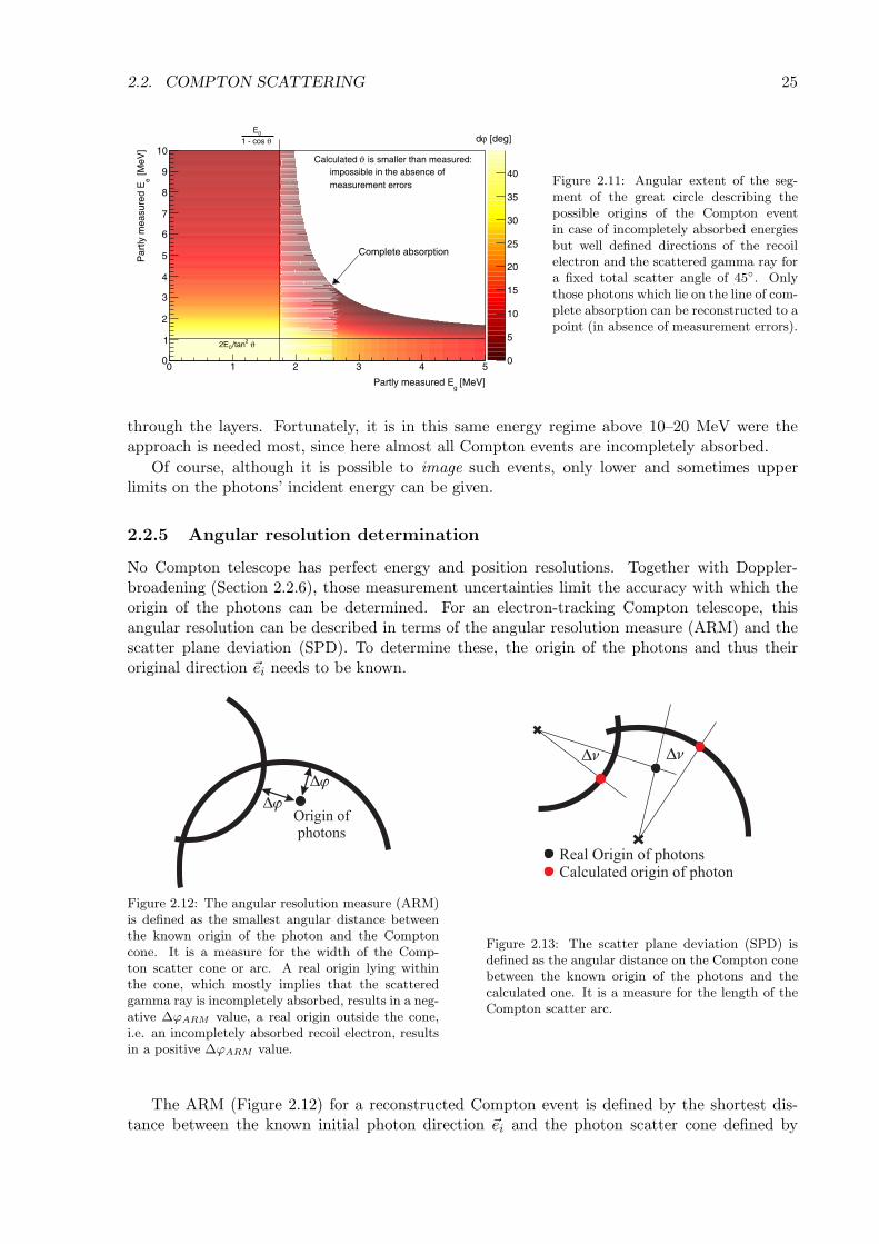
2.2. COMPTON SCATTERING 25
[MeV]g
Partly measured E
0 1 2 3 4 5
[MeV
]e
Par
tly m
easu
red
E
0
1
2
3
4
5
6
7
8
9
10
0
5
10
15
20
25
30
35
40
is smaller than measured:ϑCalculated impossible in the absence ofmeasurement errors
Complete absorption
[deg]ϕd ϑ1 - cos 0E
ϑ 2/tan02E
Figure 2.11: Angular extent of the seg-ment of the great circle describing thepossible origins of the Compton eventin case of incompletely absorbed energiesbut well defined directions of the recoilelectron and the scattered gamma ray fora fixed total scatter angle of 45◦. Onlythose photons which lie on the line of com-plete absorption can be reconstructed to apoint (in absence of measurement errors).
through the layers. Fortunately, it is in this same energy regime above 10–20 MeV were theapproach is needed most, since here almost all Compton events are incompletely absorbed.
Of course, although it is possible to image such events, only lower and sometimes upperlimits on the photons’ incident energy can be given.
2.2.5 Angular resolution determination
No Compton telescope has perfect energy and position resolutions. Together with Doppler-broadening (Section 2.2.6), those measurement uncertainties limit the accuracy with which theorigin of the photons can be determined. For an electron-tracking Compton telescope, thisangular resolution can be described in terms of the angular resolution measure (ARM) and thescatter plane deviation (SPD). To determine these, the origin of the photons and thus theiroriginal direction ei needs to be known.
Origin ofphotons
��
��
Real Origin of photonsCalculated origin of photon
�� ��
Figure 2.12: The angular resolution measure (ARM)is defined as the smallest angular distance betweenthe known origin of the photon and the Comptoncone. It is a measure for the width of the Comp-ton scatter cone or arc. A real origin lying withinthe cone, which mostly implies that the scatteredgamma ray is incompletely absorbed, results in a neg-ative ΔϕARM value, a real origin outside the cone,i.e. an incompletely absorbed recoil electron, resultsin a positive ΔϕARM value.
Figure 2.13: The scatter plane deviation (SPD) isdefined as the angular distance on the Compton conebetween the known origin of the photons and thecalculated one. It is a measure for the length of theCompton scatter arc.
The ARM (Figure 2.12) for a reconstructed Compton event is defined by the shortest dis-tance between the known initial photon direction ei and the photon scatter cone defined by

26 CHAPTER 2. INTERACTION PROCESSES
the (measured) direction of the scattered gamma ray. This shortest distance is equal to thedifference between the Compton scatter angle ϕ as calculated from the measured energies (ϕ bykinematics) and the angle between the known direction of the initial and measured direction ofthe scattered gamma ray (ϕ by scatter geometry):
ΔϕARM = arccos ( ei ◦ eg) − ϕ (2.20)
In the case of an incompletely absorbed recoil electron, the ARM is shifted to positive ΔϕARM ;in the case of an incompletely absorbed scattered gamma ray, the ARM is shifted to negativevalues.
The distribution of ARM values obtained from a larger sample of Compton events providesa measure of the directional accuracy of the Compton reconstruction. Conversely, the width ofthe ARM distribution therefore describes the uncertainty in the opening angle of the Comptoncone for each individual reconstructed Compton event.
From Figure 2.5, the analogy between electron and photon scatter cone is evident. Thus onecan also define an “Electron-ARM” in analogy to the “Photon-ARM”:
ΔεARM = arccos ( ei ◦ ee) − ε (2.21)
However, for the ultimate aim of Compton imaging, it is preferable to define the measurementaccuracies of the photon’s origin arising from both electron and gamma-ray scatter directionsrelative to the center of the photon cone — for the electron’s contribution this is done via theSPD illustrated in Figure 2.13. The SPD describes the angle between the true scatter planedescribed by ei and eg and the measured one spanned by eg and ee assuming that eg has beenmeasured correctly:
ΔνSPD = arccos (( eg × ei) ◦ ( eg × ee)) (2.22)
The SPD is relevant only if a measure of ee exists. It is dominated by the accuracy withwhich the direction of the recoil electron can be measured and provides a measure for the lengthof the Compton scatter arc.
In the case of MEGA, for all but the highest energies the ARM is the key parameter todescribe the angular resolution for a collection of Compton events, because the direction of thescattered gamma ray can be determined more accurately than that of the electron.
The ARM is influenced by most components of the measurement process, the accuracy ofthe energy of the electron and the scattered gamma ray as well as the accuracy with which thedirections can be determined. The energy resolution determines ϕ in Equation 2.20, the quantityarccos ‖ ei ◦ eg‖ is influenced by the position resolution. The propagation of measurement errorsfor the Compton scatter angle ϕ (Equation 2.6) leads to the following equation:
dϕ =E0
sin ϕ
√√√√( 1E2
g
− 1(Ee + Eg)
2
)2
dE2g +
1(Ee + Eg)
4 dE2e (2.23)
Figures 2.14 and 2.15 illustrate the dependency of this uncertainty on the measurement accuracyof the electron’s and the scattered photon’s energy, each time as a function of Compton scatterangle.
Especially from Figure 2.15 it is obvious that a Compton telescope which intends to measurelarge Compton scatter angles needs to measure the energy of the scattered gamma ray to a veryhigh precision to preserve its angular resolution.

2.2. COMPTON SCATTERING 27
Compton scatter angle [degree]0 20 40 60 80 100 120 140 160 180
[deg
ree]
ϕd
0
1
2
3
4
510% error
8% error
6% error
4% error
2% error
10% error
8% error
6% error
4% error
2% error
10% error
8% error
6% error
4% error
2% error
10% error
8% error
6% error
4% error
2% error
10% error
8% error
6% error
4% error
2% error
50 keV error
40 keV error
30 keV error
20 keV error
10 keV error
50 keV error
40 keV error
30 keV error
20 keV error
10 keV error
50 keV error
40 keV error
30 keV error
20 keV error
10 keV error
50 keV error
40 keV error
30 keV error
20 keV error
10 keV error
50 keV error
40 keV error
30 keV error
20 keV error
10 keV error
Compton scatter angle [degree]0 20 40 60 80 100 120 140 160 180
[deg
ree]
ϕd
0
5
10
15
20
10% error
8% error
6% error
4% error
2% error
10% error
8% error
6% error
4% error
2% error
10% error
8% error
6% error
4% error
2% error
10% error
8% error
6% error
4% error
2% error
10% error
8% error
6% error
4% error
2% error
50 keV error
40 keV error
30 keV error
20 keV error
10 keV error
50 keV error
40 keV error
30 keV error
20 keV error
10 keV error
50 keV error
40 keV error
30 keV error
20 keV error
10 keV error
50 keV error
40 keV error
30 keV error
20 keV error
10 keV error
50 keV error
40 keV error
30 keV error
20 keV error
10 keV error
Figure 2.14: Measurement uncertainty of the Comp-ton scatter angle dϕ as a function of the Comptonscatter angle ϕ. Only the measurement uncertaintyof the recoil electron is used. An initial energy of2 MeV was assumed. The solid lines correspond toan error in percent of Ee, the dotted lines to a con-stant error. The energy uncertainty of the MEGAprototype is a combination of both.
Figure 2.15: Measurement uncertainty of the Comp-ton scatter angle dϕ as a function of the Comptonscatter angle ϕ. Only the measurement uncertaintyof the scattered gamma ray is used. An initial energyof 2 MeV was assumed. The solid lines correspondto an error in percent of Eg, the dotted lines to aconstant error.
2.2.6 Doppler broadening as a lower limit to the angular resolution of aCompton telescope
In a real-life detector system the electrons are neither free nor at rest, but bound to a nucleus.In 1929 DuMond (1929) interpreted a measured broadening of Compton spectra as Dopplerbroadening induced by the velocity of the electrons. To describe this effect, a more sophisticatedCompton cross section than the Klein-Nishina equation is required: the momentum distributionof the bound electrons must now be taken into account. A suitable expression has been derivedby Ribberfors (1975) and called bound Compton cross section
(dσ
dΩ
)C, bound, i
=(
dσ
dΩ
)C, unbound
SIi (Ei, ϕ, Z) (2.24)
The SIi is called the incoherent scattering function of the i-th shell electrons in the momentum
approximation; it has been calculated by Ribberfors and Berggren (1982). Z is the atomicnumber of the scattering material.
Figure 2.16: Compton cross section for bound andunbound Compton scattering in Silicon: While bothcurves are practically identical at energies above sev-eral 100 keV, for lower energies Compton scatteringon bound electrons has a slightly higher probabilitythan on unbound electrons.
Figure 2.17: Cross section for bound and unboundCompton scattering in Silicon as a function of theCompton scatter angle at 100 keV. Both areas arenormalized to 1 (arbitrary units, linear scale). In thebound case, small and large scatter angles are slightlysuppressed.

28 CHAPTER 2. INTERACTION PROCESSES
Compared with Compton scattering on free electrons at rest three consequences arise:
• The total scatter probabilities change (Figure 2.16). Especially at lower energies, photonshave a slightly higher probability to scatter than predicted by the Klein-Nishina equation(Equation 2.10) for unbound electrons.
• The scatter angle distribution changes (Figure 2.17): Compared to the Klein-Nishinaequation small and large scatter angles are slightly suppressed. This effect is smaller athigher energies.
• The energy distribution between recoil electron and scattered gamma ray changes, whilethe sum of the interaction energies is still exactly equal to the total gamma-ray energy.As a consequence, the measured scatter angle and the one calculated using the standardCompton equation 2.6 differ. For a given point source location, an ARM distribution ofthe calculated origins shows a broadening (see Figure 2.18). Therefore this effect is widelyknown as Doppler broadening.
Figure 2.18: Cumulative ARMprofile for Compton scattering of200 keV photons in Silicon with-out scatter angle selections (basedon simulations). The differentareas represent the contributionsof different shells of the Siliconatom: in the outside shells, theelectrons are less energetic andcloser to the “target-at-rest” as-sumption. Therefore the distri-bution is sharper. The effectsshown are due to Doppler broad-ening only — all energy and po-sition measurements are assumedperfect!
For a Compton telescope the first two points have little impact other than slightly modifyingthe event distributions and total sensitivity for lower energies. But since there is no way todetermine the initial momentum of the electron, the third point gives rise to a lower limit forthe angular resolution of Compton telescopes.
From the formulation of the incoherent Compton scatter function in Equation 2.24, it shouldbe obvious that the Doppler-limited angular resolution depends on three parameters: the initialphoton energy Ei, the Compton scatter angle ϕ and the atomic number Z.
An example for the shape of a Doppler-broadened ARM profile is shown in Figure 2.18.The total profile is composed of the profiles of the different shells: the innermost electrons (1sorbital) have the highest momentum, and therefore the widest distribution. The 2p orbital ispopulated by 6 electrons, whereas all other orbitals consist of two electrons. For this reason the2p orbital contributes most to the width of the profile. The outermost electrons have the lowestmomentum and therefore form the peak of the distribution.
Figure 2.19 shows the dependence of the angular resolution on the atomic number. Onaverage, the angular resolution worsens with increasing Z. But it also strongly depends on theshell structure of the individual atoms. Up to Calcium (Z=20) the relationship is simple: itincreases until it reaches a noble gas (He, Ne, Ar), then the FWHM decreases and reachesa minimum at the alkaline metals or alkaline earth metals. For higher atomic numbers thenoble gases Krypton, Xenon and Radon are only smaller local maxima. The three highest localmaxima around Z=30, Z=46 and Z=79 are reached when the 3d, 4d and 5d orbitals are filled

2.2. COMPTON SCATTERING 29
Figure 2.19: Dependence of the angular resolution on the nuclear charge. The best angular resolution is obtainedfor alkaline or alkaline earth metals. The worst FWHM is reached when orbitals are completely filled (e.g. fornoble gases).
Material Si Ge CdZnTe Xe NE213 CsI NaIFWHM at 200 keV [degree] 1.80 2.85 3.50 3.30 1.75 2.95 3.00FWHM at 500 keV [degree] 0.80 1.25 1.55 1.45 0.75 1.25 1.40FWHM at 1000 keV [degree] 0.40 0.65 0.85 0.80 0.40 0.75 0.85
Table 2.1: Doppler broadening in different semiconductor materials, Xenon, and scintillators.
for the first time. For example, 46Pd is the maximum, not 48Cd, because of its special electronconfiguration: the two electrons from the 5s orbital are filling the 4d orbital. Similar reasonscan be found for other extraordinary local maxima, e.g. for 24Cr the 3d orbital is half filled.
Of the Compton telescope materials currently under serious consideration, Silicon providesthe best angular resolution assuming ideal detector properties, followed by Germanium andfinally the noble gas Xenon. Table 2.1 summarizes the performance of different semiconductorand scintillator materials. Some hydrocarbon-based scintillators like NE213, which was used asthe scatter material in COMPTEL, have a slightly better performance than Silicon due to theirhydrogen component.
The angular resolution also strongly depends on the Compton scatter angle ϕ (see Figure2.20). The FWHM worsens with larger scatter angles and therefore with smaller energies of thescattered photon. Since Doppler broadening results in a slightly different energy distributionbetween scattered gamma ray and recoil electron than would be observed in a Compton scatteron a free electron, its effects are similar to the energy measurement errors illustrated in Figures2.14 and 2.15.
Figure 2.21 summarizes the relationship between the initial photon energy and the angularresolution: On average Silicon has a Doppler-broadening limit on the angular resolution roughly1.6 times better than that of Germanium and roughly 1.9 times than that of Xenon. All threecurves roughly follow a power law with α = −0.75.

30 CHAPTER 2. INTERACTION PROCESSES
Figure 2.20: Dependence of the angular resolution onthe Compton scatter angle ϕ for Germanium at fourenergies at the Doppler-broadening limit. All valuesare averaged within 10◦-bins.
Figure 2.21: Dependence of the angular resolution onthe energy of the initial gamma ray at the Doppler-broadening limit. The values are averaged in 200 keVintervals below 1100 keV and in 400 keV intervalsabove 1100 keV. No event selections were applied.
Doppler broadening constitutes a fundamental limit for the angular resolution of Comptonscattering-based telescopes. Unfortunately, it makes several strategies to improve Comptontelescopes at these energies futile:
Due to their superior stopping power, high Z materials (e.g. Ge, CdTe, Xe) are sometimesfavored in gamma-ray astronomy. They guarantee a high efficiency; however, the associatedangular resolution is fundamentally limited. In particular, Germanium Compton telescopescannot take advantage of their good energy resolution to improve their angular resolution. Theyhave already reached their Doppler limit (Boggs et al., 2000b) at lower energies.
From the Doppler-broadening point of view, a Compton telescope based on semiconductortechnology should use Silicon or Carbon detectors as scatterer since these promise the bestangular resolution. However, they need much more material to achieve the same efficiency, ande.g. the energy resolution of Silicon is worse than that of Germanium.
For tracking Compton telescopes like MEGA, the scatter angle dependence of the Dopplerbroadening seems to be a disadvantage. An electron needs a certain amount of energy topass through several layers of material, inducing a bias towards larger scatter angles for trackedevents. Consequently, tracked events will tend to correspond to events where the role of Dopplerbroadening is more pronounced. However, since a reasonable amount of tracking sets in atincoming gamma-ray energies around 1-2 MeV, since the MEGA tracker is based on Silicon,and since other measurement errors dominate, Doppler broadening is not the limiting factor inthe current implementation of MEGA.
Nevertheless, the wide tails of the Doppler-broadened ARM distributions constitute a sig-nificant problem. The events in those tails represent a background component for close sources,and thus make it more difficult to resolve sources in crowded fields, e.g. in the Galactic centerregion.
Doppler broadening is a fundamental limit for the angular resolution. Therefore belowroughly 1 MeV Compton telescopes cannot give a better angular resolution than coded masksystems like IBIS (Winkler et al., 2003) on board INTEGRAL, which has an angular resolutionof roughly 0.2◦. Even an ideal Silicon-based Compton telescope will not reach this value below1 − 2 MeV, with the exact angular resolution achievable depending on event selections.
2.3 Pair production
When the energy of the incoming gamma ray exceeds two times the rest mass of an electron,1.022 MeV, another interaction mechanism starts playing a role: the conversion of the gammaray to an electron-positron pair in the electromagnetic field of a nucleus. During this process

2.3. PAIR PRODUCTION 31
�e�p
Ei
En
EeEp
pe
pi
pn
pp�
Ei Energy of initial photonEe Energy of electronEp Energy of positronEn Energy transferred to nucleus/electronθe Electron scatter angleθp Positron scatter angleθ Opening angle pi Momentum of the initial photon pe Momentum of the electron pp Momentum of the positron pn Momentum of the nucleus/electron
Figure 2.22: Pair production and all notations: When the energy of the gamma ray exceeds 1.022 MeV, it can beconverted into an electron-positron pair. The positron later annihilates.
the photon gets completely absorbed and the nucleus takes over part of the photon momentum.This process is called pair production, pair creation, or gamma conversion and is described bythe following equations of energy and momentum conservation:
Ei = Ee + Ep + En + 2E0 (2.25)
pi = pe + pp + pn (2.26)
If the photon’s energy exceeds four times the rest mass of an electron, pair creation can alsohappen in the field of an electron. Here the momentum is not transferred to the nucleus, butinstead to the electron. While the recoil of the nucleus is converted to phonons and thus is notdetectable by conventional means, the recoil of the electron generates a track signature — intheory three tracks might be visible in the MEGA detector. The ratio of the probability for pairproduction on an electron to that for pair production on a nucleus is given by:
pelectron =1
CZpnucleus (2.27)
Here Z is the atomic number, which is 14 for Silicon, and C is a factor which depends on theincoming gamma-ray energy. At 100 MeV C = 1.2, at 6 MeV C = 2.6 (Evans, 1958). In theMEGA energy range the ratio of conversions on electron to the conversions on a nucleus is ≈1:30.
In all past and current gamma-ray telescopes the momentum transferred to the nucleuscannot be measured. Since the energy transfer is not very large (∼ 511 keV/c), an approximationof the original photon direction can be made by neglecting the nucleus’ recoil:
ei ≈ Ee ee + Ep ep
Ee + Ep(2.28)
In the case of the MEGA prototype, even the energy of electron and positron can in most casesnot be determined due to incomplete absorption. Thus an even more radical simplification isnecessary:
ei ≈ ee + ep (2.29)
Pair creation telescopes, like Compton telescopes, are limited in their angular resolution bythe interaction processes in a solid state detector. Ignoring instrument-specific uncertaintiessuch as position and energy measurement accuracy, two uncertainties remain: the unknown

32 CHAPTER 2. INTERACTION PROCESSES
recoil of the nucleus and the small-angle scattering (Moliere scattering) in the layers of thedetector. Figure 2.23 summarizes these fundamental limits for a MEGA-like tracker consistingof layers of 500 μm thick Silicon. The most probable momentum transfer to the nucleus is close
Energy [MeV]10 20 30 40 50 60 70 80 90 100
Energy [MeV]10 20 30 40 50 60 70 80 90 100
]°A
ngul
ar r
esol
utio
n lim
it es
timat
e [
0
2
4
6
8
10
12
14 Combined resolution limitMoliere resolution limit for one leptonRecoil resolution limit
Figure 2.23: The fundamental an-gular resolution limit for pairs isdetermined by the unknown re-coil of the nucleus and by theMoliere scattering of electron andpositron, while traversing throughthe initial layer. The impactof Moliere scattering depends onthe instrument’s geometry (layerthickness in the tracker, 500μmSilicon in this case). It is assumedthat the interaction occurs is thecenter of the layer.
to 0.511MeV/c, with the nucleus most likely moving away at 80◦ to 90◦ from the photon’sincident direction for photons of energies above 10 MeV (Modesitt and Koch, 1950). For Silicon,this results in an energy transfer of ∼5 eV which is 4 orders of magnitude below the detectionthreshold of MEGA. The angular resolution limit Δrecoil can be estimated to be:
Δrecoil ≈ arctanmec
2
Ei(2.30)
The Moliere scattering limit is given by Equation 2.1 for one electron. In calculating the limitshown in Figure 2.23 it was assumed that the pair production happens in the center of the layerand the incoming photon’s energy is shared evenly between electron and positron. The latterconstitutes a rough approximation; 20% to 80% of the incoming photon’s energy are transferredto the electron in the pair with about equal probabilities over the energy range of interest(see e.g. Evans, 1958). Consequently, the lower-energy particle’s direction might have a ratherlarge uncertainty, and the higher-energy particle a much smaller one. However, the combinedresolution limit shown in Figure 2.23 — which is based on this assumption of equipartition ofenergy — turns out to be only 20% lower than the angular resolution obtained in full-fledgedMonte Carlo simulations of the MEGA telescope (including energy and position uncertainties) inthe energy range below 20 MeV where Moliere scattering dominates the instrument’s properties.A more detailed description for MEGA including all uncertainties is given in Schopper (2001).

Part II
New analysis techniques for the nextgeneration of Compton and pair
telescopes
33

34
Chapter 3
Simulation and data analysisoverview
The next generation of tracking Compton and pair telescopes records significantly more informa-tion about the individual interactions of all particles involved than its predecessors COMPTELand EGRET. This additional information has to be used in a completely different way to deter-mine the sequence of the hits as well as the quality of the reconstruction. Since no time-of-flightinformation is available, mainly the kinematics and topology of the Compton interactions andof the electron and positron tracks can be used. In this context a completely new set of toolsfor data reduction and analysis had to be developed for this work. This toolset is bundled intoMEGAlib — the Medium Energy Gamma-ray Astronomy library.
The MEGAlib software package encompasses the complete data analysis chain, which con-sists of four basic steps: (1) data acquisition, either by measurements with the real detector orvia simulation, (2) calibration of real data or the introduction of measurement uncertainties tothe simulations respectively, (3) event reconstruction and (4) high-level data-analysis includingimage reconstruction, polarization analysis, sensitivity calculation, etc. For all those steps dif-ferent routines exist in MEGAlib. A schematic overview of the general data flow is shown inFigure 3.1.
This introductory chapter describes each of the four steps discussed above that are necessaryto go from raw measurements or simulations to the lowest-level common data representations,hits in energy and position, and on to high-level data end products. In the following chaptersthe high-level processing steps, the event and image reconstruction, will be discussed in muchgreater detail as these comprise the heart of this work.
3.1 From detector measurements to hits
The data acquired by the read-out electronics of MEGA is expressed in detector units. Theseunits are the ID numbers of the detectors and channels which have triggered and the output of theanalog-digital-converters in ADUs (analog-to-digital converter units). Additional informationavailable includes time of the trigger, the time gap between the first trigger in the tracker andthe first trigger in the calorimeter, the trigger pattern, and more. All this data is acquired bythe MEGAlyze program as seen in Figure 3.1. A detailed description of this program can befound in Schopper (2001).
The energy information of each channel is calibrated separately. The detector-specific in-formation is converted into physical units: ADUs are transformed into energies and channelnumbers into positions. In the case of a strip detector all signals of the x- and y-strips ofone detector have to be combined into interaction positions. In the case of depth-sensitive
35
36 CHAPTER 3. SIMULATION AND DATA ANALYSIS OVERVIEW
calorimeters the signal of both diodes is not only converted into energy but also into a depthmeasurement. After this step one event is represented by hits, each of which consists of energyand position in the detectors world coordinate system. An extensive overview of the single-hitcalibration methods can be found in Andritschke (2006). Those hits are the input for the laterevent reconstruction.
3.2 From simulations to hits
The main purpose of Monte-Carlo simulations is to accurately predict the measurements and ul-timately the performance of the detector — both on ground and in space. In the energy range ofthe MEGA telescope (from a few keV up to hundreds of MeV), the Geant Monte-Carlo softwarepackages are widely used. For each of those packages exist simulation interface tools in ME-GAlib. The workhorse is Geant3 (CERN: Application Software Group and Networks Division,1993) with its MGGPOD extension (Weidenspointner et al., 2005) for the simulation of orbitalbackground environments. Geant3 is well tested in the MEGA energy regime and has givenremarkable agreement between simulation and measurements of real satellites (Weidenspoint-ner et al., 2005). The object-oriented approach of Geant4 (Agostinelli et al., 2003) makes theprogram more adaptable to the users’ needs, and will in the future replace Geant3. Currentlyhowever, it is still in a rapid development phase, which turned out to make it less reliable thanGeant3.
The foundation for a realistic simulation of a telescope is laid long before the simulationitself. First, one has to ensure that the simulation program contains all physical processesrelevant for the telescope and the energy range. Especially the effect of Doppler broadening,which fundamentally limits the angular resolution of a telescope whenever it relies on Comptonscattering, is not included in the default Geant packages. The GLECS extension package byKippen (2004) addresses this problem for Geant3 and Geant4. Another important point is arealistic geometry description. In the Compton regime it is especially hard to stop the initialphoton completely, because the result of Compton scattering still remains a photon, ready forthe next Compton interaction, until it gets photo absorbed. Thus it is really important toinclude absolutely all passive materials at the right places, to allow for interactions in passivematerials. This will result in incomplete absorptions, activations from protons and neutrons ina space environment, and thus the generation of secondary particles in passive material as seenin real detectors. In addition the correct isotopic composition of all materials and correspondingcross-sections for all particle types to be encountered must be implemented. Only if both,detector mass model and physics implementation in the Monte-Carlo code are realistic enough,the resulting detector performance parameters will truly reflect what a real detector would see.
When the simulation is performed, the output information is already in energies and po-sitions, but highly idealized. Energy and position resolutions are perfect, no thresholds havebeen applied, etc. Ideally the correct measurement uncertainties should be introduced into thesimulated data such that analyzing measurements and corresponding simulations gives the sameresults. This step relies on more detailed detector characteristics than are used in the simulationand are summarized as “simulation interface” in the overview diagram of Figure 3.1. For eachsingle interaction in the detector, the simulation yields the exact amount of deposited energyand the exact interaction position. In real detectors, however, the position knowledge is noisy orrestricted to voxels (e.g. strips in Silicon strip detectors and crystals in the CsI calorimeters) andthe energy is noised by effects such as light yield, noise of read-out channels, etc. The “simula-tion interface” accounts for this by centering the positions in the individual voxel and applyinga Gaussian noise to the energy measurement and the depth resolution of the 3D calorimetersaccording to the width of the expected/measured distributions.
No detector is perfect, but has a certain amount of not working pixels (dead, not connected,

3.3. EVENT RECONSTRUCTION AND RESPONSE GENERATION 37
deactivated, etc.). These pixels introduce additional dead material, which has to be accountedfor. Thus, a certain percentage of all hits is rejected on a random basis.
Since a Compton telescope is a coincidence detector, at least two signals (for MEGA onefrom the tracker and one from the calorimeter), with a certain energy deposit (in the MEGAcase measured as a voltage) are needed to trigger the read-out of the detector. This minimumenergy deposit is called the trigger threshold. Since the threshold is constant neither in time norfor different channels in a real-life system, it is not implemented as a fixed energy but with aGaussian width, which is determined by the expected/measured trigger threshold distributions.If a simulated event does not fulfill the trigger criteria, it is rejected.
After a coincident event has triggered the read out, all channels are analyzed to determinewhether the energy deposit is more than 5 σ above the average noise-level of this channel. Alldeposits below this noise threshold are rejected. Normally this noise threshold is smaller thanthe trigger threshold and is therefore important to detect additional small-energy hits besidethe triggers. The noise threshold is implemented like the trigger threshold. However, of coursethe individual hit is only rejected if it lies below the noise threshold.
Each Compton detector has a coincidence window, during which it accepts events fromthe two detector systems. If during this time span another event interacts in the detector, arandom coincidence occurs. Applying coincidence windows as well as readout and reset times isnecessary to determine the dead time of the detector. Random coincidences constitute a sourceof additional background, especially in high-rate environments. The latter is not an issue forthe MEGA measurements analyzed in this work, since they were all taken in the laboratory.
After the steps discussed in this and the preceeding section, the real and the simulateddata should look very similar. The events are now represented by hits consisting of energy andposition.
3.3 Event reconstruction and response generation
During the next step, the individual hits must be combined into events (Revan library in Figure3.1) and the detector response matrices (Response generator in Figure 3.1) must be determined.
The methods of the event reconstruction are described in detail in Chapter 4. The basicidea is to look at the structure of the event, and from the kinematics, the topology and thedetector geometry along the lines-of-travel of the photons, electrons or positrons, find out whathappened in the detector: Did a Compton scattering occur or a pair creation, did a chargedparticle pass through or was a large shower created? At the end of the event reconstruction,the data is represented by event types and their associated information, e.g. a Compton eventwith given energy and direction of the recoil electron and the scattered gamma-ray, or a pairevent with given direction and energy of electron and positron. All events are accompaniedby a quality factor, which describes the probability that the event happened this way and iscompletely absorbed.
The second important task on this level of data analysis is to generate response matrices. Aresponse maps the properties of the incoming photons to the detector measurement in a multi-dimensional data space. In order to determine the response, the information of the incidencephotons from the simulation is compared with the characteristics of the reconstructed events.Since this data space is rather complex, different projections are made and optimized for specialtasks, for example finding the correct interaction sequence (event reconstruction response seeChapter 4) or determining the origin of a photon in image space (imaging response see Chapter5).
The result of this step of data analysis are events, and the description of how the detectorreacts on well defined inputs, the response. The next step is to use this information to retrievethe parameters of the original source distributions.

38 CHAPTER 3. SIMULATION AND DATA ANALYSIS OVERVIEW
3.4 High level data analysis
The last step, the high level data-analysis, tries to invert the measurement process and todetermine the properties of the sources of the measured gamma rays.
The first crucial step is to find optimized selection criteria for “good” events. The main taskof event selections is to exclude those bins of the data space that contain most of the backgroundevents. The high-level data analysis tools comprised in MEGAlib’s Mimrec library allow eventselection on basically all performance-relevant parameters of the Compton and Pair events.These include event type, start detector, energy, scatter angles, distance between interactions,event quality factors, earth horizon cut, number of hits, opening angle and initial deposit of thepair events, and many more.
Diagnostics tools assessing angular resolutions (ARM, SPD), energy dispersion, scatter angle(ϕ, ε, ϑ) distributions, etc. are necessary to determine the quality of the event selections as wellas the performance of the detector. Moreover, it is possible to perform background correctedpolarization studies, determine the effective area and sensitivity of a detector, and many more.
The most challenging step, however, is the image reconstruction itself, which is explained inChapter 5. The list-mode likelihood image reconstruction algorithm allows to reconstruct sourcesin spherical as well as Cartesian coordinates (2D as well as 3D) from tracked and not trackedCompton as well as pair events and allows several different levels of response approximations tobe applied to the data.
3.5 The scope of MEGAlib
MEGAlib is completely written in C++ and based on ROOT (Brun and Rademakers, 1997).It has accumulated over 300,000 lines of source code, most of which where written within thecontext of this work. Each result presented in this work has been achieved by using the MEGAlibsoftware package. The software is designed to be easily adaptable to different detector designs,from tracking Compton and Pair telescopes, via time-of-flight based Compton telescopes toDrift chamber based Compton telescopes. The necessary changes are restricted to defining anew geometry and detector description.
The MEGAlib package has been considered the most versatile and state-of-the-art tool setavailable in 2004 by the ACT study team. Consequently it has been used for different Comptontelescopes designs for the NASA Advanced Compton Telescope concept study (Boggs et al.,2005).
The next two chapters are dedicated to the two most challenging tasks in the data analysis oftracking Compton and pair telescopes, the event reconstruction and the image reconstruction.

3.5. THE SCOPE OF MEGALIB 39
������������������������ ������������������������
�� ���������!�� ���������!
����������
���� ������ �������
"#�����$�%��#����� &�����#�"#�����$�%��#����� &�����#�
�#$�#'���# #�������� �(�#$�#'���# #�������� �(
��#�)��#�) ���*+,���*+,��#�-��#�-
.�����/�� ���/�
$������&���#�/����
�'#���01� ���#/�
����/� &�#/����2
3����0#��!�
�#$��������#2
1��##����#$�
�,1���&#��
�� ���������!(�3����� ���������!(�3���44�'��$�����#��!����'��$�����#��!���
�����!5�����!5
���� ��� �������
�� ���������
.� &�����#��#�����.� &�����#��#�����
���������������������
������������������������
������������� ��
6���#���#�����6���#���#�����
�������������������
������������ ������ ���
�������������������
�������� ������!�����
������ ������ ����
1�#'��1�#'��44
���*+,���*+,
��������
"���
�����#
1��� �1��� �
"���
�����$
�1 �����(�1 �����(
%�&����������
��!���������
6'�#�������!(��'#�����#���&����#6'�#�������!(��'#�����#���&����#
' (!������� ����������������� �)����!�������������������
���������� ����* ����
' +���)������,������������� ������ ������������ �������
������� ����������-��#���� ����������������������� � ������
���� ������������������ �������!����
' ����������������� �������������������������������
������������ ��������������&��������� ��
' .������� �������������!����� ������ �������������
' ,������ ���� ��������/����������
' "������!�����& ,������ � �����������
' 0���������
' ����/��������!��������
' 1����!������������� �������
�������� ���������� ��
' 2���������!���
.�'�#�������!.�'�#�������!
3���*����/�
���������
����������
1���������#1���������#
4�����������
���� �������
�������������
3��$���(�3��$���(�
�����$����������$�����
Figure 3.1: Basic layout of the MEGAlib software package. See the text for a detailed description.

40 CHAPTER 3. SIMULATION AND DATA ANALYSIS OVERVIEW

Chapter 4
Event reconstruction
4.1 The basic idea
Valid events can generate a large number of different possible hit patterns in a combined Comp-ton and pair telescope such as MEGA. The greatest challenge on the path from the hits makingup a raw event to scientific results is figuring out what actually happened in the detector for eachindividual event. This process is called event reconstruction. Figure 4.1 illustrates a fraction ofthe variety of valid photon events, with lines illustrating the true sequence of event components.All shown events have been actually measured with the MEGA prototype.
While the following discussion is for the most part applicable to any modern-day Comptonor pair telescope, the discussion is geared towards, and the choice of data space dimensions isoptimized for, the MEGA instrument concept with its tracker consisting of thin Si layers.
4.1.1 Tasks and problems of the event reconstruction
The overall performance of a Compton and pair telescope is not only determined by its hard-ware but also by the performance of the algorithms which recover the original parameters of theincident photons from the measured data. Since each lost or not recognized event reduces theefficiency, and each incorrectly reconstructed event lowers the efficiency and increases the back-ground, the performance of the data analysis has considerable influence on the final sensitivityof the telescope.
Before the event reconstruction, an event consists of nothing but a collection hits which allhave position and energy information. The event reconstruction sorts those hits in the order inwhich the interactions of the original particle(s) inside the detector occurred. This is done byutilizing the laws of physics and statistical considerations. The result of this data analysis stepis an event which describes the main interaction which happened in the detector, for examplea Compton event with energy and direction of the scattered gamma-ray and recoil electron(including measurement errors), or a pair creation event with energy and direction of electronand positron. This information encompasses the parameters of the incident particle includingenergy and direction that are needed in the next step of data analysis.
Sequencing would be a trivial task if the hits had an accurate-enough time tag. But thecompact design of the MEGA instrument and the slow response of its detectors and read-outelectronics render this impossible. Thus the kinematics of the interactions, the topology of theevent structure, and the geometry of the detector have to be used to deduce the parameters ofthe original photon.
During the event reconstruction numerous questions emerge and have to be answered: Arethere tracks? Are there multiple tracks? Which hit belongs to which track? What endof the track is the starting point? Do all the other hits belong to the event? To which
41
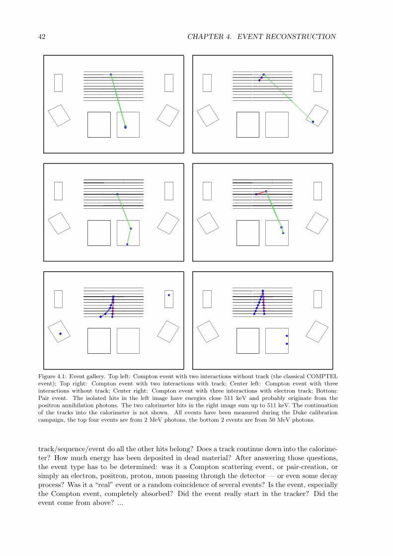
42 CHAPTER 4. EVENT RECONSTRUCTION
Figure 4.1: Event gallery. Top left: Compton event with two interactions without track (the classical COMPTELevent); Top right: Compton event with two interactions with track; Center left: Compton event with threeinteractions without track; Center right: Compton event with three interactions with electron track; Bottom:Pair event. The isolated hits in the left image have energies close 511 keV and probably originate from thepositron annihilation photons. The two calorimeter hits in the right image sum up to 511 keV. The continuationof the tracks into the calorimeter is not shown. All events have been measured during the Duke calibrationcampaign, the top four events are from 2 MeV photons, the bottom 2 events are from 50 MeV photons.
track/sequence/event do all the other hits belong? Does a track continue down into the calorime-ter? How much energy has been deposited in dead material? After answering those questions,the event type has to be determined: was it a Compton scattering event, or pair-creation, orsimply an electron, positron, proton, muon passing through the detector — or even some decayprocess? Was it a “real” event or a random coincidence of several events? Is the event, especiallythe Compton event, completely absorbed? Did the event really start in the tracker? Did theevent come from above? ...

4.1. THE BASIC IDEA 43
While answering those questions, the event reconstruction has to cope with missing andsurplus hits, which both significantly complicate things. The missing hits originate from inter-actions in passive material such as structure or dead voxels and from hits whose energy depositis below the threshold. The latter proves especially problematic for Compton events with trackswhere the electron did not deposit sufficient energy in the layer of the Compton interaction. Thisleads to missing energy as well as to a wrong start position of the track. Surplus hits are gen-erated by general detector noise and random coincidences. At higher energies, bremsstrahlungfrom decelerated electrons also plays a role. Finally, the poor energy and position resolution inthe calorimeters constitutes a definite handicap to determine the overall hit sequence of multipleCompton events.
4.1.2 Outline of the event reconstruction
The event reconstruction tries to identify the most simple structures like pair events and muonsfirst. The remaining event are searched for the much more complex structures of Comptonevents, to which most of this chapter is dedicated. The individual steps are outlined below.
Step 1: Clusterize hits in adjacent bars and stripsWhen an electron passes through a Silicon wafer it might hit two or more adjacent strips.Those adjacent hits are combined into a cluster of hits. The energy of the cluster is the totalenergy of its hits and its position is the “center of energy”. The detailed algorithm for themore complex case of several interactions in one Silicon wafer is described in Section 4.2. Undercertain circumstances (high electron energies, interactions close to the border) electrons are alsotraveling from one CsI bar to the next bar in the calorimeter. In this case the two hits arecombined into a cluster if the difference in depth position is not larger than 3 sigma of the bars’depth-position (“z”) resolution.
Step 2: Search for a vertex to identify pairsPair events produce a very characteristic pattern in the MEGA detector, an inverted “V”, whichcan be easily recognized not only by eye (see e.g. Figure 4.1) but also by a pattern recognitionalgorithm. If a vertex is found, the event is considered a pair event, and the correspondingreconstruction algorithm is applied (details see 4.3).
Step 3: Search for high energy charged particle eventsHigh energy charged particles such as muons also create easily recognizable structures in thetracker: One rather straight track per particle passing through the tracker. If one (or more) ofthose signatures are found, the high energy charged particle reconstruction algorithm is launched,which fits a straight line to the pattern in the detector. Such muon events have been used indetector testing and calibration. Since this algorithm is rather trivial no individual section isdedicated to it in the later text.
After step 3, all easily recognizable patterns have been found. The remaining events are Comptonevents or “trash”.
Step 4: Search for Compton electron tracksThe initial step in the focused search for good Compton events is the identification of anyelectron tracks and the determination their direction of motion. This is done by scrutinizing the

44 CHAPTER 4. EVENT RECONSTRUCTION
topology of the track and its kinematics, especially the energy deposits in the wafers and thechange in direction during the passage through one wafer (see 4.4).
Step 5: Search for the Compton interaction sequenceThis step aims to arrange all interactions (tracks are now one interaction with their start asposition of the interaction) in their kinematically correct order. Keys are the direction of theelectron track, and, if the event consists of three or more interactions, the available redundantinformation from the multiple Compton interactions, as well as the detector geometry, especiallyabsorption probabilities along the path of the photon (see 4.5).
Step 6: Search for special beta-decaysThe last step could be a search for characteristic signatures of beta-decays in the active materialof the detector. Activation is a significant background source for a real satellite mission. Betadecays have a signature which might be partly identified by certain types of Compton telescopes:One hit is generated by the β+ particle itself, other signatures by the released photons. In casesome sub structures (sub collection of hits) of the event have the same energies as the (well-known) photon(s) produced by the decay and another hit is within the possible flight directionof that photon, then that event could be rejected. However, an excellent energy (dE/E < 0.01)resolution is necessary for this to be feasible. Thus this approach is not explored for MEGA.
The resultAt the end of the event reconstruction process the events are described by their main interactionprocess: Compton, Pair, Muon, Shower, etc. Since it is not possible to uniquely reconstruct forexample Compton events to a unambiguous position on the sky — one always has the Comptoncone, an arc or a more complex structure, which is associated with the measurement uncertaintiesaccompanied by the interaction process — it is important to keep the information about themain interaction process and not only the final information about the incoming particle. Inaddition, a quality factor resulting from the underlying statistical approach of sequencing isassociated with each event. This quality factor can be used for event selections in the lateranalysis.
4.1.3 Approaches for complex reconstruction tasks
For all different event types one must sort and sequence hits, and decide on the best (i.e. mostlikely) order. The “rules” are provided by the underlying physics: the interaction of the electronswith the layers of the tracker, the kinematics of multiple Compton events, etc. However, forpairs and high energy charged particles this process is much easier: for pairs the start point caneasily be found, and e.g. muons are only straight lines in the tracker. The main work has to bedone for Compton events, to which the largest part of this chapter is dedicated.
While a number of different approaches have been investigated during the course of thiswork, those based on a real statistical quality factor, like correlations, χ2 statistics, Bayesianstatistics, etc., have proven to give the best performance for the general case of a trackingCompton and pair telescope and are the only ones discussed here. For each of the two mostchallenging reconstruction tasks (electron tracking and Compton sequence reconstruction) twomethods will be discussed: A simple analytic approach which only uses the most importantaspect of the data space, and a significantly more difficult approach based on a large data space,which uses as much information as can be retained.
The simple approach in both cases follows the following principles: It should be fast, thereshould be no extensive preparations necessary (e.g. calculation of response matrices) and it

4.2. CLUSTERIZING 45
should be largely independent of the geometry and the detectors’ energy and position resolution.For the electron tracking, this is done by correlations (Pearson, Spearman-Rank) which are basedon the fact that the angular deviation as well as the energy deposit per layer increase along thetrack. For the Compton sequence reconstruction, a simple χ2 test statistics is used. It exploitsthe redundant information available in the case of a track or of multiple Compton interactions.
The more complex approach in both cases is implemented via Bayesian statistics. Inter-actions of the particles in the detector are described by probability density functions in manydimensions, and, after applying Bayes’ theorem, one can calculate the probability of the foundsequence being correctly ordered. This approach traces much better what really happened inthe detector and can include all imperfections of the telescope, and thus will likely give bet-ter results. However, the underlying physics is described by many parameters, leading to amulti-dimensional probability density function. Taking into account the fine binning required todescribe the physics in adequate detail, in the case of MEGA this results in response matriceswith 108 bins and more. To obtain the necessary statistics, an average factor of ∼100 or moregood, i.e. fully absorbed events in the correct sequence, are needed per bin to fill the matrix.Performing the necessary simulations required roughly one CPU year of simulation time on a2.4 GHz Xeon CPU (of course a lot of CPUs were used).
As expected, the Bayesian methods result in a slightly better performance at the cost ofsignificantly increased CPU consumption.
In the following sections all non-trivial algorithms of the outline in Section 4.1.2 will bediscussed.
4.2 Clusterizing - multiple hit recognition in double-sided stripdetectors
Most of the semiconductor detectors which are currently being considered for Compton tele-scopes are strip detectors, with the strips running perpendicular to each other on the top andbottom side of a wafer. The position of the interaction has to be recovered by finding the inter-section of those strips which registered an energy deposit. Only after this step is completed thehits have positions which are needed for event reconstruction.
In the simple case of Compton events, where one traversing electron deposits energy in oneor more neighboring strips on both (n and p) sides of the layer, the single position can simplybe calculated via the energy-based center of gravity on both sides:
x (in, ip) =(∑
in inEni∑
in Eni
,
∑ip ipEp
i∑ip Ep
i
)(4.1)
where the sum is over all hit, neighboring strips ix in the cluster and Exi is the deposited energy
in strip ix.For pair events the task of clusterizing is somewhat more complex. If multiple charged
particles pass through one layer, the resulting position ambiguity cannot be resolved from theknowledge of the affected strips alone. Figure 4.2 illustrates an example of a pair creationin the field of an electron, which constitutes a worst case scenario: Two electrons and onepositron pass through one Silicon layer. In addition to the three true interactions, there are 6more intersection points of affected n and p strips that correspond to also-possible interactionsites. All 3 × 3 = 9 possible interaction sites are marked by an × in Figure 4.2. Thus 3! = 6permutations have to be considered: The strips (an, bn, cn) on the n-side can be combined withthe permutations (ap, bp, cp), (ap, cp, bp), (bp, ap, cp), (bp, cp, ap), (cp, ap, bp) and (cp, bp, ap) of p-side strips. The energies on n- and p-side for each individual hit are in best agreement for the

46 CHAPTER 4. EVENT RECONSTRUCTION
γ
recoil e+ −−ee Figure 4.2: The rare pair creation on anelectron produces three trackable parti-cles, one positron and two electrons. Inthe simplest case, on p- as well as on n-side of the Silicon layer three strips areintersected, leading to nine possible in-teraction positions.
correct permutation, which can be found using a generalized form of a χ2-statistics to compareall possible combinations:
QS =1N
N∑i,j=1
(En
i − Epj
)2
(σni )2 + (σp
j )2 ∀ permutations (4.2)
σi is the error of the energy measurement in strip i. The correct permutation is associated withthe smallest quality factor QS , since then the En and Ep are in agreement within measurementerrors.
For a real-life detector the algorithm has to cope with additional problems:
• In the case of the MEGA prototype a significant amount (typically 15%) of strips are dead.Thus it is likely that for one hit there will be a x-y-position but for the other only a x- oronly a y-position.
• If on one side two well separated strips are triggering and on the other side only one strip,but with significantly higher energy, then two electrons passed through one strip one thesecond side. Those hits need also be separated by the algorithm.
The algorithm recognizes the correct interaction locations for roughly 90% of pair eventsrecorded by the MEGA prototype. Unfortunately the expected energy deposit of an elec-tron/positron passing through one wafer does not strongly dependent on the electron’s energyand follows a fairly narrow Landau-distribution (see 2.1.2). Therefore it is likely that a similarenergy within the energy resolution of n and p strips of the wafer will be deposited at the differentinteraction sites and thus the wrong permutation might be chosen. Nevertheless, even the 90%identification rate for the prototype is high enough to identify the topology of the pair-inducedtracks. Thus the remaining wrongly identified interaction locations can be recovered during pairevent reconstruction (details see 4.3.1).
From now on no distinction is made anymore between “hit” and “cluster”. A “hit” mightalso consist of sub-hits in adjacent bars or strips, i.e. actually be a cluster.
4.3 Identifying and reconstructing pair events
Step 2 of the outline from Section 4.1.2 is the search for a vertex in the tracker to identifypairs. During gamma conversion an electron and a positron are created, the so called pair. Amore detailed description of the pair creation process can be found in Section 2.3. Starting

4.3. IDENTIFYING AND RECONSTRUCTING PAIR EVENTS 47
Figure 4.3: A worst case vertex which fulfills the min-imum requirements: It starts with a layer with onehit, in one of the preceeding (seven) layers at leasttwo have exactly two hits.
Figure 4.4: Illustration of the reconstruction of pairevents. For details see text.
from their creation point, the electron and positron move in different directions. This creates acharacteristic pattern in the MEGA tracker, an inverted “V”: In most cases there is only onehit in the layer of the interaction, but two hits in the successive layers. In the following such astructure is called a vertex. It is the main characteristic for identifying pair events.
4.3.1 Method
The pair reconstruction algorithm consists of three main steps: identify the vertex, append allother hits to the electron or positron track, and finally do some post processing.
Step 1: Find the vertexIn a real-life detector, a pair must be allowed to have several missing interactions, either becauseelectron and positron might have passed through dead material between the wafers or throughdead strips. In addition, there might be several additional bremsstrahlung hits. Thus thedefinition of the vertex needs to be very fault-tolerant:
• One layer contains exactly one hit (the starting point)
• In the n following layers below the starting point at least two layers contain exactly twohits
• There is no hit in m layers above the starting point
An example which exactly fulfills the minimum requirements of this vertex definition can befound in Figure 4.3. The first question to ask is how easy it is to find a continuation of thevertex. In algorithmic terms, this comprises checking each consecutive layer of the tracker (topto bottom, after a first initial interaction is found) if it contains exactly two hits. The number(n) of consecutive layers of the tracker containing a total of two layers with exactly two hits eachis a measure for track quality — the less layers have to be searched to find this pattern, the morereliably one can assume to be looking at a genuine vertex signature. In the case of MEGA, fora laboratory prototype in a strong beam no restriction on this parameter is necessary, while thesimulated satellite performed best with n constrained to no more than four consecutive layersin the presence of background. The other parameter is the number of layers (m) above the start

48 CHAPTER 4. EVENT RECONSTRUCTION
point which may not contain any hits. Since the probability that two interactions happen inthe whole tracker of the satellite geometry is on average 15%, this parameter is not critical andthus set to two.
Step 2: Append all hitsIf a vertex is found (i.e. all 3 conditions above are fulfilled with a suitable n and m), then bydefinition the start position of the pair is known. Starting from this initial interaction position,the initially assumed directions of the electron and positron track are the directions to the hitsin the first layer with two hits.
After the initial directions of the tracks are determined, each consecutive layer is searchedfor a continuation of the tracks. Whenever multiple combinations of measured hits into tracksare possible, the alternative resulting in the straightest tracks is chosen. “Straightest” here isdefined as the assignment of hits to tracks, for which the following quality factor is smallest:
QD = Δθ2e,i + Δθ2
p,j (4.3)
where Δθe,i is the direction change of the electron track, if the track is connected to the ith hitin the next layer; similar for Δθp,j.
The reconstruction accounts for missing hits as well as additional bremsstrahlung hits. Thelatter can result in more than two hits in one layer, or in a hit not consistent with eithertrack. Whenever the energy of a hit is below the minimum energy deposit to be expected fromthe vertex electron or positron according to the Landau distribution, this hit is flagged as abremsstrahlung hit and ignored in the search for the straightest vertices. After all tracks arefound, the energy of all additional hits is added to the closest track’s energy. This includes hitsfrom the calorimeter. The energy of the first interaction, as well as the energy of hits after thestarting point which are consistent with both tracks, is evenly distributed between the electronand positron.
Step 3: Post-processingAlthough a vertex is a clear indication for a pair event, some of the tracks need post-processing.Sometimes the strip ambiguity discussed in Section 4.2 had not been correctly resolved, resultingin wrong intersection points. As consequence the tracks appear curved instead of straight (seeFigure 4.5 for an example). To solve this problem, for each track a quality factor is calculatedbased either on a Pearson-correlation or on Bayesian statistics. The quality factors describeshow good the tracks conforms with the expected physics. They are discussed in more detail inthe context of Compton electron tracking in Sections 4.4.2.2 and 4.4.2.3. For the layer underinvestigation (3 in Figure 4.5), they are calculated without the hits of this layer but layer 2 and4 directly connected — once in the given order, and once when the tracks below this layer areexchanged. If the quality factors for the exchanged tracks is better, this new direction is chosenas the correct one. The hit positions in layer 3 are ignored in this case and their energies areadded in equal parts to the two tracks.
As a final step, one could in principle attempt to correct the measured energy by determin-ing the incident photon’s energy from the vertex opening angle as well as the change of theenergy deposit and scatter angle along the tracks. The feasibility of such approaches has beendemonstrated by e.g. Fichtel et al. (1975) for spark-chamber systems and higher-energy pairs.The same approach should be applicable to MEGA.

4.3. IDENTIFYING AND RECONSTRUCTING PAIR EVENTS 49
12
2
3
3
3
4
4
3
5
5
6
6
Figure 4.5: Illustration of the consequencesof wrong interaction mapping during theclusterizing process. The figure shows atop view of the track, the numbers indi-cate the layer of interaction. In layer 3the interaction mapping (see Section 4.2)is wrong. The white circles in layer 3represent the correct interaction positions,the black ones are the wrongly mappedones. As consequence the path of elec-trons/positrons is wrong: the black path isthe wrongly reconstructed path, the greypath is the correct one. This problem isresolved during post-processing (details seetext).
4.3.2 Performance
Figure 4.6 illustrates the direction-reconstruction performance of the pair tracking algorithm for20 MeV photons (on-axis incidence, MEGA Satellite geometry). Considering only events whichfulfill the requirements for an initial identification as pair event set forth in the previous section,the distribution of the deviation of the reconstructed from the true direction of incidence isshown.
Overall, it is evident that the vast majority of events is reconstructed correctly to withinsignificantly better than 10◦. 68% of directions are reconstructed to better than 5.75◦ which ismainly limited by Moliere scattering. At small deviation angles, a smaller absolute number ofevents per angular bin are recorded. This is a purely geometrical effect — if counts/sr were showninstead, the distribution would continue to rise monotone towards smaller deviation angles.
For most events that appear at large direction deviations, the core of the pair recognitionalgorithm still worked. Multiple effects contribute to such large deviations; for the most partthese could only be overcome in a different instrument geometry:
• If the energy of electron and/or positron are not measured correctly (due mostly to leakagefrom the instrument, sometimes due to wrong reconstruction of the later electron/positronpath), applying Equation 2.28 will yield a wrong origin direction. This is especially pro-nounced for large opening angles. A larger instrument with thicker calorimeters wouldperform better in this respect.
• Strong Moliere scattering within the layer of pair creation renders an accurate measurementof the electron’s direction impossible. Thinner layers in the tracker could significantlyreduce this effect.
• Especially for close tracks of electron and positron, the limited spatial resolution of thetracker limits the accuracy to which the incident direction can be reconstructed. Clus-terization potentially compounds this problem — but the benefits of this approach faroutweigh the disadvantage that comes to light in this particular case. A much finer strippitch of the tracker would contribute to a better overall angular resolution especially forhigher-energy pair events.
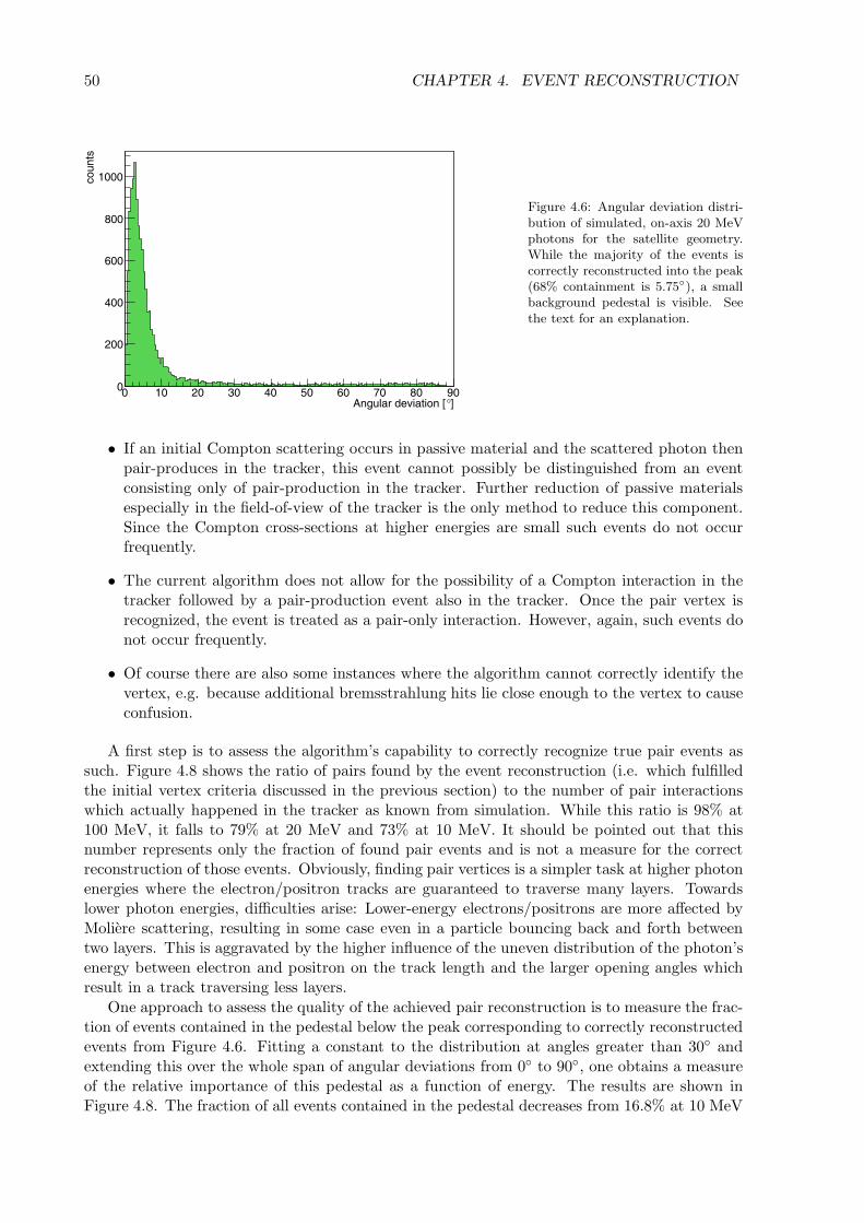
50 CHAPTER 4. EVENT RECONSTRUCTION
]°Angular deviation [0 10 20 30 40 50 60 70 80 90
coun
ts
0
200
400
600
800
1000
Figure 4.6: Angular deviation distri-bution of simulated, on-axis 20 MeVphotons for the satellite geometry.While the majority of the events iscorrectly reconstructed into the peak(68% containment is 5.75◦), a smallbackground pedestal is visible. Seethe text for an explanation.
• If an initial Compton scattering occurs in passive material and the scattered photon thenpair-produces in the tracker, this event cannot possibly be distinguished from an eventconsisting only of pair-production in the tracker. Further reduction of passive materialsespecially in the field-of-view of the tracker is the only method to reduce this component.Since the Compton cross-sections at higher energies are small such events do not occurfrequently.
• The current algorithm does not allow for the possibility of a Compton interaction in thetracker followed by a pair-production event also in the tracker. Once the pair vertex isrecognized, the event is treated as a pair-only interaction. However, again, such events donot occur frequently.
• Of course there are also some instances where the algorithm cannot correctly identify thevertex, e.g. because additional bremsstrahlung hits lie close enough to the vertex to causeconfusion.
A first step is to assess the algorithm’s capability to correctly recognize true pair events assuch. Figure 4.8 shows the ratio of pairs found by the event reconstruction (i.e. which fulfilledthe initial vertex criteria discussed in the previous section) to the number of pair interactionswhich actually happened in the tracker as known from simulation. While this ratio is 98% at100 MeV, it falls to 79% at 20 MeV and 73% at 10 MeV. It should be pointed out that thisnumber represents only the fraction of found pair events and is not a measure for the correctreconstruction of those events. Obviously, finding pair vertices is a simpler task at higher photonenergies where the electron/positron tracks are guaranteed to traverse many layers. Towardslower photon energies, difficulties arise: Lower-energy electrons/positrons are more affected byMoliere scattering, resulting in some case even in a particle bouncing back and forth betweentwo layers. This is aggravated by the higher influence of the uneven distribution of the photon’senergy between electron and positron on the track length and the larger opening angles whichresult in a track traversing less layers.
One approach to assess the quality of the achieved pair reconstruction is to measure the frac-tion of events contained in the pedestal below the peak corresponding to correctly reconstructedevents from Figure 4.6. Fitting a constant to the distribution at angles greater than 30◦ andextending this over the whole span of angular deviations from 0◦ to 90◦, one obtains a measureof the relative importance of this pedestal as a function of energy. The results are shown inFigure 4.8. The fraction of all events contained in the pedestal decreases from 16.8% at 10 MeV

4.4. COMPTON ELECTRON TRACKING 51
5�55
5�-5
5�$5
5�65
5�75
8�55
8�-5
5 -5 $5 65 75 855 8-5
�#��!�7�8
9������#��������#�5$������
'#��
5�5
-�5
$�5
6�5
7�5
85�5
8-�5
8$�5
86�5
87�5
5 -5 $5 65 75 855 8-5
�#��!�7�8
1�#����&���#�����������&#$�
�$�����7:8
Figure 4.7: Fraction of pair events recognized as such.The true amount of pair creations in the tracker isknown from simulations. The higher the energy, theeasier the vertex signature can be found in the tracker.This number only describes how many pair events wererecognized; no conclusions can be drawn about theaccuracy of their reconstruction.
Figure 4.8: Contribution of the background pedestalfrom the angular deviation distribution (see Figure4.6) the total number of identified pair events. Thehigher the energy of the incident photon the simpleris the reconstruction, the less likely large angular de-viations appear. See the text for an explanation of allthe reasons.
to 9.5% at 20 MeV and 1.5% at 100 MeV.Besides the argumentation above, at lower energies the number of wrongly reconstructed
events increases due to Compton tracks which are identified as vertices, when their tracks havesharp reverse points, i.e. switch from moving bottom-top to top-bottom. However, for on-axis incidence this happens mostly in cases, when the first interaction was not in the tracker,because Compton kinematics only allows for a maximum recoil electron angle of 90◦ (Equation2.8). Finally most of the wrong reconstructions have larger opening angles. Only allowing anopening angle of 45◦ of 10 MeV pairs reduces the pedestal by a factor of 2 while reducing theoverall number of detected pairs by only 22%. This will be one of the key event selections forbackground rejections for the final satellite simulation in Chapter 10.
4.4 Compton electron tracking
For the electron and positron tracks making up a pair event, the direction of motion is welldefined by the vertex. For Compton electrons, finding the direction of motion is a much moredifficult process which has to use the complete kinematics of the track.
4.4.1 The data space of electron tracking
An electron deposits its energy mainly via ionization and bremsstrahlung, and the deviation ofits path through matter from a straight line is due to Moliere scattering (see Chapter 2.1).
The underlying physics of the interaction process of electrons with matter determines theproperties of a real electron track. They can be used to determine the direction of motion ofthe electron for a given measured track. These general properties of an electron track are:
1. The angular deviation Δα from layer to layer of the track increases according to Molierescattering.
2. The energy deposit Edep in the wafer of the first interaction is lower than the averageenergy deposit since the initial Compton interaction takes place somewhere in the tracks’initial Si-layer and thus the electron only traverses a fraction that layer.
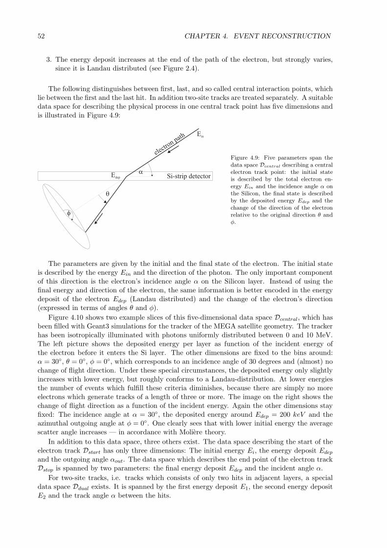
52 CHAPTER 4. EVENT RECONSTRUCTION
3. The energy deposit increases at the end of the path of the electron, but strongly varies,since it is Landau distributed (see Figure 2.4).
The following distinguishes between first, last, and so called central interaction points, whichlie between the first and the last hit. In addition two-site tracks are treated separately. A suitabledata space for describing the physical process in one central track point has five dimensions andis illustrated in Figure 4.9:
Si-strip detector
�
�
Ein
Edep
�
electr
on path
Figure 4.9: Five parameters span thedata space Dcentral describing a centralelectron track point: the initial stateis described by the total electron en-ergy Ein and the incidence angle α onthe Silicon, the final state is describedby the deposited energy Edep and thechange of the direction of the electronrelative to the original direction θ andφ.
The parameters are given by the initial and the final state of the electron. The initial stateis described by the energy Ein and the direction of the photon. The only important componentof this direction is the electron’s incidence angle α on the Silicon layer. Instead of using thefinal energy and direction of the electron, the same information is better encoded in the energydeposit of the electron Edep (Landau distributed) and the change of the electron’s direction(expressed in terms of angles θ and φ).
Figure 4.10 shows two example slices of this five-dimensional data space Dcentral, which hasbeen filled with Geant3 simulations for the tracker of the MEGA satellite geometry. The trackerhas been isotropically illuminated with photons uniformly distributed between 0 and 10 MeV.The left picture shows the deposited energy per layer as function of the incident energy ofthe electron before it enters the Si layer. The other dimensions are fixed to the bins around:α = 30◦, θ = 0◦, φ = 0◦, which corresponds to an incidence angle of 30 degrees and (almost) nochange of flight direction. Under these special circumstances, the deposited energy only slightlyincreases with lower energy, but roughly conforms to a Landau-distribution. At lower energiesthe number of events which fulfill these criteria diminishes, because there are simply no moreelectrons which generate tracks of a length of three or more. The image on the right shows thechange of flight direction as a function of the incident energy. Again the other dimensions stayfixed: The incidence angle at α = 30◦, the deposited energy around Edep = 200 keV and theazimuthal outgoing angle at φ = 0◦. One clearly sees that with lower initial energy the averagescatter angle increases — in accordance with Moliere theory.
In addition to this data space, three others exist. The data space describing the start of theelectron track Dstart has only three dimensions: The initial energy Ei, the energy deposit Edep
and the outgoing angle αout. The data space which describes the end point of the electron trackDstop is spanned by two parameters: the final energy deposit Edep and the incident angle α.
For two-site tracks, i.e. tracks which consists of only two hits in adjacent layers, a specialdata space Ddual exists. It is spanned by the first energy deposit E1, the second energy depositE2 and the track angle α between the hits.

4.4. COMPTON ELECTRON TRACKING 53
[keV]inE2000 4000 6000 8000 10000
[ke
V]
dep
E
50
100
150
200
250
300
350
400
450
500
0
1
2
3
4
5
6
7
8
[keV]inE2000 4000 6000 8000 10000
]° [θ
0
20
40
60
80
100
120
140
160
180
0
0.2
0.4
0.6
0.8
1
1.2
1.4
Figure 4.10: The above pictures show two-dimensional slices of the five-dimensional Dcentral data space of electrontracking. The left picture shows the deposited energy per layer as function of the incident energy of the electronbefore it enters the Si layer; the shape follows a Landau distribution. The right image shows the change of flightdirection as a function of the incident energy. As expected, at high energies Moliere scattering is significantly lesspronounced than at lower energies. The data space has been generated by Geant3 simulations with the MEGAsatellite tracker.
In section 4.4.2.3 an instrument response formulated in terms of those data spaces is used todetermine the direction of motion of tracks via Bayesian electron tracking.
4.4.2 Identification of Compton electron tracks
The greatest challenge for electron tracking is the tracking of Compton electrons at low energies.In this regime, all tracks are short and are heavily influenced by Moliere scattering. As aconsequence, a lot of U-turns can be observed, and only a few tracks appear straight. Thisproblematic domain ranges up to electron energies of 1–2 MeV. At higher electron energies, thetracks get longer and at least the start of the tracks is fairly straight. Thus, the direction canbe found much more easily.
Compton electron tracking is a two-step process: The first step is to figure out all possiblepaths the electron might have taken (see 4.4.2.1), and in a second step the most probablecombination and its direction have to be found (see 4.4.2.2 and 4.4.2.3).
4.4.2.1 Finding all possible track combinations
In order to develop an algorithm that is able to successfully operate on data from a complex real-life detector system, one must always keep in mind how various malfunctions and imperfectionsin the tracker influence the reconstruction. The MEGA prototype in particular has a significantamount of non-working strips, thus the track might have missing hits. A second problem arehigh thresholds leading to missing energy deposits. This is frequently the case at the start ofthe track, when the electron has passed only a small fraction of the layer. High thresholds arealso problematic in the case of hits in one layer whose energy deposit is distributed over severalstrips, with resulting low deposits in individual strips. Finally, additional hits are another sourceof problems. They might originate from noisy channels, from bremsstrahlung emitted by theelectron, or correspond to nearby Compton interactions without causal connection to the trackunder investigation. Figure 4.11 illustrates these issues.
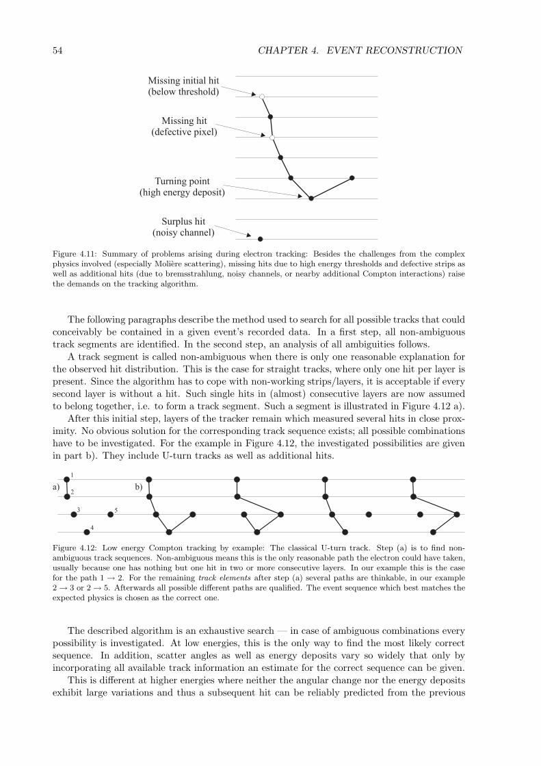
54 CHAPTER 4. EVENT RECONSTRUCTION
Missing initial hit(below threshold)
Missing hit(defective pixel)
Surplus hit(noisy channel)
Turning point(high energy deposit)
Figure 4.11: Summary of problems arising during electron tracking: Besides the challenges from the complexphysics involved (especially Moliere scattering), missing hits due to high energy thresholds and defective strips aswell as additional hits (due to bremsstrahlung, noisy channels, or nearby additional Compton interactions) raisethe demands on the tracking algorithm.
The following paragraphs describe the method used to search for all possible tracks that couldconceivably be contained in a given event’s recorded data. In a first step, all non-ambiguoustrack segments are identified. In the second step, an analysis of all ambiguities follows.
A track segment is called non-ambiguous when there is only one reasonable explanation forthe observed hit distribution. This is the case for straight tracks, where only one hit per layer ispresent. Since the algorithm has to cope with non-working strips/layers, it is acceptable if everysecond layer is without a hit. Such single hits in (almost) consecutive layers are now assumedto belong together, i.e. to form a track segment. Such a segment is illustrated in Figure 4.12 a).
After this initial step, layers of the tracker remain which measured several hits in close prox-imity. No obvious solution for the corresponding track sequence exists; all possible combinationshave to be investigated. For the example in Figure 4.12, the investigated possibilities are givenin part b). They include U-turn tracks as well as additional hits.
a) b)
5
4
3
2
1
Figure 4.12: Low energy Compton tracking by example: The classical U-turn track. Step (a) is to find non-ambiguous track sequences. Non-ambiguous means this is the only reasonable path the electron could have taken,usually because one has nothing but one hit in two or more consecutive layers. In our example this is the casefor the path 1 → 2. For the remaining track elements after step (a) several paths are thinkable, in our example2 → 3 or 2 → 5. Afterwards all possible different paths are qualified. The event sequence which best matches theexpected physics is chosen as the correct one.
The described algorithm is an exhaustive search — in case of ambiguous combinations everypossibility is investigated. At low energies, this is the only way to find the most likely correctsequence. In addition, scatter angles as well as energy deposits vary so widely that only byincorporating all available track information an estimate for the correct sequence can be given.
This is different at higher energies where neither the angular change nor the energy depositsexhibit large variations and thus a subsequent hit can be reliably predicted from the previous

4.4. COMPTON ELECTRON TRACKING 55
ones. The algorithm used in this case is basically the same as that for pair tracking. If the trackis ambiguous, i.e. contains more than one hit per layer, the hit which has the smallest angulardeviation from the direction of the unambiguous track segment is chosen. (In the exampleillustrated in Figure 4.12 a), this algorithm immediately prefers 2 → 3 to 2 → 5.)
For low-energy tracks now a host of possible sequences with two possible directions each (upor down) must be evaluated; in the case of high-energy tracks mostly one sequence with its twopossible directions must be analyzed. In both cases all allowed sequence-direction combinationsfor a given event are now evaluated to find the correct sequence and its direction of motion. Twoapproaches are implemented: a fast, detector-independent figure-of-merits approach and a moresophisticated method based on Bayesian statistics called Bayesian Electron Tracking (BET).
4.4.2.2 Figures-of-merit tracking
Figures-of-merit tracking is a fast and simple approach to find the correct track sequence (in-cluding direction of motion) by calculating a set of quality factors for the track. Those qualityfactors are defined such that the smaller their value, the better the track complies with thephysics of a correct track.
The most relevant indicators are the increase of the deposited energy Edep at the end ofthe track and the increase of the change of the electron direction Δα along the track. Oneapproach, which has been optimized for thinner layers, was introduced by O’Neill (1996). It isbased on comparing measurements with their theoretically expected values. However, initial testhave shown that this method cannot cope with U-turns very well and is thus not followed here.Another approach has been proposed by Nefzger (2000) and Schopper (2001), which suggeststo use the covariances for Edep and Δα to determine the direction of motion. In general, a non-zero covariance shows a relationship between two variables. In our case these pairs of relatedvariables are (1) the deposited energy and the hit ID along the track and (2) the change in thescatter angle along the track and, again, the hit ID along the track.
For the energy increase the covariance is given by:
cov (Edep, i) = Edep · i − Edep · i (4.4)
and for the angle by:cov (Δα, i) = Δα · i − Δα · i (4.5)
The bars indicate averages and the i is the hit number along the track.A positive covariance means that an increase in the hit number is associated with an in-
crease of the scatter angle or energy. For the correct sequence, we expect both cov (Edep, i) andcov (Δα, i) to be positive.
The covariance itself has a physical dimension which arises from the product of their variables,in our case keV or rad. To be able to later combine the two covariances into one figure of merit,the Pearson correlation (e.g. Press, 1992) is used instead of the covariance itself in this work.The Pearson correlation is defined as the covariance divided by the variances of the involvedvariables and can by definition only take values between −1 and +1.
cPearson (Edep, i) =Edep · i − Edep · i√
E2dep − Edep
2√
i2 − i2
(4.6)
cPearson (Δα, i) =Δα · i − Δα · i√
Δα2 − Δα2√
i2 − i2
(4.7)
Obviously cPearson (Δα, i) can only be calculated if the track consists of at least three hits. Thesingle quality factor finally used to pick the most likely electron path is given by:

56 CHAPTER 4. EVENT RECONSTRUCTION
QE,Pearson = 1 − 2 + cPearson (Edep, i) + cPearson (Δα, i)4
(4.8)
The quality factor is normalized such that good tracks have a QE,Pearson close to zero, badtracks values close to one.
The Pearson correlation has one disadvantage: it assumes linear correlations between thetwo variables under consideration. This assumption of course does not hold for Compton elec-tron tracks for either Edep and i or Δα and i. The more general Spearman Rank correlation(e.g. Press, 1992) only assumes a monotone association between the variables and thus is moreappropriate for the problem at hand. The Spearman Rank correlation coefficient is defined as:
cRank = 1 − 6DN3 − N
(4.9)
Here N is the number of elements for which the difference can be calculated, i.e. for the correla-tion coefficient by energy deposit N is one smaller than the total number of track interactions,and for the angular change it is two smaller. D is the sum of the squared difference of the rankseither of Edep and i or of Δα and i:
D (Edep, i) =N∑
n=1
(Rank (Edep,n) − Rank (in))2 (4.10)
Again the correlation coefficient cRank is close to one when the assumption of monotone associ-ation is true. Similar to the Pearson case, the sequence quality factor can be defined as:
QE,Rank = 1 − 2 + cRank (Edep, i) + cRank (Δα, i)4
(4.11)
A discussion of the performance of both approaches can be found in section 4.4.2.4.
4.4.2.3 Bayesian electron tracking
The previous approach has been optimized to be fast and simple. As a consequence, it completelyignores the complex, non-linear response of the detector and it does not use its full dimensionality.In addition, it does not result in a real probability, only in a figure-of-merit.
To assign each track a quality factor that directly reflects its probability of being correctlyreconstructed, the probability p (C| m) needs to be determined. This is the probability thatthe given sequence is correct C given the ordered measurements m. Unfortunately, this valueis not accessible via standard statistical methods — only p ( m|C), the probability to get themeasurement m given that the sequence is correct, is accessible: This probability can easily bedetermined by simulation — or, given enough statistics, from instrument calibration measure-ments.
Bayes’ theorem (Press, 1992) shows a way out of this dilemma: it allows to determine theneeded p (C| m) from p ( m|C) and additional prior information such as p (C), the probability toget a correct sequence, and p ( m), the probability to measure m. This information can also beobtained from calibration or simulation. This approach overcomes both fundamental problemsof the correlation-based methods discussed in the last chapter: the actual probability of correctreconstruction is known, and it is possible to incorporate the full non-linear response of electrontracking through the probability p ( m|C).
For the probability p (C| m) Bayes’ theorem gives:
p (C| m) =p (C) p ( m|C)
p ( m)(4.12)
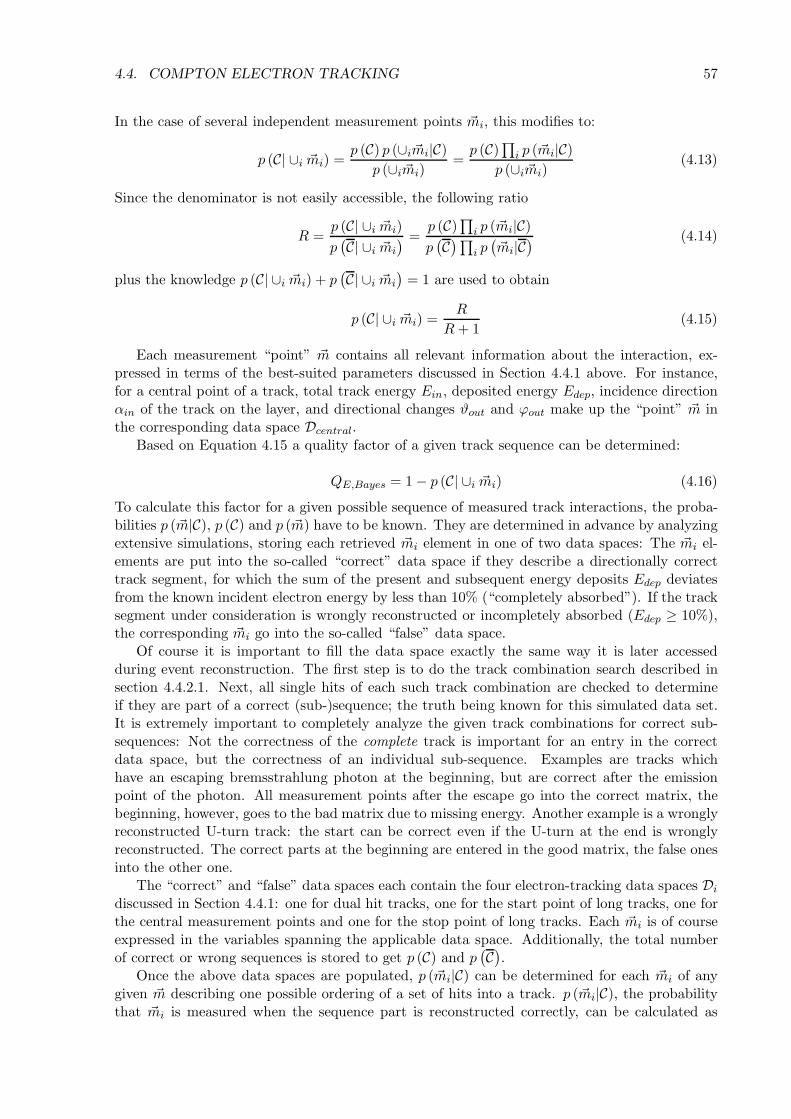
4.4. COMPTON ELECTRON TRACKING 57
In the case of several independent measurement points mi, this modifies to:
p (C| ∪i mi) =p (C) p (∪i mi|C)
p (∪i mi)=
p (C)∏
i p ( mi|C)p (∪i mi)
(4.13)
Since the denominator is not easily accessible, the following ratio
R =p (C| ∪i mi)p(C| ∪i mi
) =p (C)
∏i p ( mi|C)
p(C)∏i p
( mi|C
) (4.14)
plus the knowledge p (C| ∪i mi) + p(C| ∪i mi
)= 1 are used to obtain
p (C| ∪i mi) =R
R + 1(4.15)
Each measurement “point” m contains all relevant information about the interaction, ex-pressed in terms of the best-suited parameters discussed in Section 4.4.1 above. For instance,for a central point of a track, total track energy Ein, deposited energy Edep, incidence directionαin of the track on the layer, and directional changes ϑout and ϕout make up the “point” m inthe corresponding data space Dcentral.
Based on Equation 4.15 a quality factor of a given track sequence can be determined:
QE,Bayes = 1 − p (C| ∪i mi) (4.16)
To calculate this factor for a given possible sequence of measured track interactions, the proba-bilities p ( m|C), p (C) and p ( m) have to be known. They are determined in advance by analyzingextensive simulations, storing each retrieved mi element in one of two data spaces: The mi el-ements are put into the so-called “correct” data space if they describe a directionally correcttrack segment, for which the sum of the present and subsequent energy deposits Edep deviatesfrom the known incident electron energy by less than 10% (“completely absorbed”). If the tracksegment under consideration is wrongly reconstructed or incompletely absorbed (Edep ≥ 10%),the corresponding mi go into the so-called “false” data space.
Of course it is important to fill the data space exactly the same way it is later accessedduring event reconstruction. The first step is to do the track combination search described insection 4.4.2.1. Next, all single hits of each such track combination are checked to determineif they are part of a correct (sub-)sequence; the truth being known for this simulated data set.It is extremely important to completely analyze the given track combinations for correct sub-sequences: Not the correctness of the complete track is important for an entry in the correctdata space, but the correctness of an individual sub-sequence. Examples are tracks whichhave an escaping bremsstrahlung photon at the beginning, but are correct after the emissionpoint of the photon. All measurement points after the escape go into the correct matrix, thebeginning, however, goes to the bad matrix due to missing energy. Another example is a wronglyreconstructed U-turn track: the start can be correct even if the U-turn at the end is wronglyreconstructed. The correct parts at the beginning are entered in the good matrix, the false onesinto the other one.
The “correct” and “false” data spaces each contain the four electron-tracking data spaces Di
discussed in Section 4.4.1: one for dual hit tracks, one for the start point of long tracks, one forthe central measurement points and one for the stop point of long tracks. Each mi is of courseexpressed in the variables spanning the applicable data space. Additionally, the total numberof correct or wrong sequences is stored to get p (C) and p
(C).Once the above data spaces are populated, p ( mi|C) can be determined for each mi of any
given m describing one possible ordering of a set of hits into a track. p ( mi|C), the probabilitythat mi is measured when the sequence part is reconstructed correctly, can be calculated as
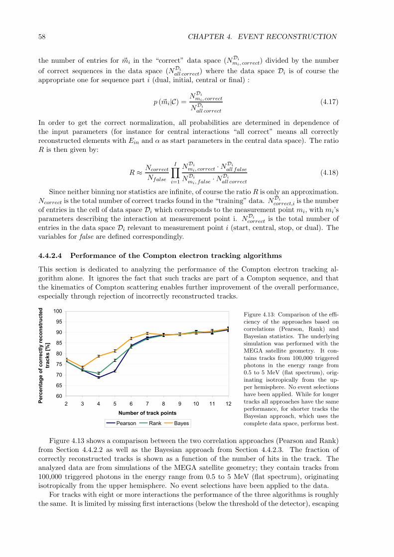
58 CHAPTER 4. EVENT RECONSTRUCTION
the number of entries for mi in the “correct” data space (NDimi, correct) divided by the number
of correct sequences in the data space (NDiall correct) where the data space Di is of course the
appropriate one for sequence part i (dual, initial, central or final) :
p ( mi|C) =NDi
mi, correct
NDiall correct
(4.17)
In order to get the correct normalization, all probabilities are determined in dependence ofthe input parameters (for instance for central interactions “all correct” means all correctlyreconstructed elements with Ein and α as start parameters in the central data space). The ratioR is then given by:
R ≈ Ncorrect
Nfalse
I∏i=1
NDimi, correct · NDi
all false
NDimi, false · NDi
all correct
(4.18)
Since neither binning nor statistics are infinite, of course the ratio R is only an approximation.Ncorrect is the total number of correct tracks found in the “training” data. NDi
correct,i is the numberof entries in the cell of data space Di which corresponds to the measurement point mi, with mi’sparameters describing the interaction at measurement point i. NDi
correct is the total number ofentries in the data space Di relevant to measurement point i (start, central, stop, or dual). Thevariables for false are defined correspondingly.
4.4.2.4 Performance of the Compton electron tracking algorithms
This section is dedicated to analyzing the performance of the Compton electron tracking al-gorithm alone. It ignores the fact that such tracks are part of a Compton sequence, and thatthe kinematics of Compton scattering enables further improvement of the overall performance,especially through rejection of incorrectly reconstructed tracks.
65
69
:5
:9
75
79
;5
;9
855
- # $ 9 6 : 7 ; 85 88 8-
;& ���������������#��
*��#��������������!����#���&��$�
�������7:8
.����� <�, ���
Figure 4.13: Comparison of the effi-ciency of the approaches based oncorrelations (Pearson, Rank) andBayesian statistics. The underlyingsimulation was performed with theMEGA satellite geometry. It con-tains tracks from 100,000 triggeredphotons in the energy range from0.5 to 5 MeV (flat spectrum), orig-inating isotropically from the up-per hemisphere. No event selectionshave been applied. While for longertracks all approaches have the sameperformance, for shorter tracks theBayesian approach, which uses thecomplete data space, performs best.
Figure 4.13 shows a comparison between the two correlation approaches (Pearson and Rank)from Section 4.4.2.2 as well as the Bayesian approach from Section 4.4.2.3. The fraction ofcorrectly reconstructed tracks is shown as a function of the number of hits in the track. Theanalyzed data are from simulations of the MEGA satellite geometry; they contain tracks from100,000 triggered photons in the energy range from 0.5 to 5 MeV (flat spectrum), originatingisotropically from the upper hemisphere. No event selections have been applied to the data.
For tracks with eight or more interactions the performance of the three algorithms is roughlythe same. It is limited by missing first interactions (below the threshold of the detector), escaping
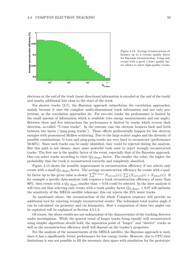
4.4. COMPTON ELECTRON TRACKING 59
E, BayesQ
-310 -210 -110 1
Ave
rag
e re
con
stru
ctio
n e
ffic
ien
cy [
%]
0.8
0.85
0.9
0.95
1
Figure 4.14: Average reconstruction ef-ficiency up to a certain quality factorfor Bayesian reconstruction: Using onlyevents with a good (=low) quality fac-tor allows to select high-quality events.
electrons at the end of the track (most directional information is encoded at the end of the track)and nearby additional hits close to the start of the track.
For shorter tracks (2-7), the Bayesian approach outperforms the correlation approaches,mainly because it uses the complete multi-dimensional track information and not only pro-jections, as the correlation approaches do. For two-site tracks the performance is limited bythe small amount of information which is available (two energy measurements and one angle).Between three and five interactions the performance is limited by tracks which reverse theirdirection, so-called “U-turn tracks”. In the extreme case the electron bounces back and forthbetween two layers (“ping-pong tracks”). Those effects preferentially happen for low electronenergies with pronounced Moliere scattering. Due to the large scatter angles and the diversity ofpossible combinations, U-turn and ping-pong tracks are very hard to reconstruct (performance50-60%). Since such tracks can be easily identified, they could be rejected during the analysis.But this path is not chosen, since more powerful tools exist to reject wrongly reconstructedtracks. The first one is the quality factor of the event, especially that of the Bayesian approach.One can select tracks according to their QE,Bayes factor. The smaller the value, the higher theprobability that the track is reconstructed correctly and completely absorbed.
Figure 4.14 shows the possible improvement in reconstruction efficiency if one selects onlyevents with a small QE,Bayes factor. The average reconstruction efficiency for events with a qual-ity factor up to the given value is shown:
∑QE,Bayes
0 Ncorrect(x)/∑x
0 (Ncorrect(x) + Nfalse(x)). Iffor example a specific data-analysis task requires a track reconstruction efficiency of more than90%, then events with a QE,Bayes smaller than ∼ 0.04 could be selected. In the later analysis itwill turn out that selecting only events with a track quality factor QE,Bayes < 0.07 will optimizethe sensitivity of the MEGA satellite telescope; this cut rejects the 25% worst tracks.
As mentioned above, the reconstruction of the whole Compton sequence will provide anadditional tool for rejecting wrongly reconstructed events: The redundant total scatter angle ϑcan be calculated via geometry and via kinematics. How a comparison of these two angles canbe exploited will be explained in Section 4.5.1.2.
Of course, the above results are not independent of the characteristics of the tracking detectorunder investigation. While the general trend of longer tracks being equally well reconstructedusing simpler algorithms should hold, the separation point of “longer” and “shorter” tracks aswell as the reconstruction efficiency itself will depend on the tracker’s properties.
For the analysis of the measurements of the MEGA satellite, the Bayesian approach is used,since it has a significantly better performance for low energy tracks. However, due to CPU-timelimitations it was not possible to fill the necessary data space with simulation for the prototype.

60 CHAPTER 4. EVENT RECONSTRUCTION
4.4.2.5 Can electron tracking be improved further?
Especially the Bayes algorithm has already reached a high level of performance. Increasingthe reconstruction efficiency by another few percent would certainly require exponentially morework than has been invested up to this point. Most failures are due to extreme measurementsor unfortunate geometries (e.g. large electron incidence angles, tracks with U-turns, high energydeposits corresponding to the tails of the Landau distribution, etc.) and detector imperfections(escaping electrons, passive material, non-zero thresholds, etc.).
The most problematic category of events for the current algorithm are small U-turn tracks,i.e. tracks with have large initial incidence angles and move sideways through their “birth-layer”and return to their original layer. A possibility to improve their handling would be to give themtheir own data space in the Bayesian approach. Currently the central data space of Bayesianelectron tracking is mainly filled with long straight tracks, where U-turns are unusual and thushave a lower probability. For four-hit tracks one could think of three data spaces: one wherefour layers are hit (straight tracks), a second where three layers are hit (circular tracks) anda third where two layers have been hit (ping-pong tracks). The same can be done for curlingthree-hit tracks. Due to the tremendous overhead and the large simulation runs required to getenough statistics, this remains a task for a future satellite mission.
In terms of detector design, thinner layers would be advantageous to address the problemof U-turn tracks. Less Moliere scattering makes the tracks straighter. However, the problemis not eliminated, it is only shifted down to lower energies. In addition, one would need morelayers to achieve the same scatter probability and consequently the energy measurement errorwould increase since the track of an electron with given energy would be recorded in to moremeasurement points.
The most relevant information for finding the direction of the track is encoded in the startpoint of the track. As already mentioned, the Compton interaction takes place somewhere insidethe first layer and thus the electron deposits less energy than it would if it passed through thecomplete layer. As a consequence, it is extremely important to have low enough thresholds tomeasure the start point of the track — its low energy deposit distinguishes the start from theend of the track. In addition, if one does not measure the start of the track and thus not knowthe real location of the Compton interaction, the imaging of the whole Compton event is alsodeteriorated, because the direction of the scattered gamma-ray has a non-neglectable error.
Another important point is to build the tracker large enough that most electrons are con-tained in it. An ideal satellite tracker would contain thicker Silicon layers, or even Germaniumor CZT layers, at the bottom to stop the electrons. This would also be relevant for the sides ofthe tracker.
For the energy measurement it is also necessary to have as little passive material and as fewdefective strips/pixels in the detector as possible. Both facts cause missing hits, thus leaks ofenergy and holes in the tracks.
4.5 Compton sequence reconstruction
In the preceding steps all easily identifiable structures in the tracker have been found: If pairsor high-energy charged particles were found then the event reconstruction never reached thisstep. In addition, all Compton recoil electron tracks have already been located and sequencedin the previous step. Tracks are now considered as one interaction whose position is the startpoint of the track. In order to successfully perform the next step, i.e. to identify and sequenceCompton interactions, the reconstruction’s focus must now broaden to also include all isolatedhits recorded as part of an event. For MEGA, events are defined by trigger criteria to consistof at least one interaction in the tracker and at least one interaction in the calorimeter.

4.5. COMPTON SEQUENCE RECONSTRUCTION 61
Compton sequence reconstruction searches for the true path of the initial gamma ray byanalyzing all possible permutations of the recorded interactions and assigning a Compton qualityfactor to each permutation, which is based on the probability that an event actually occurredin this way. The permutation with the best quality factor is chosen as the correct sequence ofinteractions. If the best quality factor is not better than a certain value, the event can of coursebe rejected. This last decision, however, is not made during event reconstruction, but — as acut on the Compton quality factor — in the later high-level data analysis.
The only outright event rejection happening in the present step concerns events for whichthe Compton kinematics are not correct for any one of the possible permutations or for whichthere are too many interactions to analyze: normally events with eight interactions or more areno longer analyzed, because it would require analyzing 8! = 40320 possible permutations andthus far too much CPU time. The fraction of completely absorbed Compton events with morethan seven interactions is negligible for MEGA.
In the following, first the basic principles for sequencing Compton interactions are presented.Afterwards, two different implementations of these principles are discussed: the Classic Comp-ton Sequence Reconstruction (C-CSR) and the Bayesian Compton Sequence Reconstruction (B-CSR). The goal is again to have one fast approach, which can be applied to all geometries withoutpreparations (C-CSR), and one optimized method, which considers the (almost) complete dataspace of the telescope but requires extensive simulations (B-CSR).
4.5.1 Characteristics of the data space
Compton scattering is described by the Klein-Nishina equation. A wide range of different energytransfers to the Compton electron is possible, and consequently the electron might or might notgenerate a track. The scattered gamma ray might undergo another Compton interaction, itmight be stopped by photo absorption, if its energy is above 1.022 MeV it could undergo a paircreation, or it might even Rayleigh scatter. Since in the last process no energy is deposited,this is of course not detectable as interaction. Even leaving out the highly unlikely combinationof a Compton scatter followed by a pair-creation event and ignoring Rayleigh scattering asboth not significant and not detectable, a MEGA-style tracking Compton telescope measures awide variety of different Compton event types which all require slightly different reconstructionapproaches:
1. Simple COMPTEL-type events have one hit without a track in the first detector andanother hit in the second detector. For most of these events it is impossible to determinethe direction of motion of the photon since for MEGA the time of flight between theinteractions cannot be measured.
2. If the event consists of one track and one hit in the calorimeter, then the redundantinformation provided by the track allows to determine the direction of motion of thephoton.
3. The third type is characterized by multiple (3+) Compton interactions. Having severalCompton interactions results in redundant information about the kinematics, which caneither be used for determining the sequence of the interactions or — if the sequence isknown or at least four interactions exist — of the total energy. This type can also havetracks, which further helps to find the correct sequence.
In general, the more information is available about the event, the higher the probability thatthe event can be reconstructed correctly.

62 CHAPTER 4. EVENT RECONSTRUCTION
4.5.1.1 Two interactions without track
When no additional information is available, the direction of motion of completely absorbed two-site events can only be retrieved unambiguously in rare cases. Those occur when the conditionsof Equations 2.7 are met for one direction (top-bottom), but not for the other direction (bottom-top), i.e. when the energy transfer to the electron is smaller than the minimum allowed gamma-ray energy in case of backscattering. The small areas in the data space in which this holds areillustrated in Figure 4.15. The black area represents events going top to bottom and the darkgray line those going bottom to top. In all the unambiguous cases, there is only a very smallenergy transfer to the recoil electron. Thus this data space is partly complementary to the dataspace of tracked events.
Energy incoming gamma-ray [keV]0 1000 2000 3000 4000 5000
Bot
tom
ene
rgy
depo
sit [
keV
]
0
1000
2000
3000
4000
5000
Both sequences are invalid
Both sequences are valid:Large ambiguous area
Only top-botto
m is valid
Only bottom-top is valid
Figure 4.15: The black area is occupiedby Compton interactions for which thedirection of motion of the photon canbe determined merely from the energydeposits as “top to bottom” and thedark gray area indicates photons mov-ing unambiguously “bottom to top” –of course under the assumption of com-plete absorption. In the (light grey)space between those areas, both direc-tions of motion are allowed. The areaabove the black line as well as a smallarea below 0.5E0 do not contain validevents. In the former case, a single en-ergy deposit would already be largerthan the energy of the incoming pho-ton; the latter area is forbidden be-cause of the constraints on allowableelectron and photon energies resultingfrom Equations 2.7: For instance, foran incoming 100 keV photon, only 0–30 keV can be transferred to the elec-tron.
The absolute positions of the interactions — as opposed to the angles between them —are another piece of information. These allow to determine the interaction probabilities ofthe photon on its path to the measured interaction locations. Due to the complexity of thegeometry and the ambiguity in incident photon direction arising from the Compton cone, theabsorption probability towards the initial interaction location is difficult and thus CPU-intensiveto determine. Therefore it is not used in the current analysis. The absorption probabilitybetween the first and the second interaction is easily accessible. Successfully applying it to theevent reconstruction, however, requires an excellent position resolution in both detectors in orderto know the intervening material in the complex geometry of a real detector. Unfortunately,MEGA’s calorimeters do not provide sufficiently fine position resolution. Thus, this informationis only of limited use for MEGA and only included in the more complex Bayesian approach (seeSection 4.5.3). In that section, it will also be shown that absorption probabilities are bettersuited to rejecting (strange) sequences (with e.g. random hits with low energy deposits) thanto distinguishing between two equally valid sequences with roughly equal energy deposits in thetwo interactions points. Also the distribution of the Compton scatter angles according to theKlein-Nishina cross section encodes information about the direction of motion, even though thisis also a weak criterion.
Finally, the available information about two-site events without track does not really allowto verify the quality of those events. In particular, it is not possible to determine if they are

4.5. COMPTON SEQUENCE RECONSTRUCTION 63
completely absorbed or not. Only an approach which uses the complete information about thedetection process in the instrument can make use of those events.
4.5.1.2 Two interactions with track
For two-site events with track MEGA can rely on the electron track to find the direction ofmotion of the gamma ray. The most frequent class of background events which have to berejected in a satellite in low-earth orbit are gamma rays originating from the earth’s atmosphere,so-called albedo photons. For a discussion of satellite background components and their origins,see Section 10.2.1. In the case of tracked two-site albedo-photon events, photons interact oncein the calorimeter, then produce a track in the Silicon. Most likely, they then escape from thedetector — if they are stopped in the tracker, they are unlikely to produce a track, because thenecessary photo absorption happens only at very low photon energies. Figure 4.16 illustratessuch an event.
�r
k
�m
k
gk
ek
Ek
El
real
real
Figure 4.16: A typical upward-moving gamma rayin the MEGA detector: The first interaction (in-dex l) happens in the calorimeter, a second one(index k) in the tracker, and the scattered gamma-ray escapes. Here ek is the (correct) direction ofthe recoil electron, gk is the (wrong) direction ofthe scattered gamma-ray, ϑm
k is the wrong and ϑrk
is the correct total scatter angle. El and Ek arethe two measured energy deposits. It is assumedthat the electron-tracking algorithm has identifiedthe direction of motion of the electron correctly.
In the low-earth orbit forseen for a MEGA satellite, the albedo photons originate mainly fromaround 120 degree zenith distance, since they are generated in the earth’s upper hemisphere.Thus, the originally envisioned approach of simply rejecting all events with upward-movingelectron tracks — feasible for photons truly coming from the back of the instrument — will notreject albedo photons well; a more sophisticated approach is necessary.
The key to this is the total scatter angle ϑ, which is the angle between the direction ofthe scattered gamma-ray gk and the direction of the recoil electron ek (see Figure 4.16). Thisinformation is redundant — ϑ can be determined via kinematics (identical with Equation 2.8)
cos ϑkink =
Ek(El + E0)
El
√E2
k + 2EkE0
(4.19)
and, using the information the electron track provides, also via geometry
cos ϑgeok =
gk · ek
| gk| | ek| (4.20)
If there is a large discrepancy dϑ = ϑkink − ϑgeo
k between the two angles, then the assumedordering is likely to be wrong, or the event is incompletely absorbed. This is called the dϑ-criterion. Unfortunately, for the thick tracker layers of MEGA and for low electron energies itis also likely that the electron has simply undergone strong Moliere scattering, which results inlarge dϑ values as well, or that the electron track orientation has been determined incorrectly.Such events, however, will not appear in the center of the point spread function of a source andthey should receive a bad quality factor for later rejection.

64 CHAPTER 4. EVENT RECONSTRUCTION
Similar values of ϑkin and ϑgeo, however, do not automatically mean that the ordering iscorrect! Figure 4.17 shows values of dϑ (z-axis, color) for upward moving gamma-rays at 2 MeVand at 10 MeV, based on the wrong assumption of a downward moving photon: the energyin the track is assumed as the initial deposit (“wrong electron energy”) and the deposit inthe calorimeter as the second deposit (“wrong gamma energy”). The main cause for dϑ �= 0 incorrectly reconstructed events is Moliere scattering. In order not to reject too many valid events,only dϑ values larger than ∼35◦ (for 2 MeV photos, depending of course on the electron energy,with smaller values for higher energies) can be considered a reliable indication that somethingis wrong with the event.
Note that there exists a large region with very small variations in dϑ (at small Eg and/orEe). In this region, both directions are valid within the limits of Moliere scattering and thus onecannot distinguish between an incompletely absorbed upward-moving photon and a completelyabsorbed downward-moving photon. The ambiguity for low electron energies (small “wrongrecoil electron energy”) in the data space of two-site events with tracks is not relevant forMEGA — at those energies no tracks are generated. Ambiguities also exist for low depositsin the calorimeter (small “wrong scattered gamma-ray energy”); these can be eliminated byappropriate event selections.
Since the direction of motion cannot be determined uniquely everywhere in the data space,electron tracking — without additional information — is not as powerful a direction-of-motiontool as measuring the time-of-flight would be. However, electron tracking has of course an-other great advantage: it significantly reduces the size of the point-spread function, markedlyimproving a satellite instrument’s sensitivity.
Wrong recoil electron energy [keV]0 500 1000 1500 2000
Wro
ng s
catte
red
gam
ma
ener
gy [k
eV]
0
500
1000
1500
2000
0
20
40
60
80
100
Not filled due to original Compton processes
Rejected by Compton kinematics
Good rejection capability
Bad rejection capability
[deg]ϑd
Wrong recoil electron energy [keV]0 2000 4000 6000 8000 10000
Wro
ng s
catte
red
gam
ma
ener
gy [k
eV]
0
2000
4000
6000
8000
10000
0
20
40
60
80
100
120
140
Good rejection capability
Bad rejection capability
[deg]ϑd
Figure 4.17: This figure shows the difference between the total scatter angle ϑ measured via geometry and viakinematics for an upward moving and escaping gamma ray which has its first interaction in the calorimeter for2 MeV photons (left) and for 10 MeV photons (right). dϑ is calculated (wrongly) assuming the first interactionhappened in the tracker. For a large area in the data space such events can be rejected because they have largedϑ values. However, low electron energies and/or low scattered gamma-ray energies also result in small ϑ values.Such wrongly reconstructed events cannot be distinguished from correct ones via the dϑ-criterion.
The track information cannot only be used to determine the direction of motion of thephoton. Applying a dϑ selection also serves to reject incompletely absorbed events which movefrom tracker to calorimeter, since ϑkin
k is wrong for such events. This is of course again limitedby Moliere scattering, and one therefore has to allow for a sufficiently large tolerance in dϑ.Figure 4.18 shows the theoretical variation in the difference of the two ϑ’s when the scatteredgamma ray is incompletely absorbed (left column) and when the recoil electron is incompletelyabsorbed (right column) for 2 MeV (top row) and 10 MeV (bottom row) incoming gamma rayswhich first interact in the tracker. In this context incomplete absorption means that not allenergy is deposited in active material, i.e. the particle either escapes or deposits its energy inpassive material.

4.5. COMPTON SEQUENCE RECONSTRUCTION 65
Electron energy [keV]0 500 1000 1500 2000In
com
plet
e G
amm
a en
ergy
[keV
]
0
500
1000
1500
2000
0
20
40
60
80
100
Not filled due to Compton kinematics
Good rejection capability
Bad rejection capability
[deg]ϑd
Incomplete Electron energy [keV]0 500 1000 1500 2000
Gam
ma
ener
gy [k
eV]
0
500
1000
1500
2000
0
10
20
30
40
50
60
70
Not filled due to Compton kinematics (back scattering)
Good rejection capability
Bad rejection capabilitykinϑ < dgeoϑd
[deg]ϑd
Wrong recoil electron energy [keV]0 2000 4000 6000 8000 10000
Wro
ng s
catte
red
gam
ma
ener
gy [k
eV]
0
2000
4000
6000
8000
10000
0
20
40
60
80
100
120
140
Good rejection capability
Bad rejection capability
[deg]ϑd
Incomplete Electron energy [keV]0 2000 4000 6000 8000 10000
Gam
ma
ener
gy [k
eV]
0
2000
4000
6000
8000
10000
0
10
20
30
40
50
60
70Good rejection capability
Bad rejection capability
kinϑ < dgeoϑd
[deg]ϑd
Figure 4.18: This figure shows the difference between the total scatter angle ϑ measured via geometry and viakinematics for downward-moving photons. In the left column, the scattered gamma ray is incompletely absorbed,in the right column the recoil electron is incompletely absorbed. Since Moliere scattering induces significant dϑin good events, for MEGA at 2 MeV (top row) rejections are possible for dϑ values above ∼ 35 degrees, and ∼10 degrees at 10 MeV (bottom row). Thus, it is only possible to reliably reject incompletely absorbed events insmall portions of the data space. In the idealized, error and Moliere-scattering free data space illustrated above,ϑ is exactly zero for the completely absorbed events (diagonal line).
Unfortunately, the total scatter angle ϑ changes only very slowly with decreasing energy ofthe scattered photon. This is the case because the calculated scatter angles of electron andphoton move in opposite directions: the Compton scatter angle ϕ gets larger while the electronscatter angle ε gets smaller. As a consequence, the area for which there is a significant difference(relative to the effects of Moliere scattering) between the geometrically determined (the correct)and the energetically determined total scatter angle is small. For the largest part of the dataspace it is impossible to flag incompletely absorbed events. Thus it is crucial to completelyabsorb most of the the incoming gamma rays: the detector must have a large active to passivemass ratio and must be thick enough to stop all photons.
A final remark: In theory it would also be possible to use the redundant track informationto determine the original gamma-ray energy for incompletely absorbed events. However, forMEGA this would result in multiple problems: First, correcting the energy — without know-ing the interaction sequence — would upgrade all upward-moving photons to energy-correcteddownward-moving photons and thus dramatically increase the background. Second, this methodwould only work for the highest-energy photons (beyond 15 MeV) due to the limitation fromMoliere scattering. Finally, at those high energies in almost all cases the recoil electron as well asthe scattered gamma-ray are not completely absorbed, finally rendering a correction impossible.
4.5.1.3 Multiple Compton interactions
The next level of complexity is reached when there are more than two interactions: at least twoCompton interactions and one final complete (photo) absorption. Figure 4.19 illustrates suchan event.
If one ignores tracks, then the complete data space for multiple Compton events consists of N

66 CHAPTER 4. EVENT RECONSTRUCTION
El
Em
Ek
dk
dl
�k
�l
�k
gl
gi
gk
ek
el �l
Figure 4.19: Multiple Compton interactions: In this example a gammaray undergoes three interactions: Compton scattering at positions k and l,as well as a photo absorption at position m. The solid line corresponds tothe path of the gamma ray, the dotted lines are the paths of the electrons.The plotted event contains several independent and redundant pieces ofinformation. First, the second Compton scatter angle ϕl can be calculatedin two ways: via Compton kinematics (Equation 4.21) and via interactiongeometry as angle between gk and gl (Equation 4.22). In addition, twoelectron tracks also provide redundant information: Each of the totalscatter angles ϑk and ϑl can be calculated via Compton kinematics andvia the interaction geometry as angle between the photon direction gk (gl)and the electron direction ek (el). This redundant information allows todetermine the interaction sequence and (sometimes) whether or not thephoton’s energy is completely absorbed.
measurement points (with x, y, z and energy), which would lead to a 4·N -dimensional data spacematrix. The size of such a data space rapidly increases for Compton events consisting of severalinteractions. In addition, the absolute interaction positions x, y, z are not directly linked to theunderlying physics. A well-designed data space thus is spanned by parameters that are directlyconnected to the underlying physics. The data space must be designed to conserve as muchinformation as possible while not exceeding a manageable number of dimensions. Therefore,the parameters spanning the data space should be as independent as possible of one another.Particular care must be taken to conserve all information which is useful to discriminate betweenpossible paths of the photon, and to determine the likelihood of an event being fully absorbed.Separate data spaces for first, central, and last interactions can be designed similar to theapproach taken during electron tracking. In the following, parameters suited to these tasks arediscussed; starting from these eventually a data space for Compton event reconstruction will bebuilt.
As in the case of electron track reconstruction, in the process of reconstructing a Comptonevent one has to investigate all different paths (= sequences) the particle — in this case thephoton — might have taken. In general, there exist N ! possible paths (= permutations). If oneconsiders a triple interaction, 6 permutations have to be investigated to figure out the correctsequence.
For this task the Compton scatter angle ϕl of the central Compton interaction from Figure4.19 has proven most valuable. Just like the total scatter angle (ϑk or ϑl) for electron tracking,this information can be calculated in two ways from the redundant information available: Viakinematics (similar to the classic Compton equation 2.6):
cos ϕkinl = 1 − E0
El++
E0
El+ + El(4.21)
and via geometry, as the angle between the photon direction before and after interaction l:
cos ϕgeol =
gk · gl
| gk| | gl| (4.22)
Here El is the energy deposit at interaction site l, which corresponds to the energy of the recoilelectron of the Compton interaction l, and El+ is the energy of the scattered photon, which isdefined as all energies deposits after interaction l in the sequence: El+ =
∑Nj=l+1 Ej . For the
example in Figure 4.19 this is simply Em.

4.5. COMPTON SEQUENCE RECONSTRUCTION 67
In the case of the correct permutation, cosϕkinl and cos ϕgeo
l should be identical withinmeasurement errors. Compared to electron tracking, where a large dϑ (∼ 35◦ at 2 MeV) hadto be accepted because of the large uncertainty due to Moliere scattering, the tolerated dϕ =ϕkin
l −ϕgeol are much smaller: They correspond to the angular resolution, determined by energy
resolution, position resolution and Doppler broadening. For MEGA, good dϕ values are a fewdegrees if the interactions happen in the tracker, but unfortunately the deviations are muchworse in the calorimeter due to its limited position resolution (in the rare extreme case up to90◦ in the side calorimeter).
The dϕ-criterion — as the dϑ-criterion for electron tracks — cannot completely competewith time-of-flight information concerning the determination of the direction of motion: Thedirection of motion cannot always be determined uniquely from dϕ. The most obvious exampleis the case of three hits with the same energy. For two of the calculated sequences — theoriginal one and its reverse — the dϕ are zero. In this case only additional information such asabsorption probabilities can help to determine the correct sequence.
Figure 4.20 shows dϕ for a 2 MeV photon which undergoes a triple Compton interaction asa function of the first and the third energy deposit. Only one of the five wrong sequences isconsidered, the reverse one. In case of very small second energy deposits as well as in the case ofequal first and third deposits (within measurement errors and Doppler broadening), the reversecannot be distinguished from the correct sequence: In both cases dϕ is close to zero for the trueas well as the reverse order.
While for this figure only two sequences where considered, in reality all N! permutationshave to be investigated. This further increases the risk that one wrong combination by chanceis better than the original one due to the limited energy resolution.
Another illustration of ambiguous data space regions is shown in Figure 4.21. For givenenergy deposits (in the example E1 = 200 keV, E2 = 1200 keV, E3 = 600 keV) the distance ofthe interactions are varied and thus the ϕgeo of a wrong sequence. Moving one position leads toa monotone increase (or decrease) of the ϕgeo value (in the case of a wrong sequence — ϕgeo ofcourse stays constant for the correct sequence). Obviously if during this process ϕgeo gets closeto the value of ϕkin, determining the sequence is ambiguous.
While the dϕ-criterion is the strongest for finding the true sequence of multiple Comptoninteractions, and therefore constitutes an obvious first choice of a parameter used to span theCompton reconstruction data space, it is not the only criterion which can be used — the eventsin ambiguous sections of the data space are not lost!
For MEGA the most obvious and strongest additional information is of course the electrontrack, which allows the application of the ϑ-criterion to 3+ interaction events in the same way asdescribed in the last chapter for two-site interactions with tracks. If no tracks are measured, thenstill the absorption probabilities on the paths between the interactions, the distributionof ϕ according to the Klein-Nishina equation, as well as variations in the occupation of the dataspace induced by a particular instrument’s geometry can be used to differentiate between thecorrect and wrong sequences.
Those features can best be shown in a data space filled by simulations of photons fromall directions incident on a real-instrument geometry, in this case the MEGA satellite. Theillustrations in Figure 4.15 through 4.21 were generated from analytic calculations. The fulldata space underlying the projections shown in the subsequent images is that used for theBayesian event reconstruction discussed later in this Chapter (Section 4.5.3).
Figure 4.22 illustrates the dependence between gamma-ray energy and absorption probabilityen route towards the last interaction point in a Compton sequence. (Similar to the approachtaken for electron tracking, the data spaces used for first and last interaction are somewhat

68 CHAPTER 4. EVENT RECONSTRUCTION
First deposit [keV]0 500 1000 1500 2000
Thi
rd d
epos
it [k
eV]
0
500
1000
1500
2000
1
10
210
[deg]ϕd
Good rejection capability
Bad rejection capability
Distance first to second interaction [cm]0 2 4 6 8 10
Dis
tanc
e se
cond
to th
ird in
tera
ctio
n [c
m]
0
2
4
6
8
10
2
4
6
8
10
12
14
16
18
20
22
[deg]ϕd
Figure 4.20: One of the regions in the triple Comptondata space where calculating the Compton scatter an-gle difference dϕ = |ϕkin − ϕgeo| is not sufficient tounambiguously determine the direction of motion ofthe gamma ray: the approach is in trouble when firstand third deposit have equal energy within measure-ment errors or when the third deposit is very small.To calculate dϕ only one sequence has been consid-ered, the one reverse to the correct one.
Figure 4.21: Another illustration of the limitationsof the triple-Compton method: If one looks at oneenergy signature (in this case E1 = 200 keV, E2 =1200 keV, E3 = 600 keV) and varies the distance be-tween the interactions (which results of course in dif-ferent geometrical scatter angles for the wrong se-quences but does not vary them for the correct se-quence), ambiguous data space regions become evi-dent. The given example is a fairly bad case.
Pa
0 0.2 0.4 0.6 0.8 1
[ke
V]
tot
E
210
310
1
10
210
310
410
510
counts
Pa
0 0.2 0.4 0.6 0.8 1
[ke
V]
tot
E
210
310
1
10
210
310
410
510
counts
Figure 4.22: Remaining photon energy as a function of the absorption probability towards the last interactionpoint. The left image shows this distribution for correct sequences, the right image for all wrong sequences.The data spaces look rather similar, with one exception: the “false” one has some excesses at high energies andlow probabilities as well as at low energies and high probabilities. The underlying simulation was performed forphotons from all directions incident on the MEGA satellite geometry. Since this data space is generated as partof the Bayesian CSR, additional details can be found in Section 4.5.3.
different from that relevant to central interactions.) The left figure shows only the correctsequences, the right figure only the wrong sequences. Ideally, the good sequences would occupycompletely different regions in the data space than the wrong sequences, and thus they could beeasily distinguished. But partially due to the large position measurement errors of the MEGAdetector, the differences are marginal. Clear excesses can only be found at high energies and lowprobabilities, as well as at low energies and high probabilities. In the first case the sequence had

4.5. COMPTON SEQUENCE RECONSTRUCTION 69
[deg]ϕd
-110 1 10 210
[d
eg]
kin
ϕ
0
20
40
60
80
100
120
140
160
180
1
10
210
310
410
counts
[deg]ϕd
-110 1 10 210
[d
eg]
kin
ϕ
0
20
40
60
80
100
120
140
160
180
1
10
210
310
410
counts
Figure 4.23: Compton scatter angle ϕkin as a function of the scatter angle difference dϕ. Again, the image on theleft shows only the correct sequences, the one on the right the all wrong sequences. The correct sequences gatherat low dϕ, but due to ambiguities resulting from the problems of the multiple Compton approach as well as thelimited energy and position resolution of the simulated MEGA satellite, wrong sequences occupy that space aswell. The distribution on the y-axis is determined by the Klein-Nishina distribution of ϕ and the geometry. Theunderlying simulation is a necessary ingredient to the Bayesian reconstruction; details can be found in Section4.5.3.
a too-small interaction distance for a large photon energy, in the latter the sequence had a too-large distance for a small photon energy. Only wrong sequences with those characteristics can berejected by an absorption probability criterion. Using this criterion for stricter event selectionsone would immediately risk to also reject good event sequences, because the correspondingdata-space regions overlap.
The distribution of simulated events as a function of ϕkin and dϕ is shown in Figure 4.23.Again, the left image shows only the correct sequences, while the right image shows all otherpermutations. The first obvious finding is that the good sequences gather at low dϕ and theirdistribution is determined by the angular resolution of the telescope (large scatter angles resultin worse angular resolution). The wrong sequences mainly gather at large dϕ values, but —due to the previously described ambiguities — stretch out to small dϕ. In ϕkin the distributionof good sequences is modulated by the Klein-Nishina distribution of the Compton scatter angleand by the geometrical factors. Due to the large ambiguous regions it is not always possible todetermine the correct sequence, since it is likely that by chance one of the wrong sequences hassimilar geometrical and kinematical Compton scatter angles and thus a small dϕ.
In case of four (or more) interactions, in theory the redundant information could also beused to determine the energy of incompletely absorbed events. For each triplet of interactionsthe incoming energy in the triplet can be calculated independent of subsequent interactions orthe total deposited energy:
Etot,1 = E1 + 0.5E2 + 0.5√
E22 + 4E0E2/(1 − cos(ϕ2)). (4.23)
In case of four interactions, for each possible sequence two triplets exist for which the totalenergy can be calculated. This results again in redundant information: dE = Etot,1 −Etot,2 hasto be ∼0 if the reconstructed sequence and the determined incoming photon energy are correct.
Unfortunately, the ambiguities in determining the total energy of incompletely absorbedevents are large. An excellent position and energy resolution would be required to estimate the
70 CHAPTER 4. EVENT RECONSTRUCTION
total energy correctly. Since these requirements are not fulfilled by the present MEGA detectorsthis avenue is not explored further.
In summary, a good data space to describe Compton interactions should comprise the anglesdϕ and ϕ as well as the photon energy Ei in order to allow use of the dϕ-criterion as wellas the distribution of the Compton scatter angle according to the Klein-Nishina equation. Inaddition, a distance factor d is needed, which describes the geometrical uncertainty influencingϕ. If electron tracks are present, dϑ and ϑ are needed as well. The absorption probability ofthe incident photon on its way to the interaction as a function of the photon energy adds avaluable tool to reject wrong sequences. In addition, of course the detector type (this encodesinformation about energy resolution, position resolution, Doppler broadening, etc.) as well asthe number of interactions in the event must be retained. The exact layout of such a data spaceused for event reconstruction can be found in Section 4.5.3.
4.5.2 Classic Compton sequence reconstruction
The last section explained in detail the signatures of different event types — first for two-siteinteractions without tracks, then for two-site interactions with tracks, and finally for multiple-siteinteractions. This and the following section are now concerned with making use of the knowledgegained in order to reconstruct different types of Compton events as well as to determine thecertainty with which a given event was reconstructed correctly. In this section, a straightforward,analytical approach is used — the “Classic” Compton reconstruction.
The part of the classic approach concerned with non-tracked, multiple-Compton events hasalready been described in the literature by different authors for different applications, for e.g.nuclear spectroscopy (van der Marel and Cederwall , 1999; Schmid et al., 1999) as well as gamma-ray astronomy (Oberlack et al., 2000b; Boggs et al., 2000a). In this work it has been extendedto electron tracking.
Two-site events without track Without the information of time-of-flight and under high-background conditions, determining the order of two-site events is a non-trivial task. No singleparameter allows reliable discrimination; the complete data space would be required. Accordingto 4.5.1.1, for only a small part of these events the order can be unambiguously identified. Inall cases, it is impossible to determine if the photon has been completely absorbed. For anyanalysis in high-background conditions, at most those events for which only one order is allowedcan be used; otherwise too many background events would be selected. In the case of laboratorymeasurements, however, events from the ambiguous section in Figure 4.15 are used and areassumed to start in the tracker as long as this is kinematically possible. Although there existother, weak criteria for finding the most likely order of those events, like the Compton scatterangle distribution according to the Klein-Nishina equation, or absorption probabilities, they arenot used in the classic approach since there is no way to combine all those pieces of informationinto a single quality factor — which also must remain compatible with all other event types.This will be the task of the approach discussed in the next section. Since there is no reasonablequality factor QC,Classic for two-site events without track which is compatible with that definedfor all other event types, QC,Classic is set to zero if the event is assumed to have started in thetracker.
Two-site events with track If a track is present, ordering the hits is much easier. As longas it is kinematically possible that the event started in the tracker, this assumption is made.In the later stages of the analysis, the dϑ-criterion (4.5.1.2) is used to select only those events,which are kinematically correct. A maximum allowed value of dϑ is chosen to select the good

4.5. COMPTON SEQUENCE RECONSTRUCTION 71
events. This cut achieves a significant reduction of background and wrongly ordered events.The quality factor for events starting in the tracker is set in the same way as for two-site eventswithout track (QC,Classic = 0).
Multiple interactions Multiple interactions in the MEGA instrument generally consist ofone track or hit in the tracker, and several hits in the calorimeter. All N ! sequences have tobe considered to find the correct order. The key is the redundant Compton scatter angle ϕ(dϕ-criterion see 4.5.1.3). A generalized χ2 approach is used to find the correct ordering. Sinceno a-priori assumption about the first interaction can be made, the following quality factor hasto be calculated for all possible N ! permutations:
QC,Classic =N−1∑i=2
(cos ϕkin
i − cos ϕgeoi
)2Δ cos2 ϕkin
i + Δ cos2 ϕgeoi
(4.24)
where the measurement errors Δ cos2 ϕkini and Δ cos2 ϕgeo
i are derived via Gaussian error prop-agation.
The sequence with the smallest QC,Classic complies best with expectations for a correctlysequenced and completely absorbed gamma ray and out of all N ! sequences under considerationit is most likely the correct one. The deviation from zero of the quality factor of the best sequenceis a criterion for the goodness of compliance of the sequence with multiple Compton interactions— for incompletely absorbed events or for non-Compton events the quality factor has a largervalue. Therefore, selecting only events below a certain QC,Classic value can discriminate againstbackground and incomplete absorbed events.
If the best sequence found has tracks, then again the ϑ-criterion can be used to verify theordering and to reject impossible sequences (e.g. track at the end, electron scatter angles largerthan 90◦ within the sequence, etc.).
This “classic” approach has several fundamental problems:
• It ignores the multi-dimensionality of the Compton measurement process: it only uses twoone-dimensional projections — the ϕ-criterion and the ϑ-criterion. Given the variety ofevents, it is impossible to integrate all information and end up with one single, analytically-determined quality factor for all event types in this classic approach.
• It ignores the known relations between different quantities in the data space. For example,the value dϕ is expected to be smaller for small scatter angles (less Doppler-broadening,less influence of measurement errors) than for large scatter angles.
• For a Compton telescope, background suppression is vital; it has to be enabled by theevent reconstruction. The current approach, however, does not incorporate knowledgeabout where in the data space the background events will accumulate.
• Finally, the classic approach results only in a figure-of-merit, the QC,Classic quality fac-tor, instead of a real probability. Such a probability should describe the likelihood thatthe selected sequence belongs to a completely absorbed and correctly ordered gamma-rayevent.
The following section describes an algorithm which eliminates all of the above shortcomings —at the price of significantly higher requirements on CPU resources.
72 CHAPTER 4. EVENT RECONSTRUCTION
4.5.3 Bayesian Compton sequence reconstruction
In order to incorporate the full dimensionality of the measurement process and its asymmetry,to identify those data space cells where the background accumulates, and to obtain a qualityfactor based on a probability as the result of event reconstruction, again a multi-dimensionalinstrument response based on Monte Carlo simulations in conjunction with Bayesian statisticsis used. The key dimensions enabling event reconstruction are those defined in Section 4.5.1:the difference of the Compton scatter angle as calculated by energy and by geometry dϕ, thedifference of the total scatter angle as calculated by energy and geometry dϑ and the absorptionprobabilities towards the currently investigated interaction position.
Ideally, of course, only a single data space per interaction encompassing all relevant aspectsshould be used. However, the resulting size of the data space — and thus the response matrix— would make it impossible to perform the necessary simulations to determine the instrumentresponse on current hardware (Beowulf cluster with 32 × 2.4 GHz Xeon CPUs) within a reason-able time span (weeks). Since the key dimensions of the data space discussed above are (almost)independent from each other, but depend on common basic parameters like total energy, Comp-ton scatter angle, etc., the consolidated data space can be split into smaller sub-spaces, whichcorrespond to different aspects of the individual interactions. For instance, information relatedto electron tracks is stored in a separate data sub-space, then used in the evaluation of initial aswell as “central” Compton scatters. This approach results in lower-dimension data spaces thatare easier to sufficiently fill with Monte Carlo simulations. The data sub-spaces used and theirdimensions are:
Initial interaction point
Without track
1. The cosine of the Compton scatter angle as calculated by kinematicscos ϕkin. Larger scatter angles result in larger measurement errors andincreased Doppler-broadening.
2. The energy Ein of the photon before the Compton interaction. Thedistribution of cos ϕ, given by the Klein-Nishina-equation, depends onthe total energy of the photon. Etot and cos ϕkin completely describethe interaction process.
3. The detector in which the interaction happened. It influences Doppler-broadening (via the material) as well as energy and position resolution.(For MEGA, currently no distinction is made between the differentcalorimeter types).
4. The number of interactions contributing to the whole event. Thisdetermines the number of combinations which have to be investigatedand thus the final normalization.
If the first interaction has a track, the data sub-space describing electrontracks is relevant:With track – ϑ-criterion:
1. The difference between the total scatter angle ϑ as calculated by en-ergy and geometry: d cos ϑ = cos ϑkin − cos ϑgeo
2. The total scatter angle as determined by kinematics cos ϑkin
3. The energy of the recoil electron Ee. The last two again describe thecomplete Compton process.
4. The detector of the interaction5. The number of interactions
4.5. COMPTON SEQUENCE RECONSTRUCTION 73
Central interaction point
ϕ-criterion:
1. The difference between the central Compton scatter angle as calcu-lated by energy and by geometry: d cos ϕ = cos ϕkin − cos ϕgeo
2. The Compton scatter angle as calculated by kinematics cos ϕkin
3. The energy Ein which the photon had before the Compton interaction.Ein and cos ϕkin again describe the complete Compton kinematics.
4. A distance factor, which determines the geometrical error of d cos ϕ:dE = min (d−, d+). d− and d+ are the distances to the interactionsbefore and after this one.
5. The detector of the interaction6. The number of interactions
Compton-absorption criterion:
1. The Compton absorption probability aC from the last to this interac-tion for the relevant photon energy (Ein).
2. The energy Ein of the photon which traveled the distance from thelast to this interaction position.
3. The detector of the interaction4. The number of interactions
In addition, when the interaction produced an electron track (this is thesame data space as for the initial data point):ϑ-criterion:
1. The difference between the total scatter angle ϑ as calculated by en-ergy and geometry: d cos ϑ = cos ϑkin − cos ϑgeo
2. The total scatter angle as determined by kinematics cos ϑkin
3. The energy of the recoil electron Ee. The last two again describe thecomplete Compton process.
4. The detector of the interaction5. The number of interactions
Final interaction point
Photo-absorption criterion:
1. The photo absorption probability aP from the last to this interactionfor the relevant photon energy (Ein).
2. The energy of the fully absorbed photon Ein.3. The detector of the interaction4. The number of interactions
Of course the simulation-based instrument response must treat events the same way thatactually measured interactions in the detector are treated by the event reconstruction algorithm.For instance, if a photon Compton scatters and subsequently is photo absorbed, and the twointeractions happen within one voxel of the detector, then the combination of the two energydeposits will be treated as one photo-absorption interaction.
Once the data space is selected, the Bayesian approach can be set up: The property of theevent which has to be determined is the probability that the considered sequence is correctly
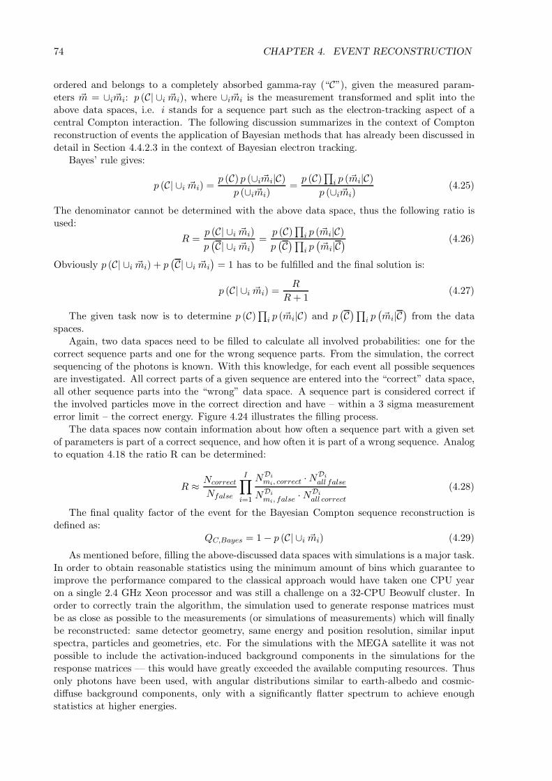
74 CHAPTER 4. EVENT RECONSTRUCTION
ordered and belongs to a completely absorbed gamma-ray (“C”), given the measured param-eters m = ∪i mi: p (C| ∪i mi), where ∪i mi is the measurement transformed and split into theabove data spaces, i.e. i stands for a sequence part such as the electron-tracking aspect of acentral Compton interaction. The following discussion summarizes in the context of Comptonreconstruction of events the application of Bayesian methods that has already been discussed indetail in Section 4.4.2.3 in the context of Bayesian electron tracking.
Bayes’ rule gives:
p (C| ∪i mi) =p (C) p (∪i mi|C)
p (∪i mi)=
p (C)∏
i p ( mi|C)p (∪i mi)
(4.25)
The denominator cannot be determined with the above data space, thus the following ratio isused:
R =p (C| ∪i mi)p(C| ∪i mi
) =p (C)
∏i p ( mi|C)
p(C)∏i p
( mi|C
) (4.26)
Obviously p (C| ∪i mi) + p(C| ∪i mi
)= 1 has to be fulfilled and the final solution is:
p (C| ∪i mi) =R
R + 1(4.27)
The given task now is to determine p (C)∏
i p ( mi|C) and p(C)∏i p
( mi|C
)from the data
spaces.Again, two data spaces need to be filled to calculate all involved probabilities: one for the
correct sequence parts and one for the wrong sequence parts. From the simulation, the correctsequencing of the photons is known. With this knowledge, for each event all possible sequencesare investigated. All correct parts of a given sequence are entered into the “correct” data space,all other sequence parts into the “wrong” data space. A sequence part is considered correct ifthe involved particles move in the correct direction and have – within a 3 sigma measurementerror limit – the correct energy. Figure 4.24 illustrates the filling process.
The data spaces now contain information about how often a sequence part with a given setof parameters is part of a correct sequence, and how often it is part of a wrong sequence. Analogto equation 4.18 the ratio R can be determined:
R ≈ Ncorrect
Nfalse
I∏i=1
NDimi, correct · NDi
all false
NDimi, false · NDi
all correct
(4.28)
The final quality factor of the event for the Bayesian Compton sequence reconstruction isdefined as:
QC,Bayes = 1 − p (C| ∪i mi) (4.29)
As mentioned before, filling the above-discussed data spaces with simulations is a major task.In order to obtain reasonable statistics using the minimum amount of bins which guarantee toimprove the performance compared to the classical approach would have taken one CPU yearon a single 2.4 GHz Xeon processor and was still a challenge on a 32-CPU Beowulf cluster. Inorder to correctly train the algorithm, the simulation used to generate response matrices mustbe as close as possible to the measurements (or simulations of measurements) which will finallybe reconstructed: same detector geometry, same energy and position resolution, similar inputspectra, particles and geometries, etc. For the simulations with the MEGA satellite it was notpossible to include the activation-induced background components in the simulations for theresponse matrices — this would have greatly exceeded the available computing resources. Thusonly photons have been used, with angular distributions similar to earth-albedo and cosmic-diffuse background components, only with a significantly flatter spectrum to achieve enoughstatistics at higher energies.

4.6. COMBINED COMPTON RECONSTRUCTION PERFORMANCE 75
Correct d�
Correct Comptonabsorption
Correct d�
Correct Photoabsorption
Correct d�
Correct Comptonabsorption
Wrong Comptonabsorption
Wrong d�Wrong Photo
absorption
Wrong d�
Correct sequence Example of a wrong sequence
Figure 4.24: Filling the Bayesian data space: For each event each possible sequence is considered. For eachsequence each part is checked whether the photon (and electron) direction is correct and whether they have —within measurement errors — the correct energy. If this is the case, the sequence part is added to the “correct”data space, otherwise to the “wrong” one. This figure illustrates which data space each sequence part belongsto: the sequence illustrated on the left is the correct one, the sequence shown on the right is one of the 23 wrongsequences. Note that the latter is only partly wrong.
The amount of simulations required to obtain a response is governed by the need to fill the“correct” data space with enough good events. Thus, due to the low efficiency and the corre-spondingly low rate of fully absorbed events of the MEGA prototype, the required computingtime for a Bayesian data space for the prototype is even higher than for the MEGA satellite.Therefore only the classical approach could be used for the prototype data analysis in Chapters7 to 9.
4.6 Combined electron tracking and Compton sequence recon-
struction performance evaluation
For real measured events, the only way to access the reconstruction performance are the ARMdistributions for the photon and electron cone, which have been introduced in Section 2.2.5. Thusthose are also used here. Correctly reconstructed and fully absorbed events contribute to thepeak of those distributions, incorrectly reconstructed events (including incompletely absorbedones) pile up off-peak.
An example of the photon ARM for both classic and Bayesian electron-track and Compton-event reconstruction can be seen in Figure 4.25. Correctly reconstructed events comprise thepeak. The distributions are plotted on a logarithmic scale to make the off-peak componentsvisible. The underlying simulation has been performed with the MEGA satellite geometry andan on-axis narrow-line 2 MeV source at infinity. Both ARMs contain all reconstructed events,regardless of sequence length, start detector (tracker or calorimeter), or if an electron trackexists — no event selections have been applied, except for a restriction to photopeak events(total energy deposit 1974–2026 keV). The white area below the thick curve corresponds to dataanalyzed with the classic algorithms (Spearman-Rank Correlation and Classic Compton sequencereconstruction) and the dark area to the same data analyzed with the Bayesian algorithms. Usingthe Bayesian algorithm reduces the number of incorrectly reconstructed events by a factor of

76 CHAPTER 4. EVENT RECONSTRUCTION
]°ARM [-150 -100 -50 0 50 100 150
coun
ts/d
egre
e
1
10
210
310
Figure 4.25: Comparison of photonARM distributions illustrating the re-construction performance of the Clas-sic (thick red line) and the Bayesianapproach (dark area). The extremebackground events which accumulatebeyond 50◦ are significantly reducedby the Bayesian approach, resulting inan overall reduction of off-ARM-peakevents by a factor of two and a corre-sponding increase in events in the ARMpeak. The simulation was performedwith 2 MeV photons (far field, on axis).All photo-peak events are used.
two, and correspondingly increases the number of events in the ARM peak. Since backgroundreduction is vital for a Compton telescope the following performance analysis will concentrateon the better approach, the Bayesian algorithms.
Figure 4.26 shows an example of the photon ARM for tracked events with an energy of 2 MeV(again far field, on axis). Besides only using photo-peak events, no event selections have beenapplied. It is obvious that the majority of these events is correctly reconstructed to within a fewdegrees. Figure 4.27 shows the electron ARM for the same events. Incorrectly reconstructedtracks accumulate at large angles (> 50◦); short tracks (2–4 interactions) constitute the majorityof these events.
Due to the long distances between interactions in the tracker and the calorimeters in MEGA,wrong short electron tracks only result in a small error (few degrees) in the direction of thescattered gamma ray eg. As a result, these events result in a broadening of the main photonARM peak rather than an increase of clearly off-peak background. The same holds for most ofthe wrong sequences inside a MEGA calorimeter. Due to the high Z of the material, multiplehits occur close together, resulting again only in a few-degree change in eg in the case of a wrongreconstruction as long as the direction of motion of the photon can still be determined correctly.As in the case for wrongly-reconstructed electron tracks, such events result in a broadening ofthe main (photon) ARM peak rather than an increase of clearly off-peak background in thedistribution.
The fact that certain classes of wrongly reconstructed events contribute to the (broadened)ARM peak rather than resulting in a clearly off-peak component makes quantifying the numberof correctly reconstructed events a non-trivial task. The method chosen first determines the“acceptance interval” around the ARM peak containing 95.5% of all events (2σ containment) —assuming perfect event reconstruction. The latter can be achieved using auxiliary informationfrom the simulation: While detector energy resolution, Doppler broadening, Moliere scattering,etc. are taken into account, the ordering of the interactions and their characterization as e.g.either close Compton interactions or electron track is taken from the simulation knowledge. Thisoptimum-case ARM is now compared to the true ARM obtained from the same data using thereal event reconstruction — i.e. without additional knowledge. The fraction of events that lieoutside the (ideal) ARM’s acceptance interval is determined for the true ARM. The differencebetween this exclusion fraction and the 4.5% excluded in the ideal case is a measure for thefraction of wrongly reconstructed events. Figures 4.28 and 4.29 illustrate the overall efficiencyof the reconstruction algorithm in terms of both photon and electron ARM. An algorithm that

4.6. COMBINED COMPTON RECONSTRUCTION PERFORMANCE 77
]°ARM - Compton cone [-150 -100 -50 0 50 100 150
coun
ts/d
egre
e
0
500
1000
1500
2000
2500
3000
]°ARM - electron cone [-150 -100 -50 0 50 100 150
coun
ts/d
egre
e
0
50
100
150
200
250
300
350
Figure 4.26: Photon ARM of tracked events with2 MeV incidence energy. Almost no wrongly recon-structed events are visible because they mainly accu-mulate in the (broadened) peak of the distribution.
Figure 4.27: Electron ARM of tracked events with2 MeV incidence energy. Wrongly reconstructedtracks result in large electron ARM values; they canbe rejected by applying the dϑ-criterion.
would achieve 2σ containment in the “acceptance interval” defined above would reconstruct allof its events correctly — so such an ideal algorithm would achieve 100% correctly reconstructedevents.
The average number of correctly reconstructed events is around 90% for tracked as well asuntracked events in the photon ARM. For not-tracked events, at higher energies the performancedecreases somewhat. This is mainly due to multiple interactions in the calorimeter — these arenot easy to reconstruct given MEGA’s energy and position resolution which lead to the largeareas of overlap in the data space as visible in Figure 4.23. The large size of the CsI bars notonly worsens the position resolution, but for events with several interactions it is also likely thatfor example in a sequence of four interactions, interaction two and three are in the same voxel.The result is a large dϕ value and a likely wrong reconstruction.
The number of correctly reconstructed events as determined via electron ARM is illustratedin Figure 4.29. As expected, the reconstruction efficiency increases with increasing photon (andthus electron) energy, from below 80% at 500 keV to above 90% for 1.5 MeV and more.
Figure 4.30 illustrates the power of one tool to reject wrongly reconstructed events, the dϑ-criterion (see Section 4.5.1.2). For 2 MeV photons and different dϑ selections, it shows how largethe excess of photons outside the original 95.5% acceptance interval of the electron ARM is. The
:5
:9
75
79
;5
;9
855
5 - $ 6
�#��!�7�8
1������!����#����&�$�
'#���0�����#��6�2�7:8
=� ,���!���� >���� ,���!����
:5
:9
75
79
;5
;9
855
5 - $ 6
�#��!�7�8
1������!����#����&�$�
'#���0�����#��6�2�7:8
=� ,���!����
Figure 4.28: Overall performance of the event recon-struction in terms of the photon ARM for various en-ergies. The average reconstruction efficiency is around90%. For a detailed explanation see text.
Figure 4.29: Overall performance of the event recon-struction as seen by the electron ARM for various en-ergies. The reconstruction efficiency increases withincreasing electron energy. For a detailed explanationsee text.

78 CHAPTER 4. EVENT RECONSTRUCTION
)-
5
-
$
6
7
85
5 85 -5 #5 $5 95 65 :5 75 ;5
$���������#�7$��8
�%�����&���$�������#��
�#��'���7:8
)-5
5
-5
$5
65
75
855
�����$�'#���������#�7:8
(? ���������� ���� ������!������� � ������!����� �����������
5
#
6
;
8-
5 5�- 5�$ 5�6 5�7 8
<1/�=�!�
�%�����&���$�������#��
�#��'���7:8
5
-9
95
:9
855
�����$�'#���������#�7:8
(? ���������� ���� ������!������� � ������!����� �����������
Figure 4.30: Effects of the dϑ event selection criterionon the fraction of events outside the acceptance inter-val of the electron ARM distribution. The ideal cut isaround dϑ = 35◦. See text for details.
Figure 4.31: Effects of using the Bayesian event re-construction quality factor as event selection criterionon the fraction of events outside the acceptance inter-val of the photon ARM distribution. The ideal cut isaround 0.95. See text for details.
overall fraction of events accepted by the dϑ-criterion is also shown. For dϑ = 180◦, when allevents are accepted, roughly 8.5% are outside the acceptance interval — in addition to the 4.5%which are expected there in the case of ideal reconstruction. Around ∼40◦, rejecting 70% of thewrongly reconstructed events (decrease from 8.5% to 2.5%) means rejecting 9% of all events,i.e. even for completely absorbed source photons more incorrectly than correctly reconstructedevents are rejected. Applying a dϑ-limit below ∼40◦ results in rejecting mainly good events.Since the dϑ-criterion is a measure of the directional quality of the electron track, such a strictdϑ-criterion results in a significantly narrower electron ARM. This reduces the fraction of (non-rejected) events outside the acceptance interval below that for an ideal reconstruction but nodϑ-cut (4.5%) — resulting in the negative values. The optimum dϑ-criterion value, which is bestempirically derived by optimizing the narrow line sensitivity of the instrument, lies between 30◦
and 40◦ in the case of the MEGA satellite instrument.Figure 4.31 illustrates a second tool to reject wrongly reconstructed events, the quality factor
derived from Bayesian event reconstruction. Some of the wrongly reconstructed events in thephoton ARM peak accumulate at large QC,Bayes values. For example, using only events withQC,Bayes ≤ 0.95 rejects 25% of the wrongly reconstructed and 10% of the correctly reconstructedevents, again using the measure of the photon ARM acceptance interval discussed above. Whilethis does not seem to be too promising (10% of valid source photons would be rejected), con-sidering the total expected background in a low-earth orbit still some advantages arise. A largeQC,Bayes value has two possible origins: Firstly, the event might be barely compatible withCompton scattering, probably because it is incompletely absorbed or does not originate froma (single) photon event. Secondly, these events might originate from data-space cells whichare heavily background dominated. In both cases the QC,Bayes is extraordinary helpful to re-ject background events. QC,Bayes is one of the main event selection criteria used to optimize aMEGA satellite’s performance (see Chapter 10).
The final proof that the event reconstruction works reliably can only be brought by a full-blown simulation and subsequent rejection of the orbital backgrounds as expected for the MEGAsatellite in low-earth orbit. This will be shown in Chapter 10.

Chapter 5
Image reconstruction for a combinedCompton and pair telescope
The effects of imperfect measurements of Compton interactions described in Section 2.2.4 leadto large ambiguities in the determination of the origin of each individual photon. The mainobjective of image reconstruction is to resolve this ambiguity and to recover the origin (sky)distribution of the photons. The leverage available to achieve this goal is the knowledge that allphotons observed reflect one common origin distribution.
5.1 Selecting an algorithm
The measurement process of any gamma-ray telescope can be described in the following way:
D( d) = T ( d;χ,ψ) × J (χ,ψ) + B( d) (5.1)
Photons emitted from a sky intensity distribution J (χ,ψ) undergo the measurement processT and, together with some background B, are measured in the data space D. The measurementprocess T completely describes the detector (absorption probabilities, etc.) as well as the physicalprocess (photo effect, Compton scattering, pair creation).
The task of image reconstruction is to invert the measurement process and to determine theimage Jrec (χ,ψ) from given measurements D( d). Since no unique solution for this inversionproblem exists, iterative approaches for the reconstruction of the image have to be chosen.
The parameters necessary to properly characterize a telescope’s imaging process are verydifferent from those optimized for the reconstruction of individual tracks or Compton events —even though each set of parameters, and thus each data space, constitutes a reduction of thesame complete data space.
For a modern tracking Compton telescope, the imaging data space D consists at least of thefollowing dimensions: the direction of the scattered gamma ray (χg, ψg), the Compton scatterangle ϕ, as well as the direction of the recoil electron (χe, ψe) and its scatter angle ε. Thetwo scatter angles have been chosen instead of the energy of the scattered gamma ray Eg andrecoil electron Ee since they constitute a description of the measurement in terms which directlyrelate to possible origin directions of a photon. For a pair telescope the minimum data spaceonly needs two dimensions, the measured energy Ei and the reconstructed origin ei. Table 5.1gives the minimum number of bins required for a measurement data space and response matrixfor the MEGA telescope in Compton mode. Reducing the number of bins further would lead tothe loss of a significant amount of information.
The required size of the imaging data space (∼ 1014 bins) and the response matrix T (∼ 1019
bins) are far beyond the possibilities of any state-of-the-art personal computer – neither can
79

80 CHAPTER 5. IMAGE RECONSTRUCTION
Size [bins]Measured parameterMEGA (Satellite) COMPTEL
Direction of scattered γ (χg, ψg) 2 · 360 × 2 · 180 360 × 180γ scatter angle ϕ 4 × 120 25Direction of recoil electron (χe, ψe) 180 × 45 1Electron scatter angle ε 90 1Sum data space ∼ 1014 1.6 · 106
Field of view (≤ 2π sr) 2 · 180 × 2 · 180 60 × 60Sum response matrix ∼ 1019 5.8 · 109
Table 5.1: Minimum size of the MEGA data space and response matrix for a sky image (far field). The numberof bins for the measured parameters is the minimum number which does not lead to the loss of a very significantamount of information. Note that the factor “2” in scattered photon direction angles and field of view correspondsto an accuracy of 0.5◦.
it be filled via simulations, nor kept in RAM for image reconstruction (the data space wouldneed ∼ 100 TB). Moreover, the proposed data space already constitutes a strong simplificationof measurements with a real modern-day Compton detector: it does not take into account thedifferent calorimeters with their different energy resolutions, it ignores multiple interactions,and it ignores the distance between the two interactions which influences the angular resolutionthrough the spatial detector resolution.
Therefore all types of imaging algorithms which use a binned data space, like they havebeen used for COMPTEL or INTEGRAL, are completely ruled out. As a consequence a list-mode based algorithm has to be used. In this type of algorithms no binned data space is used,but a mere list of events (Barrett et al., 1997). Thus the size of the data space is no longerfixed, but proportional to the number of measured events. As long as the number of events issignificantly smaller than the number of data-space bins, list-mode algorithms are preferable.For the MEGA telescope as well as for the prototype this is obviously the case. For example,during the calibration of the MEGA prototype 15 ·106 events have been measured (Andritschke,2006).
But list mode has further advantages: Since no binned data space is used, all information canbe used with full precision as it has been measured for each event. In addition to the informationcontained in the data space discussed above, for MEGA this means using the position of the firstand the second interaction of the gamma ray, the number of interactions, etc. Furthermore, it iseasy to integrate different event types like untracked Compton events, tracked Compton events,and pair events into one image. Finally, the detector geometry can easily be changed, which isespecially useful for a prototype system under construction. Nevertheless list-mode also has onedisadvantage: A pre-calculated response matrix does not exist. Instead the response has to becalculated for each event individually during image reconstruction, which is a time consumingtask depending on how accurate the response should be determined.
The selected imaging algorithm for the MEGA telescope is called List-Mode Maximum-Likelihood Expectation-Maximization (LM-ML-EM). Is has been originally developed for med-ical imaging (Wilderman et al., 1998). Its binned version is similar to Richardson-Lucy-typealgorithms (Richardson, 1972; Lucy , 1974).

5.2. THE LIST-MODE ALGORITHM 81
Sens ti ivities
list-mode data-space
(event-space)
emittingobject
1
2
23
4
1
I
j
J
bin=
voxel dimensio
n
content =emiss
ion ratej
bin =one event
content =event data d
i
3
I
mea
sure
dev
ents
unm
easu
red
even
ts(i
nfi
nit
enum
ber
)
tij
sj
i
uncovered image sp
ace
binned image sp
ace
Transition probabilities
I data space with all measured eventsI data space of all not measured eventsi event indexJ image spacej image-bin index
λ(l)j image-bin content at iteration level l
vi probability that the event i came from within the image-space (“visibility”)tij probability that a photon emitted from j is measured with the parameters of event i (“tran-
sition matrix” or “response”)
sj probability that an event emitted from j is measured (“sensitivity”): sj =PI+I tij — note
that sensitivity as used here in the context of LM-ML-EM imaging is not identical to thesensitivity of a telescope to an astrophysical source
Figure 5.1: The data spaces and their relations
5.2 The list-mode maximum-likelihood expectation-maximiza-tion algorithm
The goal of image reconstruction is to determine the origin of the photons, the image J , fromall the measurements I. The likelihood function L describes the probability that the individualmeasurements D = {yi} have been generated by the image J with the emissions λ = {λi}.
L (λ) =∏
i
p (yi, λ) (5.2)
Since the events (with a few exceptions such as decay cascades) are independent from eachother, i.e. the occurance of any event has no effect on the occurance of any other event, Poissonstatistics can be applied (with yi as the expectation of the Poisson distribution and Yi is thenumber of entries in data space bin i):
L (λ) =∏
i
p (yi, λ) =∏
i
yYii e−yi
Yi!(5.3)
or in logarithmic description:
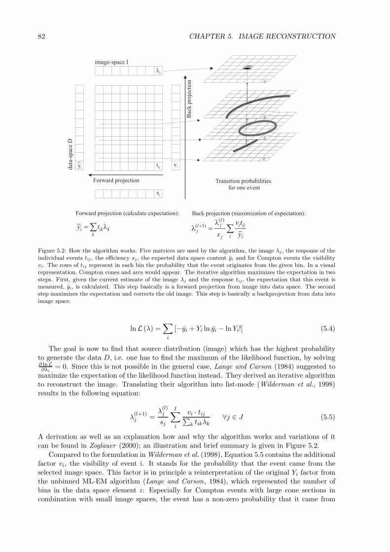
82 CHAPTER 5. IMAGE RECONSTRUCTION
image-space I
dat
a-sp
ace
D
tij
sj
viyi
j
Forward projection (calculate expectation):
�k
kiki ty ��
i i
iji
j
ljl
jy
tv
s
)(
)1(
Back projection (maximization of expectation):
Forward projection
Bac
kp
roje
ctio
n
Transition probabilitiesfor one event
j
tij
tij
tij
Figure 5.2: How the algorithm works. Five matrices are used by the algorithm, the image λj , the response of theindividual events tij , the efficiency sj , the expected data space content yi and for Compton events the visibilityvi. The rows of tij represent in each bin the probability that the event originates from the given bin. In a visualrepresentation, Compton cones and arcs would appear. The iterative algorithm maximizes the expectation in twosteps. First, given the current estimate of the image λj and the response tij , the expectation that this event ismeasured, yi, is calculated. This step basically is a forward projection from image into data space. The secondstep maximizes the expectation and corrects the old image. This step is basically a backprojection from data intoimage space.
lnL (λ) =∑
i
[−yi + Yi ln yi − ln Yi!] (5.4)
The goal is now to find that source distribution (image) which has the highest probabilityto generate the data D, i.e. one has to find the maximum of the likelihood function, by solving∂ lnL∂λi
= 0. Since this is not possible in the general case, Lange and Carson (1984) suggested tomaximize the expectation of the likelihood function instead. They derived an iterative algorithmto reconstruct the image. Translating their algorithm into list-mode (Wilderman et al., 1998)results in the following equation:
λ(l+1)j =
λ(l)j
sj
I∑i
vi · tij∑k tikλk
∀j ∈ J (5.5)
A derivation as well as an explanation how and why the algorithm works and variations of itcan be found in Zoglauer (2000); an illustration and brief summary is given in Figure 5.2.
Compared to the formulation in Wilderman et al. (1998), Equation 5.5 contains the additionalfactor vi, the visibility of event i. It stands for the probability that the event came from theselected image space. This factor is in principle a reinterpretation of the original Yi factor fromthe unbinned ML-EM algorithm (Lange and Carson, 1984), which represented the number ofbins in the data space element i: Especially for Compton events with large cone sections incombination with small image spaces, the event has a non-zero probability that it came from

5.3. IMAGING RESPONSE OF A COMPTON AND PAIR TELESCOPE 83
outside the image space. Consequently, only a fraction of the event is seen in the image, thefraction vi.
The original list-mode algorithm (Wilderman et al., 1998) did not contain any criteria tostop the iterations. It simply converges asymptotically. The best images, however, are obtainedshortly before convergence, when the width of the point sources corresponds to the intrinsicangular resolution of the detector. At this point the iteration is stopped by hand.
In the following section the determination of the response T is discussed in more detail.
5.3 Imaging response of a Compton and pair telescope
Figure 5.3: The 4 different event types of a tracking Compton and pair telescope. Left to right: UntrackedCompton events; tracked Compton events; high-energy tracked Compton events with incomplete absorption; pairevents.
Figure 5.3 illustrates the four basic event types of a MEGA-type instrument: For mostinteractions below 2 MeV, the kinetic energy of the Compton recoil electron is not sufficient toproduce a track. Therefore the photon’s origin can only be restricted to a cone (see Section2.2.4.1 and Figure 5.3, left). Its width is determined by the accuracy of energy and positionmeasurements. Between 2 and 10 MeV most events have an electron track and a reasonableamount is completely absorbed (at least in the MEGA satellite geometry). Thus, their origin isrestricted to an arc, a section of the cone (Figure 5.3, middle left), whose length is determinedby Moliere scattering. Above 10 MeV most of the Compton scatter events are incompletelyabsorbed, but the direction of electron and scattered photon is well defined. Therefore, theorigin of the photon can be restricted to the great circle between (reverse) electron and photondirection (Figure 5.3, middle right). Since the direction of the scattered gamma ray can bedetermined more accurately than the direction of the recoil electron (Moliere scattering), theorigin distribution has a drop-like shape. Measured energies can further restrict this arc (detailssee Section 2.2.4.2). The origin of pair events (Figure 5.3, right) can be calculated from electronand positron direction and energy (see Section 2.3). The main uncertainties are due to Molierescattering of electron and positron in the Silicon layers.
Two parameters describe the imaging response in Equation 5.5: the event response tij andthe sensitivity sj (Note that the word “sensitivity” denotes a quantity here that is differentfrom the sensitivity describing the overall performance of an astrophysical telescope). Figure5.4 summarizes all probabilities which contribute to these parameters for Compton events.
The easiest way to determine the sensitivity sj are Monte-Carlo simulations. This avoidsthe analytic calculation of all the probabilities of Figure 5.4. The determination of the responsetij is less straightforward: it is calculated by looping over all image-space bins and describesthe probability that the measured photon was emitted from any one given image bin. Thecalculation has two steps: determine the absorption probability and multiply by a normalizedresponse which basically represents the Compton cone/arc or pair origin distribution.
Using list mode allows to strongly simplify the large response matrix required for a binned-mode approach (see Table 5.1) — given the case of a very sparsely populated data space, as

84 CHAPTER 5. IMAGE RECONSTRUCTION
Compton scatteringprobability
Compton scatteringprocess including
Doppler-broadening
Absorptionprobabilities
Emissionprobabilities
Measurement processof scattered photon
Measurement processof recoil electron
Absorptionprobabilities
Figure 5.4: Illustration of the pro-cesses and associated probabili-ties which have to be consideredduring calculation of tij and sj ,for the case of a Compton-scatterevent.
��
p
�
l
0
0
Shape parallel tothe cone-section
Shape perpendicularto the cone-section
20-20
-2 2coneaxis
conesection
tij
scatteringplane
Figure 5.5: Modeling the mea-surement process: The cone-section is filled perpendicular toand along with two profiles: thefirst depends mainly on the en-ergy measurement and the secondon Moliere scattering.
is the case for the type of telescope discussed here. Using only the measured events as dataspace is obviously accompanied by a reduction of the size of the response matrix, since thenthe response is only needed for the measured events. The matrix is now small enough thatgenerating the tij corresponding to the measured events is feasible and drastically reduces theamount of storage space. However, since the tij have not been previously stored for all possibleevents, they have to be calculated on-the-fly. This can be done using simpler response matrices,because the matrix does not need to encode the complete Compton scattering — this informationis already contained in the event list. Knowing the properties of the Compton event yi currentlyunder consideration (scatter angle and direction, recoil electron angle and direction), the profilep (Δϕ) of the cone section and, in case of tracked events, the length l (Δν) of the arc (see Figure5.5) are sufficient to create the single-event image responses illustrated in Figure 5.2 on theright as transition probabilities for one event. The profile p of the cone-section is dominated bythe energy measurement of electron Ee and scattered gamma-ray Eg, by Doppler-broadening,and by the spatial resolution of the detector. The length l of the arc is mainly determined bydirection and energy of the recoil electron.
Two ways are used to determine the exact shape of the Compton cones and arcs. Thesimplest form uses a Gaussian approximation for p and l, with widths corresponding to the valuesderived from ARM and SPD. The more complex approach relies on predetermined responsematrices. From a large set of simulations the profiles are determined as a function of themeasured parameters: perpendicular to the cone p = p(ϕmeas
kin , Emeasi ) and perpendicular to the
scatter plane l = l(εmeaskin , Emeas
e ), where the profile represents the distribution of possible true

5.3. IMAGING RESPONSE OF A COMPTON AND PAIR TELESCOPE 85
]° [real
ϕ-meas
ϕ-150 -100 -50 0 50 100 150
]° [realν-measν
0 20 40 60 80 100 120 140 160 180
Figure 5.6: Examples of the pro-files used for reconstructing Comptonevents. The top figure shows a p pro-file for tracked events with 2 MeV mea-sured total energy and 60◦ scatter anglefor the MEGA satellite geometry. Ob-viously, the shape resembles the ARM.The wings, however, originate from in-completely absorbed events of higherenergy. The bottom figure shows thecorresponding l profile, which is mainlydetermined by Moliere scattering. It re-sembles the SPD. During image recon-struction those simulated profiles aresmoothed and interpolated.
event cones for the given measured cone, and the distribution of possible true scatter planesfor the measured scatter plane, respectively (examples are given in Figure 5.6). Figure 5.5illustrates how both factors model the Compton response. For each event the tij are calculatedby combining the event cone with the p profile perpendicular to the cone and the l shapeperpendicular to the scattering plane. The combined shape is normalized in a way that if theshape would be completely contained in the image, integrating over the image would give 1.
For low energies this response calculation gives the Compton circles/arcs of Figure 5.3,left. With increasing energy, the length of the arc gets smaller, since the Moliere scatteringdecreases, but the profile gets broader due to energy leakage. At high energies, when the energymeasurement is rather incomplete, but the direction of the recoil electron is well known, theevents have shapes like in Figure 5.3, middle right.
Compared to Compton events, pair events are trivial. The image response description relieson just one parameter to describe the angular extent of possible origins. Start point for thedetermination of the tij is the calculated origin. The applied profile is again either a 2D Gaussianfit, where the width corresponds to the angular resolution, or as a more advanced approach, usinga profile p = p(Emeas
i ), which describes the distance to the measured origin of the photon. Afuture expansion of the handling of pair events should contain not only a 1D profile, but a 2Dprofile as a function of the incidence angle, since for large incidence angles a slight shift of thereconstructed positions towards smaller incidence angles can be observed; this so called fish-eyeeffect, which has also been found in other pair telescopes like EGRET (Thompson et al., 1993),is currently not taken into account.
The performance of the image reconstruction is best demonstrated through the images ob-tained for a variety of sources. Several examples can be found in Chapters 8 and 10.
While list mode allows the most accurate description of the response within the limits ofavailable computing resources and thus probably produces the best images, it has also some dis-advantages. First, it is extremely difficult to get an absolute normalization, i.e. intensity/fluxas a result of the image reconstruction process. For this, all normalizations have to be correctlydetermined for each event. While this is no problem for 1D problems such as spectral deconvo-lution, for Compton imaging in list-mode is would be extremely time consuming. Consequently,

86 CHAPTER 5. IMAGE RECONSTRUCTION
this has not been done for any images in this work (i.e. all sj are assumed to be one, and noabsorption probabilities are calculated). Secondly, for a real space mission even only having alist of all events will require extreme computer resources. In this case (all-sky image includingall events), probably some type of simplified binned mode algorithm might be necessary.

Part III
The MEGA prototype and itsperformance
87

88

Chapter 6
The MEGA Prototype
When the completed MEGA prototype achieved its first light in February 2003 at MPE, animportant step towards the next generation of Compton telescopes was taken: MEGA addeda new dimension to the measurement of gamma rays in the Compton regime, the direction ofthe recoil electron. This chapter is dedicated to the setup and the calibration of this uniqueinstrument.
6.1 Setup of the prototype instrument
Figure 6.1: MEGA prototype detector: The tracker is housed in the central gold-colored box. It consists of 11layers; each is made up of a 3×3 array of double-sided Silicon strip detectors. The lower hemisphere of the trackeris surrounded by 20 CsI calorimeter modules, which are housed in the aluminum boxes.
Each new measurement concept, such as adding electron tracking to a Compton telescope,needs to be proven before it is applied to a full-scale gamma-ray astronomy mission. Thisvalidation involves several steps, including extensive simulations as well as the construction andcalibration of a prototype. The latter’s performance of course must be verified against thesimulations. This is the level MEGA has reached. In the future, the MEGA prototype probably
89

90 CHAPTER 6. THE MEGA PROTOTYPE
will be flown on a balloon mission to prove its background rejection capabilities. This would bean essential step before implementing an astrophysical mission.
The construction of the MEGA prototype, which started in the mid 1990s, was completedin February 2003. Since then, extensive calibration measurements have been performed. Theprototype consists of three detector sub-systems: A tracker in which the primary Comptonscatter or pair creation process takes place, a calorimeter which stops and measures all secondaryparticles, and finally, for measurements in a real astrophysical environment, an anti-coincidenceshield which encloses the detector and rejects charged particle events.
Table 6.1 summarizes the main properties of the three MEGA detectors subsystems, whichwill be described in detail in the next sections. An overview of the data acquisition system,including electronics design and trigger processing scheme, can be found in Kanbach et al.(2005) and in more detail in Andritschke (2006).
Calorimeter (one unit)Si-strip layer
2 cm 4 cm 8 cmACS
Number of units 11 8 8 4 1Material Si CsI(Tl) CsI(Tl) CsI(Tl) BC412Density [g/cm3] 2.33 4.5 4.5 4.5 1.0Active mass [g] 37.8 250 500 1,000 17,000Avg. energy res. 1σ [keV ] 9.7 @ 122 38 @ 662 38 @ 662 38 @ 662 n/aSpatial resolution [mm3] 0.47×0.47×0.5 5×5×20 5×5×40 5×5×27 (FWHM) n/aAvg. timing resolution [μs] 1 5 5 5 0.05Avg. noise threshold [keV ] 51 181 181 221 90Channels 768 120 120 240 6Avg. defective channels [%] 10 8 8 12 0
Table 6.1: Summary of the properties of the different detector sub-systems of MEGA.
6.1.1 Tracker
The most innovative part of MEGA is the tracker, also called “D1”. It has two main purposes:First, the D1 serves as scatterer or converter for the Compton and pair interactions, respectively.Second, this tracker records energy and trajectory of all generated charged particles. For eachcharged particle, the interaction position and the deposited energy in each layer of the trackeris measured with high accuracy.
These main requirements demand a tracker with a high probability for Compton scatteringor pair production, low Doppler-broadening in the case of Compton scattering, and a reasonablerange of the created electrons: The electrons need to pass through enough layers to allow a mea-surement of their direction, but they also need to be stopped within the tracker. Furthermore,a high pixelation and good energy resolution is crucial for the determination of the trajectoryand the energy of the electrons and to allow the reconstruction of the origin of the photons.Considering all requirements, Silicon-strip semiconductor detectors are the best choice for thetracker of a combined Compton and pair telescope.
The prototype tracker is a stack of eleven layers of double-sided Silicon strip detectors, whichhave a separation of 1.0 cm (Figure 6.2). Each layer consists of a 3 × 3 array of Silicon wafers(Figure 6.3). Each wafer has a sensitive area of 6 × 6 cm2, is 500 μm thick, and has a strippitch of 470 μm for a total of 128 strips per wafer side. Strips on one side of the wafer determinethe x-position of an interaction, orthogonal strips on the other side of the wafer determinethe corresponding y-position. The strips of 3 adjacent wafers in each layer are interconnected(“daisy-chained”), and the signals are read out by the front-end chips at the edge of the layer.In each layer, 3 × 128 strips are read out on each side. The tracker consists of a total activeSilicon mass of 415 g, read out by a total of 8448 channels.

6.1. SETUP OF THE PROTOTYPE INSTRUMENT 91
Figure 6.2: The complete tracker is a stack of 11layers which are spaced 1 cm from each other.
Figure 6.3: One layer of double-sided strip-detector.It has a size of roughly 23 × 23 cm2 and consists of3×3 Silicon wafers.
The achieved energy resolution varies from layer to layer and strongly depends on the tem-perature and on the quality of the individual wafers. Moreover, top and bottom sides of thewafers, called p- and n-side according to the doping required in the semiconductor, have dif-ferent properties: The energy resolution on the p-side of the strips is roughly a factor of twobetter than the resolution on the n-side. For the p-side the average FWHM at 122 keV (57Co)is 23 keV, where the best layer has 15 keV and the worst ∼30 keV for room temperature. Onaverage, the trigger threshold is 60 keV and the noise threshold 51 keV. The achieved positionresolution as measured by muons is 290 μm and the time resolution is close to 1 μs.
A detailed characterization of the strip detectors can be found in Schopper (2001) and Bloseret al. (2003). The performance of the complete tracker is described in Andritschke (2006).
6.1.2 Calorimeter
The purpose of the second detector (“D2”), the calorimeter, is to stop and measure all secondaryparticles: the electrons and positrons from pair-creation as well as the scattered Compton pho-tons. Especially for the reconstruction of Compton events, it is crucial to know the energy anddirection of the scattered gamma-ray to a very high accuracy in order to obtain well-definedevent cones. In addition, in a satellite instrument in low-earth orbit, the calorimeter also (atleast partly) shields the tracker from the dominant background component, atmospheric pho-tons. Consequently, a high stopping power is required and thus high-Z materials are preferable.In addition, the detector material must allow for a high pixelation and have a good energyresolution.
At the time the MEGA prototype was designed, the scintillator CsI(Tl) was the material ofchoice. It provides a high light yield and therefore an acceptable energy resolution, and can becut into small bars to allow a relatively high pixelation. Moreover, it is available in sufficientquantities for a reasonable price.
The MEGA calorimeter is assembled of 20 individual modules of different depth: At thebottom the blocks are 8 cm thick, the lower side walls have a depth of 4 cm and the upperside walls 2 cm. Each block consists of an array of 12 × 10 CsI crystals which have a cross-section of 5×5 mm2; their length corresponds to the block thickness. The crystals in each blockare separated by several layers of Millipore paper, which provides a high reflectivity. For lightreadout the crystals are coupled to an array of Si-PIN-diodes via Silicone cushions. The thinnerside calorimeters have PIN diodes only on the side facing away from the tracker in order tominimize the passive material between tracker and calorimeter. The large bottom calorimeters,however, do have double-sided readout. This allows the measurement of the interaction depth

92 CHAPTER 6. THE MEGA PROTOTYPE
Figure 6.4: One partially disassembled 8 cmcalorimeter module. The 120 CsI crystals surroundedby Millipore and enclosed in the Aluminum housingare visible at the top right. The removed PIN diodearray, with the Silicone cushions coupling the CsIcrystals to the diodes, is lying at the bottom left.
in the crystal, but has the disadvantage that electron/positrons moving from the tracker to thecalorimeter generate a signal in the diodes, complicating the determination of the total energyof these particles. On average, a depth resolution of 2.7 cm FWHM is reached for large energydeposits. The total active CsI mass is 10.8 kg and the calorimeters have 2880 readout channels.
The moderate energy resolution of the prototype’s calorimeter is one of the major draw-backs of the whole prototype and is the limiting factor for its angular resolution: The sidecalorimeters achieve only ∼13 % FWHM. Improvements in the performance of the calorimeterare mandatory for a final satellite version. Improving the readout from PIN to drift diodes, andprobably exchanging the scintillator material for the newer LaBr3, would allow for significantlyimproved energy resolution, lower thresholds, and shorter coincidence windows.
Detailed descriptions of the MEGA calorimeter can be found in Andritschke (2000) andAndritschke (2006).
6.1.3 Anti-coincidence shield
The third detector subsystem is the anti-coincidence shield (“ACS”). Its purpose is to allowdiscrimination against all events in the detector induced by charged particles. While this systemwas not employed during the laboratory or accelerator calibrations of the MEGA prototypediscussed below, the ACS is an intrinsic part of the whole detector system for a prototypeballoon flight and eventually for a space instrument. Charged particles of solar and cosmicorigin, as well as charged particles trapped in the earth’s magnetosphere in case of a satellite,or secondary charged particles generated in the earth’s atmosphere in the case of a balloonexperiment, are detected in the instrument along with the gamma rays of interest. Reliablerejection of charged-particle events improves the instrument’s signal-to-background ratio andlowers the demands on data acquisition and telemetry.
The MEGA ACS, built in the form of a house, almost completely encloses the detector head(see Figure 6.5). Its walls consist of 1.27 cm thick BC-412 scintillator. Embedded into thescintillator are wavelength-shifting fibers (Figure 6.6) to propagate the photons to the photomultipliers.
6.1.4 Setup of the prototype
The arrangement of the individual modules has to fulfill certain criteria: most of the scatteredgamma-rays should be stopped, and the instrument should achieve a wide field of view. Inaddition, given the relatively small number of calorimeter modules available, these should beplaced such that a minimum amount of passive material lies between the CsI and the tracker’sSilicon layers. The current setup of the prototype has been optimized using extensive simulationsto achieve the best possible sensitivity for a detection of the Crab during a future MEGA balloon
6.2. CALIBRATION MEASUREMENTS 93
Figure 6.5: The ACS dome without light shields. Figure 6.6: Wave-length shifting fibers glued into thelower ACS plate.
flight. The resulting geometry is basically a half-open sphere; in the bottom hemisphere thecalorimeters are packed as closely as possible. The distance between tracker and calorimetermodules turns out to be crucial: Putting the calorimeters too close to the tracker maximizes theefficiency, but lowers the angular resolution and thus the achievable sensitivity. The optimumdistance between bottom calorimeter and bottom layer of the tracker was determined to be5 cm — however, at the time of this calculation a significantly better energy resolution in thecalorimeters was expected than what was later achieved. The thinner calorimeter modules arearranged according to the stopping power needed for on-axis incidence of photons: small scatterangles correspond to a larger energy of the scattered gamma-ray, which need more stoppingpower. Thus the the 4 cm calorimeters where placed at the lower side, the 2 cm calorimeters atthe sides — both as close as mechanically possible to the tracker. The final setup can be seenin Figure 6.1.
6.2 Calibration measurements
The calibration of a Compton and pair telescope is a two-step process: The first step is todetermine the correlation between detector signals, which are measured in ADUs (analog-digital-converter units), and energy for each individual detector channel. Since the prototype has 11328individual channels and the response of the detector is non-linear and different for each individualchannel, the analysis of the calibration data is a lengthy process. This first step is from now onreferred to as “single-channel” calibration; details can be found in Andritschke (2006).
While in the first step the response of single detector elements to a well-defined source isestablished, the second step focuses on the response of the detector as a whole. Here, parameterssuch as overall energy resolution, angular resolution, field of view, efficiency, and polarizationand their dependence on energy, scatter-angle, etc. are determined. The evaluation of theseparameters for the MEGA prototype is discussed partly in this work and partly in Andritschke(2006). In Chapter 7, the overall energy resolution achieved with the prototype is presented.Chapters 8 and 9 discuss the angular resolution of the MEGA prototype and its capabilities asa polarimeter.
The calibration of the MEGA prototype is comprised of two phases: measurements withlaboratory sources at MPE in Garching (February to March 2003) and beam measurements atthe High Energy Gamma Source at Duke University, Durham, NC (April/May 2003).
The beam measurement was intended to explore the complete energy range of the proto-type up to 50 MeV and to determine the response of the detector to linearly polarized photons.The laboratory measurements with radioactive sources were only used for test and verification

94 CHAPTER 6. THE MEGA PROTOTYPE
Linear accelerator
Wiggler 1
Collimator
MEGA on rotatableXY-table
MirrorMirrorFree Electron Laser
Storage Ring
Wiggler 2 e-
e-
Beam-Monitor
Figure 6.7: Schematic drawing of the setup at HIGS. See text for details.
purposes before the Duke measurements. In the following, emphasis is put on the Duke measure-ments, since the initial lab measurements were taken under still changing measurement settings,and consequently no complete single-channel calibration exists. Only specific measurementsfor multiple and extended sources, which were not repeated at Duke and only require a roughcalibration, are included here.
The detailed calibration of the MEGA prototype has been performed using data acquiredwith the High Energy Gamma Source HIGS (Litvinenko et al., 1995, 1997) of the Free ElectronLaser Laboratory (FELL) at Duke University. HIGS produces 100% polarized, monoenergetic(energy spread 1-2%) gamma rays in the energy range from ∼0.7 up to ∼50 MeV via Comptonbackscattering.
A schematic of the setup of the free electron laser and MEGA can be found in Figure 6.7.The generation of gamma rays at HIGS is a two-step process: First monoenergetic photons (IR– UV) are produced by a free-electron laser. Then those photons are Compton backscatteredthrough head-on collisions with the electrons and thus reach MeV energies.
For this purpose a bunch of electrons is injected into the storage ring from a linear accelerator.A section of the ring contains wigglers, a set of magnets which generate an alternating magneticfield. The electron bunch is forced on a sinusoidal trajectory, and as a result the electronsstart emitting synchrotron radiation in the IR to UV regime — depending on electron energyand wiggler parameters. The forward component is captured in a laser cavity, which is formedby two mirrors at the beginning and end of the wiggler-section of the storage ring. All beamand wiggler parameters are chosen such that electron and photon bunch are moving throughthe wigglers simultaneously. For certain resonance energies of the electrons, they interact withthe electric field of the previously generated photons. As a result the electrons emit in phase,which leads to resonant amplification of the photon bunch — the free-electron laser, producingmonoenergetic and 100% polarized photons.
When the facility is not only used as a free electron laser, but as a gamma-ray source as duringthe MEGA calibration, a second electron bunch is injected in the storage ring. This bunch isstretched compared to the first one, to prevent stimulated emission (lasing). It hits the photonbunch head-on in the field-free zone between the wigglers. The photons are inverse-Comptonscattered on the electrons and boosted to gamma-ray energies. During the backscattering processof low energy photons with high energy electrons, the original polarization is almost 100%conserved (Park et al., 2001) — this is not to be confused with the distribution of photonscatter directions described by the Klein-Nishina Equation 2.11. Lead collimators, which arelocated ∼60 m from the collision area, select the backscattering component of the beam, whichthen interacts in the MEGA detector. The opening angle of the collimator determines the energy

6.2. CALIBRATION MEASUREMENTS 95
1
2
3
4
567
Figure 6.8: Setup of MEGA at Duke: The MEGA prototype (1) is located below a Styrofoam housing to regulatethe temperature via an air-conditioning system (4). MEGA is mounted on an XY-table (2) to scan the detectorwith the narrow pencil beam. To verify the field of view,, the whole XY-table assembly can be rotated (3) aroundthe center of the tracker. The data acquisition system (front-end (5), ADCs (6), CPU (7)) is also shown.
spread and the beam width. For the MEGA calibrations the latter was either 0.5 or 1 inch (1.27or 2.54 cm), corresponding to an energy spread of roughly 1-2%. To record the intensity of thebeam as a function of time, between MEGA and the collimator a beam monitor was installed.A detailed description of the beam monitor can be found in Andritschke (2006).
Figure 6.8 illustrates the MEGA setup. The detector was mounted on an XY-table, whichallowed to illuminate different positions of the MEGA tracker with the gamma-ray pencil beam.Eleven positions were illuminated: the centers of all nine wafers, the electronics and the calorime-ter. The latter two measurements were intended to verify the background rejection capabilities.To scan the detector at different incidence angles and determine the field of view of the detector,the XY-table was mounted rotatable around the center of the tracker.
The original calibration plan was to cover the whole beam energy range from 0.7 to 50 MeVwith at least 7 data points (710 keV, 2 MeV, 5 MeV, 8 MeV, 12 MeV, 25 MeV and 50 MeV)and to sample the field of view — at least for energies not accessible with laboratory radioactivesources (5 MeV and higher) — with at least four angles: 0◦, 30◦, 60◦, and at least one incidenceat 180◦ to determine the background rejection capability of the event reconstruction algorithms.The calibration schedule was divided into two sections, up to 8 MeV and above 8 MeV, due to anecessary change of mirrors for higher energies which took 72 h and had to be performed duringthe weekend. Unfortunately, at lower energies the beam flux achieved was significantly lower

96 CHAPTER 6. THE MEGA PROTOTYPE
Energy [MeV] 0.7 2 5 8 10 11.9 17 25 37 490◦ 270 216 315 225 405 405 405 315 405 103530◦ 216 0 315 0 495 495 495 360 450 36060◦ 0 0 450 0 540 675 540 540 540 54080◦ 0 0 0 0 0 350 0 540 450 450120◦ 0 0 90 0 0 135 0 90 90 135180◦ 0 0 90 0 135 90 0 0 90 90
Table 6.2: Matrix of all measurements as a function of energy and incidence angle. Table entries representthousands of triggered events recorded in a given configuration.
than expected so that significantly more time per energy and incidence direction was necessary toachieve the minimum number of photons. In addition, the beam showed stronger contaminationthan expected, so that only the minimum requirements were achieved below 10 MeV. At higherenergies, the beam flux was significantly higher, and an unexpected time extension was granted.As a result, at energies above 8 MeV MEGA recorded significantly more events at more anglesand energies than were required to determine the energy, angular and polarization response ofthe prototype.
A complete list of measurements performed, as well as the number of triggered eventsrecorded in each run, is given in Table 6.2. These number, however, are not equal to the numberof valid photon events detected, as later chapters will show. The following three chapters arededicated to the analysis of different aspects of this data.

Chapter 7
Event characteristics and spectralproperties of the MEGA prototype
This and the following two chapters describe the recovery of the three main photon propertiesfrom MEGA prototype calibrations: energy, direction, and polarization. Note that these chap-ters are not intended to fully characterize the prototype, instead they focus on the recovery ofthe original photon parameters from and the performance of the reconstruction and imagingalgorithms on real data. Other key parameters of the prototype such as efficiency, etc. are dis-cussed in Andritschke (2006). This chapter is based exclusively on the on-axis beam-calibrationdata from the Duke campaign, for which the finest sampling of the spectral domain is available.
7.1 Event statistics
Compared to the event reconstruction of the MEGA satellite geometry — which thus far existsin simulations only, the actual prototype provides a variety of challenges: Non working channels,channels providing fake signals, high and varying thresholds, capricious energy resolutions aswell as position resolutions in the large bottom calorimeters, etc. Moreover, the relatively smallprototype with its large amount of passive material is severely handicapped by incomplete energymeasurements.
For the event reconstruction, the classic approach has been used (Spearman-Rank correlationfor tracking, Classic Compton Sequence reconstruction for the Compton interactions), becausethe Bayesian approach would have required more CPU resources than available. The eventreconstruction as described in Chapter 4 did not use any prior knowledge about the inputphotons, such as their energy or the path of the beam within the prototype. This event statisticsis intended to provide an overview of the characteristics of the data. Thus no event selectionshave been applied except where explicitly noted, and wrongly reconstructed events are part ofthe data set.
Figure 7.1 shows the distribution of the different event types as a function of the incidentphoton energy. According to their cross-sections (see Figure 1.1), the fraction of Compton eventsis expected to decrease with increasing energy, while the number of pair events should increase.Contrary to this expectation, especially at 710 keV a high fraction of pair and charged-particle(e.g. single straight paths from the tracker into the calorimeter or showers) events has beendetected. Since such events could not possibly have been induced by 710 keV photons, thisindicates a significant contamination of the beam with high energy photons.
This can easily been shown by imaging these events. Figure 7.2 prove that the pair-producingphotons originate from the beam. Direct energy measurements at tens of MeV are not possiblewith the small prototype (see next section), but the achieved angular resolution and the opening
97
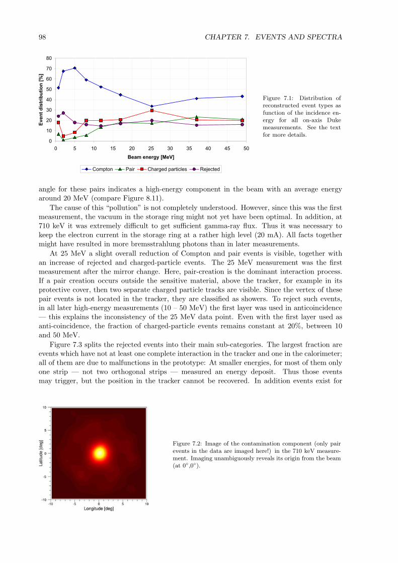
98 CHAPTER 7. EVENTS AND SPECTRA
5
85
-5
#5
$5
95
65
:5
75
5 9 85 89 -5 -9 #5 #9 $5 $9 95
=� �#��!�7�8
�'#��$������&���#�7:8
������� .�� ���������� ��� <�@� ���
Figure 7.1: Distribution ofreconstructed event types asfunction of the incidence en-ergy for all on-axis Dukemeasurements. See the textfor more details.
angle for these pairs indicates a high-energy component in the beam with an average energyaround 20 MeV (compare Figure 8.11).
The cause of this “pollution” is not completely understood. However, since this was the firstmeasurement, the vacuum in the storage ring might not yet have been optimal. In addition, at710 keV it was extremely difficult to get sufficient gamma-ray flux. Thus it was necessary tokeep the electron current in the storage ring at a rather high level (20 mA). All facts togethermight have resulted in more bremsstrahlung photons than in later measurements.
At 25 MeV a slight overall reduction of Compton and pair events is visible, together withan increase of rejected and charged-particle events. The 25 MeV measurement was the firstmeasurement after the mirror change. Here, pair-creation is the dominant interaction process.If a pair creation occurs outside the sensitive material, above the tracker, for example in itsprotective cover, then two separate charged particle tracks are visible. Since the vertex of thesepair events is not located in the tracker, they are classified as showers. To reject such events,in all later high-energy measurements (10 – 50 MeV) the first layer was used in anticoincidence— this explains the inconsistency of the 25 MeV data point. Even with the first layer used asanti-coincidence, the fraction of charged-particle events remains constant at 20%, between 10and 50 MeV.
Figure 7.3 splits the rejected events into their main sub-categories. The largest fraction areevents which have not at least one complete interaction in the tracker and one in the calorimeter;all of them are due to malfunctions in the prototype: At smaller energies, for most of them onlyone strip — not two orthogonal strips — measured an energy deposit. Thus those eventsmay trigger, but the position in the tracker cannot be recovered. In addition events exist for
Figure 7.2: Image of the contamination component (only pairevents in the data are imaged here!) in the 710 keV measure-ment. Imaging unambiguously reveals its origin from the beam(at 0◦,0◦).

7.1. EVENT STATISTICS 99
5
85
-5
#5
$5
95
65
:5
75
;5
855
5 9 85 89 -5 -9 #5 #9 $5 $9 95
=� �#��!�7�8
�'#��$������&���#�7:8
>���������� �������������8��������-
=�������������"<
A�!���,������ �
Figure 7.3: Rejection reasons forevents during the event reconstruc-tion (100% = all rejected events).A detailed description can be foundin the text.
5
85
-5
#5
$5
95
65
:5
75
;5
855
5 9 85 89 -5 -9 #5 #9 $5 $9 95
=� �#��!�7�8
*��#���������������#$�#��������$�
'#���7:8
>���� ,�� =� ,��
Figure 7.4: Distribution of trackedand not tracked events as a func-tion of energy (100% = all Comp-ton events). The large fraction ofnot tracked events at higher ener-gies originates from photons whichhave their first interaction in thecalorimeter and a secondary parti-cle interacting in the tracker.
which the trigger hardware was influenced by electrical inference, resulting in events which haveonly hits in the tracker or only hits in the calorimeter. The second category are events where nosequence of the recorded interactions is compatible with Compton kinematics. The final rejectioncategory are events with too many individual hits. Since Compton sequence reconstruction is analgorithm of order O (n!) (Section 4.5.2), computational demands become too high if the numberof individual interactions exceeds a certain threshold. This cut-off is set to seven interactions(using the definition of Chapter 4.5), i.e. an electron track is counted as one interaction).
Figure 7.4 shows the break-down of Compton events into events with and without track,restricted to events which the algorithm determined to have started in the tracker. Up to5 MeV, the fraction of tracked events increases as expected. However, then the trend reversesand the fraction of untracked events increases again. Simulations show that almost all of theseCompton events without track above 5 MeV truly had their first interaction in the calorimeterbefore some secondary produces a hit in the tracker. They typically have one hit in D1 andone cluster in D2 and are incompletely absorbed. They fall in the “two interactions withouttrack” category of Chapter 4.5.1.1 for which no good rejection possibility exists in the contextof Classic event reconstruction. Given the simulation-based knowledge that they are mostlywrongly reconstructed events, this class of events is not included in the subsequent analysis.
Figure 7.5 illustrates the average track and Compton sequence length. Up to 8 MeV theaverage track length increases, then it deceases again. The explanation for the decrease athigher energies are again wrongly reconstructed and incompletely absorbed events. However,these wrongly reconstructed events with tracks can be nicely rejected using the dϑ-criterion fromSection 4.5.1.2. As expected, the average number of (separable) Compton interactions increaseswith the total energy.

100 CHAPTER 7. EVENTS AND SPECTRA
5�5
5�9
8�5
8�9
-�5
-�9
#�5
#�9
$�5
$�9
9�5
5 9 85 89 -5 -9 #5 #9 $5 $9 95
=� �#��!�7�8
�'����#�����#��#�������#�
�!������� ,�������� ,���!��������
�!��������� ���������� �������
Figure 7.5: Average Comp-ton track length and averageCompton sequence lengthas a function of energy.In contrast to expectations,above 8 MeV the tracklength decreases with in-creasing energy. The rea-son are events which interactin the calorimeter first andthen a bremsstrahlung pho-ton produces a track. Theycan easily be rejected by thedϑ-criterion.
7.2 Spectral response
One important task of a telescope is to measure the energy of the detected photons. In thisrespect, the Compton regime presents an extraordinary challenge, since the photons have theleast probability to interact (see cross-sections Figure 1.1), and if they interact via Comptonscattering, the scattered photon nevertheless might escape the detector.
Figure 7.6 shows the measured spectra after the event reconstruction for five different on-axismeasurements. The left image shows all events (no event selections have been applied), the rightimage shows only events for which the minimum distance between cone and origin (i.e. incidentbeam direction) is less than 10◦.
Only at 710 keV the MEGA prototype has sufficient active mass to stop enough photonscompletely to generate a photo peak despite the mediocre energy resolution of the prototype.For this beam energy the combined energy resolution of the prototype is (41±4) keV (one sigma).At 2 MeV, the suboptimal energy resolution smears out a possible photo peak. At even higherenergies, the total energy cannot be measured: If the photon interacts via Compton scattering,the scattered photon probably escapes. If the photon interacts via pair creation, likely most ofthe energy is deposited in passive material; moreover, if the electron or positron does hit theCsI, the energy deposited is high enough to lie in a domain for which no calibration for thecrystals exists — as a result, the recovered energy is most likely wrong.
Again, the term “incompletely absorbed events”, as used in this work, refers to all photoninteractions which fulfilled the instrument’s trigger criteria but where the photon’s energy couldnot be retained in the active material of the detectors — be it that particles escape from thedetector, that energy is deposited in passive material or dead voxels, or that an energy depositis below the relevant detection threshold.
Reproducing these measured spectra in simulations is a daunting task, because too manyproperties of the individual detectors are not well known.
• One set of problems arises from the instability of the system: Thresholds and energyresolutions vary with time and temperature. Only the time-averaged system properties areroughly known, and corresponding (large) uncertainties are introduced into the simulation.To include for example the noise threshold in the simulation, the overall distribution ofthe thresholds is determined for all channels of e.g. the tracker and fitted by a Gaussian.During simulation a random threshold is determined for each individual hit, given the mean

7.2. SPECTRAL RESPONSE 101
710 keV
Energy [keV]0 100 200 300 400 500 600 700 800 900 1000
coun
ts/k
eV0
20
40
60
80
100
120
140
Energy [keV]0 100 200 300 400 500 600 700 800 900 1000
coun
ts/k
eV
0
20
40
60
80
100
2 MeV
Energy [keV]0 500 1000 1500 2000 2500
coun
ts/k
eV
0
20
40
60
80
100
120
140
160
Energy [keV]0 500 1000 1500 2000 2500
coun
ts/k
eV
0
10
20
30
40
50
60
70
80
90
8 MeV
Energy [keV]0 1000 2000 3000 4000 5000 6000 7000 8000 9000 10000
coun
ts/k
eV
0
2
4
6
8
10
12
14
16
18
20
Energy [keV]0 1000 2000 3000 4000 5000 6000 7000 8000 9000 10000
coun
ts/k
eV
0
1
2
3
4
5
6
7
17 MeV
Energy [keV]0 2000 4000 6000 8000 10000 12000 14000 16000 18000 20000
coun
ts/k
eV
0
2
4
6
8
10
12
14
16
18
20
Energy [keV]0 2000 4000 6000 8000 10000 12000 14000 16000 18000 20000
coun
ts/k
eV
0
2
4
6
8
10
50 MeV
Energy [keV]0 10000 20000 30000 40000 50000 60000
coun
ts/k
eV
0
1
2
3
4
5
Energy [keV]0 10000 20000 30000 40000 50000 60000
coun
ts/k
eV
0
0.5
1
1.5
2
2.5
3
Figure 7.6: Measured spectra after the event reconstruction: Left, the spectra are shown without selections;on the right side only those events are selected which originate from the beam direction (radius: 10◦). TheMEGA prototype is only at 710 keV capable to completely stop the majority of its events. All other energies aredominated by incompletely absorbed events.

102 CHAPTER 7. EVENTS AND SPECTRA
and the sigma of the Gaussian fit. The same procedure is applied to all other detectorproperties.
However, most system properties were determined in the dedicated “single-channel” cal-ibrations and constitute short-term snapshots of the instrument relative to the 2-weekcalibration campaign; each parameter may have varied more widely over the whole timespan. In addition, variations of individual system properties, such as thresholds or gainsin different channels, may well be correlated. The simulation, however, for lack of moredetailed information must assume that each parameter such as threshold, measured en-ergy, etc. varies according to a certain distribution and independent of variations in othermeasured quantities for a given event.
• The energy calibration of the tracker is also problematic: The highest energy calibrationsource, which was available at Duke, was 57Co with its 122 keV line. However, the meanenergy deposit of an electron passing through one tracker layer is Landau-distributed witha mean value around 200 keV and a very long tail. Consequently, no calibration for themean energy deposit exists! The low-energy calibration of the tracker is extrapolatedto higher energies. Thus comparing the measured energy deposit with the simulated onesreveals certain differences: The peak energy of the measured Landau distribution is roughly15% lower than that of the simulated distribution, but the measured distribution has asignificantly stronger high-energy tail. Overall, this results in a roughly 7% higher averagedeposited energy for the 2 MeV measurement compared to the simulation. The reasonis probably non-linearities in the electronics which cannot be adequately calibrated giventhe available source calibration data.
• A similar problem exists for the calorimeter. It was not possible to calibrate the detectorwith sources below 511 keV, because no suitably strong sources were available at Duke.This is a problem because higher-energy photons can interact deep in the calorimeter, de-positing — in a Compton interaction — less than 511 keV in one CsI crystal. Furthermore,the highest-energy calibration (1275 keV of 22Na) was rather difficult to evaluate; in partic-ular a calibration was not possible for all channels (Andritschke, 2006). Charged particles,such as the electrons from e.g. 25 MeV and higher photons, can deposit several MeVs inone crystal. Again, for such events an extrapolation of the low-energy calibration had tobe used.
• Another problem arises from the trigger threshold in combination with the coincidencewindow. To reduce the amount of chance coincidences, the trigger signals of tracker andcalorimeter must be detected within a 2.2 μs time window. Unfortunately, CsI calorimetershave a slow response, i.e. for weak signals the threshold level might have not been reachedbefore the end of the coincidence window. For low-energy events, this effect introduces anadditional threshold to the one set by the hardware, and is expected to raise the hardwarethreshold by roughly 100 keV.
• A final problem arises from the differences between the calibration and measurement mode.In calorimeter-calibration mode, the front-end chip holds the signal a certain time afterthe trigger has been raised. In measurement mode, the signals of the calorimeters areheld a certain time after the tracker has triggered. This results in two problems: Alarger D1 signal generates a trigger signal faster than a small one, varying the triggertime and thus the height of the calorimeter signal at the time the signal is held. Thesecond problem is that the delay between D1 trigger and D2 readout is fixed; the delaytime has been optimized for the 662 keV measurement. Just how accurately the single-channel calibration obtained in calibration mode reflects the behavior of the instrument in

7.2. SPECTRAL RESPONSE 103
measurement mode for other photon energies remains unknown. The fixed-delay readout,however, is expected to introduce some additional energy measurement uncertainty in thecalorimeters.
The 2 MeV Duke measurement is least influenced by the problems detailed above and thusis best suited for a comparison between measurements and simulations: the measured events —at least those close to the “photo-peak” — are above all trigger threshold effects, and the totalenergy at least of the calorimeter hits is mostly within the calibration range. Figure 7.7 shows theinfluence of the different detrimental effects on the 2 MeV spectrum. The first figure shows theideal beam spectrum, which has an intrinsic width of roughly 1%. In the next step all geometricaleffects are activated: photons/electrons escape from the detector or deposit energy in passivematerial. The majority of all events (82%) are incompletely absorbed. Technically, one wouldhave to consider all tracked events in the MEGA prototype to be incompletely absorbed events:The electron loses energy in the air between the layers of the tracker; this shifts the photopeakslightly to lower energies. The third spectrum includes the effects of thresholds (noise as wellas trigger) and not-working channels of the active material. The total number of photo peakevents is reduced to 7%. In the final step, the MEGA prototype’s energy resolution is appliedto the simulated data — and completely smears out the photo peak. Although several details ofthe detector’s behavior remain unaccounted for in the simulation — as discussed above — thefinal simulated spectrum resembles the measured one (thick line) quite nicely.
Figure 7.8 shows where the energy is lost. On average, for the 2 MeV measurement for eachtriggered event 2/3 of the incident photon’s energy is detected. 19% is lost in passive material,9% is carried away by escaping particles, and on average 5% is not recorded due to thresholdeffects.
The spectral resolution of the MEGA prototype is significantly below the performance neededfor a space mission. In addition, several of the detector’s shortcomings are hard to correctlycalibrate and consequently cannot be fully incorporated into a simulation of the detector. Thusthe following recommendations have to be made for future developments:
• The single most important improvement recommendation concerns the calorimeters andits electronics, to improve the energy resolution and the stability of the prototype as wellas to lower its thresholds.
• Additionally, the calorimeter needs to completely enclose the tracker and be as compactas possible, in order to significantly reduce the number of escaped photons.
• Furthermore, the amount of passive mass needs to be minimized, especially between trackerand calorimeter.
• Finally, the tracker must be large enough to accommodate even high-energy tracks in theCompton regime. Assuming that at least 14 MeV photons have to be stopped (at thisenergy Compton and pair cross-section have equal energies), assuming that 50% of theenergy is transfered to the electron and that on average 200 keV are deposited per layer,around 35 layers are necessary to stop this electron. Consequently, a significantly largertracker is necessary. Alternatively, the tracker might be enclosed by thicker Silicon layersat the bottom and the sides (or even Germanium or CZT).
Given the current spectral response of the MEGA prototype with its strong energy dispersionabove ∼1 MeV where no photo-effect is visible, the original spectral information can only be

104 CHAPTER 7. EVENTS AND SPECTRA
Energy [keV]0 500 1000 1500 2000 2500
coun
ts/k
eV
0
1000
2000
3000
4000
5000
6000
7000
8000
(A) Incident beam spectrum of the 2 MeV Duke measure-
ment with a 1% energy resolution of the beam itself. Only
events are shown which in the simulation interact in both
D1 and D2 detector material.
Energy [keV]0 500 1000 1500 2000 2500
coun
ts/k
eV
0
100
200
300
400
500
600
700
800
900(B) Reconstructed beam spectrum using an idealized de-
tector. Energy resolution (and correspondingly calorime-
ter depth resolution) is assumed perfect, and all thresh-
olds are assumed at 0 keV. However, escaping photons and
electrons as well as deposits in passive material are con-
sidered. The Compton edge, backscatter peak, and first
escape peak are clearly visible. The photo peak is slightly
shifted towards smaller energies, due to the energy loss of
electrons in air while traveling from layer to layer.
Energy [keV]0 500 1000 1500 2000 2500
coun
ts/k
eV
0
20
40
60
80
100
120
140
160
180
200
(C) Reconstructed beam spectrum including losses induced
by trigger and noise thresholds as well as not working pix-
els/strips strongly reduces the photo-peak as well as the
total number of detected events.
Energy [keV]0 500 1000 1500 2000 2500
coun
ts/k
eV
0
20
40
60
80
100
120
140
160 (D) Final reconstructed beam spectrum. Adding the
appropriate energy resolution completely smears out the
photo peak. Although there are still several uncertainties
in the simulation (see text for details on detector properties
that cannot be incorporated), the final simulated spectrum
resembles the shape of the measurement (thick line, nor-
malized to same total number of counts in the spectrum)
quite closely.
Figure 7.7: The effects of the measurement process on the simulated 2 MeV spectrum. (A)-(D) show the increasingenergy dispersion due to the measurement process and the instrumental function.
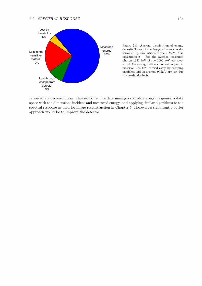
7.2. SPECTRAL RESPONSE 105
3������
������
6:B
+����������
�� ������
���� ���
;B
+��������
�������!�
������
8;B
+���&�
����������
9B
Figure 7.8: Average distribution of energydeposits/losses of the triggered events as de-termined by simulations of the 2 MeV Dukemeasurement. For the average measuredphoton 1342 keV of the 2000 keV are mea-sured. On average 380 keV are lost in passivematerial, 185 keV carried away by escapingparticles, and on average 90 keV are lost dueto threshold effects.
retrieved via deconvolution. This would require determining a complete energy response, a dataspace with the dimensions incident and measured energy, and applying similar algorithms to thespectral response as used for image reconstruction in Chapter 5. However, a significantly betterapproach would be to improve the detector.

106 CHAPTER 7. EVENTS AND SPECTRA
Chapter 8
Imaging properties of the MEGAprototype
One key functionality of a telescope is its ability to retrieve the origin of the measured photons.For telescope designs that do not directly yield a sky image, but instead require reconstruction,two sets of properties need to be examined: the quality of information contained in individualevents, discussed in the first part of this Chapter, and the accuracy with which the imaging al-gorithm can retrieve input sky (or laboratory source) distributions from the data. For a trackingCompton telescope two parameters are critical for its imaging performance: the accuracy withwhich the width and the length of the arcs of the Compton cone can be determined — thesedetermine the size of the point-spread function of the telescope. For a pair telescope’s imagingperformance, the critical parameter is the direction accuracy of each photon’s point of origin asdetermined from the electron’s and positron’s tracks (and energies). In the second part of thisChapter, the LM-ML-EM-Algorithm described in Chapter 5 is applied to laboratory and beamdata of the MEGA prototype to evaluate the full imaging system’s response to point sourceson and off axis as well as to illustrate its response to multiple sources and extended emissionregions.
8.1 Angular resolution
8.1.1 The Compton regime
The size of the point-spread function, and thus the angular resolution of a tracking Comptontelescope, is determined by the shape of the arcs of the Compton cones. As described in Chapter5, this shape can be described by two parameters: the width of the arc (ARM), which is mainlydetermined by the energy and position measurements, and of course influenced by Doppler-broadening, and the length of the arc (SPD), which is determined by the accuracy with whichthe direction of the recoil electron track can be measured.
8.1.1.1 Width of the Compton cone
The width of the Compton cones and arcs is measured by the Angular Resolution Measure(ARM) as defined in Section 2.2.5. It is a complex function of several parameters of Comptonscattering such as scatter angle and total energy, but also background suppression cuts like thosedetailed in Chapter 4 (cuts on the quality factor of the electron track, of the Compton sequence,and of course the dϑ-criterion). The ARM distributions shown here have been obtained fromMEGA beam measurements using the following event selections:
107

108 CHAPTER 8. IMAGING PROPERTIES OF THE MEGA PROTOTYPE
710 keV
]°ARM - Compton cone [-30 -20 -10 0 10 20 30
coun
ts
0
20
40
60
80
100
120
140
160
180
200
Figure 8.1: Right column: ARMs of trackedevents from 2 to 8 MeV: At 2 MeV the ARMis dominated by the energy resolution in thecalorimeters; contributions from the other ef-fects (position resolutions, energy resolutionin the tracker) are a factor of three smaller(compare Table 8.1). At higher energies theangular resolution improves. The fits, con-sisting of a combination of Lorentz aus Gaussfunctions, are only used to determine theFWHM of the distribution.
2 MeV
]°ARM - Compton cone [-30 -20 -10 0 10 20 30
coun
ts
0
50
100
150
200
250
]°ARM - Compton cone [-30 -20 -10 0 10 20 30
coun
ts
0
50
100
150
200
250
5 MeV
Figure 8.2: Left column: ARMs of nottracked events at 710 keV to 2 MeV. While at710 keV the angular resolution is dominatedby energy resolutions, at 2 MeV the contri-bution of energy and position resolution arerather similar.
]°ARM - Compton cone [-30 -20 -10 0 10 20 30
coun
ts
0
20
40
60
80
100
8 MeV .
]°ARM - Compton cone [-30 -20 -10 0 10 20 30
coun
ts
0
5
10
15
20
25
30
35
• The event has to pass the event reconstruction as a kinematically correct Compton event,which can be uniquely identified as moving from tracker to calorimeter. Ambiguous two-site events without track (Section 4.5.1.1) have been rejected.
• Due to the lack of a photo peak above 710 keV, an energy window of ±5% around theknown source energy has been applied. For comparison, the energy resolution (one sigma)of the beam was 1-2%.

8.1. ANGULAR RESOLUTION 109
• The Compton scatter angle ϕ has to be larger than 7◦ and smaller than 90◦. Both cutseliminate wrong Compton events — eliminating small-angle scatters avoids second inter-actions close to the beam path, and true backscattering is very unlikely given the detectorgeometry.
• Only events were used whose reconstructed start point is consistent with the beam path.This eliminates background, but has no effect on the angular resolution.
Since the background can be rejected sufficiently well by only using events first interacting inthe beam path, no additional background rejection cuts, such as cuts on the quality factor ofthe reconstruction or on the dϑ-criterion, are necessary. Reasonable cuts here would not have asignificant influence on the angular resolution of the MEGA prototype; they would only rejectsignificantly wrong reconstructed events.
Figures 8.1 and 8.2 show the ARM for the 0.71, 2, 5 and 8 MeV measurements at Duke.The left column shows not-tracked events, the right column tracked events. Ignoring the 8 MeVmeasurement for the moment, the angular resolution improves with increasing energy. Thisis expected, because at higher energies the relative energy measurement uncertainties decreaseand along with a smaller average Compton scatter angle the angular resolution improves (detailssee Section 2.2.5) — as long as the photon is completely absorbed and correctly reconstructed.Similar arguments hold for the difference between tracked and not tracked events at 2 MeV: Inorder to generate an electron track, a sufficient amount of energy needs to be transferred to theelectron. This results in large Compton scatter angles, where energy measurement uncertainties,especially those of the calorimeters, have a larger influence on the angular resolution than atsmall Compton scatter angles (Figure 2.15).
While the ARM distributions up to 5 MeV are smooth functions, MEGA’s ARM distributionat 8 MeV has a peculiar shape: It has a strong central peak and then the distribution broadensabruptly. It turns out that the peak corresponds to two-site events with track, and the broad dis-tribution to multiple Compton interactions (details see Chapter 4.5.1.3) with several interactionsin the same calorimeter module. While the track defines the start of the sequence rather nicely,the lack of a good energy calibration at high energies in combination with a very moderate posi-tion resolution makes it difficult to find the correct sequence, particularly if several interactionsoccur in close proximity. Simulations have shown that in order to reliably distinguish betweendifferent possible Compton interaction sequences in the case of multiple interactions in a singlecalorimeter module, energy resolutions of a few percent at most, not ∼13% as in the prototypeare required. Similarly, position resolutions corresponding to geometrical Compton scatter an-gles of several degrees, and not a few tens of degrees, are necessary. Another reconstructionapproach would be to use the energy-weighted center of interaction in a calorimeter module incase of multiple hits. However, in the energy regime under consideration, the distances betweeninteractions are large enough that no improvement is possible.
Figure 8.3 summarizes the achieved angular resolution. The left figure includes all eventswhich comply with the above event selections, the right figure only two-site events. As explainedabove, two-site events are expected to give a better resolution than multiple events, given theperformance characteristics of the MEGA prototype. Overall, in terms of angular resolutionbelow 10 MeV, the prototype has a hard time competing with COMPTEL (smooth line in thefigures). Since it is possible to build an improved calorimeter, the satellite instrument will havea significantly better angular resolution (Figure 10.5).
Reconstructing the origin of Compton events requires knowledge of interaction positions aswell as deposited energies. Thus the angular resolution is influenced by most of the imperfec-tions of the prototype, with contributions from energy and position resolutions, thresholds, aswell as non-linearities and time-variabilities. Table 8.1 illustrates how activating the individualimperfections in the simulation, one after the other, influences the final angular resolution of
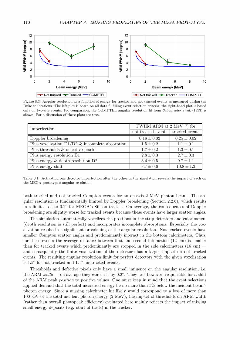
110 CHAPTER 8. IMAGING PROPERTIES OF THE MEGA PROTOTYPE
5
-
$
6
7
85
8-
5 - $ 6 7 85
=� �#��!�7�8
�6��9>3��7$��8
>���� ,�� =� ,�� �%3.=(+
5
-
$
6
7
85
8-
5 - $ 6 7 85
=� �#��!�7�8
�6��9>3��7$��8
>���� ,�� =� ,�� �%3.=(+
Figure 8.3: Angular resolution as a function of energy for tracked and not tracked events as measured during theDuke calibrations. The left plot is based on all data fulfilling event selection criteria, the right-hand plot is basedonly on two-site events. For comparison, the COMPTEL angular resolution fit from Schonfelder et al. (1993) isshown. For a discussion of these plots see text.
FWHM ARM at 2 MeV [◦] forImperfectionnot tracked events tracked events
Doppler broadening 0.18 ± 0.02 0.25 ± 0.02Plus voxelization D1/D2 & incomplete absorption 1.5 ± 0.2 1.1 ± 0.1Plus thresholds & defective pixels 1.7 ± 0.2 1.3 ± 0.1Plus energy resolution D1 2.8 ± 0.3 2.7 ± 0.3Plus energy & depth resolution D2 3.4 ± 0.5 9.7 ± 1.1Plus energy shift 3.7 ± 0.6 10.8 ± 1.3
Table 8.1: Activating one detector imperfection after the other in the simulation reveals the impact of each onthe MEGA prototype’s angular resolution.
both tracked and not tracked Compton events for an on-axis 2 MeV photon beam. The an-gular resolution is fundamentally limited by Doppler broadening (Section 2.2.6), which resultsin a limit close to 0.2◦ for MEGA’s Silicon tracker. On average, the consequences of Dopplerbroadening are slightly worse for tracked events because these events have larger scatter angles.
The simulation automatically voxelizes the positions in the strip detectors and calorimeters(depth resolution is still perfect) and incorporates incomplete absorptions. Especially the vox-elization results in a significant broadening of the angular resolution. Not tracked events havesmaller Compton scatter angles and predominantly interact in the bottom calorimeters. Thus,for these events the average distance between first and second interaction (12 cm) is smallerthan for tracked events which predominantly are stopped in the side calorimeters (16 cm) —and consequently the finite voxelization of the detectors has a larger impact on not trackedevents. The resulting angular resolution limit for perfect detectors with the given voxelizationis 1.5◦ for not tracked and 1.1◦ for tracked events.
Thresholds and defective pixels only have a small influence on the angular resolution, i.e.the ARM width — on average they worsen it by 0.2◦. They are, however, responsible for a shiftof the ARM peak position to positive values. One must keep in mind that the event selectionsapplied demand that the total measured energy be no more than 5% below the incident beam’sphoton energy. Since a missing calorimeter hit likely would correspond to a loss of more than100 keV of the total incident photon energy (2 MeV), the impact of thresholds on ARM width(rather than overall photopeak efficiency) evaluated here mainly reflects the impact of missingsmall energy deposits (e.g. start of track) in the tracker.
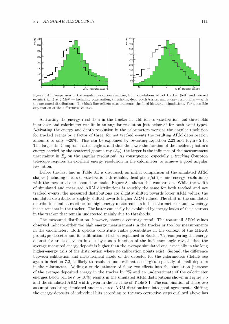
8.1. ANGULAR RESOLUTION 111
]°ARM - Compton cone [-6 -4 -2 0 2 4 6
coun
ts
50
100
150
200
250
300
350
400
]°ARM - Compton cone [-10 -5 0 5 10
coun
ts
50
100
150
200
250
300
350
400
450
Figure 8.4: Comparison of the angular resolution resulting from simulations of not tracked (left) and trackedevents (right) at 2 MeV — including voxelization, thresholds, dead pixels/strips, and energy resolutions — withthe measured distributions. The black line reflects measurements, the filled histogram simulations. For a possibleexplanation of the differences see text.
Activating the energy resolution in the tracker in addition to voxelization and thresholdsin tracker and calorimeter results in an angular resolution just below 3◦ for both event types.Activating the energy and depth resolution in the calorimeters worsens the angular resolutionfor tracked events by a factor of three; for not tracked events the resulting ARM deteriorationamounts to only ∼20%. This can be explained by revisiting Equation 2.23 and Figure 2.15:The larger the Compton scatter angle ϕ and thus the lower the fraction of the incident photon’senergy carried by the scattered gamma ray (Eg), the larger is the influence of the measurementuncertainty in Eg on the angular resolution! As consequence, especially a tracking Comptontelescope requires an excellent energy resolution in the calorimeter to achieve a good angularresolution.
Before the last line in Table 8.1 is discussed, an initial comparison of the simulated ARMshapes (including effects of voxelization, thresholds, dead pixels/strips, and energy resolutions)with the measured ones should be made. Figure 8.4 shows this comparison. While the widthof simulated and measured ARM distributions is roughly the same for both tracked and nottracked events, the measured distributions are slightly shifted towards lower ARM values, thesimulated distributions slightly shifted towards higher ARM values. The shift in the simulateddistributions indicates either too high energy measurements in the calorimeter or too low energymeasurements in the tracker. The latter can easily be explained by energy losses of the electronsin the tracker that remain undetected mainly due to thresholds.
The measured distribution, however, shows a contrary trend: The too-small ARM valuesobserved indicate either too high energy measurements in the tracker or too low measurementsin the calorimeter. Both options constitute viable possibilities in the context of the MEGAprototype detector and its calibration: First, as explained in Section 7.2, comparing the energydeposit for tracked events in one layer as a function of the incidence angle reveals that theaverage measured energy deposit is higher than the average simulated one, especially in the longhigher-energy tails of the distribution where no calibration points exist. Second, the differencebetween calibration and measurement mode of the detector for the calorimeters (details seeagain in Section 7.2) is likely to result in underestimated energies especially of small depositsin the calorimeter. Adding a crude estimate of these two effects into the simulation (increaseof the average deposited energy in the tracker by 7% and an underestimate of the calorimeterenergies below 511 keV by 10%) results in the simulated ARM distributions shown in Figure 8.5and the simulated ARM width given in the last line of Table 8.1. The combination of these twoassumptions bring simulated and measured ARM distributions into good agreement. Shiftingthe energy deposits of individual hits according to the two corrective steps outlined above has

112 CHAPTER 8. IMAGING PROPERTIES OF THE MEGA PROTOTYPE
]°ARM - Compton cone [-6 -4 -2 0 2 4 6
coun
ts
50
100
150
200
250
300
]°ARM - Compton cone [-10 -5 0 5 10
coun
ts
50
100
150
200
250
300
350
400
Figure 8.5: Comparison of the angular resolution of not tracked (left) and tracked events (right) with the measureddistributions at 2 MeV after accounting for an average overestimate of the energy in the tracker and a potentialunderestimate of the deposited energy in the calorimeter. The two corrections combined would explain thediscrepancy in the ARM peak positions between simulation and measurement evident in Figure 8.4. Again, theblack line reflects measurements, the filled histogram simulations.
no significant influence on the total simulated energy spectrum because the two effects almostcancel each other.
Much more detailed calibration measurements with the prototype would be required to quan-titatively assess these two effects from measurements and to correct the calibration for botheffects. Since the combination of both calibration deficiencies only shifts the ARM from theright to the left side of the axis, and since the shift is still small compared to the width of theARM distribution, no significant net effect on the width of reconstructed sources is expected.Thus the following discussion is using the original calibration obtained from Andritschke (2006).
8.1.1.2 Length of the Compton arc
For a tracking Compton telescope, the second characterizing feature is the length of the Comp-ton arc, either represented by the scatter plane deviation (SPD) or the electron ARM. In theCompton energy regime of the prototype, it is completely dominated by Moliere scattering.
Determining the electron ARM or SPD only for “photo peak” events of the Duke measure-ments is a drastic event cut: For the electron to be fully absorbed in the MEGA tracker, it musthave a low energy (< 2 MeV) — if the track is too long, the electron might escape from thetracker. In addition, the probability that at least one hit is missing from the track is increasingwith the track length. Selecting only events with electron tracks < 2 MeV, however, will resultin an electron ARM or SPD much broader than what would be observed for the average tracked
5
9
85
89
-5
-9
#5
#9
$5
5 - $ 6 7 85
=� �#��!�7�8
.*,�3>3��7$��8
".���������� ".�����������
5
85
-5
#5
$5
95
65
5 - $ 6 7 85
=� �#��!�7�8
������#��6��9>3��
7$��8
(�� �����<3���������
(�� �����<3����������
Figure 8.6: SPD: Comparison between simulation andreality.
Figure 8.7: Electron ARM: Comparison between sim-ulation and reality

8.1. ANGULAR RESOLUTION 113
]°[0 20 40 60 80 100 120 140 160 180
coun
ts
0
100
200
300
400
500
Figure 8.8: Comparison of thescatter plane deviation of the 2MeV measurement (thick line)with the simulation. Both arein agreement within measurementand simulation uncertainties.
]°SPD [0 20 40 60 80 100 120 140 160 180
]°C
ompt
on s
catte
r an
gle
[
0
10
20
30
40
50
60
70
80
90
Figure 8.9: Distribution of thescatter plane deviation versus theCompton scatter angle for the2 MeV run. The colors indicatea linear scale and each horizontalline has been normalized in thesum to one, to better show theshape of the scatter plane devia-tion.
Compton event at high energies: Small electron energies correspond to large electron scatterangles. For on-axis incidence, the scattered lower-energy electrons therefore must pass throughmore Silicon in one layer, increasing the effects of Moliere scattering.
Figure 8.6 shows the HWHM of the scatter plane deviation of tracked events for the Dukemeasurements at 2, 5 and 8 MeV, and Figure 8.7 shows the FWHM of the electron ARM, eachcompared to simulations. For both measures of the Compton arc length, simulation and mea-surement are in good agreement. The largest deviation appears at 8 MeV where measurementstatistics are lowest; within errors all measured electron ARM and SPD widths are in goodagreement with simulations.
Figure 8.8 illustrates the good agreement between simulation and measurements (thick line)of shape and width of the scatter plane deviation for the Duke 2 MeV on axis measurement.
Figure 8.9 shows the scatter plane deviation for “photo peak” events observed in the 2 MeVon-axis run as function of the Compton scatter angle. Two effects lead to an overall distributionwhich narrows with larger scatter angle: First, a large Compton scatter angle corresponds to alarger energy transfer to the electron, making Moliere scattering less influential. Second, largeCompton scatter angles lead to smaller electron scatter angles, which for on-axis photons meansthat the electron has to pass less material per layer and thus gets scattered less. The same

114 CHAPTER 8. IMAGING PROPERTIES OF THE MEGA PROTOTYPE
5
9
85
89
-5
5 85 -5 #5 $5 95 65
=� �#��!�7�8
?�:���#���# #����#�
7$��8
(�<(=
3(���������������� ����
3(��������������79B����������� ���
Figure 8.10: Comparison of the achieved angular resolution of the MEGA prototype and EGRET: At 49 MeV,MEGA’s angular resolution is almost a factor of two better than EGRET’s.
applies at higher energies, of course; however, not enough photo peak events have been collectedduring the Duke runs to compile a similar 2D scatter plot.
8.1.2 The pair regime
Pair events — previously discussed in Section 2.3 — have some advantages over Compton events.They can be directly reconstructed without the necessity to measure the energy to a very highaccuracy, and their response is in first order symmetric around the incident photon’s direction.Consequently, the angular resolution can be determined simply from the deviation of the calcu-lated from the real origin. The angular resolution of the MEGA prototype in the pair regime,given as the half-angle of a cone containing 68% of all reconstructed events for a given Dukerun, is shown in Figure 8.10.
The angular resolution of the MEGA prototype for pair events is dominated by the unknownrecoil of the nucleus and Moliere scattering in the Silicon layer of the pair creation. The influenceof both effects reduces with increasing photon energy (see also Figure 2.23). Thus the angularresolution improves with higher energies.
Figure 8.10 shows the angular resolution without and with cuts on the pair opening angle. Nocuts on the measured photon energy were applied. The 68% containment has been determinedin each case from an angular resolution plot such as that shown in Figure 8.11.
]°Angular resolution [0 10 20 30 40 50 60 70 80 90
coun
ts
0
2000
4000
6000
8000
10000
12000
14000
16000
]°Opening angle [0 10 20 30 40 50 60 70 80 90
coun
ts
0
5000
10000
15000
20000
25000
30000
Figure 8.11: Distribution of the angular deviation be-tween the measured and real origin of the pair photon.
Figure 8.12: Opening angle distribution of all pairevents recorded in the 49 MeV on-axis measurement.

8.1. ANGULAR RESOLUTION 115
Between the opening angle and the probability that the pair has been reconstructed correctlyexists a correlation: Larger opening angles correspond to a more uneven distribution of thephoton’s energy to the pair’s electron and positron. The more the electron and positron anglesdiffer, however, the more significant the energy correction to the reconstructed photon directionbecomes (compare Equation 2.28). Since the majority of pair events is not even marginallycontained in the prototype, the simpler direction reconstruction based on Equation 2.29 resultsin a better angular resolution than those using the energies. As a consequence, the incidentphoton direction of pairs with large opening angles is not correctly reconstructed. Moreover,events in the tail of the distribution of reconstructed opening angles (see Figure 8.12) are partlyreconstructed incorrectly — for example when the true vertex start point is missing, and ahit lower in one of the two particle tracks is used as vertex start point. This can be verifiedboth using simulations and by backprojecting such events onto the sky. Both effects results ina fairly random distribution on the sky for large opening angles (e.g. > 50◦ for the 49 MeVmeasurement), rather than one clustered around the incident photon direction. Consequently,using only the 85% of events with the smallest opening angles results in a significant improvement(on average 20%) of the angular resolution for pair events. This opening angle cut rejects allangles larger than 23◦ at 49 MeV and all larger than 45◦ at 12 MeV. It will be used as one ofthe background rejection cuts for the MEGA satellite in Chapter 10.
At 49 MeV the MEGA prototype’s angular resolution is roughly a factor two better thanEGRET’s (top graph in Figure 8.10). MEGA will also surpass the expected angular resolutionperformance of GLAST and AGILE since they — same as EGRET — contain converter foilswhich increase the angular dispersion due to Moliere scattering.
5
-
$
6
7
85
8-
5 85 -5 #5 $5 95 65
=� �#��!�7�8
?�:���#���# #����#�
7$��8
3(��������������79B����������� ���
3(������������79B����������� ���
Figure 8.13: Comparison of the simulated angular res-olution in the pair regime with that achieved analyzingMEGA prototype measurements.
Figure 8.13 compares the simulated angular resolution with the measured one. Generally,the simulated angular resolution is slightly better than the measured one. The difference ismore pronounced at lower energies. The simulation does not take into account the recoil of thenucleus, and so a slightly better performance of the simulation is expected. A larger fractionof the total photon momentum is transferred to the nucleus at lower energies. Therefore, theresulting discrepancy between simulation and measurement is largest in this regime. However,the missing energy transfer to the recoil nucleus cannot fully explain the observed deviation. Theremainder of the discrepancy is likely caused by problematic events in the Duke measurementdata — arising either from contamination of the beam by charged particles and/or higher-energyphotons, or from interactions of the photon beam in a cover above the tracker that was left inplace during the high-energy beam runs and whose honeycomb structure could not satisfactorilybe represented in the model geometry.
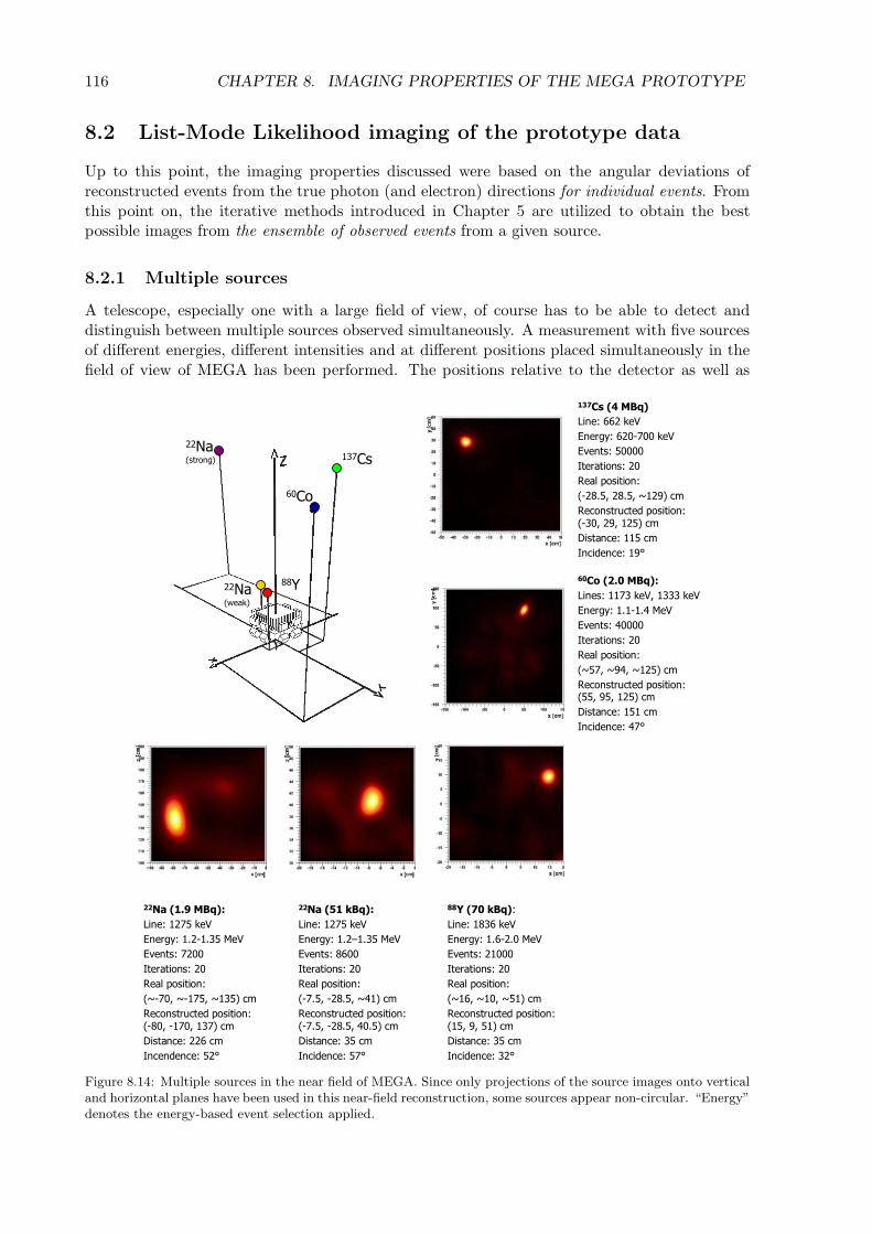
116 CHAPTER 8. IMAGING PROPERTIES OF THE MEGA PROTOTYPE
8.2 List-Mode Likelihood imaging of the prototype data
Up to this point, the imaging properties discussed were based on the angular deviations ofreconstructed events from the true photon (and electron) directions for individual events. Fromthis point on, the iterative methods introduced in Chapter 5 are utilized to obtain the bestpossible images from the ensemble of observed events from a given source.
8.2.1 Multiple sources
A telescope, especially one with a large field of view, of course has to be able to detect anddistinguish between multiple sources observed simultaneously. A measurement with five sourcesof different energies, different intensities and at different positions placed simultaneously in thefield of view of MEGA has been performed. The positions relative to the detector as well as
����������� ������������ �������� ��������������� �������������������������������� ��������!"#��"$���"�#%�&'��&�����(&��)� ���������!##��$#���#%�&'*�����&���#�&'��&�)��&����+
����������� ������,,���� ��������,�������� ��������#����������������������� ��������!��-�#���-�#��"�$%�&'��&�����(&��)� ���������!������$���#%�&'*�����&���#�&'��&�)��&���$+
����������� ��������-�,��� ���������,������� ������������������������������� ��������!",��"���"#%�&'��&�����(&��)� ���������!#��$��#%�&'*�����&����#�&'��&�)��&�����+
����������� ��������#��� �������������#��� ������������������������������ ��������!"����"�#��"�#%�&'���&�����(&��)� ���������!�-��������%�&'*�����&�����,�&'��&��)��&���#�+
������������ ��������#��� ����������.��#��� ��������-,��������������������� ��������!��#����-�#��"�%�&'��&�����(&��)� ���������!��#����-�#�����#%�&'*�����&����#�&'��&�)��&���#+
�/�
,�/�
��0�!������%
��0�!1���%
--2
Figure 8.14: Multiple sources in the near field of MEGA. Since only projections of the source images onto verticaland horizontal planes have been used in this near-field reconstruction, some sources appear non-circular. “Energy”denotes the energy-based event selection applied.

8.2. LIST-MODE LIKELIHOOD IMAGING OF THE PROTOTYPE DATA 117
Figure 8.15: Thepropeller on top ofthe MEGA Styrofoamhousing.
� � �� ���������� � � �� ����������
�
��
���
���
��
��
�
���
Figure 8.16: “Radioactive ring”: In the image at iteration 0 (left), which is only a simple back projection of theevents, the ring structure is hidden by cone circles and arcs. The ring structure is clearly visible after 50 iterationswith the list-mode algorithm (right).
the reconstructed near-field images are shown in Figure 8.14. All five sources have been imagedto their correct positions. This measurement proves MEGA’s capability to disentangle multiplesources and also serves to illustrate its large field of view at low energies.
8.2.2 Extended sources
The sky in the MeV regime contains a host of extended source regions, from supernova remnantsand OB-associations to our Galaxy as a whole, in addition to a multitude of point sources.Therefore the ability to image extended sources is a key requirement for any telescope formedium-energy gamma-ray astronomy. The capability of the MEGA prototype in conjunc-tion with the List-Mode Maximum-Likelihood Expectation-Maximization algorithm to imageextended sources can be illustrated using laboratory measurements. Two 88Y sources (34 kBqand 36 kBq) have been mounted on a rotating propeller located 27 cm above the center of theMEGA prototype’s tracker on the Styrofoam cover of the detector. The propeller swept out acircle with radius 7 cm, which corresponds to a diameter of ∼29◦. The setup is illustrated inFigure 8.15.
The reconstructed image (left 0th iteration, right 50th iteration of the LM-ML-EM algorithm)can be found in Figure 8.16. It contains ∼138,000 Compton events in the energy range from 0.8

118 CHAPTER 8. IMAGING PROPERTIES OF THE MEGA PROTOTYPE
710 keV
Figure 8.17: Right column: Images oftracked events from 2 to 8 MeV: At2 MeV the image is dominated by theenergy resolution in the calorimeters,which dominates all other resolutions byroughly a factor 3. At higher energies,this factor becomes less important, andthe overall angular resolution improvessignificantly. The deviation of the shapeof the source from perfect symmetry isdue to the low statistics at 5 MeV and8 MeV (187 events at 8 MeV).
2 MeV
5 MeV
Figure 8.18: Left column: Images of nottracked events at 710 keV and 2 MeV.While at 710 keV the angular resolu-tion is dominated by the energy reso-lution in the calorimeters, at 2 MeV itis dominated by the position resolutionin the calorimeters, which contributes∼60% to the angular resolution at thisenergy.
8 MeV

8.2. LIST-MODE LIKELIHOOD IMAGING OF THE PROTOTYPE DATA 119
to 1.0 MeV. The minor irregularities in the imaged circle result from the assumption that alldetectors have the same efficiency.
This measurement constitutes a perfect demonstration of the performance of the imagingalgorithm: The left image shows the zeroth iteration of the list-mode maximum-likelihoodexpectation-maximization algorithm. The overlapping raw Compton cones let the source ap-pear disk-like. With higher iterations, the ring structure becomes visible. The algorithm washalted when the width of the ring roughly corresponded to the angular resolution achieved bythe MEGA prototype.
8.2.3 On axis imaging as a function of energy
Figures 8.17 and 8.18 show the reconstructed Duke images in the Compton regime from 710 keVup to 8 MeV for on-axis measurements, split into tracked and not tracked events. Only two-siteevents were used to generate the images, which nicely illustrate the improvement in angularresolution towards higher energies promised by the decreasing ARM width illustrated in Figure8.3.
Figure 8.19 shows reconstructed images for on-axis incidence in the pair regime (12 to49 MeV). With increasing beam energy, the reconstructed source image becomes sharper, be-cause the influence of both the unknown recoil of the nucleus and Moliere scattering weaken.
8.2.4 Field of view
One large advantage of both Compton and pair telescopes is their large field of view. Figure 8.20contains reconstructed images at incidence angles from 0◦ to 60◦ at 5 MeV and from 0◦ to 80◦
at 49 MeV, demonstrating the large field of view of the MEGA prototype in the Compton andpair regimes.
12 MeV 17 MeV 25 MeV
37 MeV 49 MeV
Figure 8.19: Images of reconstructedon-axis beam sources in the pairregime. With increasing energy thesource images become sharper sinceat higher energies Moliere scatteringis less pronounced and the unknownrecoil of the nucleus does no longerplay a significant role.

120 CHAPTER 8. IMAGING PROPERTIES OF THE MEGA PROTOTYPE
5 MeV tracked Compton events 49 MeV pair events
0◦
30◦
60◦
80◦
Figure 8.20: Field of view of the MEGA prototype for tracked Compton events at 5 MeV and pair events at49 MeV.
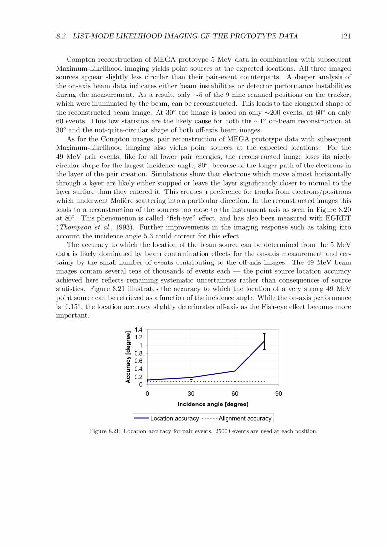
8.2. LIST-MODE LIKELIHOOD IMAGING OF THE PROTOTYPE DATA 121
Compton reconstruction of MEGA prototype 5 MeV data in combination with subsequentMaximum-Likelihood imaging yields point sources at the expected locations. All three imagedsources appear slightly less circular than their pair-event counterparts. A deeper analysis ofthe on-axis beam data indicates either beam instabilities or detector performance instabilitiesduring the measurement. As a result, only ∼5 of the 9 nine scanned positions on the tracker,which were illuminated by the beam, can be reconstructed. This leads to the elongated shape ofthe reconstructed beam image. At 30◦ the image is based on only ∼200 events, at 60◦ on only60 events. Thus low statistics are the likely cause for both the ∼1◦ off-beam reconstruction at30◦ and the not-quite-circular shape of both off-axis beam images.
As for the Compton images, pair reconstruction of MEGA prototype data with subsequentMaximum-Likelihood imaging also yields point sources at the expected locations. For the49 MeV pair events, like for all lower pair energies, the reconstructed image loses its nicelycircular shape for the largest incidence angle, 80◦, because of the longer path of the electrons inthe layer of the pair creation. Simulations show that electrons which move almost horizontallythrough a layer are likely either stopped or leave the layer significantly closer to normal to thelayer surface than they entered it. This creates a preference for tracks from electrons/positronswhich underwent Moliere scattering into a particular direction. In the reconstructed images thisleads to a reconstruction of the sources too close to the instrument axis as seen in Figure 8.20at 80◦. This phenomenon is called “fish-eye” effect, and has also been measured with EGRET(Thompson et al., 1993). Further improvements in the imaging response such as taking intoaccount the incidence angle 5.3 could correct for this effect.
The accuracy to which the location of the beam source can be determined from the 5 MeVdata is likely dominated by beam contamination effects for the on-axis measurement and cer-tainly by the small number of events contributing to the off-axis images. The 49 MeV beamimages contain several tens of thousands of events each — the point source location accuracyachieved here reflects remaining systematic uncertainties rather than consequences of sourcestatistics. Figure 8.21 illustrates the accuracy to which the location of a very strong 49 MeVpoint source can be retrieved as a function of the incidence angle. While the on-axis performanceis 0.15◦, the location accuracy slightly deteriorates off-axis as the Fish-eye effect becomes moreimportant.
5
5�-
5�$
5�6
5�7
8
8�-
8�$
5 #5 65 ;5
"#��$#���#���7$��8
���&���!�7$��8
+� ���� �� � ��������� �� �
Figure 8.21: Location accuracy for pair events. 25000 events are used at each position.

122 CHAPTER 8. IMAGING PROPERTIES OF THE MEGA PROTOTYPE

Chapter 9
The MEGA prototype as Comptonpolarimeter
Most processes in high energy astrophysics, such as synchrotron radiation, bremsstrahlung, orCompton scattering, generate polarized gamma rays. All past and present gamma-ray telescopes,however, have at best limited capabilities to detect this polarization. A MEGA-like telescope,ideally suited to detect polarized gamma rays in the Compton regime, would provide a valuabletool for constraining emission geometries and source magnetic field configurations and thusenable a better understanding of the source emission mechanisms.
As described in section 6.2, all measurements during the Duke campaign were performed withmonoenergetic 100% polarized pencil beams of gamma rays with a fixed, horizontal polarizationvector. This beam is well suited to determine the polarization response of the MEGA prototype.
9.1 Data correction
To retrieve the expected polarization signal (see Chapter 2.2.3) from the raw azimuthal scatterangle distribution, three corrections have to be applied: for individual detector module efficiency,detector geometry, and background.
In the ideal case one measurement with a 100% linearly polarized photon beam and one witha non-polarized beam under otherwise identical would be required to allow optimum correctionfor efficiency and geometry. Due to the production process of the gamma rays (100% linearlypolarized IR or UV photons are Compton backscattered), it was not possible to turn off thepolarization of the beam at Duke. Other simple correction techniques, like rotating the detectoror the polarization vector to effectively remove the polarization could not be applied either.
Measurements with radioactive laboratory sources, which are of course unpolarized, at en-ergies similar to the Duke beams are one possibility for the corrections. However, due to (1)detector efficiencies strongly varying between the measurements in Garching and in Duke, (2)problems correcting far-field (Duke) with near-field (Garching) measurements and (3) not 100%identical energies (710 keV beam vs. 662 keV line of 137Cs and 2.0 MeV beam vs. 1.8 MeV line of88Y), the laboratory measurements alone are not sufficient to perform all necessary corrections.
Consequently a more complex approach had to be chosen to correct the data. It relies partlyon event selections, partly on laboratory calibrations, and partly on simulations: The mostdisturbing problem is caused by time-varying trigger and read-out thresholds in the calorimeters(see Chapter 6) which effectively result in time-variable efficiencies of the calorimeters. Toovercome this problem, only those events were selected which have at least a deposit of 300keV in one single crystal. Since low energies of the scattered gamma ray correspond to largescatter angles, this selection leads to a restriction to smaller scatter angles and thus the detected
123
124 CHAPTER 9. THE MEGA PROTOTYPE AS COMPTON POLARIMETER
polarization signature decreases. After this selection, all remaining differences are expected tobe time invariant, like defective pixels or the coupling between crystals and PIN-diodes. So theremaining efficiency correction can be applied using previous lab measurements.
The largest influence on the azimuthal shape is due to the geometry. At low energies the holesbetween individual calorimeter modules are visible in the azimuthal scatter angle distribution.At higher energies the four edges of the bottom calorimeter are visible. Since no suitableunpolarized measurement was available, the geometry correction was taken from simulations.
The background does not need a correction since it can be easily suppressed by data cuts:Firstly, selecting only events from the known path of the tightly collimated beam eliminatespractically all of the room background (especially the 1.461 MeV line of 40K). Secondly, incom-pletely absorbed events and chance coincidences are eliminated (1) by the event reconstruction,(2) by selecting only events originating from the known source direction and (3) by using onlyevents with the correct energy.
Thus the final correction applied to the data was:
Pcorr(χ) =Pmeas(χ)
Pgeo(χ)Peff (χ,ϕ)(9.1)
where Pmeas is the raw, measured and Pcorr is the corrected azimuthal scatter angle distribution(details see Section 2.2.3) as a function of the azimuthal Compton scatter angle χ. Pgeo(χ) isthe geometry correction discussed above, and Peff (χ,ϕ) is the described efficiency correction.
9.2 Polarization response of the prototype
As explained in Section 2.2.3 and illustrated in Figure 2.8, the polarization response of a Comp-ton telescope has two main properties which of course should be visible in the MEGA mea-surements: The modulation as a function of energy has to increase towards lower energies. Asa function of Compton scatter angles it has to reach its maximum at medium scatter angles(below 90◦, depending on energy).
The measured energy dependence of the modulation for the Duke measurements at 0.71, 2and 5 MeV is illustrated in Figure 9.1. If no Compton scatter angle selections are applied, themodulation decreases from 0.17 at 0.71 MeV to 0.12 at 2 MeV down to 0.06 at 5 MeV. At 8 MeVno significant modulation is seen. All these values are in good agreement with simulations.
The polarization vector of the Duke beam was horizontally aligned in the room and thereforethe maxima of the measured modulation are expected in the vertical direction. Thus the minima,which correspond to the polarization angle, have to be found at 90◦ in Figure 9.1. The measuredvalues, 82◦ ± 24◦ at 0.7 MeV, 86◦ ± 11◦ at 2 MeV and 74◦ ± 18◦ at 5 MeV, are all compatiblewith a 90◦ polarization vector within measurement errors. At 2 MeV, measurement errors aresmallest and the measured polarization angle agrees well with the beam’s polarization vector.The large error — and large deviation of the measured polarization angle — at 5 MeV can beexplained by the weak polarization signal and the poor statistics. At 0.71 MeV the deviation ismainly due to varying efficiencies of individual detector modules.
Since the source signal dominates the background and since only one source is present, forthese measurements it is also possible to do a polarization calculation without the necessity ofimaging the event into the source location and without restricting the energy. For example,∼50% of the events at 710 keV cannot be imaged into the point source, although their firstinteraction is within the beam path. The reasons are mainly incomplete absorption in the trackeror calorimeter, but also problems measuring the correct energy for small hits in the calorimeters.Events with low-energy calorimeter hits carry most of the polarization information, but nocorrect calorimeter calibration below 511 keV exists. Moreover, due to the difference betweenthe calibration and measurement mode (details see 7.2 and Andritschke, 2006) it is likely that

9.2. POLARIZATION RESPONSE OF THE PROTOTYPE 125
]° [χAzimuthal scatter angle 0 50 100 150
Res
idua
ls
-0.3
-0.2
-0.1
0
0.1
0.2
0.3
0.4
0.5 0.7 MeV
]° [χAzimuthal scatter angle 0 50 100 150
Res
idua
ls
-0.2
-0.15
-0.1
-0.05
-0
0.05
0.1
0.15
0.2 2.0 MeV
]° [χAzimuthal scatter angle 0 50 100 150
Res
idua
ls
-0.2
-0.1
0
0.1
0.2
0.3 5.0 MeV
Figure 9.1: Polarization response as a function of en-ergy: The black line indicates the best fit with a cosine.The origin of the scatter angle x-axis corresponds to thevertical direction as MEGA is mounted at HIGS. Withinmeasurement errors and statistics, all values are in agree-ment with the simulations (see table below).
Modulation μ Polarization angle [◦]Energy [MeV]measured simulated measured simulated
0.71 0.17 ± 0.04 0.19 82 ± 24 902.0 0.13 ± 0.03 0.14 86 ± 11 905.0 0.06 ± 0.03 0.03 74 ± 18 90
the total measured energy is lower than the real one. The latter is easily verified by lookingat the spectrum for the 710 keV measurement when only energies of the scattered gamma-raybelow e.g. 450 keV (scatter angles larger 54◦) are allowed. There no photo-peak is visible.
If no kinematics restrictions are applied, and only the azimuthal scatter angle is determinedgeometrically from the two interaction positions, the modulation can also be determined. Onlyan upper energy cut has to be applied to suppress background from the beam itself as well asfrom the concrete walls (40K).
This method results in a modulation of 0.30 ± 0.08 at 710 keV, which is almost a factor2 higher than that obtained using the initial event selections, but suffers from a much higheruncertainty. Since at higher energies the suppression of larger scatter angles does not play adominant role, at 2 MeV and above the two methods yield the same results within measurementerrors.
The modulation as a function of the Compton scatter angle is shown in Figure 9.2 forthe 2 MeV measurement. As expected, the modulation reaches its maximum around 66◦; themeasurement is in good agreement with the simulations.
The prototype clearly demonstrates that MEGA is a perfect polarimeter in the Comptonregime. The well-chosen geometry of MEGA allows it to detect Compton events with largescatter angles; these carry most of the polarization information. An envisioned MEGA satellitetelescope will probably be able to measure photons down to ∼300 keV, where the polarization

126 CHAPTER 9. THE MEGA PROTOTYPE AS COMPTON POLARIMETER
]° [ϕCompton scatter angle 0 20 40 60 80 100
μM
odul
atio
n
0
0.05
0.1
0.15
0.2
0.25
0.3
0.35
]° [ϕCompton scatter angle 0 20 40 60 80 100
μM
odul
atio
n
0
0.05
0.1
0.15
0.2
0.25
0.3
0.35
Modulation μAngle ϕ [◦]measured simulated
10 0.04 ± 0.03 0.0535 0.16 ± 0.03 0.1765 0.28 ± 0.03 0.2695 0.20 ± 0.08 0.23
Figure 9.2: Dependence of the modulation on the Compton scatter angle for 2 MeV photons. The trianglesrepresent the values from Geant4 simulations, which are in good agreement with the measurements. The maximumis reached as expected around 66◦. At 95◦, poor statistics lead to a larger measurement error.
information of the original photons is best preserved through the Compton scatter process. WhileMEGA will not be able to distinguish these low energy photons from background in normaloperation mode, for special sources such as gamma-ray bursts or solar flares the polarizationproperties can be easily determined: They are short and strong events for which the backgrounddoes not play a dominating role. MEGA will add a new dimension to gamma-ray astronomy —polarization!

Part IV
Steps towards a MEGA spacemission
127

128
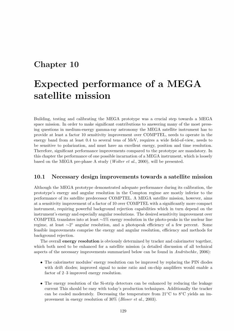
Chapter 10
Expected performance of a MEGAsatellite mission
Building, testing and calibrating the MEGA prototype was a crucial step towards a MEGAspace mission. In order to make significant contributions to answering many of the most press-ing questions in medium-energy gamma-ray astronomy the MEGA satellite instrument has toprovide at least a factor 10 sensitivity improvement over COMPTEL, needs to operate in theenergy band from at least 0.4 to several tens of MeV, requires a wide field-of-view, needs tobe sensitive to polarization, and must have an excellent energy, position and time resolution.Therefore, significant performance improvements compared to the prototype are mandatory. Inthis chapter the performance of one possible incarnation of a MEGA instrument, which is looselybased on the MEGA pre-phase A study (Wolter et al., 2000), will be presented.
10.1 Necessary design improvements towards a satellite mission
Although the MEGA prototype demonstrated adequate performance during its calibration, theprototype’s energy and angular resolution in the Compton regime are mostly inferior to theperformance of its satellite predecessor COMPTEL. A MEGA satellite mission, however, aimsat a sensitivity improvement of a factor of 10 over COMPTEL with a significantly more compactinstrument, requiring powerful background rejection capabilities which in turn depend on theinstrument’s energy and especially angular resolutions. The desired sensitivity improvement overCOMPTEL translates into at least ∼5% energy resolution in the photo-peaks in the nuclear lineregime, at least ∼2◦ angular resolution, and a photopeak efficiency of a few percent. Somefeasible improvements comprise the energy and angular resolution, efficiency and methods forbackground rejection.
The overall energy resolution is obviously determined by tracker and calorimeter together,which both need to be enhanced for a satellite mission (a detailed discussion of all technicalaspects of the necessary improvements summarized below can be found in Andritschke, 2006):
• The calorimeter modules’ energy resolution can be improved by replacing the PIN diodeswith drift diodes; improved signal to noise ratio and on-chip amplifiers would enable afactor of 2–3 improved energy resolution.
• The energy resolution of the Si-strip detectors can be enhanced by reducing the leakagecurrent This should be easy with today’s production techniques. Additionally the trackercan be cooled moderately. Decreasing the temperature from 21◦C to 8◦C yields an im-provement in energy resolution of 30% (Bloser et al., 2003).
129

130 CHAPTER 10. EXPECTED PERFORMANCE OF A MEGA SATELLITE MISSION
• In a future read-out system temperature instabilities, varying trigger thresholds, system-atic errors due to delicate timing, etc. will be significantly reduced to improve the energyresolution.
The angular resolution is influenced by detector position resolution and Doppler broaden-ing as well as energy resolution. While a Silicon tracker is already the best choice of currentlyavailable semi-conductor materials as far as Doppler-broadening is concerned, the following im-provements are possible:
• For tracking Compton telescopes, which predominantly track Compton events with largeCompton scatter angles, the energy resolution of the second detector system is more im-portant than that of the first one (compare Figures 2.14 and 2.15 for large scatter angles).Therefore, more efforts should be devoted to improving the calorimeter modules’ energyresolution.
• While the position resolution of the tracker is more than sufficient, the position resolutionof the calorimeter, especially the depth resolution, is not. For a much larger satellitedetector, the average distance between the tracker and calorimeter interactions increasesand the problem partly resolves itself. In addition, switching from PIN to drift diodes inthe calorimeter would not only improve the energy resolution but also the depth resolution.Moreover, a careful roughening of the surface of the crystals would lead to an increasedlight output gradient along the CsI bars. Since this sacrifices part of the light yield andthus energy resolution, a detailed trade-off analysis is required.
The efficiency of a detector is determined by the fraction of incoming photons whose incidentdirection and energy is correctly reconstructed to within the instrument’s angular and energyresolution.
• The first measure to increase the number of photons detected in a D1-D2 hit sequence isto build a deeper tracker in which significantly more photons have their first interaction.Currently only 0.7 percent of all on-axis 2 MeV photons, which generate a D1-D2 triggerhave their first interaction in the tracker.
• As a second step, the calorimeter has to be constructed in a more compact fashion: Whilethe calorimeter of the prototype covers only ∼30% of the lower hemisphere, the finalversion should cover ∼100%.
• Additionally, reducing the amount of passive material inside the detector head results inan increased number of events completely absorbed in active detector material. Thus itis very important to reduce as much as possible all materials on the path of the photonsto their interaction in the tracker and on their way to the calorimeter (minimize mechan-ical structure of D1 and its surrounding electronics, make a thin entry window into thecalorimeter, etc.).
• One of the limiting factors for the prototype’s efficiency is the high dead time of thereadout, which limits the detectable event rate to roughly 130 cts/s. A simple advancewould be to read out all chips in parallel instead of in series, and/or to read out onlychannels with signals above the noise threshold.
• Due to the high thresholds in the detectors a lot of interactions with small energy depositsare lost. This is particularly problematic for the start point of a Compton electron track,which has a probability of ∼25% percent to go undetected in the prototype — only thepassage of the electron through the next layers is detected, leading to missing energy,decreased position resolution, and a higher risk of wrongly reconstructing the event. Mostof the strategies to improve the energy resolution will also enable lower thresholds.
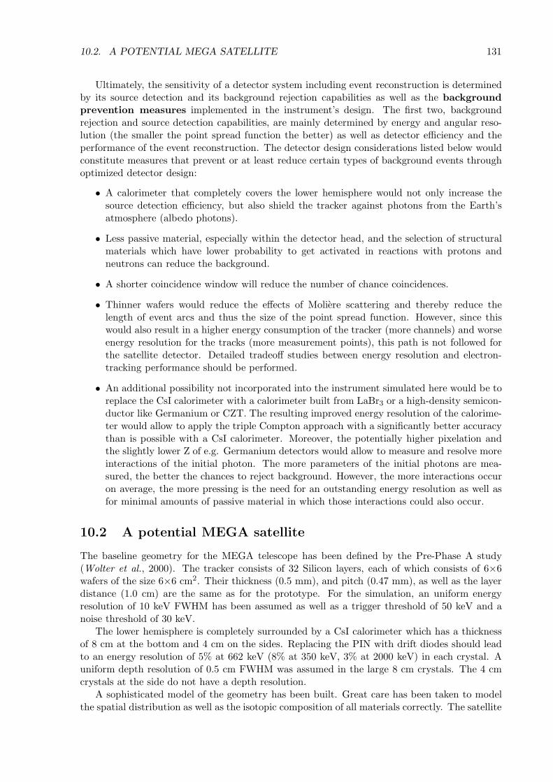
10.2. A POTENTIAL MEGA SATELLITE 131
Ultimately, the sensitivity of a detector system including event reconstruction is determinedby its source detection and its background rejection capabilities as well as the backgroundprevention measures implemented in the instrument’s design. The first two, backgroundrejection and source detection capabilities, are mainly determined by energy and angular reso-lution (the smaller the point spread function the better) as well as detector efficiency and theperformance of the event reconstruction. The detector design considerations listed below wouldconstitute measures that prevent or at least reduce certain types of background events throughoptimized detector design:
• A calorimeter that completely covers the lower hemisphere would not only increase thesource detection efficiency, but also shield the tracker against photons from the Earth’satmosphere (albedo photons).
• Less passive material, especially within the detector head, and the selection of structuralmaterials which have lower probability to get activated in reactions with protons andneutrons can reduce the background.
• A shorter coincidence window will reduce the number of chance coincidences.
• Thinner wafers would reduce the effects of Moliere scattering and thereby reduce thelength of event arcs and thus the size of the point spread function. However, since thiswould also result in a higher energy consumption of the tracker (more channels) and worseenergy resolution for the tracks (more measurement points), this path is not followed forthe satellite detector. Detailed tradeoff studies between energy resolution and electron-tracking performance should be performed.
• An additional possibility not incorporated into the instrument simulated here would be toreplace the CsI calorimeter with a calorimeter built from LaBr3 or a high-density semicon-ductor like Germanium or CZT. The resulting improved energy resolution of the calorime-ter would allow to apply the triple Compton approach with a significantly better accuracythan is possible with a CsI calorimeter. Moreover, the potentially higher pixelation andthe slightly lower Z of e.g. Germanium detectors would allow to measure and resolve moreinteractions of the initial photon. The more parameters of the initial photons are mea-sured, the better the chances to reject background. However, the more interactions occuron average, the more pressing is the need for an outstanding energy resolution as well asfor minimal amounts of passive material in which those interactions could also occur.
10.2 A potential MEGA satellite
The baseline geometry for the MEGA telescope has been defined by the Pre-Phase A study(Wolter et al., 2000). The tracker consists of 32 Silicon layers, each of which consists of 6×6wafers of the size 6×6 cm2. Their thickness (0.5 mm), and pitch (0.47 mm), as well as the layerdistance (1.0 cm) are the same as for the prototype. For the simulation, an uniform energyresolution of 10 keV FWHM has been assumed as well as a trigger threshold of 50 keV and anoise threshold of 30 keV.
The lower hemisphere is completely surrounded by a CsI calorimeter which has a thicknessof 8 cm at the bottom and 4 cm on the sides. Replacing the PIN with drift diodes should leadto an energy resolution of 5% at 662 keV (8% at 350 keV, 3% at 2000 keV) in each crystal. Auniform depth resolution of 0.5 cm FWHM was assumed in the large 8 cm crystals. The 4 cmcrystals at the side do not have a depth resolution.
A sophisticated model of the geometry has been built. Great care has been taken to modelthe spatial distribution as well as the isotopic composition of all materials correctly. The satellite
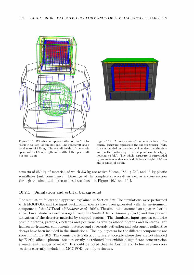
132 CHAPTER 10. EXPECTED PERFORMANCE OF A MEGA SATELLITE MISSION
Figure 10.1: Wire-frame representation of the MEGAsatellite as used for simulations. The spacecraft has atotal mass of 850 kg. The overall height of the wholespacecraft is 1.8 m; length and width of the spacecraftbus are 1.4 m.
Figure 10.2: Cutaway view of the detector head. Thecentral structure represents the Silicon tracker (red).It is surrounded on the sides by 4 cm deep calorimetersand on the bottom by 8 cm deep calorimeters (greyhousing visible). The whole structure is surroundedby an anti-coincidence shield. It has a height of 55 cmand a width of 65 cm.
consists of 850 kg of material, of which 5.3 kg are active Silicon, 183 kg CsI, and 16 kg plasticscintillator (anti coincidence). Drawings of the complete spacecraft as well as a cross sectionthrough the simulated detector head are shown in Figures 10.1 and 10.2.
10.2.1 Simulation and orbital background
The simulation follows the approach explained in Section 3.2: The simulations were performedwith MGGPOD, and the input background spectra have been generated with the environmentcomponent of the ACTtools (Wunderer et al., 2006). The simulation assumed an equatorial orbitat 525 km altitude to avoid passage through the South Atlantic Anomaly (SAA) and thus preventactivation of the detector material by trapped protons. The simulated input spectra comprisecosmic photons, protons, electrons and positrons as well as albedo photons and neutrons. Forhadron environment components, detector and spacecraft activation and subsequent radioactivedecays have been included in the simulations. The input spectra for the different components areshown in Figure 10.3. The cosmic particle distributions are isotropic where they are not shieldedby Earth; albedo photons are not evenly distributed but exhibit a significant concentrationaround zenith angles of ∼120◦. It should be noted that the Cesium and Iodine neutron crosssections currently included in MGGPOD are only estimates.

10.2. A POTENTIAL MEGA SATELLITE 133
Energy [keV]1 10 210 310 410 510 610 710 810
Energy [keV]1 10 210 310 410 510 610 710 810
/s/k
eV]
2/c
mγ
Flu
x [
-1610
-1410
-1210
-1010
-810
-610
-410
-210
1
210
410
510
Energy [keV]1 10 210 310 410 510 610 710 810
Energy [keV]1 10 210 310 410 510 610 710 810
/s/k
eV]
2/c
mγ
Flu
x [
-1610
-1410
-1210
-1010
-810
-610
-410
-210
1
210
410
510
Albedo Neutron
Albedo Neutron
Albedo Photon
Cosmic Electron
Cosmic Photon
Cosmic Positron
Cosmic Proton
Albedo Neutron
Albedo Photon
Cosmic Electron
Cosmic Photon
Cosmic Positron
Cosmic Proton
Albedo Neutron
Albedo Photon
Cosmic Electron
Cosmic Photon
Cosmic Positron
Cosmic Proton
Albedo Neutron
Albedo Photon
Cosmic Electron
Cosmic Photon
Cosmic Positron
Cosmic Proton
Albedo Neutron
Albedo Photon
Cosmic Electron
Cosmic Photon
Cosmic Positron
Cosmic Proton
Albedo Neutron
Albedo Photon
Cosmic Electron
Cosmic Photon
Cosmic Positron
Cosmic Proton
Albedo Neutron
Figure 10.3: Integrated inputspectra for the background simu-lations. Due to the geomagneticcutoff, charged particles need atleast an energy of 10 GeV toreach the spacecraft.
10.2.2 Event selections
For the event reconstruction of the simulated MEGA satellite data, the Bayesian approach hasbeen used. Detailed response matrices for electron tracking and Compton sequence reconstruc-tion as described in Chapter 4 have been calculated to enable this elaborate event reconstructionapproach and consequently provide the best background rejection available.
However, having used this elaborate event reconstruction approach does not imply that allreconstructed events should be used in the analysis. For the ultimate goal, determining thebest point-source sensitivity achievable with the MEGA instrument, several key backgroundrejection cuts have to be made. Evaluating the instrument’s point source sensitivity necessitatesa selection on a “resolution element window” around the (assumed known) source position. Fornot tracked events this window constitutes an ARM window, for tracked events an ARM andSPD window. For the case of gamma-ray line sources, an energy window is also necessary aspart of this basic set of selections. A second class of event cuts chooses only the “best” events,i.e. those defined by small Compton scatter angles, good Compton and track quality factors, aswell as a not too large dϑ value.
In addition, measures must be taken to reduce as much as possible the largest backgroundcomponent which are photons generated by cosmic-ray interactions in the Earth’s atmosphere.To achieve this, a so-called Earth horizon cut is introduced: For each event the probability iscalculated that it originates from the Earth’s atmosphere. The current algorithm determinesthe fraction of the event origin probability distribution (the Compton circle or arc) which iscompatible with an origin in the Earth’s atmosphere. If this value is too large, then the eventis rejected.
For pair events, two selection criteria are implemented: one on the opening angle (anglebetween the direction of electron and positron), the other on the energy deposit in the first layer— the higher the energy deposit, the longer was the electron/positron path in the first layer; theresulting more significant Moliere scattering finally results in a larger angular deviation fromthe true origin.
Most of the cuts are a function of energy, thus their optimum values have to be determined foreach nuclear line of interest or, for continuum sensitivity calculations, for each energy interval.Moreover, it is not obvious what the ideal values — i.e. those which optimize the sensitivity —are for e.g. a given astrophysical line and the background below this line. Thus a 13-dimensionalevent selection data space has to be searched for the optimum selections. This is accomplishedby calculating the sensitivity for each bin in this data space. Some selected results, for narrow
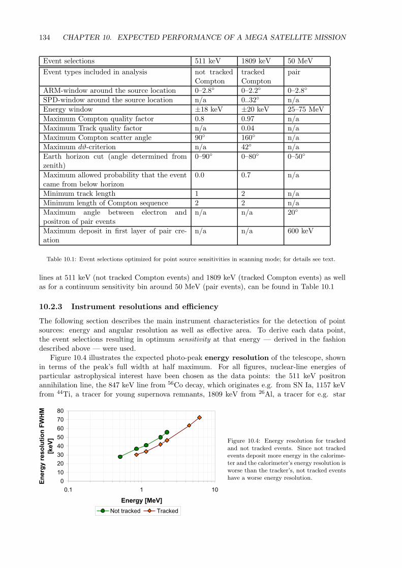
134 CHAPTER 10. EXPECTED PERFORMANCE OF A MEGA SATELLITE MISSION
Event selections 511 keV 1809 keV 50 MeVEvent types included in analysis not tracked
ComptontrackedCompton
pair
ARM-window around the source location 0–2.8◦ 0–2.2◦ 0–2.8◦
SPD-window around the source location n/a 0..32◦ n/aEnergy window ±18 keV ±20 keV 25–75 MeVMaximum Compton quality factor 0.8 0.97 n/aMaximum Track quality factor n/a 0.04 n/aMaximum Compton scatter angle 90◦ 160◦ n/aMaximum dϑ-criterion n/a 42◦ n/aEarth horizon cut (angle determined fromzenith)
0–90◦ 0–80◦ 0–50◦
Maximum allowed probability that the eventcame from below horizon
0.0 0.7 n/a
Minimum track length 1 2 n/aMinimum length of Compton sequence 2 2 n/aMaximum angle between electron andpositron of pair events
n/a n/a 20◦
Maximum deposit in first layer of pair cre-ation
n/a n/a 600 keV
Table 10.1: Event selections optimized for point source sensitivities in scanning mode; for details see text.
lines at 511 keV (not tracked Compton events) and 1809 keV (tracked Compton events) as wellas for a continuum sensitivity bin around 50 MeV (pair events), can be found in Table 10.1
10.2.3 Instrument resolutions and efficiency
The following section describes the main instrument characteristics for the detection of pointsources: energy and angular resolution as well as effective area. To derive each data point,the event selections resulting in optimum sensitivity at that energy — derived in the fashiondescribed above — were used.
Figure 10.4 illustrates the expected photo-peak energy resolution of the telescope, shownin terms of the peak’s full width at half maximum. For all figures, nuclear-line energies ofparticular astrophysical interest have been chosen as the data points: the 511 keV positronannihilation line, the 847 keV line from 56Co decay, which originates e.g. from SN Ia, 1157 keVfrom 44Ti, a tracer for young supernova remnants, 1809 keV from 26Al, a tracer for e.g. star
5
85
-5
#5
$5
95
65
:5
75
5�8 8 85
�#��!�7�8
�#��!�����&���#�9>3��
7�8
>���� ,�� =� ,��
Figure 10.4: Energy resolution for trackedand not tracked events. Since not trackedevents deposit more energy in the calorime-ter and the calorimeter’s energy resolution isworse than the tracker’s, not tracked eventshave a worse energy resolution.

10.2. A POTENTIAL MEGA SATELLITE 135
5
8
-
#
$
9
6
:
7
5�8 8 85
�#��!�7�8
�6��9>3��7$�8
>���� ,�� =� ,��
Figure 10.5: Angular resolution for trackedand not tracked events. As already seenwith the MEGA prototype, not trackedevents have a better angular resolution(FWHM of ARM) than tracked events.Since the accuracy of the energy measure-ment of the scattered gamma ray is moreimportant for larger scatter angles than forsmaller scatter angles, the energy resolutionin the calorimeters influences the angularresolution of tracked events most.
formation regions, 2223 keV from neutron capture, as well as the nuclear excitation lines of 12C∗
(4.44 MeV) and 16O∗ (6.13 MeV). All performance values are quoted for ideally narrow lines,irrespective of likely-to-be-expected line shapes of actual astrophysical sources.
Since the tracker has a better energy resolution than the calorimeter, tracked events — whichdeposit a larger fraction of their overall energy in the tracker — have a better energy resolutionthan not tracked events. Unfortunately, above ∼6 MeV the satellite has similar problems as theprototype: Particles escape or deposit energy in passive material and thus no (significant) photopeak at higher energies is achieved for either Compton or pair events.
Two key parameters describing the angular resolution of a tracking Compton telescopeare ARM and SPD: in combination they define the size of the point spread function in theimaging data space. Figure 10.5 gives the ARM width for tracked and not tracked Comptonevents over the full energy range for which the instrument detects a significant photo peak. Sincethe influence of the energy measurement error (including Doppler broadening) of the scatteredgamma ray dominates the angular resolution (see Section 2.2.5, especially Figure 2.15), trackedevents have roughly a factor two worse resolution than not tracked events. At higher energies,the angular resolution converges towards the position resolution limit close to 1◦ for both trackedand not tracked events. Compared to the prototype, the MEGA satellite instrument’s angularresolution is roughly a factor of three better. This is to a large extent due to the improved energyresolution in the calorimeter; the larger distance between the interactions — which lowers theposition resolution limit — also contributes significantly.
The scatter plane deviation, which describes the length of the Compton arcs, as a functionof energy is plotted in Figure 10.6. With higher energies, the effect of Moliere scattering is lesspronounced; consequently the arcs become smaller. In contrast to the prototype, selecting onlyphoto-peak events does not pose a significant restriction on the amount of energy transferred to
5
9
85
89
-5
-9
#5
#9
5�8 8 85
�#��!�7�8
.*,�3>3��7$�8
=� ,��
Figure 10.6: Scatter plane deviation as afunction of energy.

136 CHAPTER 10. EXPECTED PERFORMANCE OF A MEGA SATELLITE MISSION
5�5
9�5
85�5
89�5
-5�5
85 855
�#��!�7�8
?�:���#���# #����#�
7$�8
.���
Figure 10.7: Angular resolution of pairevents; defined as a 68% containment cone.
the recoil electron: the tracker is large enough to also fully absorb high-energy recoil electrons.In the pair regime, no significant differences in the angular resolution exist between proto-
type and the satellite instrument discussed here. The unknown recoil of the nucleus as well asMoliere scattering becomes less influential at higher photon energies, and thus the angular reso-lution improves (Figure 10.7). Although these high energy photons are almost never completelyabsorbed in active material, the energy containment in the case of the satellite is good enoughso that the application of the energy-dependent equation 2.28 for the calculation of the originof the photon gives slightly (20%) better results than the energy-independent equation 2.29.
No real-life telescope can detect all gamma rays which pass through its surface area. Theeffective area of a telescope is defined as the geometrical front area a corresponding idealtelescope would require in order to record the same number of valid counts. The effective areaof the satellite instrument can be calculated based on simulations according to the followingequation:
Aeff = AstartNdetected
Nstarted(10.1)
Nstarted photons of identical incident direction are started from the area Astart, which is chosenlarge enough so that photons impinge on the complete telescope, and Ndetected photons pass thegiven event selections.
The effective area for the MEGA telescope in the photo-peak domain for not tracked eventsis given in Figure 10.8 as a function of different energies and event selections.
8
85
855
8555
5�8 8 85
�#��!�7�8
������'�����7� @8
����������������� ,
����������������� , ���������&���&��
����������������� , ���������&���&������& ,��������@� �����
����������������� , ���������&���&������& ,��������@� ��������<3��,
Figure 10.8: Effective area for not trackedevents as a function of the series of eventcuts applied to obtain optimum sensitivities.For an explanation of the different cuts seetext.

10.2. A POTENTIAL MEGA SATELLITE 137
5
8
85
855
5�8 8 85
�#��!�7�8
������'�����7� @8
�������������� ,
�������������� , ���������&���&��
�������������� , ���������&���&������& ,��������@� �����
�������������� , ���������&���&������& ,��������@� ��������<3��".���,
Figure 10.9: Effective area for trackedevents as a function of different event cuts.See text for a discussion of the cuts applied.
The first curve (squares) shows all kinematically correct Compton interactions starting inthe tracker which do not produce a track.
The second curve (diamonds) represents all events within a roughly ±1.4σ energy-resolutionwindow around the simulated narrow-line energy, i.e. the photo-peak events. Since above∼1 MeV most not tracked events are incompletely absorbed, this results in the largest reductionof events at higher energies.
The third curve shows all events which pass the event selections, i.e. the background re-jection criteria, which are chosen to optimize the narrow-line point source sensitivity at eachenergy. For not tracked events those comprise cuts on the Compton scatter angle, the Comptonquality factor, and an Earth horizon cut. The positron annihilation line at 511 keV is a strongbackground line — as well as a very interesting astrophysically emitted line — due to positronsfrom beta decays. Thus very strict cuts are necessary. They reduce the source signal significantly— but still result in the optimum narrow line point source sensitivity achievable.
The last curve (triangles) shows only events which are compatible with the position of thetested point source given the instrument’s angular resolution, i.e. which lie within the selectedARM window.
Below 511 keV, the achievable instrument effective area will be strongly influenced by thein-orbit trigger regimes and trigger thresholds whose settings will have to be selected partiallyin response to telemetry availability. Thus the effective area of the satellite instrument at lowenergies is hard to realistically predict. Generally, the effective area below 500 keV falls asCompton scatter events depositing enough energy for a trigger in both tracker and calorimeterbecome less likely. Below ∼100 keV, photo-effect dominates the interactions in the tracker.
The impact of similar event selections on the effective area is shown for tracked events inFigure 10.9. The increasing number of rejected events in the second curve (diamonds) reflectsthe decrease of full absorptions at higher energies. At 6 MeV only 4% of all triggered events arefully absorbed. The third curve shows again the effect of event selections optimized to rejectbackground. For tracked events, the maximum allowed difference between the total scatterangle calculated via geometry (angle between scattered gamma ray and recoil electron) andvia Compton kinematics (dϑ-criterion) is most important, because it eliminates most of thewrongly-reconstructed or upward-moving events. Another cut is performed using the qualityfactors of the event reconstruction. Events which might have been reconstructed incorrectly,or occupy data space cells which are dominated by background, are suppressed. Finally, anEarth horizon cut rejects events originating from the lower hemisphere (in detector coordinates;

138 CHAPTER 10. EXPECTED PERFORMANCE OF A MEGA SATELLITE MISSION
5
85
-5
#5
$5
95
65
:5
85 855
�#��!�7�8
������'�����7� @8
.���
.�������95B������ ���������
.�������95B������ �������������& ,��������@� �����
.�������95B������ �������������& ,��������@� �����������������������������
Figure 10.10: Effective area for pair eventsafter applying different levels of data cuts tooptimize the point source sensitivity.
mainly photons from the Earth’s albedo and from detector activation). Omitting these eventselections optimized to improve sensitivity would worsen the instrument’s on-axis narrow-linepoint-source sensivitiy by roughly a factor 2.5 at 1809 keV.
In the pair regime the influence of event selections on the effective area is a little bit morecomplicated. A complete energy measurement is not necessary to determine the origin, thus arestriction on the (not prominent) photo-peak is not required. The only relevant event selectionsare those on the opening angle of the pair and on the energy deposit in the first layer ofinteraction. The sensitivity optimization is done within continuum energy bands rather thanfor a single line energy. The corresponding values can be found in Figure 10.10. The first curveshows all pair events, the second only those with at least 50% energy containment in the activedetector material. The third curve includes background rejection selections, like a cut on theopening angle, on the energy deposit in the layer of pair creation and an Earth horizon cut,which basically only allows incidence angles smaller than 60◦. The last curve contains onlyevents which are compatible with the source location. For the last two curves the values of thecuts correspond to those which optimize the continuum sensitivity. Depending on the differentscientific tasks, different, less restrictive event selections could be chosen.
Another key parameter for a MEGA satellite instrument is the field of view of the telescope.MEGA is intended to scan the whole sky and to detect variable sources. The larger the portionof the sky it can see during a scan the more photons it collects over time from any given region.Therefore a large field of view improves the total exposure, even if the absolute effective area faroff-axis is fairly small. In addition, the resulting all-sky exposure becomes fairly uniform andthus easier to handle during data analysis. Finally, the chances of detecting variable sourcessuch as gamma-ray bursts or flaring AGNs is much larger with a large field of view.
The field of view of the MEGA satellite for tracked events is shown in Figure 10.11. TheHWHM in instrument effective area for tracked events, after all cuts illustrated in Figure 10.9,is reached around 40◦ incidence angle. For not tracked events and pair events the HWHM isbetween 40◦ and 50◦.
10.2.4 Sensitivity
The most important performance parameter for any (gamma-ray) telescope is its sensitivity. Itdescribes the weakest source which can still be detected with a certain significance z (in unitsof σ), e.g. z = 3. For point sources the following equation holds:

10.2. A POTENTIAL MEGA SATELLITE 139
5
9
85
89
5 85 -5 #5 $5 95 65 :5 75 ;5
"#��$#���#���7A8
������'�����7� @8
7$: 889: 875; ---# $$$5����,�C
Figure 10.11: Field of view (expressed asan effective area) for tracked events after allevent selection cuts. The HWHM is reachedaround 40◦.
Fz =z√
NS + NB
Teff Aeff(10.2)
Here Fz is the zσ sensitivity limit, expressed in terms of the flux a source must have tobe detected at this sensitivity limit, NS the number of source photons, and NB the numberof background photons in the resolution element, Aeff the effective area of a telescope, andTeff the effective observation time. The resolution element describes the complex point spreadfunction of the telescope. In this work it is defined by an ARM, SPD and energy window aroundthe known source position.
The number of source photons for a source at the sensitivity limit is given by NS =Fz Teff Aeff . Solving for Fz, Equation 10.2 can be rewritten as:
Fz =z2 + z
√z2 + 4NB
2Teff Aeff(10.3)
Three types of sensitivities are most relevant for a Compton and pair telescope: the contin-uum sensitivity, the (narrow) line sensitivity, and the polarization sensitivity.
In contrast to COMPTEL and EGRET, MEGA is not intended to be operated in pointingmode, but in scanning mode: instead of being oriented at one section of the sky while circlingin low-earth orbit, MEGA will always point away from Earth and scan the complete sky. Thisapproach maximizes the sky exposure over the mission (a target-pointed instrument in low-earthorbit looks at Earth a significant amount of its observation time) and simplifies mission opera-tions (no repointing at chosen targets required). To correct for the resulting uneven exposure,MEGA will probably be tilted from time to time by ±25◦ towards the Earth’s poles.
As a consequence of this scanning scheme, all sources are observed under constantly chang-ing background conditions and with changing effective areas. To determine the sensitivity inscanning mode given a total observation time, first the effective area after event selections asa function of the incidence angle has to be determined. From an integration over the sphereand total observation time the average exposure in the source element can be retrieved. Simi-larly, the number of background events in the resolution element can be obtained. Since MEGAconstantly looks away from Earth and in its low-earth equatorial orbit would not suffer frompassages through radiation belts or the South Atlantic Anomaly, it will be able to perform sci-ence observations at least 90% of its actual time in orbit. 10% are assumed to be needed forinstrument health checks and calibration.
Figure 10.12 shows MEGA’s average continuum sensitivity for point sources after fiveyears all-sky survey compared to the nine-year COMPTEL mission. The latter values weretaken from Schonfelder et al. (2000) for the average exposure, corrected for ΔE = E (assuming

140 CHAPTER 10. EXPECTED PERFORMANCE OF A MEGA SATELLITE MISSION
8�()56
8�()59
8�()5$
8�()5#
5�8 8 85 855
�#��!�7�8
1�#��#&& ��#����'��!�%��@/������
7�B� @B�8
3(���9���� �%3.=(+�;����
Figure 10.12: Average MEGA continuumsensitivity after five years all-sky surveycompared to the average sensitivity ofCOMPTEL after its nine-year mission. Apower-law source spectrum (α = −2) wasassumed for the simulations of MEGA. Theenergy error bars for the COMPTEL valuesshow the original energy bins. The sensi-tivity however has been determined for anΔE = E window.
an E−2 slope), and scaled to an observation time of nine years (assuming 52 days averageeffective observation time).
Below one MeV, MEGA will achieve the goal of 10 times better sensitivity than COMPTEL.Below 750 keV as well as at high energies, between 30 and 50 MeV where neither COMPTELnor EGRET had a reasonable sensitivity, MEGA will provide evenly exposed all-sky mapswith unprecedented sensitivity. Between 1 and 30 MeV a five-year MEGA mission as outlinedin the Pre-Phase A study still provides a factor 2 to 5 improvement over COMPTEL’s nine-year mission sensitivity. Between 5 and 15 MeV, MEGA’s sensitivity is limited by incompletelyabsorbed Compton events; pair events at these energies are still fairly well contained but the pairangular resolution at these energies is too coarse to further improve the sensitivity (Figure 10.7).Basing the sensitivity calculation on a combined spectral and directional deconvolution mightimprove the performance especially in the 5–15 MeV Compton regime. However, a more efficientinstrument, i.e. one with a thicker tracker and a better energy resolution in the calorimeters,would constitute a much more promising approach. A spectral deconvolution can never competewith an instrument efficiently containing the full photon energy in the first place.
MEGA’s sensitivity to nuclear lines constitutes a significantly greater improvement overCOMPTEL than its sensitivity to continuum sources. Figure 10.13 shows the estimated average3σ sensitivity of the MEGA telescope to narrow lines after five years of scanning observationscompared to COMPTEL at 1.809 MeV (Oberlack et al., 2000a) and 2.2 MeV (McConnell et al.,1997). After the same observation time (here five years) MEGA will exceed COMPTEL’s narrow-line point-source sensitivity by a factor of 10. Due to the associated larger effective area andbetter angular resolution, untracked events yield a better sensitivity for MEGA below 1MeVthan tracked events. However, for the current geometry and with optimized event selections,measuring electron tracks reduces the number of background counts in a given angular resolution
8�()56
8�()59
8�()5$
5�8 8 85
�#��!�7�8
;��������#����#�������
�#����'��!�7��B� @B�8
3(���>���� ,���9���� 3(���=� ,���9���� �%3.=(+�9����
Figure 10.13: MEGA narrow line sensitiv-ity in scanning mode after 5 years of oper-ation compared to two selected COMPTELresults also after 5 years of operation.

10.2. A POTENTIAL MEGA SATELLITE 141
element by roughly a factor of eight at 1.809 MeV (averaged over the whole sky) compared to nottracked events. This is the case despite the fact that the angular resolution for tracked events isroughly a factor of two worse than that for not tracked events, i.e. the ARM resolution elementis significantly larger. The superior performance is both due to having a slightly better energyresolution, and to only dealing with event arcs instead of circles. After factoring in the differentinstrument effective areas for the two Compton event types, a net sensitivity improvement of2.6 of tracked events compared to not tracked events remains at 1.809 MeV (1.7 at 1.157 keV,3.0 at 2.223 keV).
Given the moderate energy resolution of the MEGA detectors, switching from narrow tobroad lines does not effect the sensitivity significantly. For a 3%-broadened 847 keV line —expected from the decay of 56Co produced during SN Ia — the sensitivity worsens only by∼10%.
Another important feature of the MEGA telescope is its polarization sensitivity (seeSection 2.2.3 and Chapter 9). The key parameter to judge an instrument’s capabilities in thisregard is the minimum detectable polarization (MDP), which is defined as follows (compare Leiet al., 1997):
MDP =z
μ100 RS
√RS + RB
T(10.4)
Here, RS is the source count rate and RB is the background count rate (after all relevant cutsare applied) in the time interval T . z is again the significance and μ100 the detected modulation(see Equation 2.13) for an 100% linearly polarized beam.
For example, for a Crab-like source the minimum detectable polarization with MEGA is∼0.5% after five years mission time in the energy interval 0.4 to 2 MeV (total Crab flux in thisenergy band: 0.0095 γ/cm2/s derived from Sizun et al., 2004). A 10 mCrab source’s MDP afterthe same time is still ∼42%.
10.2.5 Background rejection
The background level for not tracked events at 1809 keV is roughly a factor of 8 higher thanthat for tracked events — although tracked events have a factor of two larger ARM. The crucialstep from event circles to the event arcs reduces all background components, but especially thosefrom the lower hemisphere (Figure 10.14) such as e.g. albedo photons, and those with a trackdirection hardly compatible with Compton kinematics (dϑ-criterion). In addition, the fraction ofthe total background contributed by cosmic photons is significantly larger in the case of trackedevents. This is to be expected, since these photons are valid events incident from all directionsincluding that of the instrument’s resolution element around the source in question.
A spectrum of each of the individual background components before event reconstructionand without any event selections (other than the trigger criterion) is illustrated in Figure 10.15.In equatorial low-earth orbit contributions from albedo photons dominate, followed by cosmicphotons and activation from cosmic protons. Figure 10.16 shows the background rates afterthe reconstruction. The event selections optimized for the 1809 keV narrow line have beenapplied — with the exception of the energy window — and only those events are included whichoriginate from the given ARM and SPD window. On average less than 1/2500 of all originallytriggered background events are reconstructed as tracked events into the angular resolutionelement. For example at 1809 keV, ∼99.96% of the background is rejected. The same eventselections result in a rejection of “only” ∼82% of the photo-peak events — improving the signal-to-background ratio by a factor of ∼450 relative to the originally triggered events. After theevent selections, ∼18% of the photo peak but only ∼8% of the total source signal remain —

142 CHAPTER 10. EXPECTED PERFORMANCE OF A MEGA SATELLITE MISSION
����� ������
���
85B
����� ������
���������
#:B
��&���>�������
���������
9B
��&���>�������
���������
-B
��&���������
���
$6B
����� ������
���������
-#B
����� ������
���
#7B
��&���>�������
���������
5B
��&���������
���
#9B
��&���>�������
���������
$B
Figure 10.14: Relative con-tributions to the backgroundat 1809 keV for both nottracked (top) and tracked (bot-tom) events for a narrow-line on-axis source. The prompt com-ponent of the cosmic protons,as well as cosmic electrons andpositrons have negligible contri-butions, because with exceptionof some secondary bremsstrah-lung photons, those particles arevetoed in the anti-coincidence.See the text for more details.
indicating a significant suppression of incompletely absorbed events. Suppressed source eventsinclude not reconstructable events, not tracked events and some pairs, events starting in thecalorimeter, and events rejected by all other cuts defined in Section 10.2.2.
At this point, Classic and Bayesian event reconstruction can be compared using theultimate measure: their capability to extract weak sources from astrophysical data. The obtainedsensitivity describes the performance of a telescope in conjunction with the algorithm used toretrieve the source information from the raw data. Applying different data analysis algorithmsto the same simulated or measured instrument data allows to compare the performance of thealgorithms — and again the ultimately obtained instrument sensitivity constitutes the bestavailable measure to compare them. Thus the obtainable sensitivity can be used to compare theClassic event reconstruction algorithm, used for the prototype, with the Bayesian approach, usedas baseline for the satellite geometry. All background components have been reconstructed withboth algorithm categories and the optimum on-axis narrow line sensitivity has been determinedfor some selected energies. As expected, on average the Bayesian algorithm results in a factorof 1.5 better sensitivity, with optimum performance at 1809 keV (1.7 improvement), but only afactor of 1.2 better results at 511 keV.
10.2.6 Comparing the MEGA satellite instrument to COMPTEL
After an equal mission time, MEGA would have a factor of 10 better narrow-line sensitivityand a factor 3 – 20 better continuum sensitivity compared to COMPTEL over COMPTEL’sentire energy band — even though it cannot measure time-of-flight and only has ∼5 kg activetracker material. Moreover, MEGA is sensitive down to below 511 keV and up to ∼100 MeV.The achieved sensitivity improvements over COMPTEL have several reasons:
• The larger amount of measured information for a single event enables better rejection ofbackground events. For example, events with multiple Compton scatters can be resolved,

10.2. A POTENTIAL MEGA SATELLITE 143
Energy [keV]500 1000 2000 3000 4000 10000
Bac
kgro
und
[cou
nts/
s/ke
V]
-510
-410
-310
-210
-110
1
10Total
Albedo Photons
Cosmic PhotonsCosmic Proton Prompt
Cosmic Proton ActivationAlbedo Neutron Prompt
Albedo Neutron Activation
Cosmic Electrons
Cosmic Positrons
Figure 10.15: Spectraldistribution of backgroundevent rates separated bycomponent; all eventsgenerating a trigger areincluded. The largestcontribution in equatoriallow-earth orbit originatesfrom albedo photons,followed by cosmic photonsand activation from cosmicprotons.
Energy [keV]500 1000 2000 3000 10000
Bac
kgro
und
[cou
nts/
s/ke
V]
-810
-710
-610
-510
-410
-310
-210TotalAlbedo PhotonsCosmic PhotonsCosmic Proton PromptCosmic Proton ActivationAlbedo Neutron PromptAlbedo Neutron Activation
Figure 10.16: Remainingrates of all backgroundcomponents for trackedevents after reconstructionand event quality cuts.The events have beenreconstructed with theBayesian event reconstruc-tion algorithm as trackedCompton events, and fallwithin an on-axis angularresolution element. Theevent selections of the1809 keV line have beenapplied, with exception ofthe energy window. Onaverage less than 1/2500of all originally triggeredbackground events remain.
and absorption probabilities can be used for background rejection.
• Electron tracking in particular enables a sensitivity improvement compared to untrackedevents in MEGA. The effect depends on the photon energy. At 1.809 MeV the effectivearea-corrected sensitivity improvement amounts to a factor of 2.6.
• Better angular and energy resolution yield a narrower point spread function and thus fewerbackground events in the resolution element used for sensitivity calculations.
• Moreover, MEGA has a larger field-of-view (half width ∼40◦), enabling a significantlylarger sky exposure than COMPTEL’s.
• Operating in zenith-pointed scanning mode results in a significantly higher fraction ofusable observation time per orbit compared to pointing mode (COMPTEL had roughlyone third effective observation time, MEGA should have at least 90%).

144 CHAPTER 10. EXPECTED PERFORMANCE OF A MEGA SATELLITE MISSION
• The choice of an equatorial low-earth orbit also constitutes a significant improvement.COMPTEL had a 28◦-inclination low-earth orbit, passing through the South AtlanticAnomaly and suffered from the consequences of the resulting spacecraft activation. Initialtests have shown that the choice of an equatorial orbit alone results in at least a factor oftwo sensitivity improvement.
10.3 Selected science simulations with a MEGA satellite instru-
ment
Simulating actual observations is completely infeasible for most of the mission’s science objec-tives, because the generation of the corresponding background components would require thesimulation of far too many particles. Only some smaller problems such as gamma-ray burstsor narrow-line emission from a limited sky region are within reach of the available computingresources.
Figure 10.17 shows a reconstructed image from a simulation of the Cygnus region in the lightof radioactive 26Al (1.809 MeV) based on a 3-year all-sky survey. The input source distributioncontains all sources of 26Al which have been identified in Pluschke (2001) for the Cygnus regionas well as the appropriate amount of background photons. Only those tracked events have beenused which fulfill the event selection criteria for an 1809 keV narrow line defined in Table 10.1excluding ARM and SPD selections. The reconstructed image is overlaid with symbols repre-senting the source distribution used as input to the simulation: Wolf-Rayet stars are representedby dots, OB associations and supernova remnants by open circles which reflect their extent. Allextended sources have been assumed circular and simulated as discs. Since an extreme amount ofCPU time would be required to correctly simulate the hadron-induced background componentsin particular, the total background rate after event selections per angular resolution elementhas been determined for a smaller run. Then the total number of background events expectedfor the given exposure after event selections per angular resolution element has been simulatedusing only an up-scaled cosmic photon spectrum as input.
While the structures that appear clearly discernible in the reconstructed image correspondnicely to the strongest sources in the region, most of the sources are either too close together ortoo weak to be resolved by the MEGA telescope. The brightest central spot is dominated byCygnus OB2 and some WR stars (e.g. WR145). Together they represent roughly one third ofthe total flux expected from the Cygnus region. The circle at (-76◦,-8◦) represents the CygnusLoop supernova remnant. Since the 3σ point source sensitivity limit is at ∼2.2 · 10−6 γ/cm2/safter 3 years and the Cygnus loop has a total assumed flux of ∼1.7 · 10−6 γ/cm2/s, the visibleweak signature corresponds to a ∼2.3σ source signal.
According to standard models, gamma rays are emitted closer to the central engine of agamma-ray burst than photons at longer wavelengths. Thus they likely carry most of the in-formation about the progenitor. One key to understanding the emission mechanisms of thosegamma-rays is their polarization, which depends on source emission geometries as well as mag-netic field configurations.
The high-energy burst GRB910814 has been used as template for this simulation. This wasthe second brightest burst observed in the first year of the CGRO mission and had a fluenceof 123 MeV/cm2 in the simulated energy band (50 keV - 10 MeV). The spectrum followed abroken power-law (αmin = −1.0, αmax = −2.57, Eb = 1070 keV) (Schaefer et al., 1992). Theshort duration and the strength of the burst result in measurements that are nearly free of back-ground. Therefore the only significant background consists of chance coincidences, incompletelyabsorbed, and falsely reconstructed events. The restriction to events originating from the recon-

10.3. SELECTED SCIENCE SIMULATIONS 145
Latitude [deg]-100 -95 -90 -85 -80 -75 -70 -65 -60
Lo
ng
itu
de
[deg
]
-15
-10
-5
0
5
10
15
Figure 10.17: The Cygnus region in the light of radioactive 26Al (1.809 MeV) as seen by MEGA after 3 yearsall-sky survey (LM-ML-EM-generated image obtained after 150 iterations). Name, position, extent, and strengthof the individual sources can be found in the table below.
Point Sources Extended Sources
Name Lat [◦] Long [◦] Flux [γ/cm2/s] Name Lat [◦] Long [◦] Ext [◦] Flux [γ/cm2/s]
WR129 -66.16 2.44 0.000 000 029 SNR1 -65.10 0.60 0.58 0.000 000 360WR130 -68.22 0.98 0.000 000 166 SNR2 -65.30 5.70 2.30 0.000 000 360WR132 -69.46 1.10 0.000 000 082 DA495 -65.70 1.20 0.15 0.000 000 024WR131 -69.90 1.71 0.000 000 009 SNR4 -67.70 1.80 0.08 0.000 000 006WR133 -72.65 2.06 0.000 000 260 SNR5 -68.50 -1.20 0.22 0.000 000 052WR134 -73.45 1.55 0.000 000 400 CTB80 -69.00 2.70 0.65 0.000 000 127WR135 -73.65 1.28 0.000 000 400 SNR7 -69.70 1.00 0.13 0.000 000 019WR137 -74.33 1.09 0.000 000 211 SNR8 -73.90 0.90 0.17 0.000 000 127WR138 -75.23 1.11 0.000 000 765 Cygnus Loop -74.00 -8.50 1.67 0.000 001 675WR141 -75.33 0.08 0.000 000 765 CTB87 -74.90 1.20 0.06 0.000 000 002WR136 -75.48 2.43 0.000 000 765 SNR11 -76.90 1.00 0.08 0.000 000 008WR142 -75.73 0.30 0.000 001 340 DR4 -78.20 2.10 0.50 0.000 000 080WR139 -76.60 1.43 0.000 000 335 W63 -82.20 5.30 0.66 0.000 000 490WR143 -77.50 -0.05 0.000 001 080 SNR14 -84.20 -0.80 0.15 0.000 000 018WR145 -79.69 0.66 0.000 004 850 SNR15 -84.90 0.50 0.05 0.000 000 002WR145a -79.84 0.69 0.000 000 014 HB21 -89.00 4.70 0.88 0.000 000 455WR147 -79.85 -0.32 0.000 002 700 DA530 -93.30 6.90 0.19 0.000 000 066WR144 -80.04 0.93 0.000 000 195 DA551 -93.70 -0.20 0.66 0.000 000 475WR146 -80.56 0.45 0.000 002 350 3C343.1 -94.00 1.00 0.23 0.000 000 056WR140 -80.93 4.18 0.000 001 020 OB3 -72.55 2.30 1.3 0.000 005 450WR149 -89.53 0.65 0.000 000 076 OB1 -75.5 1.70 1.9 0.000 003 650WR148 -90.08 6.47 0.000 000 018 OB8 -77.75 3.75 1.6 0.000 000 450WR150 -96.13 -2.38 0.000 000 046 OB9 -78.0 1.50 0.8 0.000 004 900
OB2 -80.3 0.80 1.0 0.000 014 000OB7 -90.0 2.05 7.5 0.000 010 500

146 CHAPTER 10. EXPECTED PERFORMANCE OF A MEGA SATELLITE MISSION
Degree of polarization [%]1 10 210
Mod
ulat
ion
[%]
05
101520253035404550
Degree of polarization [%]1 10 210
Mod
ulat
ion
[%]
05
101520253035404550
MDP: 8%
]2
Fluence [MeV/cm1 10 210 310 410
MD
P [%
]
1
10
210
]2
Fluence [MeV/cm1 10 210 310 410
MD
P [%
]
1
10
210
Figure 10.18: Modulation as a function of the degree ofpolarization of GRB910814: The minimum detectablepolarization is 8% (90% confidence level)
Figure 10.19: Minimum detectable polarization as afunction of the fluence of the burst in the energy bandbetween 50 keV and 10 MeV: The burst is assumed tohave the same light curve and spectrum as GRB910814.The curve slightly flattens at higher fluence due to read-out limitations.
structed source position greatly reduces these events. The simulation has been performed with aslightly simplified geometry, which has almost the same amount of active and passive material,only the representation of the passive material outside the detector head is less detailed. Sincethe burst is source dominated, the slight differences do not play a significant role. Strong burstsmight result in increased instrument dead time and/or telemetry or on-board data storage lim-itations may result in not all detectable photons from the burst actually being recorded. Forthe simulations, it is assumed that the telescope has a maximum possible read-out rate of 5000coincident events per second.
Figure 10.18 shows the modulation of the azimuthal scatter angle distribution as a functionof the degree of linear polarization of GRB910814. The minimum detectable polarization forthis strong burst is roughly 8%. Since a significant amount of events has less than 511 keV andare not tracked, the final MDP will depend on the in-orbit thresholds of the detectors as well ason the trigger criteria used.
The minimum detectable polarization as a function of the fluence of a burst with the samespectral characteristics as GRB910814 is illustrated in Figure 10.19. Obviously, the higher thefluence and thus the number of detected photons, the easier it is to detect a polarization signal.
While the first incarnation of a MEGA satellite instrument discussed in this Chapter has notcompletely achieved all originally envisioned sensitivity improvements over its predecessors onthe Compton Gamma-Ray Observatory, even this instrument would enable significant advancesover existing observations: For the first time, sensitive measurements of gamma-ray polarizationwould be achievable. An all-sky survey in nuclear lines at ten times COMPTEL’s sensitivityfor equal mission time and with significantly better angular resolution would provide answers tomany of the pressing questions in nuclear astrophysics being asked today, and wide field-of-viewmonitoring in the MeV continuum will provide insights into the behavior of a host of energeticsources, especially those exhibiting high variability.

Chapter 11
Closing remarks
The MEGA telescope is intended to operate in an energy regime astronomers have barely startedto explore: COMPTEL provided the first all-sky survey in the MeV regime (0.75–30 MeV). SPI(20 keV–8 MeV) and IBIS (15 keV–10 MeV) on INTEGRAL followed, but especially IBIS per-forms best at tens to hundreds of keV. At several tens of MeV, neither MEGA’s predecessorEGRET nor the future missions AGILE and GLAST provide a reasonable sensitivity. GLAST,however, will provide high sensitivity all-sky surveys above ∼100 MeV. The result is a sensitivitygap in the MeV regime which could best be filled by a future combined electron-tracking Comp-ton and pair telescope such as MEGA. Moreover, in the particularly challenging energy regimearound 1 MeV where Compton scattering dominates, MEGA — which could be developed into asatellite and be launch-ready in 4–5 years — will lay the groundwork for larger, more challengingmissions that lie further in the future such as an Advanced Compton Telescope.
This work constitutes an important step towards such a new mission in medium-energygamma-ray astronomy: All necessary tools to analyze the data of a future MEGA telescopehave been developed and implemented, the performance of the prototype of such an instrumenthas been assessed, and one candidate satellite instrument concept has been fully characterized.It has been demonstrated that the pre-phase A geometry of the telescope in combination withthe current version of data analysis tools already comes close to achieving the goal of a factorof 10 improvement in sensitivity with respect to past and current missions.
One core element of the data analysis is the reconstruction of the original interaction pro-cess — and thus the parameters of the incoming photon — from the measured hits. The largestachievement of the present work is the development of a completely novel approach to the recon-struction of the individual event; its performance significantly exceeds that of previous methods.The Bayesian approach used for electron tracking as well as Compton sequence reconstructiondetermines for each possible interaction sequence the probability that the event truly happenedthis way and is completely absorbed. It relies on a pre-calculated multidimensional instrumentresponse. In contrast to previous approaches, Bayesian event reconstruction takes into accountall relevant aspects of the interaction process. Moreover, the resulting measure of the qualityof the event is a real probability — this allows to easily compare very different events such astracked or not tracked, multiple or single Compton events. Mainly due to improved backgroundrejection capabilities, this new approach outperforms the classic method on average by a factorof 1.5 in the critical measure of achieved sensitivity of the simulated MEGA satellite instrument.
Another vital aspect of a Compton or pair telescope are the associated image reconstructiontechniques. Since Compton telescopes generally do not allow to unambiguously recover the originof a single event, complex deconvolution techniques are necessary. The approach developedfor MEGA is based on a list-mode maximum-likelihood expectation-maximization algorithmin combination with a realistic description of the different responses for the three main eventtypes, not tracked events, tracked events, and pair events. It has been shown that the algorithm
147
148 CHAPTER 11. CLOSING REMARKS
accurately retrieves point sources at various energies and various incidence angles. Extendedsources, multiple sources, and sources in the presence of high background are reconstructed well.
The accuracy of the simulations has been verified with measurements of the MEGA proto-type. It was calibrated at the High Intensity Gamma Source of the Free Electron Laser facilityat Duke University. Exposures to monoenergetic (range 710 keV to 49 MeV, ΔE/E < 2%), 100%linearly polarized pencil beams allowed the derivation of the spectral, imaging and polarizationproperties of the prototype.
The spectral performance of the prototype turned out to be modest. Only at 710 keV is thespectral resolution good enough to recover a photo peak with a 1σ energy resolution of ∼41 keV.At higher energies the modest energy resolution in the calorimeter (13% FWHM at 662 keV), incombination with high thresholds, large amounts of passive and too little active material, andnon-linearities and time-variabilities in the detector response, made it impossible to fully absorba significant amount of photons and to achieve an acceptable spectral resolution. However, inte-grating the above-mentioned effects into the simulation allowed to reproduce the measurements,demonstrating that the imperfections of the detector are sufficiently well understood.
The modest spectral properties above ∼1 MeV did not prevent the determination of theprototype’s imaging properties. At 710 keV an angular resolution of ∼7◦ for not tracked eventsis achieved, which improves to ∼4◦ at 2 MeV. The angular resolution of tracked events improvesfrom ∼9◦ at 2 MeV to ∼3◦ at 8 MeV, that for pair events from 12◦ at 12 MeV to 4.5◦ at 49 MeV.While for not tracked events at e.g. 2 MeV the energy resolution in tracker and calorimeter andthe position resolution in the calorimeter contribute in equal parts to the angular resolution, fortracked events the energy resolution in the calorimeter dominates the angular uncertainty by afactor of three. For fully absorbed tracked events, the average size of the Compton arc decreasesslightly from ∼32◦ at 2 MeV to ∼27◦ at 8 MeV, mainly due to event selection effects. Theshapes and widths of the ARM and SPD profiles were accurately reproduced with simulations,and the underlying deficiencies of the detector are mostly understood.
A very promising aspect of the prototype performance is its capability to recover the polar-ization signal of the incident photons. At 710 keV the polarization modulation is most influencedby the limitations of the prototype detector; here a polarization modulation of 17% for a 100%linearly polarized incoming photon beam could be detected. Following expectations, the modu-lation decreases with higher energies to 13% at 2 MeV and 6% at 5 MeV. A tracking Comptontelescope is especially well-suited for polarization studies because tracks and polarization sharea common requirement: effectively recording Compton interactions with large scatter angles.
The developed software tools have also been applied to a MEGA satellite instrument basedon the pre-phase A study. Extensive simulations of all expected background components havebeen performed. Event selections which optimize the continuum and narrow-line sensitivitieshave been determined. It was shown that a 5-year MEGA all-sky survey provides a factor of 2to 17 improved continuum sensitivity compared to COMPTELs 9-year mission for any point onthe sky. In the narrow-line regime, MEGA’s sensitivity is roughly a factor of ten better thanCOMPTEL’s, assuming equal mission time. After 5 years, a minimum polarization of 0.5% ofa Crab-like source could be detected.
These sensitivities, achievable with an instrument that constitutes only a first reasonableguess at a good configuration, illustrate the large potential of a MEGA mission.
The analysis of the prototype data, as well as the simulation of both the satellite and theprototype, have revealed some critical requirements for a future tracking Compton andpair telescope. Following these guidelines should result in an even more promising MEGAinstrument concept:
• Switching from a non-tracking to a tracking Compton telescope can provide a sensitiv-
149
ity advantage due to a less ambiguous detector response and correspondingly improvedbackground suppression by transforming Compton event circles into arcs. However, thoseadvantages can only be fully exploited, if the increased number of measurement points andthe on average different scatter geometry of tracked events (larger Compton scatter angles)do not deteriorate the telescope’s energy or position resolution or its overall efficiency.
• Additionally, a calorimeter with excellent energy resolution is crucial for any Comptontelescope intending to measure gamma rays under large Compton scatter angles. At largeangles, the uncertainty in the energy measurement of the scattered gamma ray has themost impact on the achieved angular resolution. This effect can clearly be seen bothwith the prototype and in the satellite simulations. Tracked events generally have a worseangular resolution than not tracked events, and the prototype as well as the pre-phase Ainstrument at least at lower energies are far away from the angular resolution limit givenby the position resolution or by Doppler-broadening.
• A key requirement for any future MeV telescope is high efficiency. Even for the satel-lite instrument of the pre-phase A study, the total depth of the tracker represents only17% of the radiation length of Silicon. Most photons pass through the tracker withoutinteractions; many then interact first in the calorimeter. More Silicon would significantlyimprove the overall efficiency, especially at higher energies where the fraction of high en-ergy electrons contained in the tracker would also increase. Since many photons escapefrom the prototype, the importance of a tightly-packed calorimeter completely surroundingthe lower hemisphere of the tracker must be emphasized. This will also provide shieldingagainst an important background component in low-earth orbit: photons originating fromthe Earth’s atmosphere.
• The prototype’s spectral performance also demonstrates the importance of minimizingpassive material — above the tracker, in the tracker itself, and on the path of the scatteredgamma ray into the calorimeter. The more passive material is present, the more likely atleast one interaction does not occur in active material. If the resulting event structure isstill compatible with a Compton interaction it becomes part of the background if it is notrejected by other background cuts. One important step in this direction would be to use10×10 cm2 instead of 6×6 cm2 Silicon wafers. Minimizing the passive material has anothercrucial advantage: Passive as well as active material is activated in orbit; the subsequentdecay results in secondary photons which contribute to the background.
• Low energy detection thresholds are particularly important in the tracker, especially fortracked events. Since the Compton interaction can occur at any depth in a Silicon layer,the deposit in the first layer might be very low. If it is below the threshold, the resultingnon-negligible missing energy is hampering recovery of the photon’s origin via the Comptonequations. Another error is introduced by the wrongly reconstructed start position. Botheffects decrease the angular resolution.
• To maximize the exposure of a scanning telescope, a wide field of view is necessary. Thecubic shape of the investigated satellite geometry leads to a fairly modest field of view(HWHM ∼40◦ for tracked events); a flatter geometry could improve this. Since in thenuclear-line energy regime the length of the Compton arc is dominated by Moliere scat-tering rather than the layer distance, moving the layers closer together has no negativeimpact. Only in the high-energy pair-production regime a resulting deterioration wouldbe expected.
• The distribution of the azimuthal Compton scatter angle depends most on the photon’spolarization at low photon energies and large scatter angles. Thus, Compton events should

150 CHAPTER 11. CLOSING REMARKS
be measured down to as low an energy as possible and the geometry must allow for largescatter angles. The latter should already be the case for any tracking Compton telescopebecause large electron energies — i.e. nice tracks — also correspond to large scatter angles.
For an actual satellite instrument, many trade-off studies will be necessary to finalize theconcept. Parameters to be optimized include the thickness of the side and bottom calorimeters,the height of the instrument, the depth of the Silicon, and the size of the CsI crystals.
Improvements of the (prototype and) satellite detector design are definitely required for aspace mission. Further augmenting the data analysis tools, especially the event and imagereconstruction, could also contribute to optimizing a future mission’s performance.
• The most significant improvements are expected in the pair regime. One important en-hancement would be to reconstruct the total energy of the electron and positron tracksfrom a combination of their angular deviation, their energy deposits, and the openingangle of the pair events. This should help especially for events with uneven energy dis-tribution: here, the momenta of electron and positron are needed to retrieve the originalphoton’s direction. Moreover, most wrongly reconstructed pair events result from wronglyidentified vertices caused by holes in the initial track signature. An improved vertex post-processing should help to eliminate wrongly reconstructed pair events. For example thevertex should be verified not only from top bottom, but also from bottom to top in orderto determine whether the convergence point is really the vertex. In addition one couldcheck if a Compton interaction might have preceeded the pair interaction.
• Enhancements in the Compton regime largely correspond to improvements of the dataspace used for the Bayesian event reconstruction. One important element which is stillmissing is the absorption probability towards the first interaction point. Because thisrequires a time-intensive integration over the Compton cone or arc for all possible eventsequences, this has been postponed until more powerful computers become available.
• The current Bayesian data space requires the photon to be completely absorbed in orderto be identified as a correct interaction. At higher energies very few interactions arecompletely absorbed. Constructing a new data space without this requirement couldenable a reliable identifications of the first and second interaction point of incompletelyabsorbed events. Those could then be used together with completely absorbed events in afar more advanced imaging algorithm performing spectral and directional deconvolution inparallel. Unfortunately, such an approach will require more powerful computing resources,than the ones presently in use.
• The list-mode image reconstruction itself is still missing the normalizations required torecover a source’s intensity. While simple spectral deconvolutions prove that it is possibleto correctly recover a source’s intensity from list-mode analysis even in the face of signifi-cant background, accomplishing this for image deconvolution requires additional responsematrices and significant computing resources.
A MEGA space instrument incorporating at least a few of the recommended improvementsshould easily be able to provide at least a factor of ten in sensitivity improvement over previousmissions in the whole medium-energy gamma-ray band from a few hundred keV to several tensof MeV for both continuum and line sources. Together with MEGA’s unprecedented capabilityto measure gamma-ray polarization, this will enable the deepest view yet into the universe’smost violent explosions and its most powerful and dynamic sources.

Part V
Appendix
151

Appendix A
Frequently used abbreviations andnotations
Abbrevations
ARM Angular resolution measure (see 2.2.5)SPD Scatter plane deviation (see 2.2.5)
Notations
Ei Energy of initial gamma ray (Compton scattering/pair creation)Ee Energy of an electron (Compton scattering/pair creation)Ep Energy of an positron (Pair creation)Eg Energy of the scattered gamma ray (Compton scattering)E0 Rest energy of an electron (511 keV)Erel
e Total relativistic energy of an electronϕ “Compton scatter angle” of the gamma ray (Compton scattering)ε “Electron scatter angle” of the recoil electron (Compton scattering)ϑ Total scatter angle (Compton scattering)χ azimuthal (polar) Compton scatter angle of the gamma ray (Compton scat-
tering) pi, ei Momentum/Direction of the initial gamma ray (Compton scattering/pair cre-
ation) pe, ee Momentum/Direction of an electron (Compton scattering/pair creation) pp, ep Momentum/Direction of a positron (pair creation) pn, en Momentum/Direction of a nucleus (pair creation) pg, eg Momentum/Direction of a scattered gamma ray (Compton scattering)Z Atomic numberμ quality factor (also called modulation) of a polarization response (Compton
scattering/pair creation)Fz e.g. F3 3 sigma sensitivity limitNS Number of source photonsNB Number of background photonsAeff Effective area of a telescopeTeff Effective observation time
152

Appendix B
Introduction to Bayes filters
Bayes filters are nowadays widely used in email spam detection. Inspired by their success inthat field, their application for event reconstruction — filtering correctly reconstructed eventsfrom background — is investigated in Chapter 4 of this work. The following text is intended asa short and simple introduction of how Bayes filters can be used to differentiate between correctand false hit sequences.
The goal is to obtain a probability of whether a reconstruction is correct (“C”) based on ameasured set of data m: p (C| m). Applying Bayes’ rule, this probabilty transforms to:
p (C| m) =p ( m|C) p (C)
p ( m)(B.1)
p (C) is the probability that a correct sequence is given, p ( m) the probability that m ismeasured and p ( m|C) is the probability that m is measured on the condition that the sequenceis correct.
All variables on the right-hand side of the equation are accessible via simulation or calibration.
B.1 Example 1
In this very simple reconstruction example we want to determine if we have found the correctstart point of a Compton electron track. For simplification, let us only look at the energies forthe first Silicon layer of the track for a MEGA-like Compton telescope. Then our measuredparameters are Etot as the total energy of the electron and Edep as the energy deposited in thefirst layer. Let’s assume we have measured Ei = 70 keV of the Etot = 2000 keV electron. Froma large set of previous measurements, either by simulation or calibration, we got the followingtable for the distribution of correct and false start points for 2 MeV initial energy:
Edep for Etot = 2 MeV [keV] 0-50 50-100 100-150 150-200 > 200 SumCorrect starts 243 265 143 132 217 1000False starts 52 183 283 1354 1328 3000
From this table we can calculate all probabilities on the right-hand side of Equation B.1:The probability that we get our measured set of parameters given that the start-point is correct:
p ( m1 = {70|2000} |C) ≈ 2651000
= 0.265 (B.2)
The probability to get the measurement:
p ( m1 = {70|2000}) ≈ 265 + 1831000 + 3000
= 0.112 (B.3)
153
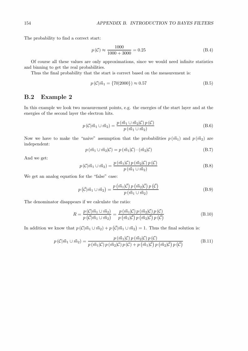
154 APPENDIX B. INTRODUCTION TO BAYES FILTERS
The probability to find a correct start:
p (C) ≈ 10001000 + 3000
= 0.25 (B.4)
Of course all these values are only approximations, since we would need infinite statisticsand binning to get the real probabilities.
Thus the final probability that the start is correct based on the measurement is:
p (C| m1 = {70|2000}) ≈ 0.57 (B.5)
B.2 Example 2
In this example we look two measurement points, e.g. the energies of the start layer and at theenergies of the second layer the electron hits.
p (C| m1 ∪ m2) =p ( m1 ∪ m2|C) p (C)
p ( m1 ∪ m2)(B.6)
Now we have to make the “naive” assumption that the probabilities p ( m1) and p ( m2) areindependent:
p ( m1 ∪ m2|C) = p ( m1|C) · ( m2|C) (B.7)
And we get:
p (C| m1 ∪ m2) =p ( m1|C) p ( m2|C) p (C)
p ( m1 ∪ m2)(B.8)
We get an analog equation for the “false” case:
p(C| m1 ∪ m2
)=
p( m1|C
)p( m2|C
)p(C)
p ( m1 ∪ m2)(B.9)
The denominator disappears if we calculate the ratio:
R =p (C| m1 ∪ m2)p(C| m1 ∪ m2
) =p ( m1|C) p ( m2|C) p (C)p( m1|C
)p( m2|C
)p(C) (B.10)
In addition we know that p (C| m1 ∪ m2) + p(C| m1 ∪ m2
)= 1. Thus the final solution is:
p (C| m1 ∪ m2) =p ( m1|C) p ( m2|C) p (C)
p ( m1|C) p ( m2|C) p (C) + p( m1|C
)p( m2|C
)p(C) (B.11)
Bibliography
Agaronian, F. A. and Sunyaev, R. A. ‘Gamma-ray line emission, nuclear destruction and neutronproduction in hot astrophysical plasmas - The deuterium boiler as a gamma-ray source.’Monthly Notices of the Royal Astronomical Society, 210: 257–277, 1984.
Agostinelli, S. et al. ‘Geant4 - A Simulation Toolkit.’ Nuclear Instruments and Methods A,(506): 250–303, 2003.
Ahn, K. and Komatsu, E. ‘Dark matter annihilation: The origin of cosmic gamma-ray back-ground at 1-20 MeV.’ Physical Review D, 72(6): 061301, 2005.
Andritschke, R. ‘Aufbau und Eichung der Kalorimeter fuer das Gammateleskop MEGA.’Diploma thesis, Technical University Munich, 2000. Available in German at the web-site:http://www.mpe.mpg.de/MEGA/mega-documents.html.
Andritschke, R. ‘Calibration of the MEGA Prototype.’ Ph.D. thesis, Technical UniversityMunich, Germany, 2006. To be published.
Aprile, E. et al. ‘Spectroscopy and Imaging Performance of the Liquid Xenon Gamma-RayImaging Telescope (LXeGRIT).’ Proc. SPIE, 4140, 2000.
Barrett, H. et al. ‘List-Mode likelihood.’ J. Opt. Soc. Am. A, 14(10), 1997.
Berger, M. and Seltzer, S. ‘Tables of Energy Losses and Ranges of Electrons and Positrons.’Technical Report NASA-SP-3012, NASA, 1964.
Bethe, H. A. ‘Molieres theory of multiple scattering.’ Physical Review, 89(6), 1953.
Bhattacharya, D. et al. ‘Prototype TIGRE Compton γ-ray balloon-borne instrument.’ NewAstronomy Reviews, 48: 287–292, 2004.
Bildsten, L. et al. ‘Helium destruction and gamma-ray line emission in accreting neutron stars.’The Astrophysical Journal, 408: 615–636, 1993.
Bloser, P. et al. ‘Development of Silicon Strip Detectors For a Medium Energy Gamma-raytelescope.’ NIM A, 512: 220–228, 2003.
Boehm, C. et al. ‘MeV Dark Matter: Has It Been Detected?’ Physical Review Letters, 92(10):101301, 2004.
Boggs, S. et al. ‘Overview of the nuclear Compton telescope.’ New Astronomy Reviews, 48:251–256, 2004.
Boggs, S. et al. ‘Report on the Advanced Compton Telescope vision mission study.’ Technicalreport, NASA, 2005. In press.
155

156 BIBLIOGRAPHY
Boggs, S. E. et al. ‘Event reconstruction in high resolution Compton telescopes.’ Astron.Astrophys. Suppl. Series, 145: 311–321, 2000a.
Boggs, S. E. et al. ‘Simulated Performance of a Germanium Compton Telescope.’ In Proceedingsof the 4th INTEGRAL Workshop, Alicante, Spain, 2000b.
Brun, R. and Rademakers, F. ‘ROOT - An Object Oriented Data Analysis Framework.’ NIMA, 389: 81–86, 1997. See also http://root.cern.ch/.
Caroli, E. et al. ‘Coded Aperture Imaging in X- and Gamma-Ray Astronomy.’ Space ScienceReviews, 45: 349–403, 1987.
CERN: Application Software Group and Networks Division. ‘Geant - Detector Description andSimulation Tool.’ Technical report, CERN Geneva, 1993.
Coburn, W. and Boggs, S. ‘Polarization of the prompt big gamma-ray emission from the biggamma-ray burst of 6 December 2002.’ Nature, 423: 415–417, 2003.
Compton, A. H. ‘A quantum theory of the scattering of X-ray by light elements.’ PhysicalReview, 21(5), 1923.
de Gouveia dal Pino, E. M. ‘Astrophysical jets and outflows.’ Advances in Space Research, 35:908–924, 2005.
Diehl, R. et al. ‘Astrophysical constraints from gamma-ray spectroscopy.’ Nuclear physics A,2005. In press.
DuMond, J. W. M. ‘Compton Modified Line Structure and its Relation to the Electron Theoryof Solid Bodies.’ Phys. Rev., 33: 643–658, 1929.
Dyks, J. et al. ‘Relativistic Effects and Polarization in Three High-Energy Pulsar Models.’ TheAstrophysical Journal, 606: 1125–1142, 2004.
Evans, R. The atomic nucleus. McGraw-Hill Book Company Inc., 1958.
Fichtel, C. et al. ‘High-Energy Gamma-ray Results from the Second Small Astronomy Satellite.’The Astrophysical Journal, 198: 163–182, 1975.
Forrest, D. J. et al. ‘The gamma ray spectrometer for the Solar Maximum Mission.’ SolarPhysics, 65: 15–23, 1980.
Gehrels, N. and other. ‘GLAST: the next-generation high energy gamma-ray astronomy mission.’Astroparticle Physics, 11(1): 277–282, 1999.
Gehrels, N. et al. ‘The SWIFT Gamma-Ray Burst Mission.’ The Astrophysical Journal, 611:1005–1020, 2004.
Georgii, R. et al. ‘COMPTEL upper limits for the 56Co γ-ray emission from SN1998bu.’ As-tronomy and Astrophysics, 394: 517–523, 2002.
Grindlay, J. et al. ‘EXIST: mission design concept and technology program.’ In Truemper, J. andTananbaum, H., editors, X-Ray and Gamma-Ray Telescopes and Instruments for Astronomy,volume 4851, pages 331–334. SPIE, 2003.
Halloin, H. ‘CLAIRE: Premieres Lumieres d’une Lentille Gamma.’ Ph.D. thesis, Universite PaulSabatier de Toulouse, 2003.

BIBLIOGRAPHY 157
Harris, M. J. et al. ‘Detection of γ-ray lines from interstellar 60Fe by the high resolutionspectrometer SPI.’ Astronomy and Astrophysics, 433: L49–L52, 2005.
Hernanz, M. ‘Classical nova explosions.’ In Hameury, J. and Lasota, J., editors, The Astrophysicsof Cataclysmic Variables and Related Objects. ASP Conference Series, 2004.
Hjorth, J. et al. ‘The optical afterglow of the short γ-ray burst GRB 050709.’ Nature, 437:859–861, 2005.
Hurford, G. et al. ‘The RHESSI Imaging Concept.’ Solar Physics, 210(1-2): 61 – 86, 2002.
Hurley, K. et al. ‘An exceptionally bright flare from SGR 1806-20 and the origins of short-duration big gamma-ray bursts.’ Nature, 434: 1098–1103, 2005.
Inoue, H. et al. ‘Astro-E2: the third X-ray observatory in the 21st Century.’ In Truemper, J. andTananbaum, H., editors, X-Ray and Gamma-Ray Telescopes and Instruments for Astronomy,volume 4851, pages 289–292. SPIE, 2003.
Iyudin, A. et al. ‘COMPTEL observations of Ti-44 gamma-ray line emission from CAS A.’Astronomy and Astrophysics, 284(1): L1–L4, 1994.
Iyudin, A. et al. ‘Resonant absorption troughs in gamma-ray spectra of QSO.’ Astronomy andAstrophysics, 436: 763–784, 2005.
Kanbach, G. et al. ‘The project EGRET (Energetic Gamma-Ray Experiment Telescope) onNASA’s Gamma-Ray Observatory (GRO).’ Space Science Reviews, 49: 69–84, 1988.
Kanbach, G. et al. ‘Development and calibration of the tracking Compton/Pair telescopeMEGA.’ Nuclear Instruments and Methods in Physics Research A, 541: 310–322, 2005.
Kippen, R. ‘The GEANT low energy Compton scattering (GLECS) package for use in simulatingadvanced Compton telescopes.’ New Astronomy Reviews, 48: 221–226, 2004.
Klein, O. and Nishina, T. ‘Uber die Streuung von Strahlung durch freie Elektronen nachder neuen relativistischen Quantendynamik von Dirac.’ The European Physical Journal A- Hadrons and Nuclei (Historical Archive), 52(11-12): 853–868, 1929.
Knodelseder, J. ‘Prospects in space-based gamma-ray astronomy.’ In Favata, F. and Gimenez,A., editors, Proc. 39th ESLAB Symposium, 2005.
Knodelseder, J. et al. ‘The all-sky distribution of 511 keV electron-positron annihilation emis-sion.’ Astronomy and Astrophysics, 441: 513–532, 2005.
Kurfess, J. et al. ‘An advanced Compton telescope based on thick, position-sensitive solid-statedetectors.’ New Astronomy Reviews, 48: 293–298, 2004.
Lange, K. and Carson, R. ‘EM reconstruction algorithms for emission and transmission tomog-raphy.’ Journal of Computer Assisted Tomography, 8(2): 306–316, 1984.
Lebrun, F. et al. ‘Compact sources as the origin of the soft γ-ray emission of the Milky Way.’Nature, 428: 293–296, 2004.
Lei, F. et al. ‘Compton scatter polarimetry in gamma-ray astronomy.’ Space Sci. Rev., 82:309–388, 1997.
Leibundgut, B. ‘Type Ia Supernovae.’ The Astron Astrophys Rev, 10: 179–209, 2000.

158 BIBLIOGRAPHY
Lin, R. et al. ‘The Reuven-Ramaty High-Energy Solar Spectroscopic Imager (RHESSI).’ SolarPhysics, 219: 3–32, 2002.
Litvinenko, V. et al. ‘High power inverse Compton gamma-ray source at Duke storage ring.’SPIE, 2521: 55–77, 1995.
Litvinenko, V. et al. ‘Gamma-Ray production in a storage Ring Free-Electron Laser.’ PhysicalReview Letters, 78(24): 4569–4572, 1997.
Lucy, L. B. ‘An iterative technique for the rectification of observed distributions.’ The Astro-nomical Journal, 79: 745–754, 1974.
Massaglia, S. ‘Constraining the parameters of AGN jets.’ Astrophysics and Space Science, 287:223–233, 2003.
McConnell, M. et al. ‘COMPTEL All-Sky Imaging at 2.2 MeV.’ In AIP Conf. Proc. 410:Proceedings of the Fourth Compton Symposium, page 1099, 1997.
Milne, P. et al. ‘Advanced Compton Telescope designs and SN science.’ New Astronomy Reviews,48: 617–623, 2002.
Modesitt, G. and Koch, H. ‘Nuclear Impulse in Electron Pair Creation.’ Physical Review, 77(2):175–179, 1950.
Morris, D. J. et al. ‘Evidence for 56Co Line Emission from the Type Ia Supernova 1991 T UsingCOMPTEL.’ In Seventeenth Texas Symposium on Relativistic Astrophysics and Cosmology,pages 397–400, 1995.
Mowlavi, N. et al. ‘Search for 26Al in Gamma Velorum.’ In Schoenfelder, V., Lichti, G., andWinkler, C., editors, ESA SP-552: 5th INTEGRAL Workshop on the INTEGRAL Universe,2004.
Nefzger, C. ‘Entwicklung von Methoden zur Auswertung von Einzel-Ereignissen des neuartigenGamma-Teleskops MEGA.’ Diploma thesis, Technical University Munich, 2000. Available inGerman at the web-site: http://www.mpe.mpg.de/MEGA/mega-documents.html.
Oberlack, U. et al. ‘COMPTEL limits on 26Al 1.809 MeV line emission from gamma2 Velorum.’Astronomy and Astrophysics, 353: 715–721, 2000a.
Oberlack, U. et al. ‘A Compton scattering sequence reconstruction algorithm for the liquidxenon gamma-ray imaging telescope (LXeGRIT).’ In R.B. James, R. S., editor, Hard X-Ray,Gamma-Ray, and Neutron Detector Physics II, volume 4141, pages 168–177. SPIE, 2000b.
O’Neill, T. J. ‘Tracking, Imaging, and Polarimeter Properties of the TIGRE Instrument.’ As-tronomy and Astrophysics Supplement Series, 120, 1996.
Owens, A. et al. ‘The Transient Gamma-Ray Spectrometer.’ IEEE Transactions on NuclearScience, 39(2): 559–567, 1991.
Palacios, A. et al. ‘New estimates of the contribution of Wolf-Rayet stellar winds to the Galactic26Al.’ Astronomy and Astrophysics, 429: 613–624, 2005.
Park, S. H. et al. ‘Spatial distribution and polarization of γ-rays generated via Comptonbackscattering in the Duke/OK-4 storage ring FEL.’ Nuclear Instruments and Methods inPhysics Research A, 475: 425–431, 2001.
BIBLIOGRAPHY 159
Particle Data Group. ‘Review of Particle Physics.’ Physics Letters B, 592(1-4), 2004.
Pluschke, S. ‘26Al Ursprung und OB-Assoziationen.’ Ph.D. thesis, Technische UniversitatMunchen, 2001.
Prantzos, N. ‘Radioactive 26Al and 60Fe in the Milky Way: implications of the RHESSI detectionof 60Fe.’ Astronomy and Astrophysics, 420: 1033–1037, 2004.
Press, W. Numerical recipes in C: the art of science computing. Cambridge, 1992.
Ramaty, R., Kozlovsky, B., and Lingenfelter, R. ‘Nuclear Gamma-Ray From Energetic ParticleInteractions.’ The Astrophysical Journal Supplement Series, 40: 487–526, 1979.
Renaud, M. et al. ‘An INTEGRAL/IBIS view of Young Galactic SNRs through the 44Ti gamma-ray lines.’ New Astronomy Reviews, 2005. In preparation.
Ribberfors, R. ‘Relationship of the relativistic Compton cross section to the momentum distri-bution of bound electron states. II. Effects of anisotropy and polarization.’ Physical ReviewB, 12: 3136–3141, 1975.
Ribberfors, R. and Berggren, K.-F. ‘Incoherent-X-ray-scattering functions and cross sections bymeans of a pocket calculator.’ Physical Review A, 26: 3325–3333, 1982.
Richardson, W. H. ‘Bayesian-based iterative method of image restoration.’ Optical Society ofAmerica Journal A, 1972.
Riess, A. et al. ‘Observational Evidence from Supernovae for an Accelerating Universe and aCosmological Constant.’ The Astronomical Journal, 116: 1009–1038, 1998.
Schaefer, B. E. et al. ‘High-energy spectral breaks in gamma-ray bursts.’ The AstrophysicalJournal, 393: L51–L54, 1992.
Schmid, G. J. et al. ‘A γ-ray tracking algorithm for the GRETA spectronometer.’ NIM A, 430:69–83, 1999.
Schonfelder, V. et al. ‘Instrument description and performance of the imaging gamma-raytelescope COMPTEL aboard the Compton Gamma-Ray Observatory.’ The AstrophysicalJournal Supplement Series, 86: 657–692, 1993.
Schonfelder, V. et al. ‘The first COMPTEL source catalogue.’ Astronomy and AstrophysicsSupplement, 143: 145–179, 2000.
Schonfelder, V. et al. ‘Ti-44 Gamma-Ray Line Emission from Cas A and RXJ0852-4622/GROJ0852-4642.’ In McConnell, M. and Ryan, J., editors, The Fifth Compton Sympo-sium, volume 510. AIP Conference Proceedings, 2000.
Schopper, F. ‘Entwicklung eines Teleskops zur Abbildung von Gammastrahlung mittels Comp-tonstoß und Paarerzeugung.’ Ph.D. thesis, Technical University Munich, Germany, 2001.
Sizun, P. et al. ‘The INTEGRAL/SPI Response and the Crab Observations.’ In ESA SP-552:5th INTEGRAL Workshop on the INTEGRAL Universe, pages 815–818, 2004.
Skinner, G. ‘Diffractive/refractive optics for high energy astronomy: I. Gamma-ray phase Fresnellenses.’ Astronomy & Astrophysics, 375: 691–700, 2001.
Smith, D. M. ‘Gamma-Ray Line Observations with RHESSI.’ In ESA SP-552: 5th INTEGRALWorkshop on the INTEGRAL Universe, pages 45–48, 2004.

160 BIBLIOGRAPHY
Stanek, K. et al. ‘Spectroscopic discovery of the supernova 2003dh associated with GRB 030329.’The Astrophysical Journal, 591: L17–L20, 2003.
Stecker, F. and Salamon, M. ‘The Extragalactic Gamma-Ray Background.’ In Ritz, S., Gehrels,N., and Shrader, C., editors, Gamma-ray Astrophysics, pages 432–441. AIP, New York, 2001.
Strigari, L. et al. ‘The concordance cosmic star formation rate: implications from and for thesupernova neutrino and gamma ray backgrounds.’ Journal of Cosmology and AstroparticlePhysics, 2005.
Strong, A. W. et al. ‘A New Determination Of The Diffuse Galactic and Extragalactic Gamma-Ray Emission.’ In AIP Conf. Proc. 745: High Energy Gamma-Ray Astronomy, pages 585–590,2005.
Tavani, M. et al. ‘The AGILE instrument.’ In Truemper, J. and Tananbaum, H., editors, X-Rayand Gamma-Ray Telescopes and Instruments for Astronomy, volume 4851, pages 1151–1162.SPIE, 2003.
Thompson, D. J. et al. ‘Calibration of the Energetic Gamma-Ray Experiment Telescope(EGRET) for the Compton Gamma-Ray Observatory.’ The Astrophysical Journal Supple-ment Series, 86: 629–656, 1993.
van der Marel, J. and Cederwall, B. ‘Backtracking as a way to reconstruct Compton scatteredγ-rays.’ NIM A, 437: 538–551, 1999.
von Ballmoos, P. et al. ‘The MAX Mission: Focusing on High-Sensitivity Gamma-Ray Spec-troscopy.’ In ESA SP-552: 5th INTEGRAL Workshop on the INTEGRAL Universe, pages747–750, 2004.
Watanabe, K. and Hartmann, D. ‘Contributions of GRBs and Cen A-like Radio Galaxies tothe Cosmic Gamma-ray Background.’ In Ritz, S., Gehrels, N., and Shrader, C., editors,Gamma-ray Astrophysics, pages 442–445. AIP, New York, 2001.
Weidenspointner, G. et al. ‘MGGPOD: a Monte Carlo Suite for Modeling Instrumental Line andContinuum Backgrounds in Gamma-Ray Astronomy.’ The Astrophysical Journal SupplementSeries, 156: 69–91, 2005.
Wigger, C. et al. ‘Can RHESSI be used as GRB Polarimeter?’ In Schoenfelder, V., Lichti,G., and Winkler, C., editors, ESA SP-552: 5th INTEGRAL Workshop on the INTEGRALUniverse, 2004.
Wilderman, S. et al. ‘List-mode Maximum Likelihood Reconstruction of Compton Scatter Cam-era Images in Nuclear Medicine.’ IEEE Trans. Nucl. Sci., 45: 957, 1998.
Winkler, C. et al. ‘The INTEGRAL mission.’ Astronomy and Astrophysics, 411: L1–L6, 2003.
Wolter, D. et al. ‘MEGA Pre-Phase A Study.’ Technical report, DaimlerCrysler Aerospace,Jena-Optronik GmbH, 2000.
Wunderer, C. et al. ‘The ACT Vision Mission Study Simulation Effort.’ New Astronomy Reviews,2006. In press.
Zoglauer, A. ‘Methoden der Bildrekonstruktion fuer das Comptonteleskop MEGA.’ Diplomathesis, Technical University Munich, 2000. Available in German at the web-site:http://www.mpe.mpg.de/MEGA/mega-documents.html.

Acknowledgments
This work would not have been possible without the support and contributions of numerousothers, and I would like to express my sincere gratitude to all of them:
• Prof. Volker Schonfelder for providing me the opportunity to work on such an interestingbut sometimes really challenging topic, and for his continued interest in the completion ofthis work.
• Gottfried Kanbach, my advisor, for all his guidance, his support and all the fruitful dis-cussions, for proof-reading many manuscripts, for his readiness to accept telephone callson weekends and late at night, for giving me the opportunity to present my work at in-ternational meetings, and of course for his unbreakable enthusiasm for MEGA even whenthe detector didn’t want to run at all.
• Robert Andritschke for getting the MEGA job done, for providing the excellent calibrationof the prototype, which took him a year of 36-hour days, for his patience with MEGA (andnot making good on his threats to throw the prototype out of the window), for his excellentskills in electronics, without which MEGA probably would have measured only randomnoise, for his friendship since the first day when we both started studying physics, for ...ok if I would list everything he has done for MEGA, then this text would go on for a while... he was the real MEGA-man during the last five years!
• Trixi Wunderer for cheering me up during the darkest moments of the MEGA data analysis,for seeing the MEGA performance in much more positive light than I would ever be ableto, for her excellent and elaborate proofreading of this work, for taking care of my well-being especially at the end phase of this work, and finally for hiding all the Easter eggs —which MEGA all found!
• Florian Schopper for laying the ground for the MEGA prototype, inspiring me to use list-mode as the image reconstruction algorithm of choice for MEGA, and introducing me toMEGA with one of the shortest job interviews ever (“Kannst du programmieren?”).
• Fritz Schrey for taking care of numerous smaller and larger problems of the MEGA me-chanics and electronics and organizing the logistics of the Duke campaign, for making surethat we all got our daily lunch at noon sharp (“Geh’ma jetzt endlich essen!?”) — and ofcourse for the propeller, which enabled the “supernova remnant” measurement!
• Peter Bloser for numerous helpful discussions on polarization and pair production and hissupport during all the calibrations of the MEGA prototype.
• Werner Collmar for introducing me to COMPASS, for providing me with COMPTEL data,and of course for an apartment in Garching really close to MPE.
• Karsten Kretschmer, Alexander Stefanescu and Christian Clemens for all the fruitful dis-cussions about Linux, Bash, physics, astronomy, etc.
161

• Vladimir Litvineko and his crew at HIGS, for providing the excellent calibration beam;thanks also to all others who helped during the Duke campaign.
• Georg Weidenspointer and Steve Sturner for implementing the ACT/MEGAlib extensioninto MGeant/MGGPOD, which enabled the orbital background simulations for MEGA.
• Steve Boggs for giving me the opportunity to finish this thesis at the Space Science Lab-oratory in Berkeley, California — long after MPE stopped its financial support, and toJason Bowen and Mark Bandstra for some helpful discussions.
And of course a big thank you to all who helped to get MEGA up and running at MPE andto all the other gamma-ray astronomers at MPE and SSL for their support during this workand for providing the excellent work atmosphere at both places.
Above all my very special thanks goes to my parents and grandparents — without theircontinuing support this work would have never been possible!
Thank you — Dankeschon!