INTRODUCTION This document is intended for use with “Keeping the books for environmental systems: An Emergy Analysis of West Virginia” by Daniel Campbell, Maria Meisch, Tom DeMoss, John Pomponio, and Patricia Bradley published in Environmental Monitoring and Assessment Volume 94: 217-230, 2004 (Campbell et al. 2004). It is described in that article as supporting data and materials residing at http://www.epa.gov/aed/research/desupp3.html. The references, data sources, and append ices given in this document will be part of a USEPA research report titled “Environmental Accounting Using Emergy: Evaluation of the State of West Virginia” by D.E. Campbell, S.L. Brandt-Williams, and M. E.A. Meisch that will be published later this year (2004). The data, sources, and calculations used to obtain the numbers found in Campbell et al. (2004) are given in the appendices that follow. In the intervening year between completion of Campbell et al. (2004) and the completion of the aforementioned USEPA Research Report errors were corrected and calculations were refined; therefore, some of the numbers in the technical report and on this web site are different from the numbers in Campbell et al. (2004). A list of the major changes follows: (1) In the calculations in Campbell et al. (2004) a transformity of 196,000 sej/J was used for electricity and 156,000 sej/J for hydroelectricity these values have been replaced using broader averages from Odum (1996) and are now 170,400 for electricity and 120,300 sej/J for hydroelectricity. To obtain these averages adjust the values in Odum (1996) to the 9.26 E+24 sej/y planetary baseline. As a result all numbers that depended on the emergy of electricity used or exported are somewhat different here than in Campbell et al. 2004. (2) The 1997 emergy to dollar ratio for the United States was recalculated and found to be 1.20 x 1012 sej/$ rather than 1.22 x 1012 sej/$. This change was due to the lower transformity of electricity used to estimate nuclear energy’s emergy contribution to the emergy resource base for the United States. The transformity of coal electricity was used to estimate the emergy contribution of nuclear electricity. As a result of the change in the emergy to money ratio for 1997, all the estimates of emdollar values given in Campbell et al. (2004) must be multiplied by 1.01667 to obtain the numbers in this posting given that no other factor has intervened to cause a change in the emergy estimate for an item. (3) The geopotenial energy in runoff absorbed in the state was incorrectly calculated in Campbell et al. (2004), because the energy absorbed was determined relative to sea level rather than to the lowest point where the river water leaves the state. When this error was corrected the geopotential emergy absorbed decreased from 18 E+20 sej/y to 16 E+20 sej/y. (4) The transformity of agricultural products in this posting was determined using a weighted average based on mass. The greater mass of hay lowers the overall transformity from that used in Campbell et al. (2004). (5)The factor 2:1 used to estimate raw material for the aluminum industry was based on alumina. In fact the estimate should have been 4:1 for bauxite. The correction is made in these tables. (6) The rule used to estimate imported service was changed. The ratio of the state’s per capita income to the national average per capita income was used to estimate the quantity of potentially imported services that would probably be imported when a state’s per capita income is less than the national average. As a result our estimate of West Virginia’s imported services increased from 4 billion to 6.2 billion dollars. (7)As a result of the previous changes the emergy to dollar ratio for West Virginia changed very slightly from 5.72 to 5.78 E+12 sej /$.

(8) Tourism should have been an entry on the exports table rather than the imports table. It is entered this way in the technical report. (9) Slight changes in the numbers in the summary and indices tables follow as a consequence of these changes. (10) The conclusions and relationships in Campbell et al. (2004) remain unchanged by the corrections made to the analysis as a result of further examination and criticism over the past year. The above list of changes may not be exhaustive since there are many possibilities for miscalculations and errors in such a large analysis. If any visitor to this site finds an error in or has a question about the information posted here they may contact me at Campbell.dan@epa.gov.

REFERENCES

Adams, M.B., Kochenderfer, J.N., Wood, F., Angradi, T.R., Edwards, P. 1993. Forty Years of Hydrometeorological Data from the Fernow Experimental Forest, West Virginia. United States Department of Agriculture, Forest Service, Northeastern Forest Experiment Station, General Technical Report NE-184. 24 p.

Arnold, J.G., Williams, J.R. 1985. Evapotranspiration in a Basin Scale Hydrologic Model, pp.

405-413. In: Advances in Evapotranspiration, Proceedings of the National Conference on Advances in Transpiration, American Society of Agricultural Engineers, St. Joseph, MI.

Brandt-Williams, S., 1999. Evaluation of Watershed Control of Two Central Florida Lakes:

Newnans Lake and Lake Weir. Ph.D. dissertation, University of Florida, 257pp. Brandt-Williams, S.L. 2001 (revised 2002). Handbook of Emergy Evaluation. Folio #4. Emergy

of Florida Agriculture. Center for Environmental Policy, Environmental Engineering Sciences, University of Florida, Gainesville, FL. 40 p.

Brown, M.T., Buranakarn, V. 2000. Emergy Evaluation of Material Cycles and Recycle Options, pg 141-154, In Brown, M.T., (ed) Emergy Synthesis, Proceedings of the First Biennial Emergy Analysis Research Conference, The Center for Environmental Policy, Department of Environmental Engineering Sciences, University of Florida, Gainesville, FL.

Brown, M.T. and Ulgiati, S.: 2001, ‘Emergy measures of carrying capacity to evaluate economic

investments, Population and Environment 22, 471-501 Brown, M.T., Woithe, R.D., Odum, H.T., Montague, C.L., Odum, E.C. 1993. Emergy

Analysis Perspectives on the Exxon Valdez Oil Spill in Prince William Sound, Alaska. Report to the Cousteau Society, Center for Wetlands and Water Resources, CWWR 93-1, University of Florida, Gainesville.

Buranakarn, V. 1998. Evaluation of Recycling and Reuse of Building Materials Using the

Emergy Analysis Method. PhD. Dissertation, University of Florida, UMI Dissertation Services, Ann Arbor MI, 257 p.

Campbell, C.J., Laherrere, J.H. 1998. The End of Cheap Oil. Scientific American (March): 78-83.

Campbell, D.E. 1998. Emergy Analysis of Human Carrying Capacity and Regional

Sustainability: An Example Using the State of Maine. Environmental Monitoring and Assessment 51:531-569.

Campbell, D E., 2000a. A revised solar transformity for tidal energy received by the earth and dissipated globally: Implications for Emergy Analysis, pp. 255-264. In M.T. Brown (ed) Emergy Synthesis: Theory and applications of the Emergy methodology. Proceedings of the 1st Biennial Emergy Analysis Research Conference, Center for Environmental Policy, Department of environmental Engineering Sciences, University of Florida, Gainesville, FL.

Campbell, D.E. 2000b. Using energy systems theory to define, measure, and interpret ecological

integrity and ecosystem health. Ecosystem Health 6(3):181-204.

Campbell, D.E. 2003. A Note on the Uncertainty in Estimates of Transformities Based on Global Water Budgets, pp. 349-353. In Brown, M.T., Odum, H.T., Tilley, D.R., Ulgiati, S. (eds.) Emergy Synthesis 2. Proceedings of the Second Biennial Emergy Analysis Conference. Center for Environmental Policy, University of Florida, Gainesville.

Campbell, D.E., 2004. Financial Accounting Methods to Further Develop and Communicate

Environmental Accounting Using Emergy , pp. ?-?. In Brown, M.T. (ed). Emergy Synthesis 3. Proceedings of the Third Biennial Emergy Analysis Conference, Center for Environmental Policy, University of Florida, Gainesville.

Campbell, D., Meisch M., DeMoss, T., Pomponio, J., Bradley, P. 2004a. Keeping the books for

the environment: An emergy analysis of West Virginia. Environmental Monitoring and Assessment 94: 217-230.

Campbell, D.E., Brandt-Williams, S.L., Cai, T.T. 2004b. Current Technical Problems in Emergy

Analysis. pp. ?-?. In Brown, M.T. (ed). Emergy Synthesis 3. Proceedings of the Third Biennial Emergy Analysis Conference, Center for Environmental Policy, University of Florida, Gainesville.

Canaan Valley Institute (CVI),: 2002, Mid-Atlantic Highlands Action Plan, Transforming the

Legacy, Canaan Valley Institute, Thomas, WV.

Clarkson, R.B. 1964. Tumult on the Mountains: Lumbering in West Virginia � 1770 - 1920. McLain Printing Company, Parsons, West Virginia.

Degens, E.T. 1965. Geochemistry of Sediments, A Brief Survey. Prentice-Hall, Englewood Cliffs,

NJ. 342 p. DiGiovanni, D.M. 1990. Forest Statistics for West Virginia – 1975 and 1989. United States

Department of Agriculture, Forest Service, Northeastern Forest Experiment Station, Resource Bulletin NE-114. 28 p.

Finkel, A.M. 1990. Confronting Uncertainty in Risk Management. Center for Risk Management,

Resources for the Future. Washington, D.C. 69 pp. Krug, W.R., Gebert, W.A., Craczyk, Stevens, D.J., Rochelle, B.P., Church, M.R., 1990. Map of

mean annual runoff from the northeastern, southeastern, and mid Atlantic United States, water years1951-1980, United States Geological Survey, WRI 88-4094. 11p.

Lotka, A.J. 1922. Contribution on the energetics of evolution. Proc. Natl. Acad. Sci. 8, 147-151. Martinez-Alier, J.: 1987, Ecological Economics, Basil Blackwell, N.Y. 286 pp. Miller, B.I.: 1964, A Study of the Filling of Hurricane Donna Over Land (1960). Mon. Wealth.

Rev. U.S. Dept. of Ag. 92 (9), p. 389-406. National Energy Policy Development Group, National Energy Policy, US Government

Printing Office, Washington, D.C., 2001, pg 1-1.

National Research Council, Our Common Journey, a transition toward sustainability, National Academy Press, Washington, D.C., 1999, pg. 14.

Odum, H.T.: 1988, ‘Self-organization, transformity, and information’. Science 242, 1132-1139. Odum, H.T.: 1994, Ecological and General Systems. University Press of Colorado, Niwot, CO.

644 pp. (reprint of Systems Ecology, John Wiley, 1983)

Odum, H.T.: 1996, Environmental Accounting: Emergy and Environmental Decision Making; John Wiley and Sons, NY.

Odum, H.T. 1999. "Evaluating Landscape Use of Wind Kinetic Energy". Unpublished manuscript.

Odum, H.T. 2000. Handbook of Emergy Evaluation. Folio #2. Emergy of Global Processes. Center for Environmental Policy, Environmental Engineering Sciences, University of Florida, Gainesville, FL. 30 p.

Odum, H.T., Arding, J. E. (1991) EMERGY Analysis of Shrimp Mariculture in Ecuador. Report to Coastal Resource Center, University of Rhode Island, Center for Wetlands, Univ. of Florida, Gainesville, FL, 87 p.

Odum, H.T., Odum, E.C. 2000. Modeling for All Scales. Academic Press, San Diego, CA. 458 p. Odum, H.T., Odum, E.C., 2001. A Prosperous Way Down. University Press of Colorado,

Boulder, CO. 326 p. Odum, H.T., Brown, M.T., Christianson, R.A. 1986b. Energy Systems Overview of the Amazon

Basin. Report to the Cousteau Society, Center for Wetlands, CFW Publication # 86-1, University of Florida, Gainesville, FL. 190 p.

Odum, H.T., Odum, E.C., Blissett, M.: 1987, The Texas System, Emergy Analysis and

Public Policy. A Special Project Report, L.B. Johnson School of Public Affairs. University of Texas at Austin, and The Office of Natural Resources, Texas Department of Agriculture, Austin.

Odum, H.T., Romitelli, S., Tigne, R. 1998a. Evaluation Overview of the Cache River and Black Swamp in Arkansas. Center for Environmental Policy, Environmental Engineering Sciences, University of Florida, Gainesville, FL, 1998.

Odum, H.T., Odum, E.C., Brown, M.T. 1998b. Environment and Society in Florida. St. Lucie

Press, Boca Raton, FL. 449 pp. Odum, H.T., Brown, M.T., Brandt-Williams, S.L. 2000a. Handbook of Emergy Evaluation. Folio

#1. Introduction and Global Budget. Center for Environmental Policy, Environmental Engineering Sciences, University of Florida, Gainesville, FL. 16 p.

Odum, H.T. Kemp, W., Sell, M., Boynton, W., Lehman, M. 1977. Energy analysis and the

coupling of man and estuaries. Environmental Management 1(4): 297-315. Odum, H.T., Odum, E.C., Brown, M.T., Scott, G.B., Lahart, D., Bersok, C., Sendzimir,

J.: 1986a. Florida Systems and Environment.; A supplement to the test Energy Systems and Environment. University of Florida, Center for Wetlands.

Odum, H.T., Wojcik,W., Pritchard, L., Ton, S., Delfino, J.J., Wojcik, M. Leszczynski, S. Patel, J.D., Doherty, S.J., Stasik, J. 2000b. Heavy Metals in the Environment, Using Wetlands for Their Removal. CRC Press LLC, Lewis Publishers, Boca Raton, FL. 325 p.

Patric, J. H.,Evans, J.O., Helvey, J.D. 1984. Summary of Sediment Yield Data From Forested Land in the United States, Journal of Forestry 82: 101-104.

Reiter, E.R. 1969. Atmospheric Transport processes, Part I. Energy Transfers and Transformations. U.S. Atomic Energy Commission, Division of Technical Information, Oak Ridge, TN. 253 p.

Rice, O.K. 1985. West Virginia: A History, University Press, of Kentucky, Lexington, KY Rice, O.K. and Brown, S.W.: 1993, West Virginia: A History, 2nd Ed, University Press of

Kentucky, Lexington. Romitelli, M. S. 1997. Energy Analysis of Watersheds. PhD. Dissertation, University of Florida,

UMI Dissertation Services, Ann Arbor, MI. 292 p. Rosler, H.J., Lange, H. 1972. Geochemical Tables. Elsevier Publishing Company, Amsterdam.

468 p. Scatena, F.N.,Doherty, S.J., Odum, H.T., Kharecha, P. 2002. An Emergy Evaluation of Puerto

Rico and the Luquillo Experimental Forest. U.S. Department of Agriculture, Forest Service, International Institute of Tropical Forestry, General Technical Report IITF-GTR-9, Rio Piedras, PR. 79 p.

State of West Virginia , 1935. West Virginia Blue Book, State Legisla tive Manual, Charleston,

WV. State of West Virginia, 1999. West Virginia Blue Book, Charleston, WV.

Tilley, D.R., 1999. Emergy Basis of Forest Systems, PhD. Dissertation, University of Florida,

UMI Dissertation Services, Ann Arbor MI, 296 p.

Ulgiati, S., Odum, H.T., Bastianoni, S. 1994. Emergy use, environmental loading and sustainability: An emergy analysis of Italy. Ecological Modelling 73: 215-268.

Warren, Greg. Pers. Comm. Weirton Steel, Wheeling, WV.

DATA SOURCES (1) USDA Nutrient Data Laboratory “Food Composition and Nutrition.” http://www.nal.usda.gov/fnic/cgi-bin/nut_search.pl (2) U.S. Census, Commodity Flow Survey for 1997. http://www.census.gov/econ/www/cdstate.html (3) http://www.eia.doe.gov (4) http://dataweb.usitc.gov/scripts/user_set.asp (5)http://www.eia.doe.gov/pub/oil_gas/natural_gas/data_publications/natural_gas_annual/historical/1997/nga_1997.html (6) http://tonto.eia.doe.gov/FTPROOT/coal/058497.pdf (7) http://garnet.acns.fsu.edu/~tchapin/urp5261/topics/econbase.htm (8) http://www.nylovesbiz.com/nysdc/Personalincome/stpcpi9702.pdf (9) http://www.ers.usda.gov/StateFacts/WV.HTM (10) http://eosweb.larc.nasa.gov/cgi-bin/sse/register.cgi?task=login&next_url=/cgi-bin/sse/ion-p&page=globe_main.ion&app=sse (11) University of Utah. “Average Wind Speed (mph).”Meteorological Department. 1993. http://www.met.utah.edu/jhorel/html/wx/climate/windavg.html (7 June 1997). (12) International Heat Flow Commission, “Global Heat Flow Database”, University of North Dakota. http://heatflow.und.nodak.edu/index2.html (17 May 2002). (13) West Virginia Blue Book, 1999. Charleston, WV. (14) Direct measurements of forest evapotranspiration in West Virginia are found at http://www.esd.ornl.gov/programs/WBW/D1998.HTM (15) West Virginia Blue Book, 1999. Charleston, WV and Krug, et al. (1990). (16) Water quality data for the rivers from the USGS water resources website. New River Glen Lyn, VA http://waterdata.usgs.gov/va/nwis/qwdata?qw_count_nu=1&parameter_cd=00095&begin_date=&end_date=&format=html_table&site_no=03176500&agency_cd=USGS For the Ohio River at Sewickley, PA: http://waterdata.usgs.gov/pa/nwis/qwdata?qw_count_nu=1&parameter_cd=00095&begin_date=&end_date=&format=html_table&site_no=03086000&agency_cd=USGS Point Pleasant WV: http://waterdata.usgs.gov/wv/nwis/qwdata?site_no=03201500&agency_cd=USGS&begin_date=&end_date=&format=html_table&pre_format=on&inventory_output=0&rdb_inventory_output=file&date_format=YYYY-MM-DD&rdb_compression=file&qw_sample_wide=0&submitted_form=brief_list (17) The New River at Glen Lyn VA: http://waterdata.usgs.gov/va/nwis/annual/calendar_year?site_no=03176500&agency_cd=USGS&format=html The Ohio River at Sewickley, PA> http://waterdata.usgs.gov/pa/nwis/annual/calendar_year?site_no=03086000&agency_cd=USGS&format=html The Ohio River at Point Pleasant, WV: http://waterdata.usgs.gov/wv/nwis/annual/calendar_year/?site_no=03201500 (18) U.S. Department of Agriculture “1997 Census of Agriculture, Vol. 1, Part 48, Chapter 1.” http://www.nass.usda.gov/census/census97/volume1/wv-48/toc97.htm (29 April 1999).

West Virginia Agricultural Statistics Service, “2001 West Virginia Agricultural Statistics.” http://www.nass.usda.gov/wv/page1.pdf (7 Sept. 2001). A general source for all states in 1997 is http://www.nass.usda.gov/census/census97/volume1/vol1pubs.htm and also http://www.usda.gov/nass/sso-rpts.htm (19) US Dept of Agriculture 1998 Census of Aquaculture - Table 9 http://www.nass.usda.gov/census/census97/aquaculture/aquaculture.htm (20) Electricity Net Generation http://www.eia.doe.gov/cneaf/coal/statepro/imagemap/wv2p1.html (21) Forestry Service “West Virginia 1989 Forest Inventory.” (13 July 2000). http://www.fs.fed.us/ne/fia/states/wv/wvhilite.html A general source for U.S. timber statistics found at the following web address: http://www.fpl.fs.fed.us/documnts/fplrp/fplrp595.pdf Also useful are Alabama Forestry Commission, “Southern Wood Conversion Factors and Rules of Thumb” http://members.aol.com/JOSTNIX/convert.htm (19 Aug. 1997) and Cooperative Extension Institute of Agriculture and Natural Resources “Specie s Characteristics and Volumes.” University of Nebraska http://www.ianr.unl.edu/pubs/forestry/g881.htm (14 April 2000). (22) U.S. Geological Survey, “National Water-Use data files.” http://water.usgs.gov/watuse/spread95/wvco95.txt (9 July 2001). (23) West Virginia Department of Energy, “West Virginia Coal Statistics” http://www.eia.doe.gov/cneaf/coal/statepro/imagemap/wv1p1.html (30 Oct. 2001). (24) U.S. Census Bureau Conversion Tables http://www.census.gov/foreign-trade/www/sec9.html (25) Energy Information Administration, “Natural Gas Production and Consumption for 1999.” http://www.eia.doe.gov/pub/oil_gas/natural_gas/data_publications/natural_gas_annual/current/pdf/table_090.pdf (19 Nov. 2001). (26) Utah's Department of Natural Resources - Energy Office http://www.nr.utah.gov/energy/pub/stab99/chap8.pdf (27) U.S. Energy Information Association Energy Consumption Estimates by Source, 1960-1999 http://www.eia.doe.gov/pub/state.data/pdf/wv.pdf and Energy Information Administration, “West Virginia State Energy Production and Consumption for 1999.” http://www.eia.doe.gov/emeu/states/_statequads.html (29 June 2001). (28) Electricity Net Generation http://www.eia.doe.gov/cneaf/coal/statepro/imagemap/wv2p1.html (29) US Geological Survey and the West Virginia Geological and Economic Survey, “2000 Mineral Industry Study of West Virginia.” http://minerals.usgs.gov/minerals/pubs/state/985401.pdf (13 Dec. 2001). (30) 1997 West Virginia Erosion Estimates. http://www.wv.nrcs.usda.gov/nri/erosionwater.htm (31) 1997 Economic Census: Summary Statistics for West Virginia, http://www.census.gov/epcd/ec97/wv/WV000.HTM and Summary Statistics for the U.S. http://www.census.gov/epcd/ec97/us/US000.HTM and by industry http://www.census.gov/epcd/ec97/industry/E3331.HTM (32) West Virginia Department of Transportation http://www.wvcorridorh.com/economic/tourism.html (11 Feb. 2002). (33) Federal Funds - Summary Distribution by State (1996) http://www.census.gov/prod/3/98pubs/98statab/sasec10.pdf (34) West Virginia Coal Reserves http://www.state.wv.us/mhst/reserves98.pdf

(35) Petroleum Profile of West Virginia, United States Energy Information Association http://tonto.eia.doe.gov/oog/info/state/wv.asp (36) Average price of Bauxite http://minerals.usgs.gov/minerals/pubs/commodity/bauxite/090398.pdf Average price of Coal http://www.eia.doe.gov/cneaf/coal/cia/html/t80p01p1.html Petroleum Price http://www.eia.doe.gov/emeu/states/oilprices/oilprices_wv.html Iron Ore Price http://www.indiainfoline.com/sect/iror/db01.html Aluminum Price http://www.amm.com/ref/alum.HTM (37) For states with an international port of entry data on imports can be found at http://www.ustr.gov/outreach/states/westva.pdf Office of the United States Trade Representative. Also see http://dataweb.usitc.gov/scripts/user_set.asp for West Virginia Exports (38) USDA Farm and farm related employment http://www.ers.usda.gov/Data/FarmandRelatedEmployment/ViewData.asp?GeoAreaPick=STAWV_west+virginia (39) Electricity from uranium http://www.ems.psu.edu/~elsworth/courses/cause2003/engineofindustry/teamnuclear.ppt (40) Uranium Industry Annual report 2002, DOE/EIA-0478(20020 http://www.eia.doe.gov/fuelnuclear.html (41) U.S. uranium mining http://www.eia.doe.gov/cneaf/nuclear/uia/table03.html (42) http://www.eia.doe.gov/oss/forms.html#eia-7a

Appendix A.

Primary Symbols of the Energy Systems Language

Appendix B.

Energy circuit A pathway whose flow is proportional to the storage or sourceupstream.

Source A forcing function or outside source of energy delivering forces according to a program controlled from outside.

Tank A compartment or state variable within the system storing a quantity as the balance of inflows and outflows.

Heat sink Dispersion of potential energy into heat accompanies all real transformation processes and storages. This energy is no longer usable bythe system.

Interaction Interactive intersection of two pathways coupled to produce an outflow in proportion to a function of both; a work gate.

Consumer An autocatalyticunit that transforms energy, stores it and feeds it back to improve inflow.

Producer Unit that collects and transforms low-quality energy under the control of high quality flows.

Box Miscellaneous symbol to use for whatever unit or function is needed.

Switching Action A symbol that indicates one or more switching actions controlledby a logic program.

Figure A1. Primary symbols of the Energy Systems Language.

Appendix B.

Sources, Adjustment, and Calculation of Transformities

B1. Information sources for the emergy per unit values used in this report. The note number links the emergy per unit values listed in this table to the values used in Tables 4-8. The emergy per unit values used in Table B1.1 are given to three significant figures and shown for the 9.44, 9.26 and 15.83 E+24 sej/y baselines. Values are transformities with units of sej/J except where other units are noted. For example where emergy per unit mass is given a (g) for mass is noted next to the item and the units are sej/g. The emergy per unit of education level is sej per individual and the emergy to dollar ratio (sej/$) is used for services. Table B3.1 gives the factors used to convert one baseline to another. The 9.44 baseline was used by Odum (1996) and revised to the 9.26 baseline by Campbell (2000a). The 9.44 values are reported, because many transformities in the older literature are given relative to this baseline. Table B1.1 The values and sources for transformities and specific emergies used in this report. Note Item Source of transformity or

specific emergy calculationEmergy/unit

9.44 Emergy/unit

9.26 Emergy/unit

15.83 1 Incident solar radiation (by definition) 1 1 12 Wind - Odum (1996), p. 309 1496 1470 2.51E+033 Earth Cycle Odum (1996), p. 309 34377 33700 5.76E+044 Rain, chemical potential Odum (1996) Campbell

(2003) 18200 18100

3.12E+045 Evapotranspiration, Odum (1996) Campbell

(2003) 18200 28100

4.80E+046 Rain, geo-potential, land Odum (1996), p. 309 10488 10300 1.76E+047 Rain, geo-potential

runoff Odum (1996) (errata) 27764 27200

4.66E+048 Rivers, chemical Odum (1996), Campbell

(2003) 48459 50100

8.13E+04 9 Rivers, geo-potential Odum (1996), p. 43 27764 27200 4.66E+04

10 Agricultural Products A weighted average of:

Brandt-Williams (2001) See B3 #7.

63000

10 Hay (0.86) See B3 #7. 40100 6.86E+410 Grains, fruits, tobacco See B3 #7. 207600 3.55E+511 Livestock (poultry) Odum et al. (1998) 7.36E+05 792000 1.23E+06 Beef cattle See B3 #7. 680000 1.14E+06

12 Fish Production - Odum et al. (1998a) 2.0E+06 1960000 3.35E+0613 Hydroelectricity - Odum (1996), p. 186&305 1.23E+05 120300 2.06E+0514 Net Timber Growth - Tilley (1999), p.150 2.10E+04 20600 3.52E+0415 Timber Harvest service Tilley (1999) 7.00E+04 68700 1.17E+0516 Ground water Odum et al. (1998a) 1.62E+05 159000 2.72E+0517 Coal Odum (1996), p. 310 4.00E+04 39200 6.71E+0419 Natural Gas Odum (1996), p. 311 4.80E+04 47100 8.05E+0421 Petroleum – Crude oil, Odum (1996), p. 311 5.40E+04 53000 9.06E+0423 Electricity - Odum (1996), p. 305& 311 173681 170400 2.91E+05

Table B1.1 continued. Note Item Source of transformity or

specific emergy calculationEmergy/unit

9.44 Emergy/unit

9.26 Emergy/unit

15.83 25 Clay Odum (1996) (g) Odum (1996) 2E+09 1.96E+9 3.35E+0926 Sand and Gravel (g) ( B3 # 5) 1.33E+9 1.31 E9 2.24E+0927 Limestone (g) Odum (1996) 1.0 E9 9.81 E8 1.68E+0928 Sandstone (g) Odum (1996) 1.0 E9 9.81 E8 1.68E+0929 Erosion, topsoil Odum (1996) 74000 72600 1.24E+0531 Petroleum fuels Odum (1996), p. 186 6.60E+04 64700 1.11E+0533 Iron Ore Odum (1996) 6.20E+07 60815800 1.04E+0834 Aluminum ore, bauxite, Odum (1996) 1.50E+07 14700000 2.52E+0735 Services in goods ($) 1997 ($) 1.2 E+12 36 Materials in Goods (Table B2.1) 44 Steel (g) Brown and Buranakarn

(2000) 3.45E+09 3380000000

5.79E+0949 Standing Biomass ( B3 #3) 28200 4.82E+0453 People (per individual) Odum (1988, 1996) Preschool (ind.) 3.40E+16 3.E+16 5.70E+16 School (ind.) 9.40E+16 9.E+16 1.58E+17 College Grad (ind.) 2.80E+17 3.E+17 4.70E+17 Post-College (ind.) 1.31E+18 1.E+18 2.20E+18 Elderly (65+) (ind.) (B3 #4) 1.69E+17 2.89E+17 Public Status (ind.) 3.93E+18 4.E+18 6.59E+18 Legacy (ind.) 7.85E+18 8.E+18 1.32E+19

NA Net Timber Prod. Tilley (1999) p.150 1.10E+04 10800 1.84E+04NA Aluminum (g) Brown and Buranakarn

(2000) 1.25E+10 12300000000

2.10E+10

B2. Estimation of Transformities for the SCTG Commodity Classes. A transformities and specific emergies for each SCTG commodity classes were determined by averaging items

within the class for which transformities were known. For classes where no transformities were available the transformity of the raw materials was used as a first order estimate. Transformities for the SCTG commodity class codes are given below as estimated from the transformities of the items listed. See Appendix D Table D1.1 for a definition of the items represented in the SCTG Class Code numbers. Emergy per unit is relative to the 9.26 baseline.

Table B2.1 Transformities and Specific Emergies for the SCTG Commodity Classes. Class Code

Items in Class Average Transformity sej/J

Spec. Emergy sej/g

1 Avg. poultry and cattle, Odum et al. (1987) Brandt-Williams (2001) 439,300

2 Avg. wheat, grain corn, rice, oats, sorghum, Odum et al. (1987) Brandt-Williams (2001) 181,800

3 Avg. soybeans, cotton, pecans, cabbages, oranges, etc. Odum et al. (1987) Brandt-Williams (2001) 233,400

4 forage Ulgiati et al. (1994) Cornstalks & wool Odum (1996), eggs Brandt-Williams (2001) 1.22 E6

Table B2.1 continued. Class Code

Items in Class Average Transformitysej/J

Spec. Emergy sej/g

5 meat (veal, mutton), shrimp, Odum (1996). 3.27 E6 6 use flour (wheat + energy to process) 18,1800 7 sugar, palm oil and cacao from Odum et al. (1986b), milk Brandt-Williams (2001). 1.12 E6 8 use ethanol and avg. 10% alcohol by volume for beer and wine,, Odum (1996). 58,900 9 use tobacco, Scatena et al. (2002). 650,000 10 use limestone Odum (1996). 9.81 E811 use sand, this study. 1.31 E9 12 use granite rocks Odum (1996). 4.91 E813 use clay, Odum (1996). 1.96 E9 14 use ore rocks, iron, alumina, copper, nickel, zinc Odum (1996). 2.71 E9 15 Use coal Odum (1996). 39,200 17 use crude oil, petroleum fuels Odum (1996). 64,700 18 use petroleum fuels Odum (1996). 64,700 19 use fuel oil Odum (1996) 64,700 20 use hydrated lime, caustic soda, diatomite, and sulfuric acid Odum et al. (2000b) 2.75 E9 21 Pharmaceutical and biological products (use chemicals as feedstock) 2.75 E922 Fertilizer from Brandt-Williams (2001) and Odum (1996). 2.99 E9 23 insecticide (Brown and Arding 1991, paint and glue from Buranakarn (1998). 9.90 E9 24 (plastic, tires, etc,) Odum et al. (1987) 2.71 E9 25 use avg. softwood and hardwood logs Odum (1996). 19,600 26 use wood chips, lumber, particle board, plywood, Buranakarn (1998). 1.49 E 9 27 (use avg. wood pulp, paper, paper board), Tilley (1999) 139,800 28 (bags, packing, toilet paper, envelopes, wallpaper) Tilley (1999) 167,400 29 Paper from Tilley (1999) Ink assumed similar to other chemical preparations. 4.95 E9 30 use avg. of textiles and leather Odum et al. (1987) 7.18 E6 31 use avg. ceramics, glass flat and float, brick, concrete, Buranakarn (1998) 3.09 E9 32 Avg. iron , steel, copper, aluminum Buranakarn (1998), Al 1/2 weight in avg. 5.91 E9 33 Assume articles of metal have similar transformities to the unformed metal. 5.91 E934 Machinery non electrical, Odum et. al. (1987) 7.76 E9 35 assume the transformity for machinery applies Odum et. al. (1987) 7.76 E9 36 assume the transformity for machinery applies Odum et. al. (1987) . 7.76 E9 37 assume the transformity for machinery applies Odum et. al. (1987) 7.76 E9 38 assume the transformity for machinery applies Odum et. al. (1987) 7.76 E9 39 (household furniture, lamps, mattresses) use hardwood, Buranakarn (1998) 2.89 E9 40 miscellaneous manufactured goods 1.61 E941 Tire waste, wood waste, slag. Buranakarn (1998) 2.16 E9 43 corn and steel for groceries and hardware 6.32 E9

B3. Calculation of New or Revised Transformities. In all cases transformity is determined by dividing the emergy (sej or sej/y) required for product or service by the energy (J or J/y) in the product or service. No. In this section, number simply refers to the new transformity calculations. 1 Calculation of Transformity for Forest Growth in West Virginia Evaportranspiration 3.67E+21 sej/y Net Timber Growth (includes mortality) 2.10E+17 J/y 17496 sej/J 2 Calculation of Transformity for Forest Net Primary Production in West Virginia Evaportranspiration 3.67E+21 sej/y Net Primary Production of Timber 3.09E+17 J/y 11858 sej/J 3 Calculation of Transformity for Forest Storage in West Virginia Evaportranspiration 3.67E+21 sej/y Average age of a tree 80 Forest Storage 1.04E+19 J Emergy to produce the forest 2.94E+23 sej Transformity of biomass in 80 yr-old trees 28200 sej/J 4 Calculation of the Transformity of the Elderly in West Virginia

This estimate was based on the education level that elderly individuals in 1990 attained in 1930. The 1990 census showed that 8.75% of the population was 65-74 years old and that 6.24% of the population was 75 years and older.

In 1930, 86% of 14-15 year olds were in school. 20% of 18-20 year olds were also in school. If the average age at graduation was 18 and the same pattern holds, around 20% of the high school age students graduated. In 1940, 4% of 21-41 year olds were enrolled in school. Assuming that these students graduated and that they indicate the average status of those born from 1915 to 1920 about 4% of the 1990 elderly aged 70 to 75 were college graduates.

The educational status of West Virginia in 1990 was estimated as follows: (1) 80% of 65 and older attended school but left between age 15 and age 18. (2) 20% were high school graduates and had some college and 4% were college graduates with some graduate work.

Education Status of Elderly individual Individuals Transformity sej/ind.

Total # 65 years or older in 1990 159518 school (80%) 127615 9.2E+16 college (16%) 25523 2.7E+17 post-college (4%) 6381 1.3E+18 Emergy of all elderly individuals sej 2.69E+22 Transformity of the elderly in West Virginia. 1.7 E+17 sej/ind.

5 Transformity for Sand from Sandstone % SiO2 Sandstone Composition from Rosler and Lange (1972) and Degens (1965). Assume complete weathering to

quartz. Arkose sandstone (California 61.6 Glauconite sandstone (Switzerland) 78.34 Sandstone 79.63 73.19 Assume loss of 25% of mass on weathering 0.75 Transformity of sand stone 1.00E+09 Transformity of sand from weathered sandstone based on mass concentration (1.0E9/0.75) 1.33E+09

Transformity of sand on the 9.26 baseline (X 0.981) 1.31E+09

6 Transformity for Electricity from Nuclear Power Odum (1996) p. 50, Uranium ore 1.88E9 sej/g = 1.84E+09 sej/g on the 9.26 baseline Odum (1996) p. 154, From evaluation of Lapp (1991) use the figure, on p. 154. Item sej/y Source Emergy from the economy 9.128E+23 Lapp (1991) Emergy from the environment 4.90E+22 Lapp (1991) Emergy from uranium ore 1.43E+23 Calculated below Total Emergy 1.11E+24 Sum previous 3 On 9.26 baseline 1.08E+24 X 0.981 Joules of electricity generated 2.09E+19 Lapp (1991) Transformity of nuclear electricity 5.19E+04 sej/J Parameters kWh per kg U fuel 50000 Data source (39) Kwh per year generated 5.80E+12 Lapp (1991) tons U fuel used 1.16E+05 calculated tons ore used 7.63E+07 calculated Specific emergy Uranium ore 1.88E+09 Odum (1996) Average uranium produced in the U.S. Mine n=10 Data Source (40) million lbs U3O8 3.49 1000 MT U 1.35 Concentrate n=10 Data Source (40) million lbs U3O8 4.26 1000 MT U 1.64 fraction U in U3O8 from data above 0.850703226 calculated Stochiometry 0.847980998 calculated Oxygen, MW 16 128 Uranium, MW 238 714 For $30 per pound U All sources (mining + leaching) percent U3O8 0.17928 Data source (41)

7 Revised Transformities for Agricultural Products. Transformities for the agricultural products given in Brandt-Williams (2001) were recalculated with and without services using the 28100 sej/J as the transformity for evapotranspiration. The transformities without services included were used to determine the emergy of agricultural commodity flows.

Table B3.1 The factors needed to convert one planetary baseline to another. To convert baseline, X To baseline, Y Multiply by 9.44 9.26 0.981 9.44 15.83 1.677 9.26 9.44 1.019 9.26 15.83 1.710 15.83 9.26 0.585 15.83 9.44 0.596

Table B3.2 Estimation of the emergy to dollar ratio in the United States for 1997 and 2000 Data and methods in Odum (1996) pp. 312-315 were used to extrapolate the emergy/$ ratio. Year Fossil fuel use J/y Transformity Nuclear J/y Transformity Comment 1997 8.483E+19 53000 7.048E+18 157000 The transformity for electricity from coal 2000 8.848E+19 53000 8.451E+18 157000 was used to estimate nuclear contribution. Fossil fuel use

E+24 sej/y Nuclear

E+24 sej/y Renewable x E+24 sej/y

Other E+24 sej/y

Total Emergy Use

E+24 sej/y

GNP $ Emergy/$* sej/$

1997 4.50 1.11 2.10 1.87 9.57 7.95E+12 1.20E+122000 4.69 1.33 2.10 1.87 9.99 9.31E+12 1.07E+12* These emergy to money ratios are slightly different from the value used in Campbell et al. 2004a, because the earlier numbers were not corrected to the 9.26 baseline.

Appendix C

Calculation of Energy and Economic Values Used to Determine the 1997 Energy and Emergy Accounts for

West Virginia

C1 Notes for Table 4 – Annual Renewable Resources and Production in 1997.

The numbers in parentheses and italics refer to data sources given above. The notation E+3 or E+3 = 103.

Note Area 6.2362 E+10 m2 Total land area of the state.

1 Solar Energy Received 3.074E+20 J/y Absorbed 2.644E+20 J/y Solar energy received (J) = (avg. insolation)(area)(365 day/y)(4186 J/kcal) Solar energy absorbed = (received) (1-albedo) The average insolation and albedo were obtained from the NASA website (10) referenced

in sources. Eleven one-degree lat. by one-degree long. sectors covering the state were averaged.

kWh/m2/y J/m2/y Joules/y Solar energy received over the state 1369.414 4.93E+09 3.07436E+20 Solar energy absorbed by the state 1177.696 4.24E+09 2.64395E+20

2 Kinetic Energy of Wind Used at the Surface 3.58E+17 J/y Wind energy = (density)(drag coeff.)(geostrophic wind velocity)3(area)(sec/year) Calculated in Odum (1999) "Evaluating Landscape Use of Wind Kinetic Energy". The wind velocity used was a long-term average of four West Virginia stations in 1993 (11). The common drag coefficient is about 1.0E-3 for ordinary winds of

10 m/s or less over water (Miller 1964). Winds over land are about 0.6 of the wind velocity that the pressure system would generate in the absence of friction and the geostrophic

dra

air density 1.3 kg/m3 wind velocity 6.98 mph wind velocity (metric) 3.12 m/s Geostrophic wind 5.2 m/s drag coeff. 1.00E-03 area 6.2362 E+10 m2 sec / year 3.14E+07

3 Earth Cycle Energy 1.39E+17 J/y Earth cycle energy (steady-state uplift balanced by erosion) =

(land area)(heat flow/area) The heat flow per area is an average of nine wells throughout the state. of West Virginia (12). Area 6.2362 E+10 m2

Heat flow/area 70.56 mW/m2 2.23E+06 J/m2/yr

4 Rain Chemical Potential 3.30E+17 J/y Chemical potential energy in rain =

(area)(rainfall)(density water)(Gibbs Free Energy water relative to seawater) Average annual rainfall based on a one hundred year average from the National Climatic Data Center (13). Area 6.2362 E+10 m2 Rainfall 1.1 m/y Gibbs Energy 4.74 J/g Density 1.00E+06 g/m3

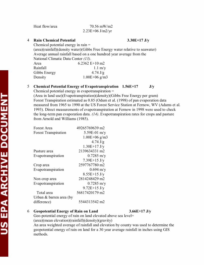
5 Chemical Potential Energy of Evapotranspiration 1.56E+17 J/y Chemical potential energy in evapotranspiration =

(Area in land use)(Evapotranspiration)(density)(Gibbs Free Energy per gram) Forest Transpiration estimated as 0.85 (Odum et al. (1998) of pan evaporation data

measured from 1965 to 1990 at the US Forest Service Station at Fernow, WV (Adams et al. 1993). Direct measurements of evapotranspiration at Fernow in 1998 were used to check the long-term pan evaporation data. (14). Evapotranspiration rates for crops and pasture from Arnold and Williams (1985).

Forest Area 49265769639 m2 Forest Transpiration 5.59E-01 m/y 1.00E+06 g/m3 4.74 J/g 1.30E+17 J/y Pasture area 2139634331 m2 Evapotranspiration 0.7285 m/y 7.39E+15 J/y Crop area 2597767780 m2 Evapotranspiration 0.694 m/y 8.55E+15 J/y Non crop area 2814248429 m2 Evapotranspiration 0.7285 m/y 9.72E+15 J/y Total area 56817420179 m2 Urban & barren area (by

difference) 5544313542 m2

6 Geopotential Energy of Rain on Land 3.66E+17 J/y Geo-potential energy of rain on land elevated above sea level= (area)(mean elevation)(rainfall)(density)(gravity) An area weighted average of rainfall and elevation by county was used to determine the geopotential energy of rain on land for a 30 year average rainfall in inches using GIS methods.

Table C1.1. Data used to determine the geopotential energy of rainfall.

County Area m2 Avg. elevation m.

30 y avg. rainfall in. geopot. energy

Hancock 228191120 322.427524 37.38536 6.85386E+14 Brooke 240176944 314.537809 39 7.34128E+14 Ohio 281945344 335.586703 39 9.19469E+14 Marshall 807178112 348.82437 41.29286 2.89704E+15 Preston 1686139648 630.98804 50.8542 1.34817E+16 Morgan 595436736 276.183843 37.02715 1.51725E+15 Mononga. 947073856 404.950628 43.57846 4.16448E+15 Wetzel 934991488 360.850872 45.24491 3.80371E+15 Mineral 853182720 397.950762 35.54701 3.0073E+15 Berkeley 833351552 199.736011 37.40184 1.55124E+15 Marion 806174464 376.575944 44.14345 3.33926E+15 Tyler 674734592 293.881773 43.70897 2.15963E+15 Hampshire 1669929728 377.768439 35.88709 5.64111E+15 Jefferson 548594112 160.223237 37.32662 8.17519E+14 Pleasants 348228768 273.18179 42.34601 1.00376E+15 Harrison 1078628224 366.759651 44.31864 4.3686E+15 Taylor 454673568 415.159562 45.41841 2.13624E+15 Doddridge 829267712 335.091023 45.02627 3.11764E+15 Wood 975464832 243.702585 40.0934 2.37491E+15 Ritchie 1174552960 297.039562 43.1418 3.75049E+15 Grant 1243197696 641.02717 38.34443 7.61415E+15 Barbour 887184064 521.134496 48.06692 5.53749E+15 Tucker 1090434304 857.48782 52.06758 1.2131E+16 Hardy 1513710208 537.310292 36.46919 7.39089E+15 Wirt 608199552 268.670655 42.90828 1.74707E+15 Lewis 1008180032 377.391402 46.69351 4.42679E+15 Randolph 2691785216 911.070648 53.8217 3.28891E+16 Upshur 918238400 560.858453 50.26036 6.44966E+15 Gilmer 878942080 318.033214 44.5842 3.10539E+15 Jackson 1220555904 252.196695 42.61932 3.26894E+15 Calhoun 725900992 307.80376 43.69557 2.43272E+15 Mason 1152245888 227.116475 41.11225 2.68082E+15 Pendleton 1807532672 794.104907 38.86252 1.38995E+16 Roane 1252050048 296.208663 43.66887 4.03547E+15 Table C1.1 continued.

County Area m2 Avg. elevation m.

30 y avg. rainfall in. geopot. energy

Braxton 1337042688 376.932653 47.07839 5.91199E+15 Pocahontas 2437553408 989.455485 49.93845 3.00115E+16 Webster 1439527296 753.490796 52.94361 1.43092E+16 Putnam 906781952 251.909579 41.98552 2.38974E+15

Clay 889922560 372.487511 46.3062 3.82477E+15 Kanawha 2357247232 325.598119 44.10259 8.43439E+15 Cabell 745557888 639.549 42.71017 5.07445E+15 Nicholas 1693563264 639.549502 49.14842 1.32644E+16 Wayne 1326469120 272.992341 43.54009 3.92862E+15 Lincoln 1136250368 290.620653 44.14746 3.63253E+15 Greenbrier 2651428096 808.361377 45.13994 2.41073E+16 Fayette 1730641664 612.812798 45.63472 1.20596E+16 Boone 1302429440 428.168433 46.35194 6.4408E+15 Logan 1179267712 435.418879 46.64979 5.96859E+15 Raleigh 1576129536 704.715715 43.79303 1.21203E+16 Mingo 1097541376 403.322368 45.97489 5.07104E+15 Summers 951547136 672.4003 38.51943 6.14102E+15 Wyoming 1299047680 596.885295 45.0688 8.70752E+15 Monroe 1225340928 708.407376 38.52779 8.3333E+15 Mercer 1088748160 768.072665 37.73166 7.8621E+15 McDowell 1384392576 599.940657 42.65404 8.82735E+15 Total 6.2723E+10 3.655E+17

7 Geopotential of runoff 6.02 E+16 J/y

Geopotential energy of runoff (physical energy of streams) = (area)(mean elevation – (base elevation when > sea level)(runoff)(density)(gravity)

The annual runoff is a 30 year average. The elevation was also an average based on known elevations in the selected area (15).

Watershed (Great Cacapon, WV) Area 1.75E+09 m2 Elevation 609.6 m (Potomac, Harper’s Ferry) Base elev. 73.2 m Runoff/yr 0.3175 m/y Density 1000 kg/m3 Gravity 9.81 m/s2 Energy 2.93E+15 J/y (Bemis, WV) Area 2.98E+08 m2 Elevation 1987 m (Cheat R., Morgantown) Base elev. 250.5 m Runoff/yr 1.069 m/y Density 1000 kg/m3

Gravity 9.81 m/s2 Energy 5.420E+15 J/y (Little, WV) Area 1.09E+07 m2 Elevation 1215 m (Ohio R., Parkersburg) Base elev. 171.3 m Runoff/yr 0.48006 m/y Density 1000 kg/m3 Gravity 9.81 m/s2 Energy 5.358E+13 J/y (Buckeye, WV) Area 1.40E+09 m2 Elevation 2303 m (Ohio R., Point Pleasants) Base elev. 156.7 m Runoff/yr 0.5715 m/y Density 1000 kg/m3 Gravity 9.81 m/s2 Energy 1.683E+16 J/y (Clay, WV) Area 2.57E+09 m2 Elevation 1821 m (Ohio R., Point Pleasants) Base elev. 156.7 m Runoff/yr 0.68072 m/y Density 1000 kg/m3 Gravity 9.81 m/s2 Energy 2.855E+16 J/y (Julian, WV) Area 8.24E+08 m2 Elevation 1667 m (Ohio R., Huntington) Base elev. 149.1 m Runoff/yr 0.52578 m/y Density 1000 kg/m3 Gravity 9.81 m/s2 Energy 6.45E+15 J/y

8 River Chemical Potential Absorbed 2.90E+14 J/y Received 9.06E+16 J/y

River chemical potential energy received = (volume flow)(density)(Gibbs free energy relative to seawater)

River chemical potential energy absorbed = (volume flow)(density) (Gibbs free energy solutes at river entry – Gibbs free energy solutes at river egress)

The Ohio and New Rivers begin and end outside state boundaries delivering part of the chemical potential energy that they carry to the state.

Total Dissolved solids concentration from the USGS data (16). Gibbs Free energy, G = RT/w ln(C2/C1) = [(8.3143 J/mol/deg)(288 K)/(18 g/mol)] * ln [(1E6 - S)ppm)/965000]

Ohio River* Vol. flow 2.948 E+10 m3/yr (Water Data - USGS) Density 1000000 g/m3 Solutes in (at Sewickley, PA) 211.96 ppm G. in 4.711 J/g Solutes. out (Point Pleasant ) 295.55 G. out 4.700 J/g absorbed 3.279E+14 J/y received 1.389E+17 J/y New River Vol. flow 4.466 E+09 m3/yr (Water Data - USGS) Density 1000000 g/m3 Solutes in (Glen Lyn) 84 ppm G. in 4.728 J/g Solutes out (Point Pleasant ) 295.5 G. out 4.700 J/g absorbed 1.257E+14 J/y received 2.112E+16 J/y *If the river flows along the border the state, the energy was distributed equally between the states on opposite sides of the river.

9 River Geopotential Absorbed 2.06E+16 J/y

Received 4.99E+16 J/y Geopotential energy received (relative to sea level) = (flow vol.)(density)(height at entry) (gravity).

Geopotential energy absorbed = (flow vol.)(density)(height entry - height egress)(gravity) Ohio and New Rivers are the only rivers that begin and end outside of the state Data on water flow and height of the gauge are from USGS Water Resources Data (17).

Ohio River* Vol. Flow 2948 E+10 m3/yr ( Water data - USGS) Density 1000 kg/m3 Height In 207.26 m (Height at Sewickley, PA) Height Out 155.45 m (Height at Point Pleasant) Gravity 9.81 m/s2 Absorbed 1.499E+16 J/y Received 5.994E+16 J/y New River Vol. Flow 4.466 E+9 m3/yr (Water Data - USGS) Density 1000 kg/m3 Height In 454.23 m (at Glen Lyn, VA) Height Out 155.45 m (at Point Pleasant) Gravity 9.81 m/s2 Absorbed 1.309E+16 J/y Received 1.99E+16 J/y *If the river borders the state half the calculated energy was used

10 Agricultural Products 1.759E+16 J/y (amount sold)(energy/unit) Production data is from the West Virginia Agricultural Statistics Service Tables 42,43, and 37 in (18). Energy per unit value used was found in the USDA Nutrient Data Laboratory (1).

Hay Mass 8.0382E+11 g/y Energy/unit 18901 J/g 1.519E+16 J/y Oats 132,249 bushels/yr 14514.96 g/bushels Mass 1,919,588,945 g/y Energy/unit 16280 J/g 3.125E+13 J/y Wheat 421,453 bushels/y 27215.54 g/bushel Mass 11,470,070,980 g/yr Energy/unit 14230 J/g 1.632E+14 J/y

Corn 3,651,139 bushels/y 25401.17 g/bushels Mass 92,743,202,433 g/yr Energy/unit 19736 J/g 1.830E+15 J/y Tobacco Mass 2737090 lbs/y 1,241,522,948 g/y Energy/unit 14651 J/g 1.819E+13 J/y Soybeans 482,228 bushels/y 27215.54 g/bushels Mass 13,124,095,423 g/y Energy/unit 17,410 J/g 2.285E+14 J/y Apples Mass 52,394,370,290 g/y Energy/unit (1) 2160 J/g 1.142E+14 J/y Peaches Mass 4,615,592,663 g/y Energy/unit (1) 1650 J/g 7.616E+12 J/y Wool Mass 80,796,141 g/y Energy/unit 20934 J/g 1.691E+12 J/y

11 Livestock 4.00E+15 J/y (annual production mass)(energy/mass) The amount sold is taken from the 1997 Census of Agriculture (18). Turkeys # sold 4468456 wt 7257.5 g/animal Energy /unit (1) 6690 J/g All classes, meat and skin 2.170E+14 J/y Cows # sold 863647 wt 3.5E+05 g/animal Energy /unit (1) 12180 J/g Choice carcass 3.7E+15 J/y Hog/Pig # sold 24884 wt 9.00E+04 g/animal

Energy /unit (1) 15730 J/g Fresh carcass 3.52E+13 J/y Sheep/lamb # sold 40709 wt 68038.9 g/animal Energy /unit (1) 7406 J/g Raw leg, shoulder, arm 2.051E+13 J/y Horses # sold 16787 wt 476271.99 g/animal Energy /unit (1) 5560 J/g 4.445E+13 J/y

12 Fish Production 7.22E+11 J/y (mass)(energy/mass) Based on the 1998 trout sales of stocked fish reported by the US Department of Agriculture, 1998 Census of Aquaculture (19).

Mass 369,000 lbs/y 453.59 g/lb Energy/mass 4311.58 J/g

13 Hydroelectricity 4.09E+15 J/y Energy Information Administration, Electricity Net Generation by Fuel in West Virginia, 1997 (20).

14 Net Timber Growth 2.10E+17 J/y

Based on forest growth from 1975 to 1989, from the last inventory done for West Virginia by the U.S. Forest Service (21) (DiGiovanni 1990).

Forest Growth 491,132,000 ft3 1.39E+13 cm3 green wt 1 g/cm3 Forest growth 1.39E+13 g/y

15 Timber Harvest 2.29E+16 J/y Based on the forest statistics for West Virginia (21) DiGiovanni (1990). Forest Harvest 462,542,000 board ft 84,098,545 ft3 2.38E+12 cm3 dry wt 0.5 g/cm3 Forest mass 1.19E+12 g/y

16 Groundwater Chemical Potential Energy 9.49E+14 J/y (vol.)(density)(Gibbs free energy) Based on the volume of ground water withdrawn in 1995 (22). G = RT/w ln(C2/C1) = [(8.3143 J/mol/deg)(288 K)/(18 g/mol)] * ln [(1E6 - S)ppm)/965000]

Volume used 2.02E+08 m3/y (US Geological Survey on water use for state) Density 1000000 g/m3 S 342 ppm Gibbs 4.69 J/g

C2 Notes for Table 5 – Annual Production and Use of Nonrenewable Resources in 1997.

17 Coal Production 4.64E+18 J/y Provided by the West Virginia Department of Energy (23). Unit conversions may be found at (24). Short tons/y 1.74E+08 g/short ton 9.07E+05 J/g 2.94E+04

18 Coal Used in the State 9.92E+17 J/y Provided by the West Virginia Department of Energy (23). Short tons/y 3.72E+07 g/short ton 9.07E+05 J/g 2.94E+04

19 Natural Gas Production 1.89E+17 J/y

Taken from the Energy Information Administration Natural Gas Summary Statistics for Natural Gas - West Virginia, (25). The annual flows of natural gas are not exactly balanced because gas is taken and removed from underground storage. The flows balance over a longer averaging period. Amount 1.72E+08 1000 ft3 J/1000 ft3 1.1E+09

20 Natural Gas Used in the State 1.75E+17 J/y Taken from the Energy Information Administration Natural Gas Summary Statistics for Natural Gas - West Virginia (25). Amount 1.59E+08 1000 ft3 J/1000 ft3 1.1E+09

21 Petroleum Production 9.2E+15 J/y From Utah's Department of Natural Resources - Energy Office (26)

22 Petroleum Used in the State 2.3E+17 J/y (Energy Information Administration) From the State Energy Data Report of West Virginia 1960-1999. (27)

23 Electricity Production (without hydroelectricity) 3.26E+17 J/y

Energy Information Administration (28). Amount 90418730400 kW-hr

24 Electricity Used in the State 9.45E+16 J/y Energy Information Administration. From the State Energy Data Report of West Virginia 1960-1999. (27) 2.62E+10 kW hr Mineral Production Taken from the 1997 and 1998 Mineral Industry Studies of West Virginia by the US Geological Survey and the West Virginia Geological and Economic Survey (29).

25 Clay 151000 tons 2.96E+20 sej/y Emergy/Mass 1961864407 sej/g (From Odum 1996)

26 Sand and gravel 1670000 tons 3.34E+21 sej/y Emergy/Mass 1.31E+09 sej/g (Calculated in this study)

27 Limestone 12000000 tons 1.18E+22 sej/y Emergy/Mass 980932203 sej/g (From Odum 1996)

28 Sandstone 856 tons 8.40E+17 sej/y Emergy/Mass 980932203 sej/g (From Odum 1996)

29 Soil Erosion Total 5.03E+15 J/y Agricultural lands 3.99E+15 J/y (farmed area)(erosion rate)(organic fraction)(energy) The farmed area was taken from the 1997 census of Agriculture (18). The organic fraction was taken from Odum (1996). Erosion rates for cropland and pasture from the USDA (30) and for forest from Patric et al. (1984).

Cultivated Crop Area 641899.62 acres Erosion rate 4.3 ton/acre/yr Erosion 27601685 ton/yr Org. fraction 0.03 907185 g/ton 22604.4 J/g Energy 1.69803E+15 J/y

Non-Cultivated Farmed area 695391.26 acres Erosion rate 0.8 ton/acre/yr Erosion 556313 ton/yr

Org. fraction 0.03 907184.74 g/ton 22604.4 J/g Energy 3.42239E+14 J/y Pastureland Area 528696.4 acres Erosion rate 6 ton/acre/yr Erosion 3172178 ton/yr Org. fraction 0.03 907184.74 g/ton 22604.4 J/g Energy 1.9515E+15 J/y Forested Land Area 12173404.9 acres

Erosion rate 0.139 ton/acre/yr Erosion 1692103 ton/yr

Organic fraction 0.03

907184.74 g/ton 22604.4 J/g Energy 1.04097E+15 J/y The erosion rate for the forested land was measured at Shavers Fork, WV.

C3. Notes for Table 6 - Imports to the West Virginia economy in 1997.

30 Coal 2.32E+17 J/y Provided by the West Virginia Department of Energy (23). Short tons/yr 8.70E+06 g/short ton 9.07E+05 J/g 2.94E+04

31 Petroleum 2.2E+17 J/y Value is the difference between the production and consumption within the state. Also estimated from the data in the 1997 Commodity Flow Survey (2).

32 Natural Gas (Received at state border) 2.0E+18 J/y Taken from the Energy Information Administration data on Natural Gas (5). Most natural gas received passes through the state and thus it is not considered as an

import. This value would not usually be shown in an emergy analysis, but it is given here to a give an idea of the emergy flows linking the nation.

Summary Statistics for Natural Gas - West Virginia, Amount 1.79E+09 1000 ft3

J/1000 ft3 1.1E+09

33 Iron Ore 4.41E+13 J/y Data from Weirton Steel. Iron ore to satisfy 1997 production. 3.00E+06 tons/yr 2.72E+12 g/yr 16.2 J/g

34 Bauxite imported (corrected number) 4.4E+13 J/y Assume the ratio of bauxite ore to primary aluminum production is 4:1, alumina to

production is 2:1(Century Aluminum, Ravenswood WV). Aluminum production 1.7E+05 m ton/yr bauxite 6.7E+05 m ton/yr 6.7E+11 g/yr 6.5E+01 J/g

35 Emergy of Services in Goods Imported 2.99E+22 sej/y Data on shipments from the 1997 Commodity flow Survey, US. Census Bureau (2). Units Total in bound shipments 3.33E+10 $/y Shipments of West Virginia origin 8.34E+09 $/y Dollar value of imported goods 2.50E+10 $/y Emergy to dollar ratio for the US in1997 1.20E+12 sej/$ Emergy in the services embodied in imported goods 2.99E+22 sej/y

36 Emergy of Materials in Imported Goods (without fuels) 9.48E+22 sej/y Data on material shipments into West Virginia by commodity class from the 1997 Commodity Flow

Survey (2), Additional State Data, Table 12. See Appendix B for the calculation of average transformities for the SCTG commodity classes. Appendix D gives details of the method of calculation used here.

Table C3.1 Emergy imported to West Virginia in material commodity flows. SCTG Code Commodity Class J or g y-1

Emergy per unit Units

Emergy sej y-1

1 Live animals and live fish. 9.42E+13 4.39E+05 sej/J 4.14E+192 Cereal grains. 1.10E+15 1.82E+05 sej/J 1.99E+203 Other agricultural product. 2.09E+15 2.33E+05 sej/J 4.88E+204 Animal feed and products of animal origin. 4.58E+15 1.22E+06 sej/J 5.58E+215 Meat, fish, seafood, and their preparations. 1.91E+15 3.27E+06 sej/J 6.24E+216 Milled grain products and preparations. 2.93E+15 1.82E+05 sej/J 5.33E+207 Other prepared foodstuffs and fats and oils. 1.80E+16 1.12E+06 sej/J 2.01E+228 Alcoholic beverages. 3.62E+14 5.89E+04 sej/J 2.13E+199 Tobacco products. 6.05E+14 6.50E+05 sej/J 3.93E+20

10 Monumental or building stone. 3.23E+09 9.81E+08 sej/g 3.17E+1811 Natural sands. 3.69E+11 1.96E+09 sej/g 7.23E+2012 Gravel and crushed stone. 6.46E+12 4.91E+08 sej/g 3.17E+2113 Nonmetallic minerals. 7.30E+11 1.96E+09 sej/g 1.43E+21

14 Metallic ores and concentrates. 3.04E+10 2.71E+09 sej/g 8.23E+1915 Coal 2.25E+17 3.92E+04 sej/J 8.84E+2117 Gasoline and aviation turbine fuel. 1.07E+17 6.47E+04 sej/J 6.93E+2118 Fuel oils. 7.04E+16 6.47E+04 sej/J 4.56E+2119 Coal and petroleum products. 5.22E+16 6.47E+04 sej/J 3.38E+2120 Basic chemicals. 2.06E+12 2.75E+09 sej/g 5.65E+2121 Pharmaceutical products. 3.55E+10 2.75E+09 sej/g 9.77E+1922 Fertilizers 1.94E+11 2.99E+09 sej/g 5.80E+2023 Chemical products and preparations. 1.89E+11 9.90E+09 sej/g 1.87E+2124 Plastics and rubber. 4.61E+11 2.71E+09 sej/g 1.25E+2125 Logs and other wood in the rough. 3.24E+15 1.96E+04 sej/J 6.35E+1926 Wood products. 5.67E+11 1.49E+09 sej/g 8.44E+2027 Pulp, newsprint, paper, and paperboard. 6.01E+15 1.40E+05 sej/J 8.40E+2028 Paper or paperboard articles. 3.18E+15 1.67E+05 sej/J 5.33E+2029 Printed products. 6.58E+10 4.95E+09 sej/g 3.26E+2030 Textiles, leather, and articles. 1.74E+15 7.18E+06 sej/J 1.25E+2231 Nonmetallic mineral products. 2.46E+12 3.09E+09 sej/g 7.60E+2132 Base metal in primary or semi-finished form 1.30E+12 5.91E+09 sej/g 7.70E+2133 Articles of base metal. 4.42E+11 5.91E+09 sej/g 2.61E+2134 Machinery 1.15E+11 7.76E+09 sej/g 8.89E+2035 Electronic and other electrical equipment 1.57E+11 7.76E+09 sej/g 1.22E+2136 Motorized and other vehicles. 6.82E+11 7.76E+09 sej/g 5.29E+2137 Transportation equipment. 3.83E+10 7.76E+09 sej/g 2.97E+2038 Precision instruments and apparatus. 4.61E+09 7.76E+09 sej/g 3.58E+1939 Furniture, mattresses, lamps, lighting 4.81E+10 2.89E+09 sej/g 1.39E+2040 Miscellaneous manufactured products. 2.66E+11 1.61E+09 sej/g 4.29E+2041 Waste and scrap. 6.24E+11 2.16E+09 sej/g 1.35E+2143 Mixed freight. 5.85E+11 6.32E+09 sej/g 3.70E+210 Commodity unknown. 8.01E+10 ? ?

Total sej/y 1.19E+23 Total without fuels sej/y 9.48E+22

37 Services

The emergy in imported and exported services was determined using a variation of the base-nonbase method from economic analysis. Data on employment and revenues by NAICS sector for West Virginia and for the United States as whole (31) were used to estimate services exported and imported from the state using a modification of the location quotient and assumption methods. The formulae in the text are evaluated using data from the tables below.

Table C3.2 Export and Import of Services Between West Virginia and the Nation Economic Sectors

Parameters Agricult.. Mining Utilities Construct. Manufact. Wholesale Retail trade Transport. Informat. US sector (Ni) 0.0249 0.0041 0.0057 0.0457 0.1362 0.0467 0.1128 0.0236 0.0247 State Sector (Si) 0.0337 0.0349 0.0113 0.0457 0.1062 0.0347 0.1314 0.0212 0.0173 (Si - Ni ) 0.0089 0.0308 0.0057 0.0000 -0.0300 -0.0120 0.0186 -0.0024 -0.0074 $/employee US 70034 341821 585899 151563 227502 700357 175889 108959 203255 $/emp. WV 19321 264699 420160 99198 251237 432277 156048 136256 149509

Location Quotient 1.36 8.50 2.00 1.00 0.78 0.74 1.16 0.90 0.70(Si) ÷ (Ni) 0.007 0.047 0.011 0.006 0.004 0.004 0.006 0.005 0.004(St) ÷ (Nt) 0.006 0.006 0.006 0.006 0.006 0.006 0.006 0.006 0.006Basic jobs (B) 6075.20 21113.14 3882.36 -4.04 -20546.35 -8239.19 12742.19 -1620.47 -5088.21Exp(+) or imp(-) $* 1.17E+08 5.59E+09 1.63E+09 -6.12E+05 -4.67E+09 -5.77E+09 1.99E+09 -1.77E+08 -1.03E+09Services in Sector none part part imports none Local (no) Local (no) Local (no) imports Assumption Base Base Base nonbase Base nonbase nonbase nonbase nonbase $ value of goods all goods 5.03E+09 1.38E+09 all goods Services exported# 0 5.61E+08 2.48E+08 0 *Export is determine by multiplying basic jobs by the $/employee in the West Virginia sector. Potential import is determined by multiplying the basic job deficit by the $ per employee in the U.S. sector. Basic sectors can export. # The export sectors summed here are only part service at this level of sector aggregation. Subtracting the dollar value of the goods exported in the sector from total estimated exports gives an estimate of the services exported. An alternative method (Table C3.2) considers higher resolution sector data where the export sectors evaluated are all service. Economic Sectors continued:

Finance& Insurance

RealEstate& Rental

Profession. Scientific Managem.

Administ. Support

Education Services

HealthCare Social Ser.

Arts& Entertain.

Accomo.& Food

US sector (Ni) 0.0471 0.0137 0.0432 0.0211 0.0593 0.0026 0.1094 0.0128 0.0762State Sector (Si) 0.0308 0.0085 0.0240 0.0069 0.0313 0.0012 0.1397 0.0096 0.0752 (Si - Ni ) -0.0162 -0.0053 -0.0192 -0.0142 -0.0280 -0.0014 0.0303 -0.0032 -0.0010$/employee US 376639 141515 111029 35328 40278 63659 65262 65956 37074$/employee WV 205448 114420 75120 30082 37138 45921 60844 49389 31694 Location Quot. 0.66 0.62 0.56 0.33 0.53 0.47 1.28 0.75 0.99(Si) ÷ (Ni) 0.004 0.003 0.003 0.002 0.003 0.003 0.007 0.004 0.005(St) ÷ (Nt) 0.006 0.006 0.006 0.006 0.006 0.006 0.006 0.006 0.006Basic jobs (B) -11113.89 -3599.22 -13175.53 -9750.06 -19172.28 -931.94 20767.66 -2205.81 -718.72Exp(+) imp(-) $* -4.19E+09 -5.09E+08 -1.46E+09 -3.44E+08 -7.72E+08 -5.93E+07 1.26E+09 -1.45E+08 -2.66E+07Services in Sector Imports Local (no) Imports Imports Imports Imports Local (no) Imports Imports Assumptions nonbase nonbase nonbase non base nonbase nonbase nonbase nonbase Base Sectors continued:

Other Ser. Auxillar. Governm. US sector (Ni) 0.0263 0.0064 0.1576State Sector (Si) 0.0264 0.0071 0.2028 (Si - Ni ) 0.0002 0.0007 0.0452$/employee US 81659 14231 141198$/employee WV 64655 1279 51394 Location Quot. 1.01 1.11 1.29(Si) ÷ (Ni) 0.006 0.006 0.007(St) ÷ (Nt) 0.006 0.006 0.006Basic jobs (B) 112.39 492.67 30980.10Exp(+) imp(-) $* 7.27E+06 6.30E+05 1.59E+09Services in Sector Local (no) Local (no) Local (no)Assumptions nonbase nonbase Base

Table C3.3 Alternative Method for Determining Exports: Detailed Analysis of the Mining and Utilities sectors

Drilling oil & gas wells

Support activities for oil & gas

Support activities for coal

Electric services

US sector (Ni) 0.0004 0.0009 0.0000 0.0020State Sector (Si) 0.0007 0.0014 0.0021 0.0032(Si - Ni ) 0.0003 0.0006 0.0021 0.0012$/employee US 138072 5451 22610483 465837$/employee WV 77043 77270 135639 398779 Location Quot. 1.7317 1.6791 52.6411 1.6347(Si) ÷ (Ni) 0.0096 0.0093 0.2910 0.0090(St) ÷ (Nt) 0.0055 0.0055 0.0055 0.0055Basic jobs (B) 214 398 1425 850Exp(+) imp(-) $* 1.65E+07 3.08E+07 1.93E+08 3.39E+08Service exported ($) 5.80E+08

Table C3.4 Determination of Imported and Exported Services Potential for Importing ($)

8.01E+09Multiply deficit employment times U.S. worker productivity in sectors assumed to be capable of importing services in Table C3.1 and sum over the sectors.

Fraction of potential ($) imported

6.17E+09

We assume that states with average per capita income can import the services deficit and that states below US avg. per capita income can import a fraction of the deficit equal to average per capita income of the state /average U.S. per capita income. In 1997 this fraction was $19628/$25412 or 0.77 for West Virginia. Multiply potential imports by 0.77 to estimate imported services.

Emergy in exported services sej/y

7.0E+20

Multiply the basic employment in the detailed service sectors above by West Virginia worker productivity and sum. Multiply this dollar amount by the emergy to dollar ratio of the U.S. in 1997 to estimate the emergy exported

Emergy in imported services sej/y 7.4E+21

Product the imported services times the emergy to dollar ratio of the U.S. in 1997.

Table C3.5 West Virginia employment by sector and the dollars generated per employee, 1997.

Sectors NAICS Number of Sales, Revenues, Dollars per Percent of total Employees Shipments Employee Employees 1000 $

Agriculture 23135 447000 19321.37454 0.033749876Mining 23927 6333463 264699.4191 0.034905264Utilities 7767 3263383 420160.036 0.01133068Construction 31312 3106093 99198.16684 0.045678674Manufacturing 72813 18293309 251236.8533 0.106221298Wholesale trade 23805 10290356 432277.0846 0.034727288Retail trade 90087 14057933 156048.4088 0.131421011Transportation 14526 1979257 136256.1614 0.021190867Information 11862 1773480 149509.3576 0.017304561Finance & Insurance 21144 4344000 205448.3541 0.030845359Real Estate & rental 5812 665011 114420.3372 0.008478681Professional Scientific 16462 1236618 75119.54805 0.024015148Management 4720 141988 30082.20339 0.006885646

Administrative support 21445 796429 37138.21404 0.031284465Education services 843 38711 45920.52195 0.001229788Health care & social services 95738 5825082 60843.99089 0.139664821Arts& entertainment 6571 324534 49388.82971 0.009585928Accommodation & food 51529 1633164 31694.07518 0.075171703Other services 18113 1171099 64655.1648 0.026423666Auxiliaries 4873 6235 1279.499282 0.007108846Government 139000 7143800 51394.2446 0.202776432

Table C3.6 US employment and productivity by Industry sector, 1997 Sectors NAICS Employees Sales, receipts or Dollars per Fraction of total shipments $1000s Employee Employees Agriculture 3085992 216125000 70034.20618 0.024887236Mining 509006 173988778 341820.6819 0.004104921Utilities 702703 411713327 585899.4867 0.005667006Construction 5664840 858581046 151563.1591 0.045684568Manufacturing 16888016 3842061405 227502.2362 0.136194793Wholesale trade 5796557 4059657778 700356.7425 0.04674681Retail trade 13991103 2460886012 175889.35 0.1128324Transportation 2920777 318245044 108959.0352 0.023554846Information 3066167 623213854 203255.0262 0.024727356Finance & Insurance 5835214 2197771283 376639.3628 0.047058563Real Estate & rental 1702420 240917556 141514.759 0.013729306Professional Scientific 5361210 595250649 111029.1611 0.043235919Management 2617527 92473059 35328.40693 0.021109262Administrative support 7347366 295936350 40277.88326 0.059253437Education services 321073 20439028 63658.50757 0.00258932Health care & social services 13561579 885054001 65261.86965 0.109368469Arts& entertainment 1587660 104715028 65955.57487 0.012803815Accommodation & food 9451226 350399194 37074.46992 0.076220189Other services 3256178 265897685 81659.44399 0.026259715Auxiliaries 792370 11275968 14230.68516 0.006390133Government 19540000 2759000000 141197.5435 0.157581936 Table C3.7 West Virginia detailed export sector employment and the dollars generated per employee.

Sectors NAICS Number of Sales, Revenues, Dollars per Percent of total Employees Shipments Employee WV Employees 1000 $

Mining Services 2944 312178 106038.7228 0.004294776Drilling oil&gas wells 506 38984 77043.47826 0.000738165Support activities 985 76111 77270.05076 0.001436941

for oil & gas Support activities for coal 1453 197083 135638.6786 0.00211967Electric services (electric power distribution)) 2190 873325 398778.5388 0.003194823 Table C3.8 U.S. employment in detailed export sectors and the dollars generated per employee, 1997. Sectors NAICS Employees Sales, receipts or Dollars per Fraction of total shipments $1000s Employee US Employees Mining Services 168806 19898686 117879.0209 0.00136135Drilling oil&gas wells 52858 7298223 138072.2502 0.000426278Support activities for oil & gas 106118 11501280 5450.997946 0.000855797Support activities for coal 4993 578449 22610483.28 4.02665E-05Electric services (electric power distribution)) 242347 112894143 465836.7671 0.001954427

38 Federal Government Personal Income Tax 2631000000 $/y Data Source: (33) Social Security Tax 2150000000 $/y State of West Virginia (1999) Business Taxes 2067026316 $/y State of West Virginia (1999) Total Tax (effective export) 6.85E+09 $/y Total Outlay to government and

individuals 1.04E+10 $/y From the U.S. Statistical Abstract for 1998 (33)

Net Gov. Funds spent in WV 3.56E+09 $/y (1.04E+10)-(6.85E9)

C4. Notes for Table 7 - Exports from the West Virginia Economy in 1997.

39 Coal 3.82E+18 J/y Provided by the West Virginia Department of Energy (23). Short tons/yr 1.43E+08 g/short ton 9.07E+05 J/g 2.94E+04

40 Natural Gas (Production Exports) 6.65E+15 J/y Calculated from the Energy Information Administration Natural Gas Summary Statistics for Natural Gas - West Virginia (25), Export is production – consumption. Amount 6.05E+06 1000 ft3 J/1000 ft3 1.1E+09

41 Natural Gas (Delivered at state border) 2.08E+18 J/y

Taken from the Energy Information Administration Natural Gas (5). See Note 32 on the natural gas received at the state border.

Summary Statistics for Natural Gas - West Virginia (25). Amount 1.89E+09 1000 ft3 J/1000 ft3 1.1E+09

42 Electricity 2.35E+17 J/y Energy Information Administration, (28). From the State Energy Data Report of West Virginia 1960-1999 (27). (Net generation)-(Consumption) 6.53E+10 kW h

43 Steel 2.00E+12 g/y From Greg Warren at Weirton Steel in Wheeling, West Virginia 2.20E+06 ton/y

44 Services embodied in exported goods. Data on shipments from the 1997 Commodity Flow Survey (2). Data on electricity from EIA (27). Electricity is not included in the CFS data. Units Total shipments to all destinations 3.56E+10 $/y Shipments to West Virginia destinations 8.34E+9 $/y Dollar value of exported goods (2) 2.72E+10 $/y Emergy to dollar ration for the US in 1997 1.20E+12 sej/$ Emergy exported in the services embodied in

goods including fuels. 3.27E+22 sej/y Dollars paid for electricity @ .05 $/KWh (27) 3.27E+09 $ Emergy in services in Electricity exported 3.92E+21 sej/y Total Emergy in services embodied in goods. 3.66E+22 sej/y Dollars paid for coal 3.92E+09 $ Emergy in services in coal exported 4.70E+21 sej/y

45 Material in exported goods Data on material shipments from West Virginia to all states by commodity is from The U.S. Census Bureau’s 1997 Commodity Flow Survey (2), Additional State Data, Table 12. In cases below shipment weight from the commodity flow survey was converted to energy. See Appendix B for the calculation of average emergy per unit for the commodity classes and a table giving the mass to energy conversions for the commodity class.

Table C4.1 Emergy in the materials exported from West Virginia SCTG Code Commodity Class

J or g

Emergy per unit Units

Emergy sej y-1

1 Live animals and live fish. 0 4.393E+05 sej/J 02 Cereal grains. 0 1.818E+05 sej/J 03 Other agricultural product. 0 2.334E+05 sej/J 04 Animal feed and products of animal origin. 4.034E+14 1.217E+06 sej/J 4.471E+205 Meat, fish, seafood, and their preparations. 1.720E+15 3.270E+06 sej/J 5.624E+216 Milled grain products and preparations. 2.857E+13 1.818E+05 sej/J 5.195E+18

7 Other prepared foodstuffs and fats and oils. 0 1.120E+06 sej/J 08 Alcoholic beverages. 0 5.886E+04 sej/J 0

Table C4.1 continued SCTG Code Commodity Class

J or g

Emergy per unit Units

Emergy sej y-1

9 Tobacco products. 1.595E+14 6.500E+05 sej/J 1.037E+2010 Monumental or building stone. 0 9.810E+08 sej/g 011 Natural sands. 4.046E+11 1.962E+09 sej/g 3.969E+2012 Gravel and crushed stone. 1.660E+11 4.905E+08 sej/g 8.143E+1913 Nonmetallic minerals. 0 1.962E+09 sej/g 014 Metallic ores and concentrates. 0 2.711E+09 sej/g 015 Coal 3.82E+18 3.924E+04 sej/J 1.500E+2317 Gasoline and aviation turbine fuel. 0 6.475E+04 sej/J 018 Fuel oils. 4.021E+14 6.475E+04 sej/J 2.604E+1919 Coal and petroleum products. 1.26E+17 6.475E+04 sej/J 8.170E+2120 Basic chemicals. 3.860E+12 2.750E+09 sej/g 1.061E+2221 Pharmaceutical products. 0 2.750E+09 sej/g 022 Fertilizers 0 2.993E+09 sej/g 023 Chemical products and preparations. 5.951E+11 9.902E+09 sej/g 5.893E+2124 Plastics and rubber. 8.428E+11 2.709E+09 sej/g 2.283E+2125 Logs and other wood in the rough. 2.9667E+16 1.962E+04 sej/J 5.821E+2026 Wood products. 2.562E+12 1.490E+09 sej/g 3.816E+2127 Pulp, newsprint, paper, and paperboard. 1.398E+05 sej/J 028 Paper or paperboard articles. 5.752E+14 1.674E+05 sej/J 9.631E+1929 Printed products. 0 4.951E+09 sej/g 030 Textiles, leather, and articles. 0 7.177E+06 sej/J 031 Nonmetallic mineral products. 1.224E+12 3.094E+09 sej/g 3.787E+21

32 Base metal in primary or semi-finished form 4.802E+12 5.906E+09 sej/g 2.836E+22

33 Articles of base metal. 3.502E+11 5.906E+09 sej/g 2.068E+2134 Machinery 1.261E+11 7.755E+09 sej/g 9.779E+2035 Electronic and other electrical equipment 8.375E+10 7.755E+09 sej/g 6.495E+2036 Motorized and other vehicles. 4.107E+11 7.755E+09 sej/g 3.185E+2137 Transportation equipment. 0 7.755E+09 sej/g 038 Precision instruments and apparatus. 0 7.755E+09 sej/g 039 Furniture, mattresses, lamps, lighting 2.994E+10 2.890E+09 sej/g 8.652E+1940 Miscellaneous manufactured products. 9126E+10 1.613E+09 sej/g 1.472E+2041 Waste and scrap. 0 2.161E+09 sej/g 043 Mixed freight. 1.007E+11 6.316E+09 sej/g 2.064E+200 Commodity unknown. 0 ? ? Natural Gas (joules) 4.80E+04 sej/J 3.19E+20 Total 2.279E+23 Total without fuels (15,17,18, natural gas) 7.76E+22 Exported fuels 1.503E+23

46 Services See calculations at Note 37 above.

Dollar value of services exported 5.796E+08 $/y

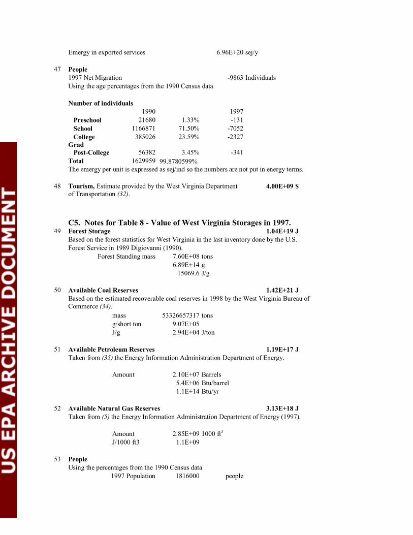
Emergy in exported services 6.96E+20 sej/y

47 People 1997 Net Migration -9863 Individuals Using the age percentages from the 1990 Census data Number of individuals 1990 1997 Preschool 21680 1.33% -131 School 1166871 71.50% -7052 College Grad

385026 23.59% -2327

Post-College 56382 3.45% -341 Total 1629959 99.8780599% The emergy per unit is expressed as sej/ind so the numbers are not put in energy terms.

48 4.00E+09 $ Tourism, Estimate provided by the West Virginia Department of Transportation (32).

C5. Notes for Table 8 - Value of West Virginia Storages in 1997. 49 Forest Storage 1.04E+19 J Based on the forest statistics for West Virginia in the last inventory done by the U.S. Forest Service in 1989 Digiovanni (1990). Forest Standing mass 7.60E+08 tons 6.89E+14 g 15069.6 J/g

50 Available Coal Reserves 1.42E+21 J

Based on the estimated recoverable coal reserves in 1998 by the West Virginia Bureau of Commerce (34).

mass 53326657317 tons g/short ton 9.07E+05 J/g 2.94E+04 J/ton

51 Available Petroleum Reserves 1.19E+17 J

Taken from (35) the Energy Information Administration Department of Energy.

Amount 2.10E+07 Barrels 5.4E+06 Btu/barrel 1.1E+14 Btu/yr

52 Available Natural Gas Reserves 3.13E+18 J

Taken from (5) the Energy Information Administration Department of Energy (1997).

Amount 2.85E+09 1000 ft3 J/1000 ft3 1.1E+09

53 People Using the percentages from the 1990 Census data 1997 Population 1816000 people

Number of individuals 1990 Fraction 1990 1997 Preschool 21680 0.0121 21952 School 1166871 0.6506 1181525 College Grad 379048 0.2113 383808 Post-College 50403 0.0281 51036 Elderly (65+) 157540 0.0878 159518 Public Status* 17935 0.0100 18160 Legacy# 792 792 *Public Status is estimated as one per cent of total population. #All individuals listed in the index to West Virginia: A History by O.K. Rice are counted as part of West Virginia’s legacy.

A few of those legacy individuals are: Henry Davis - West Virginian senator and democratic candidate for the Vice Presidency of the United States in 1904 (lost to Roosevelt and Fairbanks) Belle Boyd - confederate spy born in Martinsburg, WV John Brown - known for his actions at Harper's Ferry Pearl S. Buck - author who won the Nobel prize for literature in 1938, born in Hillsboro Alexander Campbell, religious leader and educator. Bethany College and the Disciples of Christ. Cornstalk - Shawnee Indian chief John Davis - constitutional lawyer who argued 140 cases in the Supreme Court, most at the time also the unsuccessful democratic candidate for the US Presidency in 1924 (lost to Coolidge), born in Clarksburg. Thomas J. “Stonewall” Jackson - confederate general, and exemplary leader. John Kenna - West Virginian representative and senator, born in St. Albans. Walter Reuther - president of the United Automobile Workers, born in Wheeling. Francis Pierpont - governor of the "Restored Government of Virginia" during the Civil War born in Morgantown Mary Harris "Mother" Jones - leader of strikers in the coal camps who fought for fair labor laws

C6. Notes for Table 9– Summary Flows for West Virginia in 1997

54 Renewable emergy sources received (Table 4) are the chemical potential energy in rain, the energy of the earth cycle, and the chemical potential energy in rivers. Renewable emergy sources absorbed by (used in) the system are the chemical potential energy of rain evapo-transpired, the geopotential of runoff doing work on the land, and the chemical potential and geopotential energy of the rivers used as the river flows through the state.

55 Nonrenewable sources (Table 5) include fuels and minerals coal, natural gas, petroleum, clay, sand and gravel, limestone and soil erosion where it exceeds soil building, i.e., in agricultural areas.

56 Dispersed Rural Source (Table 5) is the soil erosion in agricultural areas. This category includes any renewable resource that is being used more rapidly then it is being replaced.

57 Mineral Production (Table 5) is the emergy in the mined tonnage of coal, natural gas, petroleum, clay, limestone, sandstone, sand and gravel.

58 Fuels exported without use are the quantities of coal and natural gas exported without first being used in a production process in the state. (coal production + import – use = 1522 E+20 sej/y) compared to the commodity flow survey number for coal (1497 E+20 sej/y). Use commodity flow survey number and add 3 E+20 sej/y natural gas exports.

59 Imported minerals and fuels are coal, petroleum, iron ore and bauxite (Table 6).

60 Minerals used (includes fuels): Add mineral production and mineral imports and subtract fuels exported without use.

61 In state minerals used: Subtract minerals exported without use from mineral production.

62 The material imported in goods was determined from the 1997 Commodity Flow Survey by summing the tonnage by commodity class from states with significant exports to West Virginia. (see note 36).

63 Dollars paid for imports is the sum of the dollar value of imported goods including fuels and minerals and all other goods and services.

64 The services in imported minerals including fuels are determined below.

Table C6.1 Services in Imported Minerals

Amount $/amount $ Iron Ore (T) 3.0E+06 28.9 1.73E+08 Bauxite (T) 6.7E+05 27 1.8E+07 Coal (sT) 8.704E+06 26.64 2.32E+08 Petroleum (Btu) 2.09E+14 Petroleum (Barrels) 3.89E+07 Petroleum (Gal) 1.63E+09 0.799 1.31E+09

Total 1.73E+09

The prices of these items can be found in the data sources given at (36)

65 Dollars paid for goods without fuels and minerals is the total dollar value of goods imported from the CFS ($2.5E+10) minus the dollar value in fuels and minerals calculated above.

66 Dollars paid for imported services as determined using the base-nonbase method (Table C3.3).

67 Federal transfer payments are the total outlay of funds by the Federal government (note 38).

68 Imported Services Total is the sum of the emergy in services associated with imported goods, fuels, and minerals, and pure services.

69 Imported Services in fuels and minerals is the emergy equivalent of the human service represented by the money paid for fuels and minerals. Dollars are convert to emergy using the 1997 emergy/$ ratio for the US.

70 Imported Services in Goods is the emergy equivalent of the money paid for goods minus that paid for fuels and minerals. (use 1.2E+12 sej/$).

71 Imported Service is the emergy equivalent of the money paid for services (note 37).

72 Emergy purchased by Federal dollars spent in the state. Use West Virginia emergy/$ ratio.

73 Exported Products is the emergy in the goods exported including electricity (Table 7).

74 Dollars Received for Exports is the sum of the payments for all exported goods and services

75 Dollars Received for Exported Goods other than fuels, is the dollar value of the exported goods ($2.72E+10) less fuels.

76 Dollars Received for fuels and electricity are determined in Table C6.2.

Table C6.2 Services in Exported Fuels and Electricity 1997 prices

Amount $/amount $

Coal (Short T) 1.43E+08 26.64 3.8E+09

Natural Gas (tcf) 6.09E+06 3.00 1.8E+07

Total fuels 3.92E+09

Electricity (kWh) 6.53E+10 0.05 $/kWh 3.27E+09

77 Dollars Paid for Services as determined by the base-non-base method given in (Note 37).

78 Dollars spent by tourists in West Virginia from West Virginia Dept. Transportation (32).

79 Federal Taxes Paid is the sum of personal income, social security, and business taxes (Note 38).

80 Total Exported Services is the sum of the emergy equivalents in human service in fuels, goods and services exported.

81 Exported Services in Fuels is the emergy equivalent of the human service in the dollars paid for fuels exported. Service is determined using the US emergy/$ ratio.

82 Exported Services in Goods is the emergy equivalent of the services embodied in all value added exported goods (goods and electricity minus fuels exported without use).

83 Exported service is the emergy equivalent of the dollar value of exported services (Note 37).

84 Emergy Purchased by Tourists is the emergy purchased when tourists $ are spent in West Virginia, i.e., at West Virginia’s emergy to dollar ratio.

85 Emergy Purchases Forgone is the emergy equivalent of taxes paid to the Federal government. This number was determined using the West Virginia Emergy/$ ratio.

86 Gross State Product of the State of West Virginia in 1997.

C7. Notes for Table 10: Calculation of Emergy Indices.

87 Renewable Emergy received (note 54).

88 Renewable Emergy Absorbed (note 54).

89 In-State Nonrenewable Use is the sum of dispersed rural sources (N0) and in-state mineral production (N1).

90 Imported Emergy is the sum of imported minerals (F), goods (G), and services (PI).

91 Total Emergy Inflow is the sum of renewable emergy received (Rr), and the emergy imported in the previous note.

92 The total emergy used in the state (U) is the sum of the renewable emergy absorbed (Ra), the emergy used form dispersed rural sources (N0), fuels and minerals used (F1), and the goods (G) and services (PI) imported.

93 Total exported emergy is the sum of the emergy in the materials of exported goods (B), the emergy of services associated with goods and with pure service (PE) and the emergy of fuels and minerals exported without use (N2).

94 The emergy used from home sources is the sum of emergy from dispersed rural sources, in-state minerals and fuels used (F2), and renewable emergy absorbed divided by total use (U).

95 Import minus export is the difference between imported emergy (note 90) and exported emergy (note 93).

96 Ratio of exports to imports is the quotient of the expression in note 93 divided by the expression in note 91.

97 Fraction of use that is locally renewable is the ration of renewable emergy absorbed to total use.

98 Fraction of use that is purchased is the ratio of imported emergy (note 90) to total use (note 92).

99 Fraction of use in imported service is PI divided by U.

100 Fraction of use that is free is the sum of the renewable emergy absorbed and emergy from dispersed rural sources divided by total use.

101 Ratio of purchased to free is the quotient of the sum of imported fuels and minerals (F1), imported goods (G) and imported services (PI) divided by the sum of the renewable emergy received (Rr) and the emergy from dispersed rural sources (N0).

102 Environmental loading ratio is the quotient of the sum of the emergy from dispersed rural sources (N0), imported fuels and minerals (F1), imported goods (G) and imported services (PI) divided by the renewable emergy received (Rr).

103 Investment Ratio. There are several possible investment ratios (Odum 1996). This one compares imported emergy (note 90) to the emergy supplied form within the state. The emergy from within the state is the sum of the renewable emergy received (Rr), the emergy from dispersed rural sources (N0), and the emergy from in-state fuels and minerals (F2).

104 Emergy use per unit area (Empower density) is the total emergy use (U) divided by the area.

105 Use per person id the total emergy U divided by the population.

106 Renewable carrying capacity at the present standard of living is found by dividing the renewable emergy received by total use and then multiplying this fraction time the present population.

107 Developed carrying capacity at the present standard of living is approximately eight times the renewable carrying capacity.

108 West Virginia State Economic product (note 86).

109 Ratio of West Virginia emergy use to GSP. Divide U by X.

110 Ratio of U.S. Emergy use to GNP. See Appendix B3.2.

111 Ratio of emergy in electricity use to total use (El/U). See Table 5 for electricity use.

112 Ratio of electricity production to total use (Elp/U). ). See Table 5 for electricity production.

113 Fuel use per person is the sum of coal, natural gas, and petroleum used in the state (Table 5, 620E+20 sej/y) divided by population.

114 Population of the State in 1997

115 Area of the State

Appendix D.

Calculating Imports and Exports of Materials and Services

D1. Creating Export/Import Spreadsheets for Materials The method used to determine the emergy exported from and imported to West Virginia was further developed in this study to take advantage of the extensive data on this subject provided by the U.S. Census Bureau’s Commodity Flow Survey (2), which is performed every five years. This innovation resulted in a marked improvement in the accuracy with which imports and to a lesser extent exports to a state’s economy can be determined. Even though the CFS provides all the information needed to document exports and imports it is not tabulated in the form that we need and some of the information is hidden rather deeply in the data base. To make our method transparent and reproducible, we have described in detail the characteristics of the database, data sources and methods that we used to determine the emergy imported and exported from West Virginia. These methods should be applicable to the determination of imports and exports for any other state. To facilitate following the method described below the appropriate tables from the CFS should be accessed when needed. If the data tables or presentation of information change in the future these instructions will have to be altered. Export Calculations Determining material and energy flows for exports is straightforward with few extrapolations or assumptions needed, because the data are relatively complete as provided in the CFS. Data on dollar value and tonnage of export shipments between states by commodity class comes from the Commodity Flow Survey (CFS), Table 12 (Additional State Data). This data is also summarized in Tables 5, 7, and 8 in the CFS. The CFS uses several data codes when a numeric measurement is not given and these codes were handled in a consistent manner. For example, most states have an S or a D in one or more data fields for some commodity shipments. These letters indicate variable data (S) or a single source of information (D) that would risk disclosure. In the export calculation method, no estimate of exports was made for commodity classes with and S or D in both the $ value and tonnage columns for instate shipments. When this occurs there is often an S or a D in the “all destinations” category, as well. In this case there are too many unknowns to make an estimate. Materials moving in these classes were assumed to remain within the state or to constitute a negligible fraction of exports. Commodities with a dollar value but no information on tonnage were retained in the data because the tonnage could be reasonably estimated using the price per ton obtained from the dollar value and tonnage of the commodity going to all destinations. Before transferring data from Table 12 to an interim spreadsheet, all dashes (indicating no data) were replaced with zeroes. If there was evidence that some flows were not actually zero, remain uncounted, or are different from the estimates provided, additional information was added when the emergy exported in each commodity class was determined. For example, coal exports were determined using Energy Information Administration (EIA) Data. The Commodity Flow Survey provides a summary table (Table 7) of shipments to all states from the state of origin. Note that the top row in this table gives the total dollar value and tonnage of shipments from the state followed by a set of rows for dollar value and tonnage shipments to each state to which the state of origin is shipping. This includes a row for the state of origin itself, which will be referred to as instate shipments from now on. An export table (see Table D 1.2) with 11 columns was made to use in determining the tonnage exported in various commodity classes. The commodity classes for SCTG, SIC, and NAICS industry classification codes and the approximate conversions used in this paper are shown in Table D1.1. The column headings for the export table are as follows (1) SCTG code, (2) Description of the class, (3) All Destinations Value($ mil), (4) All Destinations Tons(000), (5) $/Ton, (6) Instate Shipments ($ mil), (7) Instate Shipments Tons(000), (8) Known (directly measured) exports Tons(000), (9) Instate Tons (000) estimated using $/T, (10) Estimated exports tons (000), (11) Final Exports (estimated exports are adjusted to sum to the total missing tonnage). . Table D 1.2 omits column 2, the verbal description, because of space considerations.

Table D1.1. Approximate conversion between SCTG , SIC and NAICS industry classification codes developed for this study. These conversions are only approximate and better information might be developed of used if available. Class Combined Code SCTG code SIC code NAICS Code agricultural products, grain A 2,3 1 111 livestock, seafood, animal products B 1,4 2,9 112 logs, rough wood C 25 8 113 metallic ores D 14 10 2122 coal E 15 12 2121 non-metallic minerals, gravel, stone, sand

F 11,12,13 14 2123

prepared food products, alcohol, tobacco G 5,6,7,8,9 20,21 311,312 textiles, leather, apparel H 30 22,23,31 313 lumber wood product I 26 24 321 furniture, fixtures J 39 25 337 paper products K 27,28 26 322 printed products L 29 27 323 chemicals M 20,21,22,23 28 325 refined petroleum products N 17,18,19 29 324 plastics and rubber O 24 30 326 building materials, non-metallic P 10,31 32 327,331 primary metal products, semi-finished Q 32 33 331 fabricated metal products. Cans etc. R 33 34 332 machinery (not electrical) S 34 35 333 electrical equipment , precision instruments

T 35.38 36,38 334,335

transportation equipment U 36,37 37 336 miscellaneous manufactured goods V 40 39 339 scrap and waste W 41 49 (?) 562 (?) unknown, mixed or special classes Y 43 92,98,99 99999 The steps in estimating exports from a state, e.g., West Virginia, using the data in the spreadsheet columns described above are as follows: First, copy the Commodity Class code and description from the Commodity Flow Survey Table 12 (Additional Data) for the state, for which exports are to be calculated Columns (1 and 2). Remember in following the instructions below that column numbers refer to the 11 column headings recommended above. The 10 columns shown in Table D 1.2, which is missing column 2, have been numbered to match the verbal description. 1. Copy the $ value and tons moving from the state to all destinations for all commodities, Columns (3) and (4). 2. Calculate the $ per ton. Column (5) 3. Copy data ($ and Tonnage) for shipments of all commodities with final destination in the state of origin, e.g., from WV to WV, Columns (6) and (7). 4 Calculate known exports by subtracting instate shipments (column 7) from the shipments moving to all destinations (column 4) for all commodities for which tonnage has been measured, directly, Column (8).

5. Sum the tonnage of directly measured export shipments (Column 8) and subtract from the total tonnage moving to all destinations. The total tonnage is given at the top of the All Destinations column in Table D 1.2 and in CFS Table 12. 6. Calculate the tonnage of instate shipments for any commodity for which a $ value of instate shipments is given in column 6 by dividing by the $ per ton (column 5). Record in Column 9 the estimated instate shipments. 7 Estimate the tonnage exported in these commodity classes by subtracting the instate tonnage estimates (column 9) from tonnage moving to all destinations (column 4). Record these estimates in Column 10. 8. Sum the estimated export shipments (column 9) and divide into the difference between directly measured exports and total exports. If this ration equals 1 combine directly measured and estimated exports in their respective commodity classes into a single column (11) and you are done. If greater or less than 1 multiply each estimated commodity by this ratio to adjust the flows so that directly measured and estimated exports will sum to the known tonnage of total exports shipped to all destinations. Record these numbers in Column (11), Final Adjusted Exports, and fill in column with the directly measured values from Column (8).

Table D1.2. Calculation of West Virginia Exports from the state to state commodity shipments found in the Commodity Flow Survey as Additional Data in Table 12.

SCTG Code

All DestinationsValue($ mil)

All DestinationsTons(000) $/ton

Instate Value (mil $)

Instate Tons (000)

Directly Measured Exports

Estimate Instate Tons(000)

Estimate State Exports

Final AdjustedExports

Col. 1 Column 3 Column 4 Col. 5 Col. 6 Col. 7 Col.8 Col.9 Col. 10 Col. 11 Total 35570 233760 8336 66249 167511 167511

1 - - 0 - - 0 02 - - 0 - - 0 03 S S 356 S S S S 04 129 467 276 87 438 29 295 609 259 2351 50 21 238 2386 29 14 2071 20 11 3 37 223 S 843 S S S S 08 365 351 1040 365 351 0 09 440 19 23158 177 7 12 12

10 S S 94 S S S S 0Table D1.2 continued

SCTG Code

All DestinationsValue($ mil)

All DestinationsTons(000) $/ton

Instate Value (mil $)

Instate Tons (000)

Directly Measured Exports

Estimate Instate Tons(000)

Estimate State Exports

Final AdjustedExports

11 32 793 40 4 347 446 44612 53 5667 9 51 5484 183 18313 S S 29 S S S S 014 S S 689 S S S S 015 4943 187835 26 1107 44488 143347 14334717 393 S 272 S S S S 018 227 964 235 224 954 10 1019 532 3335 160 78 163 3172 317220 3918 5152 760 425 897 4255 425521 1996 S 32716 S S S S 0

22 S S 216 S S S S 023 1512 946 1598 518 290 656 65624 2582 1316 1962 485 387 929 92925 370 5627 66 132 S S 2007 3620 340626 900 3869 233 216 1045 2824 282427 69 108 639 S S S S 028 123 87 1414 58 S S 41 46 4329 483 S 2499 S S S S 030 S S 9097 S S S S 031 937 5007 187 263 3658 1349 134932 4158 6306 659 449 S S 681 5625 529433 860 851 1011 525 465 386 38634 2109 187 11278 483 48 139 13935 1326 120 11050 242 S S 22 98 9236 2900 519 5588 212 S S 38 481 45337 320 S 10622 S S S S 038 234 2 117000 S - S S 039 159 45 3533 57 12 33 3340 692 134 5164 140 S S 27 107 10141 S S 148 S S S S 043 794 425 1868 605 314 111 111

-- 99 38 2605 S S S S 0

Class Totals 158122 9977 167511Difference (Total - Class Total from Column 7 in this Table. 9389 Fraction (Difference/Class Total (Column 7/Column 9 this table) 0.941

____________________________________________________________________________________ Transferring Export Data to the Emergy Evaluation Spreadsheet Columns 1, 2 and 11 beginning with SCTG code 1, can now be transferred to the emergy export evaluation section. Do not include commodities with zero flow. These are only shown in Table D 1.2 as placeholders to present a complete listing of all commodity categories. Import Calculations

Table 12 from the CFS web site, “Additional State Data”, used in the export calculation, has information on the exports by commodity class going from all the other states to the state of destination (West Virginia). Data from the other 49 states that might be exporting to the study state were combined to determine imports. Inbound shipments by state of origin to the state of destination are summarized in Table 8 of the CFS, but commodity classes are not shown. For states without a U.S. Customs port, state to state commodity shipments will capture almost everything entering the state. When one or more U.S. customs ports are located in a state the foreign imports entering the state need to be added, regardless of whether they are immediately exported to another state. We assume that these imports bring some value to the state by simply passing through.

The inbound tonnage shipped in each commodity category was used to calculate the emergy imported in goods. The five steps used to estimate imported emergy to a state are as follows: (1) a quick tally of the total tonnage coming into the study state from other states was obtained by consulting Table 8 in the CFS report. The states that had a number entered in the percent of total inbound shipments column were identified. The total percentage of imports directly measured was determined by summing the percentages. The total percent of tonnage from the states used to estimate imports should be at least 95% of the tonnage of total inbound shipments. (2) Once the subset of states exporting to the study state was identified, missing values for the tonnage for specific commodities coming from each state were estimated. (3) If a dollar value of the inbound commodity shipments was known and tonnage was not listed, the tonnage was estimated based on the cost per ton as described above and shown in Table D 1.2. A large fraction of total inbound shipments from some states had missing values for both dollar value and tonnage (an S or D entered into the field). In this case, the missing data would have resulted in large errors in the estimate of total imports and thus the development of a method to handle this situation was warranted. The tonnage fields for inbound shipments from a state of origin to West Virginia containing and S or a D were handled by assuming that a state’s exports to any other state would on average follow its overall export profile, i.e., the fraction of total shipments accounted for by each commodity. Missing tonnage data was distributed among commodity classes by adjusting the overall export profile. The missing tonnage data is equal to total shipments to West Virginia minus commodities with numeric entries for tonnage. This tonnage was distributed among the commodity classes with inbound shipments by adjusting the state’s overall export profile so that the unknown inbound shipments made up 100% of the missing inbound tonnage. (4) The inbound tonnage in each commodity class for a state was transferred as a single column to a second worksheet with data from all of the identified import states. (5) Then each commodity class was summed across the rows for all states to create the column of data with imported tonnages in each commodity class for the emergy table.

1. The following steps describe the estimation of the unknown tonnage (S and D) as illustrated for Alabama’s shipments to West Virginia shown in Table D 1.3. For all of the states importing to the study state, copy the total tonnage in each commodity class exported to all destinations and the tonnage exported to the state you are evaluating (columns 2 and 3 in Table D 1.3), onto a spreadsheet..

2. Calculate the price per ton for all inbound shipments by commodity class from any state exporting to the study state according to the instructions given above for exports.

3. Replace all dashes with a zero. Although Table D 1.3 only presents one state, the same procedure will be used for all states sending a significant quantity of imports to the study state.

4. Next, missing tonnage values are estimated for any commodity class that reported a dollar value of exports to the state but no tonnage. In some cases calculating the price per ton for the state of origin is not possible, but there is still a dollar value for exports. Prices per ton can be quite variable but find an adjacent state (or use a better estimation method) and substitute this price in the spreadsheet making a note on its origin. Fill in all tonnage movements possible using this method. Combine the tonnages estimated on the basis of average price with the tonnages that were directly measured. Sum this column and subtract from the total tonnage exported to the study state to get the tonnage that will be distributed using the export profile (see the number in italics at the top of column 4 in Table D 1.3). For example, the total export from Alabama to West Virginia is 318 thousand tons but the sum of all commodities determined directly and estimated based on dollar value only adds up to 27 thousand tons, the difference is then 291 thousand tons.

5. Create a fourth column for the export profile, which will be used to distribute the missing tonnage across the remaining commodities that had either an S or D in both the dollar value and tonnage fields. The export profile is the fraction of the total tonnage accounted for by each commodity as determined from the shipments to all destinations. Calculate the profile by dividing the tonnage for each commodity exported by the total tonnage exported for that state. Only those

commodities that have an S or D in both dollar value and tonnage fields are recorded in column 4. Sum the fractions to determine the fraction of total tons accounted for by the commodities with missing data.

6. The next step is to adjust these fractions to represent the expected fractions of the missing tonnage imported to the state in each commodity class with missing data. Create a fifth column, the adjusted fraction of missing tonnage imported in each class, where each fraction of the tons in the export profile (individual values in column 4) will be divided by the fraction of the total tons that is missing (the sum of all fractions in column four). The sum of all values in column 5 should equal one, or 100%.

7. In the last column (column 6), copy over the reported and estimated data for tonnage for any commodity where it is available from column 3. For all of the missing commodities (those with and S or D in both the $ value and tonnage fields), multiply the total missing tonnage (at the top of Column 4) by the corresponding percentage (in Column 5) for each commodity class known to have a flow but for which tonnage is unknown, and transfer this number to the appropriate field in column 6. For example, if data is missing for textiles, multiply 291 thousand tons by the fraction of textiles or 0.0172, to get 5 thousand tons textiles imported. Sum this column to make sure it adds up to the total tonnage.

8. Transfer this tonnage data for each commodity to an import table creating a column for each state.

9. Sum across the states (rows) for each commodity to find the total tonnage imported in each commodity class and transfer this to the import section of the emergy evaluation.

Custom’s Imports If the state has a Customs’ port, locate the appropriate data on the USITC data web site (37). The Customs’ site requires a password, but registration is free. To get the correct data report, a series of dialogue boxes must be completed. The choices that should be made are as follows: q Dialogue 1 – U.S. General Imports; NAICS code; current US Trade q Dialogue 2 – Customs value; 1997; All import commodities; All countries; All country sub-

codes; create new district list o Enter the name, select the districts, then highlight the name when you return to original

page; In 1,000,000; annual; NAICS 3 digit; aggregate all countries together; aggregate import programs; display districts separately

q Dialogue 3 – Arrange in this order: District; NAICS 3 q Dialogue 4 – District; General customs value; Show all; Sort 1997; 5000 records; other display

options are optional Use Table D1.1 or better conversion system to convert from NAICS to SCTG code. Create a column for this data and include it in the summation of imports described in step 9 above. Table D1.3: Example of estimating missing import data. Alabama to West Virginia

Description

Total Tons from

Alabama (thousands)

Tons to WV (thousands)

Fraction of total tons

for missing data

Fraction of missing

tonnage to WV

Total Tons to WV

(thousands) All commodities 256234 318 291 Live animals and live fish 125 - 0.0 Cereal grains S - 0.0 Other agricultural products 1682 - 0.0 Animal feed and products of animal origin 7194 S 0.028 0.059 17.2 Meat, fish, seafood, and their preparations 1836 S 0.007 0.015 4.4

Milled grain and bakery products 386 S 0.002 0.003 0.9 Other prepared foodstuffs and fats and oils 4408 S 0.017 0.036 10.5 Alcoholic beverages 482 - 0.000 0.0 Tobacco products 51 S 0.000 0.000 0.1 Monumental or building stone S - 0.000 0.0 Natural sands S - 0.000 0.0 Gravel and crushed stone 36211 - 0.000 0.0 Nonmetallic minerals 2905 S 0.011 0.024 6.9 Metallic ores and concentrates S - 0.000 0.0 Coal 30993 - 0.000 0.0 Gasoline and aviation turbine fuel 12659 - 0.000 0.0 Fuel oils 3605 - 0.000 0.0 Coal and petroleum products, 4671 S 0.018 0.038 11.1 Basic chemicals 7460 S 0.029 0.061 17.8 Pharmaceutical products 33 S 0.000 0.000 0.1 Fertilizers 2382 S 0.009 0.020 5.7 Chemical products and preparations 1271 S 0.005 0.010 3.0 Plastics and rubber 1585 S 0.006 0.013 3.8 Logs and other wood in the rough 40817 S 0.159 0.334 97.3 Wood products 12443 S 0.049 0.102 29.7 Pulp, newsprint, paper, and paperboard 8949 S 0.035 0.073 21.3 Paper or paperboard articles 977 - 0.000 0.0 Printed products 324 S 0.001 0.003 0.8 Table D1.3 continued

Description

Total Tons from

Alabama (thousands)

Tons to WV (thousands)

Fraction of total tons

for missing data

Fraction of missing

tonnage to WV

Total Tons to WV

(thousands) Textiles, leather, and articles of textiles or leather 2120 S 0.008 0.017 5.1 Nonmetallic mineral products 16613 S 0.065 0.136 39.6 Base metal in primary or semi finished forms and in finished basic shapes 11212 17 17.0 Articles of base metal 4208 S 0.016 0.034 10.0 Machinery 753 1 0.000 1.0 Electronic and other electrical equipment and components and office equipment 688 S 0.003 0.006 1.6 Motorized and other vehicles (including parts) 957 S 0.004 0.008 2.3 Transportation equipment 251 S 0.001 0.002 0.6 Precision instruments and apparatus 10 - 0.000 0.0 Furniture, mattresses and mattress supports, lamps, lighting fittings, and... 501 S 0.002 0.004 1.2 Miscellaneous manufactured products 2965 9 9.0 Waste and scrap 2130 - 0.0 Mixed freight 2000 - 0.0 Commodity unknown S -

subtotals to check 27 0.476 1.000 318

D2. The Method for Calculating Services Imported and Exported In this study, we adapted the base-nonbase method from economics to estimate the emergy of pure services imported and exported from West Virginia or any other state. This method was first used in an emergy analysis by Odum et al. (1998) and we used that work as a starting point. The theory and formulae for estimating services are given in the methods section above. There follows a detailed description of how we estimated exported and imported services. This material is given so that our method will be transparent and reproducible and therefore easier to refine and improve. To determine exported and imported services, go to the NAICS economic sector data U.S. data (31) and then choose the state from the menu in the upper left-hand corner. You will also need agricultural and government data not given in (31). Government expenditures by state are available in the U.S. Statistical Abstract for 1997 (also online). Agricultural data can be obtained from Economic Research Service, USDA Data- Farm and Farm-Related Employment (38). These instructions create one large table comparing all of this data, but if smaller pieces are preferred, use a method that makes sense as long as the basic guidelines are preserved.

A) Using the list of non-farm industries given by NAICS two digit industry codes and recorded on the U.S. Census Bureau web site, there are 18 industry sectors (Table D 2.1), to which agriculture and government should be added. This table will be used to classify each sector as base or non-base. As mentioned in the services section of the main paper, base sectors are those that will have enough production to export, while non-base sectors are more likely to serve the local (state) economy. Agriculture, manufacturing, mining, and state and federal government are sectors that are often considered to be basic sectors. In the case of West Virginia, the utilities industry was added because it exports a large fraction of the electricity produced. Non-basic industries provide mostly local services such as support services and the retail industries like grocery stores, dry cleaners, drug stores etc. The data for each state should be examined and each of the 20 industry sectors designated as basic or non-basic industries using a set of initial assumptions. Since this method is only used to determine services imported and exported, each industry category must be further considered from this point of view. For example, in West Virginia exports from the manufacturing and agriculture sectors are almost entirely goods (this can be verified by examining the more detailed listing of higher digit industry sectors in the U.S. Census Bureau listing by NAICS code, see web site given above), the service component of which is determined below. In addition the mining and utilities sectors also are largely goods exporting sectors, however, each of these sectors has a service component. To accurately estimate the exports from these two sectors the detailed level of NAICS industry categories was used. This information is available at the same web address (31). For example, within the mining sector there is a category for mining support activities. For West Virginia this category includes classes for drilling oil and gas wells, support activities for oil and gas operations and support activities for coal mining. All three of these are sources of potentially exportable services. The detailed code data should be used when it is needed for the particular economic situation in a given state. However, the two digit data can be used where the entire sector provides services for export or that might be imported. Table 1 gives a list of the 20 two digit industry categories and the assumptions that were made about them for West Virginia.

B) In the second table, the 20 sectors become the column headings and the data and calculations using this data are the rows. Table D 2.2 presents an abbreviated version of the total table (See Appendix C for the complete West Virginia table). The following steps are the same for calculating values for all columns, or sectors, and match the note numbers in Table D 2.2; however, you might want to complete rows 15 and 16 first. An explanation of the rows in Table D 2.2 follows:

1) U.S Paid employees. This number is from either the U.S. census table or one of the other two sites listed above for agriculture and government.

2) U.S. Sales, Receipts or Shipments ($1000). This number is from either the U.S. census table or one of the other two sites listed for agriculture and government.

3) U.S. Dollars per employee. Divide row 2 by row 1 and multiply by 1000. 4) U.S. Fraction of Total Employment. Divide row 1 by the value for line 15 (see note 15). 5) State Paid employees. This number is from either the WV census or from one of the

other two sites listed above for agriculture and government. 6) State Sales, Receipts or Shipments ($1000).This number is from either the WV census or

from one of the other two sites listed above for agriculture and government

Table D2.1. NAICS industry sectors and their assumed sector types for WV.

Industry Sector Type Notes

Agriculture Basic-export all goods

Mining Basic-export Support activities (only)

Utilities Basic-export Electric services (only)

Construction Nonbasic Local markets

Manufacturing Basic All goods

Wholesale trade Nonbasic Local markets

Retail trade Nonbasic Local markets (no export)

Transportation & Warehousing Nonbasic Local markets

Information Nonbasic Potentially imported

Finance &Insurance Nonbasic Potentially imported

Real estate & rental Non-basic Local markets

Professional, scientific services Non-basic Potentially imported

Management of companies Non-basic Potentially imported

Administrative support & waste management Non-basic Potentially imported

Educational services Non-basic Potentially imported

Health care and social assistance Non-basic Local markets (no export)

Arts, entertainment & recreation Non-basic Potentially imported

Accommodation and food service Basic not imported or exported

Other services (not public) Nonbasic Local markets

Auxiliaries Non-basic Local markets

Government Basic not exported

Table D2.2. Calculation of basic sector jobs and the estimated dollar values for exported and imported services.

Assumed sector behavior from Table 1 base non-base Note Item Mining Constr

1 U.S Paid employees 509006 5664840 2 U.S. Sales, Receipts or Shipments ($1000) 173988778 858581046 3 U.S. Dollars per employee 341820.68 151563.16 4 U.S. Fraction of Total Employment 0.004094585 0.04556954 5 State Paid employees 23927 31312 6 State Sales, Receipts or Shipments ($1000) 6333463 3106093 7 State Dollars per employee 264699.42 99198.17 8 State Fraction of Total Employment 0.034013838 0.04451211 9 Location Quotient 8.31 0.98

10 Sector ratio of regional to national employment 0.05 0.01 11 National ratio of regional to national employment 0.01 0.01 12 Basic sector jobs 2.10E+04 -7.44E+02 13 Potential state services export/import 5.57E+09 -7.38E+07 14 State services export (+) or import (-) 1.02E+08 -3.69E+07

15 Total U.S. employment, all sectors plus agriculture and government 124311992 16 Total WV employment, all sectors plus agriculture and government 703449

14' Estimation of services actually exported using data for the entire mining sector. More detailed sector data that separates out service components may also be used

Total non-service mining receipts, WV 6,021,285,000 Total non-service mining employment, WV 20983 Total non-service mining employment, US 340200 Fraction total employment, WV 0.0298 Fraction total employment, US 0.00274 Location quotient 10.90 Non-service $/employee, WV 286,960 Sector ratio of regional to national employment 0.0617 National ratio of regional to national employment 0.00566 Basic sector jobs 19058 Material export 5,468,857,228

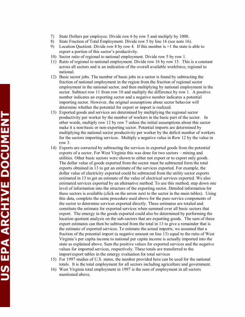
7) State Dollars per employee. Divide row 6 by row 5 and multiply by 1000. 8) State Fraction of Total Employment. Divide row 5 by line 16 (see note 16). 9) Location Quotient. Divide row 8 by row 4. If this number is >1 the state is able to

export a portion of this sector’s productivity. 10) Sector ratio of regional to national employment. Divide row 5 by row 1. 11) Ratio of regional to national employment. Divide row 16 by row 15. This is a constant

across all sectors and is an indication of the overall available workforce, regional to national.

12) Basic sector jobs. The number of basic jobs in a sector is found by subtracting the fraction of national employment in the region from the fraction of regional sector employment in the national sector, and then multiplying by national employment in the sector. Subtract row 11 from row 10 and multiply the difference by row 1. A positive number indicates an exporting sector and a negative number indicates a potential importing sector. However, the original assumptions about sector behavior will determine whether the potential for export or import is realized.

13) Exported goods and services are determined by multiplying the regional sector productivity per worker by the number of workers in the basic part of the sector. In other words, multiply row 12 by row 7 unless the initial assumptions about this sector make it a non-basic or non-exporting sector. Potential imports are determined by multiplying the national sector productivity per worker by the deficit number of workers for the sectors importing services. Multiply a negative value in Row 12 by the value in row 3.

14) Exports are corrected by subtracting the services in exported goods from the potential exports of a sector. For West Virginia this was done for two sectors – mining and utilities. Other basic sectors were shown to either not export or to export only goods. The dollar value of goods exported from the sector must be subtracted form the total exports obtained in 13 to get an estimate of the services exported. For example, the dollar value of electricity exported could be subtracted from the utility sector exports estimated in 13 to get an estimate of the value of electrical services exported. We also estimated services exported by an alternative method. To use this method, step down one level of information into the structure of the exporting sector. Detailed information for these sectors is available (click on the arrow next to the sector in the main tables). Using this data, complete the same procedure used above for the pure service components of the sector to determine services exported directly. These estimates are totaled and constitute the estimate for exported services when summed over all basic sectors that export. The emergy in the goods exported could also be determined by performing the location quotient analysis on the sub-sectors that are exporting goods. The sum of these export estimates can then be subtracted from the total in 13 to give a remainder that is the estimate of exported services. To estimate the actual imports, we assumed that a fraction of the potential import (a negative amount on line 13) equal to the ratio of West Virginia’s per capita income to national per capita income is actually imported into the state as explained above. Sum the positive values for exported services and the negative values for imported services, respectively. These totals are transferred to the import/export tables in the emergy evaluation for total services

15) For 1997 studies of U.S. states, the number provided here can be used for the national totals. It is the total employment for all sectors including agriculture and government.

16) West Virginia total employment in 1997 is the sum of employment in all sectors mentioned above.

Appendix E.

West Virginia Emergy Accounts for 2000.

Table E1 Renewable Resources and Production in the West Virginia Economy in 2000.

Note Item Data J, g, $, ind/yr

Units Emergy/Unit sej/unit

Emergy E20 sej

2000 Emdollars E6 Em$

Renewable Resources within West Virginia 1 Sun, incident 3.074 E+20 J 1 3 2871 Sun, absorbed 2.644 E+20 J 1 3 2472 Wind 3.580 E+17 J 1470 5.3 4393 Earth Cycle 1.388 E+17 J 33700 47 43724 Rain, chemical potential energy received 3.323 E+17 J 18100 60 56215 Evapotranspiration, chemical potential absorbed 1.561 E+17 J 28100 44 40996 Rain, geo-potential on land 3.655 E+17 J 10300 38 35187 Rain, geo-potential of runoff 6.024 E+16 J 27200 16 15318 Rivers, chemical potential energy received 9.056 E+16 J 50100 45 42408 Rivers, chemical potential energy absorbed 2.896 E+14 J 50100 0.15 149 Rivers, geo-potential energy received 4.987 E+16 J 27200 14 12689 Rivers, geo-potential energy absorbed 2.058 E+16 J 27200 5.6 523

Renewable Production within West Virginia 10 Agricultural Products 5.340 E+16 J 50000 27 249511 Livestock

Beef 6.932 E+14 J 680000 4.7 441 All other livestock 3.970 E+14 J 792000 3.1 294

12 Fish Production 7.099 E+11 J 1961800 0.14 113 Hydroelectricity 1.092 E+16 J 120300 13 122814 Net Timber Growth 2.096 E+17 J 20600 43 403515 Timber harvest 2.286 E+16 J 68700 16 146816 Ground water 9.493 E+14 J 159000 1.5 141

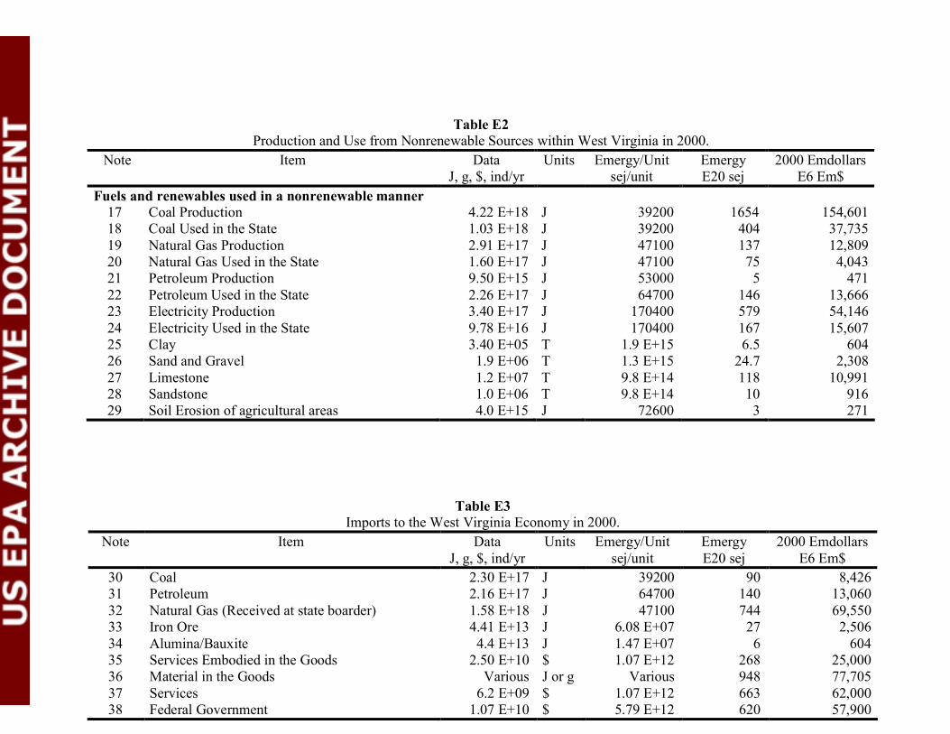
Table E2 Production and Use from Nonrenewable Sources within West Virginia in 2000.

Note Item Data J, g, $, ind/yr

Units Emergy/Unit sej/unit

Emergy E20 sej

2000 Emdollars E6 Em$

Fuels and renewables used in a nonrenewable manner 17 Coal Production 4.22 E+18 J 39200 1654 154,60118 Coal Used in the State 1.03 E+18 J 39200 404 37,73519 Natural Gas Production 2.91 E+17 J 47100 137 12,80920 Natural Gas Used in the State 1.60 E+17 J 47100 75 4,04321 Petroleum Production 9.50 E+15 J 53000 5 47122 Petroleum Used in the State 2.26 E+17 J 64700 146 13,66623 Electricity Production 3.40 E+17 J 170400 579 54,14624 Electricity Used in the State 9.78 E+16 J 170400 167 15,60725 Clay 3.40 E+05 T 1.9 E+15 6.5 60426 Sand and Gravel 1.9 E+06 T 1.3 E+15 24.7 2,30827 Limestone 1.2 E+07 T 9.8 E+14 118 10,99128 Sandstone 1.0 E+06 T 9.8 E+14 10 91629 Soil Erosion of agricultural areas 4.0 E+15 J 72600 3 271

Table E3 Imports to the West Virginia Economy in 2000.

Note Item Data J, g, $, ind/yr

Units Emergy/Unit sej/unit

Emergy E20 sej

2000 Emdollars E6 Em$

30 Coal 2.30 E+17 J 39200 90 8,42631 Petroleum 2.16 E+17 J 64700 140 13,06032 Natural Gas (Received at state boarder) 1.58 E+18 J 47100 744 69,55033 Iron Ore 4.41 E+13 J 6.08 E+07 27 2,50634 Alumina/Bauxite 4.4 E+13 J 1.47 E+07 6 60435 Services Embodied in the Goods 2.50 E+10 $ 1.07 E+12 268 25,00036 Material in the Goods Various J or g Various 948 77,70537 Services 6.2 E+09 $ 1.07 E+12 663 62,00038 Federal Government 1.07 E+10 $ 5.79 E+12 620 57,900

Table E4 Exports from the West Virginia Economy in 2000.

Note Item Data J, g, $, ind/yr

Units Emergy/Unit sej/unit

Emergy E20 sej

2000 Emdollars E6 Em$

39 Coal 3.19 E+18 J 39200 1250 116,86740 Natural Gas (Production Exports) 1.20 E+17 J 47100 57 5,28241 Natural Gas (Delivered at state border) 1.75 E+18 J 47100 824 77,03242 Electricity 2.42 E+17 J 170400 412 38,53943 Steel 2.00 E+12 g 3.38 E+09 68 6,31744 Services Embodied in the Goods 2.72 E+10 $ 1.07 E+12 291 27,20045 Material in the Goods Various J or g Various 776 72,52346 Services 5.80 E+08 $ 1.07 E+12 6 58047 Migration (total) 2660 People Various 4.2 344

Preschool 876 People 3.3 E+16 0.3 24 School 1188 People 9.2 E+16 1.1 90 College Grad 479 People 2.7 E+17 1.29 106 Post-College 117 People 1.3 E+18 1.5 125

48 Tourism 4.0 E+09 $ 5.79 E+12 232 21,68238 Federal Taxes Paid 6.1 E+09 $ 5.79 E+12 353 32,990

Table E5 Value of West Virginia Storages in 2000.

Note Item Data J, g, $, ind/yr

Units Emergy/Unit sej/unit

Emergy E20 sej

2000 Emdollars E6 Em$

49 Forest 1.04 E+19 J 28200 2933 274,09350 Coal 1.42 E+21 J 39200 556640 52,022,42951 Petroleum 1.19 E+17 J 53000 63 5,89452 Natural Gas 3.13 E+18 J 47100 1474 137,77953 People 2000 population 1,808,344 Ind. 3908 365,394

Preschool 21,635 Ind. 3.3 E+16 7 667 School 1,164,463 Ind. 9.2 E+16 1071 100,122 College Grad 384,232 Ind. 2.7 E+17 1037 96,955 Post-College 56,266 Ind. 1.3 E+18 731 68,360 Elderly (70+) 163,101 Ind. 1.7 E+17 277 25,913 Public Status 18,568 Ind. 3.9 E+18 724 67,678 Legacy 792 Ind. 7.7 E+18 61 5,699

Table E6 Summary of Flows for West Virginia in 2000.

Note Letter in Fig.

2

Item Emergy E20 sej

1997 Dollars E+09 $/yr

2000 Emdollars

E+09 Em$/y

54 RR Renewable emergy received 105 9.8254 RA Renewable emergy absorbed 66 6.1755 N Nonrenewable source flows 1958 182.9956 N0 Dispersed Rural Source 3 0.28 57 N1 Mineral Production (fuels, etc.) 1955 182.71 58 N2 Fuels Exported without Use 1312 122.6259 F Imported Minerals (fuels, etc.) 263 24.5860 F1 Minerals Used (F+N1-N2) 906 84.6761 F2 In State Minerals Used (N1-N2) 643 60.0962 G Imported Goods (materials) 948 88.6063 I Dollars Paid for all Imports 31.13 64 I1 Dollars Paid for Service in Fuels 1.72 65 I2 Dollars Paid for Service in Goods 23.24 66 I3 Dollars paid for Services 6.17 67 I6 Federal Transfer Payments 10.7 68 PI Imported Services Total 375 35.0569 PI1 Imported Services in Fuels 21 1.9670 PI2 Imported Services in Goods 280 26.1771 PI3 Imported Services 74 6.9272 PI4 Emergy purchased by Federal $ 620 57.9473 B Exported Products (goods + elec.) 1188 111.0374 E Dollars Paid for Exports 31.08 75 E1 Dollars Paid Fuel Exported 3.92 76 E2 Dollars Paid for Goods 26.6 77 E3 Dollars Paid for Exported Services 0.58 78 E4 Dollars Spent by Tourist 4.0 79 E5 Federal Taxes Paid 6.1 80 PE Total Exported Services 379 35.4281 PE1 Exported Services in Fuels 48 4.4982 PE2 Exported Services in Goods 324 30.2883 PE3 Exported Services 7 0.6584 PE4 Emergy Purchased by Tourists 237 22.1585 PE5 Emergy Purchases Forgone 353 32.9986 X Gross State Product 39.7