Weak Bisimulation for Fully Probabilistic

Processes

Christel Baier a and Holger Hermanns b

a Fakultat fur Mathematik & Informatik, Universitat Mannheim,Seminargebaude A 5, 68131 Mannheim, Germany

baier@pi2.informatik.uni-mannheim.deb Systems Validation Centre, FMT/CTIT, University of Twente,

P.O. Box 217, 7500 AE Enschede, The Netherlandshermanns@cs.utwente.nl

Abstract

Bisimulations that abstract from internal computation have proven to be usefulfor verification of compositionally defined transition systems. In the literature ofprobabilistic extensions of such transition systems, similar bisimulations are rare.In this paper, we introduce weak and branching bisimulation for fully probabilisticsystems, transition systems where nondeterministic branching is replaced by proba-bilistic branching. In contrast to the nondeterministic case, both relations coincide.We give an algorithm to decide weak (and branching) bisimulation with a time com-plexity cubic in the number of states of the fully probabilistic system. This meets theworst case complexity for deciding branching bisimulation in the nondeterministiccase. In addition, the relation is shown to be a congruence with respect to the op-erators of PLSCCS , a lazy synchronous probabilistic variant of CCS. We illustratethat due to these properties, weak bisimulation provides all the crucial ingredientsfor mechanised compositional verification of probabilistic transition systems.

Centre for Telematics and Information Technology TR-CTIT-12, June 1999

Contents

1 Introduction 3

2 Fully probabilistic systems 6

3 Weak and branching bisimulation 9

3.1 Weak bisimulation 9

3.2 Branching bisimulation 11

3.3 Connection to other equivalences 14

4 Deciding weak bisimulation equivalence 18

4.1 The algorithm 19

4.2 Complexity of the algorithm 25

5 Lazy synchronous CCS 27

5.1 PLSCCS : a lazy synchronous calculus 29

5.2 Compositionality 35

6 Putting it all together 37

7 Conclusion 39

A Proofs of the main theorems 41

A.1 Weak and branching bisimulation 41

A.2 Weak bisimulation and the testing equivalences =ste and ≡0 51

References 57

2

1 Introduction

In recent years, the need to formally reason about probabilistic phenomena insoftware and hardware systems has stimulated the study of probabilistic mod-els of computation. A variety of models has been proposed in the literature,many of them based on transition systems. These models can be classifiedwith respect to their treatment of nondeterminism. Several approaches re-place the concept of nondeterministic branching by probabilistic branching,e.g. [19,33,48,73,27]. Following [27], this model can be subdivided accordingto the relationship between occurrences of actions and transition probabili-ties. In ’reactive’ systems, transition probability distributions are dependenton the occurrences of actions. In contrast, in ’generative’ – also called fullyprobabilistic – systems, these distributions implicitly assign probabilities alsoto occurrences of actions. ’Stratified’ systems allow for levelwise probabilisticbranching. Other authors, e.g. [71,60,32,44,64], allow for both, nondeterminis-tic as well as probabilistic branching, mainly because this allows one to expressthe concurrent (interleaved) execution of independent (probabilistic) activitiesby means of nondeterminism. Accordingly, we subsume these models as con-current probabilistic systems.

Verification techniques for probabilistic models have been inspired by suc-cessful experiences in the non-probabilistic case. This includes probabilisticvariants of temporal logics, e.g. [4,12,21,32–34,60,61,71,72]. Another researchstrand focusses on equivalences and preorders used to established that one sys-tem ’implements’ another, according to some notion of implementation, suchas strong bisimulation [48], simulation [41,64], testing preorders [19,44,74,73],trace, failure and ready equivalence [43].

In the context of specification and verification of distributed (non-probabilistic) systems, weak [58,53] or branching [28] bisimulation are thebasis for a variety of verification methods because of three crucial properties.These equivalences (1) exploit abstraction from internal computation, theyare (2) compositional with respect to parallel composition and other opera-tors, and (3) efficient algorithms exist to minimise components with respect totheir internal behaviour [57,45]. In this way, the omnipresent phenomenon ofstate-space explosion can be alleviated. Instead of building the global transi-tion system underlying some (specification or) implementation, the transitionsystem is built up componentwise, where weak (or branching) bisimulation al-gorithms are applied to minimise the intermediate state spaces of components.This can enormously reduce the size of the global transition system withoutaffecting properties to be verified. An impressive example of this strategy isgiven in [14].

Several authors mentioned that the definition of a weak bisimulation that

3

abstracts from internal computation is desirable, but problematic in a prob-abilistic setting [43,32]. Segala&Lynch [64,65] introduce notions of weak andbranching bisimulation for concurrent probabilistic systems. Their definitionof weak and branching bisimulation replaces Milner’s weak transition relationα

=⇒ (which is defined with the help of the transitive, reflexive closure (τ−→)∗

of internal transitions) by assigning a (possibly infinite) set of distributions toeach state. Their definitions are natural extensions of non-probabilistic weakand branching bisimulation to probabilistic systems with non-determinism(concurrent probabilistic systems) but it is not obvious how a definition forthe fully probabilistic case can be derived.

In this paper, we introduce notions of weak bisimulation and branching bisim-ulation for fully probabilistic systems that arise as rather natural extensionsof the corresponding relations in the non-probabilistic case. The basic ideais to replace Milner’s weak transitions s

α=⇒ t ( i.e. s(

τ−→)∗α−→ (

τ−→)∗t)by the probabilities to reach state t from s via a sequence of transitions la-belled by a trace of the form τ ∗ατ ∗. In contrast to the non-probabilistic casewhere branching bisimulation equivalence is strictly finer than weak bisimu-lation equivalence, the two equivalences coincide for finite fully probabilisticsystems. Moreover, we show that this notion of equivalence enjoys a centralposition relative to other weak relations for fully probabilistic systems foundin the literature.

For mechanised verification purposes, the decidability of such equivalences,together with efficient algorithms for finite state systems is a crucial aspect.In the non-probabilistic case, for instance, strong bisimulation can be decidedin time O(m · log n) [57] where n is the number of states and m the number oftransitions in the underlying (finite) transition system. Weak bisimulation canbe computed by means of the same algorithm, but on an induced transitionsystem where the weak relation =⇒ replaces the strong relation −→. In otherwords, the problem of deciding (or minimising with respect to) weak bisimula-tion is reduced to the computation of the transitive, reflexive closure (

τ−→)∗ ofinternal transitions and deciding strong bisimulation in a finite system. Usingthe transitive closure operation from [20] and the partitioning/splitter tech-nique by [57] the time complexity for deciding weak bisimulation is O(n2.3)where n is the number of states. For computing branching bisimulation of anon-probabilistic system, Groote&Vaandrager [30] propose an algorithm whichworks with a variant of the partitioning/splitter technique a la [45]. It usesboth transition relations (−→ and =⇒), and runs in time O(nm) where n isthe number of states and m the number of transitions, i.e. the size of −→.

As far as the authors know, the question whether weak or branching bisimula-tion on concurrent probabilistic systems (i.e. in the style of [64,65]) is decidableis still open, even though some effort in this direction has been carried outrecently [59,9]. The main problem appears to be that the induced weak transi-

4

tion relation =⇒ might be infinite, even for finite systems; hence, an adaptionof the methods used in the non-probabilistic case fails. However, we showthat in the fully probabilistic case, weak (or branching) bisimulation equiva-lence is decidable for finite systems. We present an algorithm to compute theweak bisimulation equivalence classes with a modification of the partition-ing/splitter technique a la [45,57]. The time complexity of our method is cubicin the number of states; thus, it meets the worst case complexity for decidingbranching bisimulation in the non-probabilistic case [30] (where, in the worstcase, O(m) = O(n2)).

This provides us with an equivalence that (1) exploits abstraction from in-ternal computation together with (3) an efficient algorithm to minimise com-ponents with respect to their internal behaviour. In order to cover all threemain ingredients of a compositional verification method for fully probabilisticsystems, we introduce a probabilistic calculus, PLSCCS . The calculus pro-vides the standard CCS-style operators to specify systems, where probabilis-tic choice replaces non-deterministic choice, and parallel composition is lazysynchronous. Lazy synchrony refers to a form of synchronisation, where visi-ble actions are forced to proceed in lockstep, i.e. synchronously, while internalactions are supposed to happen locally in some component, and hence areexcluded from synchronisation, they happen asynchronously. Similar kinds ofcomposition are present in synchronous languages, such as Esterelle [11], Lus-tre [31], or others [18,13,36]. We show that weak and branching bisimulationare congruences with respect to the operators of PLSCCS , with the exception(inherited from the non-probabilistic setting) of the probabilistic choice oper-ator. So, PLSCCS provides means for a compositional specification of fullyprobabilistic systems. In addition, the algorithm for weak bisimulation canbe used to minimise components of a complex fully probabilistic system withrespect to their internal behaviour, without affecting properties to be verified.

Organisation of the paper: In Section 2 we introduce the fully probabilisticmodel together with basic notations used in the sequel. Section 3 introducesweak and branching bisimulation, and shows that both coincide for finite sys-tems, It also discusses the relation between weak (and branching) bisimulationand other equivalences for fully probabilistic systems found in the literature.In Section 4 we present our algorithm for deciding weak bisimulation. Section5 is devoted to the calculus PLSCCS and the proof of congruence. In Section 6we illustrate how the congruence property and the algorithm can be exploitedfor a compositional verification technique. Section 7 concludes the paper. Toenhance readability, most of the proofs are given in the appendix.

5

2 Fully probabilistic systems

In this section we introduce the fully probabilistic model, the model we fo-cus on throughout this paper. It can be regarded as a specialisation of non-probabilistic transition systems where probabilities are used to resolve nonde-terminism. From a slightly different point of view, it can also be interpretedas an action-labelled Markov chain with discrete parameter set [46].

In non-probabilistic labelled transition systems, the possible steps from statesto successor states are described by a transition relation −→ ⊆ S ×Act × S(where Act stands for the underlying set of actions), i.e. the state changesare associated with action labels. Intuitively, s

a−→t asserts that, in state s,it is possible to perform the action a and to reach state t afterwards. Theprobability of choosing one particular transition is unspecified. In contrast,fully probabilistic systems quantify the probability of each possible transitionby means of a transition probability function P, where P(s, a, t) determinesthe probability to perform the action a from state s and to reach t in doingso.

We first introduce some standard notations for actions and action sequences.For L ⊆ Act , L∗ denotes the set of finite sequences over L. The empty sequenceis denoted by ε. L+ denotes the set of finite nonempty sequences over Act ,i.e. L+ = L∗ \ ε. We further assume that Act contains a distinguishedsymbol τ . Intuitively, τ stands for any ’internal’ activity of the system whichis invisible for an observer (or the environment of the system). We refer toτ as the internal action. The other actions are called visible. We use greekletters α, β, . . . to denote visible actions and arabic letters a, b, . . . to rangeover arbitrary actions.

Definition 2.1 A fully probabilistic system is a tuple (S,Act ,P) consistingof a set S of states, a nonempty set Act of actions and a function P : S ×Act × S −→ [0, 1] (called the transition probability function) such that, foreach s ∈ S, P(s, a, t) > 0 for at most countably many pairs (a, t) ∈ Act × Sand

∑a,t P(s, a, t) ∈ 0, 1.

Let (S,Act ,P) be a fully probabilistic system. S is said to be finite iff S andAct are finite. A state s of S is called terminal iff

∑a,t P(s, a, t) = 0.

Example 2.2 We consider a simple communication protocol similar to thatin [33]. The system consists of two entities: a sender working with an unreli-able medium to transmit messages to a receiver. The sender, having produceda message, passes the message to the medium, which in turn tries to deliverit to the receiver. With probability 0.01, the messages gets lost, in this casethe medium retries to deliver it correctly. With probability 0.99, the messageis delivered correctly. Once this has occured the sender waits for the acknowl-

6

sinit

sdel

slostswait

send !, 1

ack?, 1

τ , 0.99

τ , 0.01

τ , 1

?

'-

JJJJ

JJ

JJJJ

JJ]

Fig. 1. The sender with action labels

edgement from the receiver’s side and then returns to the initial state. Forsimplicity, we assume that the acknowledgement cannot be corrupted or lost.We describe the behaviour of the sender by the fully probabilistic system de-picted in Figure 1, using four states:

• sinit : the state in which the sender produces a message and passes the mes-sage to the medium. This is modelled by an output action (send !).

• sdel : the state in which the medium tries to deliver the message,• slost : the state reached when the message is lost, and retransmission is nec-

essary,• swait : the state reached when the message is delivered correctly and in which

the system waits for the acknowledgement by the receiver, modelled by aninput action (ack?).

For instance, the transition swaitack?−→ sinit stands for the case where the sender

gets the acknowledgement of the receipt of the message; sdelτ−→ slost for

the case where the medium looses the messages. This event, as well as re-transmission and correct delivery, is supposed to be invisible from the pointof view of the sender. In total, the behaviour of the sender can be specifiedby the fully probabilistic system (S,Act ,P) where S = sinit , sdel , slost , swaitand P(sinit , send !, sdel) = P(slost , τ, sdel) = P(swait , ack?, sinit) = 1,P(sdel , τ, sinit) = 0.01, P(sdel , τ, swait) = 0.99 and P(·) = 0 in all other cases.

For s ∈ S, C ⊆ S, a ∈ Act and L ⊆ Act , we define P(s, a, C) =∑t∈C P(s, a, t), P(s, a) = P(s, a, S), and P(s, L) =

∑a∈L P(s, a). An exe-

cution fragment or finite path is a nonempty finite sequence

σ = s0a1−→ s1

a2−→ s2a2−→ . . .

ak−→ sk

such that s0, s1, . . . , sk ∈ S, a1, . . . , ak ∈ Act and P(si−1, ai, si) > 0, i =1, . . . , k. We use following notations,

• |σ| denotes the length of σ, i.e. |σ| = k.• first(σ) denotes the first state of σ, i.e. first(σ) = s0.• last(σ) denotes the last state of σ, i.e. last(σ) = sk.

7

• σ(i) denotes the (i+ 1)-st state of σ, i.e. σ(i) = si, i = 0, 1, . . . , k.• σ(i) denotes the i-th prefix of σ, i.e. σ(i) = s0

a1−→ s1a2−→ . . .

ai−→ si,i = 0, 1, . . . , k. If i > k = |σ| then we let σ(i) = σ.• trace(π) = a1a2 . . . ak.• If k = |σ| = 0 then we put P(σ) = 1. For k ≥ 1, we define

P(σ) = P(s0, a1, s1) ·P(s1, a2, s2) · . . . ·P(sk−1, ak, sk).

• σ is called maximal iff last(σ) is terminal.• state t is called reachable from state s if there exists a finite path σ with

first(σ) = s and last(σ) = t.

Example 2.3 For the system in Example 2.2, σ = sinitsend!−→ sdel

τ−→slost

τ−→ sdelτ−→ swait is an execution fragment (finite path) with |σ| = 4,

first(σ) = sinit , last(σ) = swait , σ(2) = slost , σ(2) = sinit −→ sdel −→ slost and

P(σ) = 1 · 0.01 · 1 · 0.99 = 0.0099. It has no finite maximal execution fragmentas there are no terminal states.

An execution or fulpath in (S,Act ,P) is either a maximal execution fragmentor an infinite sequence π = s0

a1−→ s1a2−→ s2

a2−→ . . . where s0, s1, . . . ,∈S, a1, a2, . . . ∈ Act and P(si−1, ai, si) > 0, i = 1, 2, . . .. A path denotes anexecution fragment or an execution. For path π to be an infinite sequence, π(i),π(i) and first(π) are defined as for execution fragments, trace(π) = a1a2 . . .,|π| =∞, and we define

inf (π) = s ∈ S : π(i) = s for infinitely many indices i ≥ 0.

If, on the other hand, σ is a finite path then we define inf (σ) = ∅.

Example 2.4 For the system of Figure 1,

π = sinitsend !−→ sdel

τ−→ slostτ−→ sdel

τ−→ slostτ−→ . . .

is an execution (fulpath) with π(2) = sinitsend !−→ sdel

τ−→ slost , first(π) = sinit ,π(3) = sdel , P(π(4)) = 1 ·0.01 ·1 ·0.01 = 0.0001 and trace(π(4)) = send ! τ τ τ .

We let PathSful (PathSful(s)) denote the set of fulpaths in S (starting in state

s). Similarly, PathSfin (PathSfin(s)) denotes the set of finite paths in S (startingin state s). The set of states which are reachable from s are subsumed inReachS(s). If the underlying fully probabilistic system S is clear from thecontext we usually omit the superscript S. For each state s, P induces aprobability space on Path ful(s) as follows. Let σ ↑ denote the basic cylinderinduced by σ, i.e.

σ ↑ = π ∈ Path ful(s) : σ ≤prefix π .

where ≤prefix is the usual prefix relation on paths. We define σFieldS(s) to

8

be the smallest sigma-field on Path ful(s) which contains all basic cylindersσ ↑ where σ ∈ Pathfin(s), i.e. σ ranges over all finite paths starting ins. The probability measure Prob on σFieldS(s) is the unique measure withProb (σ ↑) = P(σ).

Lemma 2.5 Let (S,Act ,P) be a fully probabilistic system and Σ ⊆ Pathfin

such that σ, σ′ ∈ Σ, σ 6= σ′ implies σ 6≤prefix σ′. Then, for all s ∈ S,

Prob (Σ(s) ↑) =∑

σ∈Σ(s)

P(σ).

3 Weak and branching bisimulation

In this section we define weak and branching bisimulation for fully probabilis-tic systems. While in the non-probabilistic case branching bisimulation equiv-alence is strictly finer than weak bisimulation equivalence, these two relationscoincide for finite fully probabilistic systems (Theorem 3.9). As a startingpoint, we recall strong probabilistic bisimulation, an elegant generalisation ofnon-probabilistic bisimulation [51,58]. Originally introduced by Larsen&Skou[48] for reactive systems, it has been reformulated by van Glabbeek et al [27]for fully probabilistic systems.

Definition 3.1 A strong bisimulation on a fully probabilistic system(S,Act ,P) is an equivalence relation R on S such that (s, s′) ∈ R impliesfor all a ∈ Act and all C ∈ S/R.

P(s, a, C) = P(s′, a, C)

Two states s, s′ are called strongly bisimulation equivalent (denoted s ∼ s′)iff (s, s′) ∈ R for some strong bisimulation R.

3.1 Weak bisimulation

In order to abstract from internal moves, non-probabilistic weak bisimulationneglects these moves as far as they do not influence the future behaviour ofa process. To do so, Milner [53] introduces a notion of observable steps of aprocess, that consist of a single visible action α preceded and followed by anarbitrary number (including zero) of internal steps. Technically this is achievedby deriving a ’weak’ transition relation =⇒ from the ’strong’ relation −→, bysetting

α=⇒ = (

τ−→)∗α−→ (

τ−→)∗, andτ

=⇒= (τ−→)∗. Note that a weak internal

transitionτ

=⇒ is possible without actually performing an internal action.

9

For the definition of weak bisimulation in the fully probabilistic setting, we re-place Milner’s weak internal transitions s

τ=⇒ t by the probability Prob(s, τ ∗, t)

to reach state t from s via internal actions. Similarly, for visible actions α. wedeal with the probabilities Prob(s, τ ∗ατ ∗, t) rather than the weak transitionrelation

α=⇒.

Definition 3.2 A weak bisimulation on a fully probabilistic system(S,Act ,P) is an equivalence relation R on S such that (s, s′) ∈ R impliesfor all a ∈ Act and all C ∈ S/R:

(1) Prob(s, τ ∗, C) = Prob(s′, τ ∗, C)(2) Prob(s, τ ∗ατ ∗, C) = Prob(s′, τ ∗ατ ∗, C) for all α ∈ Act \ τ.

Two states s, s′ are called weakly bisimulation equivalent (denoted s ≈ s′)iff (s, s′) ∈ R for some weak bisimulation R.

Note that Prob(s, τ ∗, C) = 1 if s ∈ C. Hence, condition (1) is always fulfilledfor the equivalence class C of s (and s′). It is easy to see that any strongbisimulation is a weak bisimulation, and hence ∼ ⊆ ≈.

Lemma 3.3 For finite systems, ≈ is a weak bisimulation.

The proof is given in the appendix (cf. Lemma A.17).

Example 3.4 We compare the fully probabilistic system describing thesender’s behaviour shown in Figure 1 with a simple specification of a com-munication protocol depicted below.

s′init

s′wait

send !, 1ack?, 1

6

?

Using weak bisimulation equivalence as the underlying implementation relationthe sender can be verified against this specification. To illustrate this, we showthat the initial states sinit and s′init are weakly bisimulation equivalent. Let Rbe the equivalence on S = sinit , sdel , swait , slost , s

′init , s

′wait such that S/R =

CI , CW where CI = sinit , s′init is the equivalence class of the initial states

and CW = sdel , swait , slost , s′wait the equivalence class of the other states. For

10

sI ∈ CI and sW ∈ CW , we have:

Prob(sI , τ∗, CI) = 1, Prob(sW , τ

∗, CI) = 0,

Prob(sI , τ∗, CW ) = 0, Prob(sW , τ

∗, CW ) = 1,

Prob(sI , τ∗ send ! τ ∗, CI) = 0, Prob(sW , τ

∗ send ! τ ∗, CI) = 0,

Prob(sI , τ∗ ack? τ ∗, CI) = 0, Prob(sW , τ

∗ ack? τ ∗, CI) = 1,

Prob(sI , τ∗ send ! τ ∗, CW ) = 1, Prob(sW , τ

∗ send ! τ ∗, CW ) = 0,

Prob(sI , τ∗ ack? τ ∗, CW ) = 0, Prob(sW , τ

∗ ack? τ ∗, CW ) = 0.

Hence, R is a weak bisimulation. In particular, the initial states sinit of thesender and s′init of its specification are weakly bisimulation equivalent.

In the non-probabilistic case, it holds for weakly bisimulation equivalentstates s, s′ that if s

α1...αk=⇒ t then there is some t′ such that s′α1...αk=⇒

t′, and that t, t′ are weakly bisimulation equivalent. Here,α1...αk=⇒ denotes

(τ−→)∗

α1−→ (τ−→)∗ . . . (

τ−→)∗αk−→ (

τ−→)∗. This result carries over to finite fullyprobabilistic systems.

Theorem 3.5 Let (S,Act ,P) be a finite fully probabilistic system and Ω aregular expression of the form τ ∗α1τ

∗α2τ∗ . . . τ ∗αk or τ ∗α1τ

∗α2τ∗ . . . τ ∗αkτ

∗.Then:

If s ≈ s′ then Prob(s, Ω, C) = Prob(s′, Ω, C) for all C ∈ S/ ≈.

Proof: see Section A.1, Theorem A.18.

3.2 Branching bisimulation

From a specific point of view, non-probabilistic weak bisimulation appearstoo coarse. Strong bisimulation has the property that any computation in oneprocess corresponds to a computation in the other in such a way that allintermediate steps correspond as well. This is not true for weak bisimulation.The standard counterexample (taken from [28]) is depicted in Figure 2. In thisexample, s and s′ are weakly bisimulation equivalent, but the computations

sα

=⇒ tβ

=⇒ w and s′α

=⇒ v′′β

=⇒ w′′ pass through intermediate states (t andv′′) that are not equivalent. In particular, the latter computation does not passthrough any state where γ is possible.

In order to overcome this lack, van Glabbeek&Weijland postulate a branchingcondition [28]. The basic idea is that in order to simulate a step s

α−→ t byan equivalent state s′ with a sequence s′

τ=⇒ α−→ τ

=⇒ t′, all steps preceding

11

w

v u

t

s

w′

v′ u′

t′

s′

v′′

w′′

α

τ γ

β

α

τ γ

β

α

β

@@@R?

?

?

?

AAAU

AAAU

Fig. 2. Distinguishing weak and branching bisimulation in the non-probabilisticcase

the transitionα−→ have to remain inside the equivalence class of s (and s′)

and all steps following this transition have to stay inside the class of t (andhence of t′). To achieve this property it is sufficient to demand that s′ performsarbitrarily many internal actions leading to a state s′′ which is still equivalentto s′ (and s) and then to directly reach the equivalence class of t by performingaction α. This implies that all intermediate states on the path from s′ to s′′

also belong to equivalence class of s′, s, and s′′ [28].

To adapt this idea to the fully probabilistic case, we deal with the probabilityto reach an equivalence class C (of a given equivalence relation R) from astate s by means of a trace labelled τ ∗α, where the τ steps only pass throughstates equivalent to s (with respect to R). This probability will be denotedProbR(s, τ ∗α,C), and is defined below. For notational convenience, we shalluse τ to denote ε, whereas for visible actions, α = α. Recall that ε denotesthe empty word in Act∗. Hence, τ ∗a = τ ∗ if a = τ .

Definition 3.6 Let (S,Act ,P) be a fully probabilistic system, R an equiva-lence relation on S, s ∈ S, C ⊆ S and a ∈ Act. Then, PathRful(s, τ

∗a, C)denotes the set of fulpaths π ∈ Path ful(s) such that there is some k ≥ 0 with

• (s, π(i)) ∈ R, i = 1, . . . , k − 1,• trace(π(k)) ∈ τ ∗a,• π(k) ∈ C.

Let ProbR(s, τ ∗a, C) = Prob(PathRful(s, τ∗a, C)), and furthermore

ProbR(s, τ ∗a, t) = Prob((s, τ ∗a, t).

Example 3.7 The reader is invited to check that for the relation R in Ex-ample 3.4, we have ProbR(s, τ ∗aτ ∗, C) = Prob(s, τ ∗aτ ∗, C) for all states s,classes C ∈ CI , CW and a ∈ τ, send !, ack?.

12

v

ut

s

α, 1

2τ , 12

β, 1?

@@@R

For the system shown above and the (identity) relation R with (x, y) ∈ R iffx = y, we have ProbR(s, τ ∗β, v) = 0 while Prob(s, τ ∗β, v) = 1/2.

It is worth noticing that for arbitrary equivalences R on S, and C ⊆ S, s ∈ Cimplies Path ful(s) = PathRful(s, τ

∗, C), and hence ProbR(s, τ ∗, C) = 1 if s ∈ C.We now have the necessary means to lift branching bisimulation to the fullyprobabilistic case.

Definition 3.8 Let (S,Act ,P) be a fully probabilistic system. A branchingbisimulation on (S,Act ,P) is an equivalence relation R on S such that for all(s, s′) ∈ R, C ∈ S/R:

(1) ProbR(s, τ ∗, C) = ProbR(s, τ ∗, C)(2) ProbR(s, τ ∗α,C) = ProbR(s, τ ∗α,C) for all α ∈ Act \ τ.

Two states s, s′ are called branching bisimulation equivalent (denoted s ≈br s′)iff (s, s′) ∈ R for some branching bisimulation R.

For finite systems, branching bisimulation equivalence ≈br is a branchingbisimulation, as shown in the appendix (cf. Lemma A.16). In contrast to thenon-probabilistic case, where branching bisimulation equivalence is strictlyfiner than weak bisimulation equivalence, the branching condition does notadd any distinguishing power to the relation in the fully probabilistic setting;weak and branching bisimulation equivalence coincide for finite systems:

Theorem 3.9 Let (S,Act ,P) be a finite fully probabilistic system and s, s′ ∈S. Then, s ≈ s′ iff s ≈br s′.

Proof: The proof is given in the appendix (cf. Corollary A.14).

To exemplify the difference to the non-probabilistic setting, we return tothe standard example depicted in Figure 2. In the non-probabilistic case,s and s′ are weakly but not branching bisimulation equivalent. However, ifwe add non-zero probabilities (which turns the system into a fully proba-bilistic system) then s and s′ are neither branching, nor weakly bisimulationequivalent. This can be seen as follows. Assume that s ≈ s′ holds. Then,1 = Prob(s, τ ∗ατ ∗, T ) = Prob(s′, τ ∗ατ ∗, T ) has to hold, where T de-notes the weak bisimulation equivalence class of t. Clearly, v′′ does not be-long to T , because t can perform γ (with non-zero probability) while v′′ can-

13

not. Hence Prob(s′, τ ∗ατ ∗, T ) = 1 implies P(s′, α, t′) = 1, and thereforeP(s′, α, v′′) = 0. This contradicts our decision to add non-zero probabilitiesto the non-probabilistic system of Figure 2, in particular transition s′

α−→ v′′.

3.3 Connection to other equivalences

In this section we discuss how weak (and branching) bisimulation relates toother equivalences for fully probabilistic systems studied in the literature.First, it is not surprising that weak bisimulation equivalence ≈ is strictlycoarser than strong bisimulation equivalence ∼ (Definition 3.1) since the lat-ter does not abstract from internal moves. Formally, if (S,Act ,P) is a fullyprobabilistic system and s, s′ are strongly bisimulation equivalent states thens and s′ are also weakly bisimulation equivalent. Moreover, if the systemis τ -free (i.e. P(t, τ) = 0 for all states t) then weak and strong bisimula-tion equivalence coincide. (Note that, for a τ -free system (S,Act ,P) we haveProb(s, τ ∗ατ ∗, C) = P(s, α, C) for arbitrary states s, and C ⊆ S.)

Of course, we cannot expect weak bisimulation to be comparable with strongtrace, failure or ready equivalence in the sense of Jou&Smolka [43]. The reasonis that weak bisimulation equivalence abstracts from internal steps while theequivalences of [43] do not treat these τ -steps in a distinct way and are strictlycoarser than strong (and hence weak) bisimulation equivalence for τ -free sys-tems. For instance, the states s and s′ of the system below are strongly traceequivalent but not (strongly or weakly) bisimulation equivalent.

v u

t

s

v′

t′1

s′

t′2

u′

α, 1

β, 12 γ, 1

2

α, 12

β, 1

α, 12

γ, 1

@@@R?

? ?AAAU

Vice versa, the states s and s′ of the system (s, s′, t, τ, α,P) whereP(s, τ, s′) = P(s′, α, t) = 1 and P(·) = 0 in all other cases are weakly bisimu-lation equivalent but neither strong trace, nor failure nor ready equivalent inthe sense of [43]. So, we turn our attention to the weak counterparts of theequivalences proposed in [43]. Theorem 3.5 implies that for finite systems, ≈is strictly finer than weak trace, failure or ready equivalence. Here, e.g. s, s′

are called weakly trace equivalent iff

Prob(s, τ ∗α1τ∗ . . . τ ∗αkτ

∗) = Prob(s′, τ ∗α1τ∗ . . . τ ∗αkτ

∗)

for all k ≥ 0 and α1, . . . , αk ∈ Act \ τ.

14

Notions of probabilistic testing have also been introduced in the literature.Christoff [15] and Cleaveland et al [19] (see also [73]) introduce testing equiva-lences for finite fully probabilistic processes that relate two processes in termsof the reliability in certain environments. While [15] deal with deterministicenvironments [19] consider probabilistic testing scenarios. Both abstract frominternal computations. In the remainder of this section we discuss the relationbetween these testing preorders and our notion of weak bisimulation. To doso, we fix a finite fully probabilistic system (S,Act ,P).

Testing equivalence of Christoff: We show that weak bisimulation ≈ is strongerthan the testing equivalences introduced by Christoff [15] (see also [16,17]). In[15], fully probabilistic processes are distinguished by means of the conditionalprobabilities of certain deterministic testing scenarios. The several testing sce-narios lead to the definitions of probabilistic trace equivalence =tr, weak prob-abilistic testing equivalence =wte and strong probabilistic testing equivalence=ste. As shown in [15], =tr ⊇ =wte ⊇ =ste. We show that weak bisimulationequivalence ≈ is stronger than strong probabilistic testing equivalence =ste

(and thus, it is also stronger than =wte and =tr).

We briefly recall the definition of strong probabilistic testing equivalence. Moreprecise, we use an equivalent characterisation of =ste which is given in [17],see there for more explanations. Let Offr be the set of nonempty subsets ofAct \τ (the set of offerings) and Offr∗ the set of (finite) strings of offerings.εOff denotes the empty string of offerings. Now, for L1, . . . , Lk ∈ Offr andα1, . . . , αr ∈ Act \ τ, we use Q(s, L1 . . . Lk, α1 . . . αr, t)to denote the proba-bility of performing the string τ ∗α1 . . . τ

∗αr ending up in state t when offereda string of L1 . . . Lk. The formal definition of Q(·) is as follows.

Definition 3.10 The function

Q : S × Offr∗ × (Act \ τ)∗ × 2S −→ [0, 1]

is defined as follows. Let s ∈ S, C ⊆ S, L ∈ Offr, α ∈ Act \ τ, L ∈ Offr∗,α ∈ (Act \ τ)∗.

Q(s, εOff , α, C) = 0 if α 6= ε

Q(s, L, ε, C) =

1 : if s ∈ C

0 : otherwise

Q(s, LL, αα, C) =∑u∈S

Q(s, L, α, C) ·Q(u, L, α, C)

Q(s, L, α, C) = 0 if α /∈ L

If α ∈ L then the values Q(s, L, α, C), s ∈ S, C ⊆ S can be computes as the

15

u

s

t

v′ u′

w′

s′

t′

α, 34

β, 14

τ , 12

α, 12

α, 12

β, 12

@@@R

@@@R

@@@R

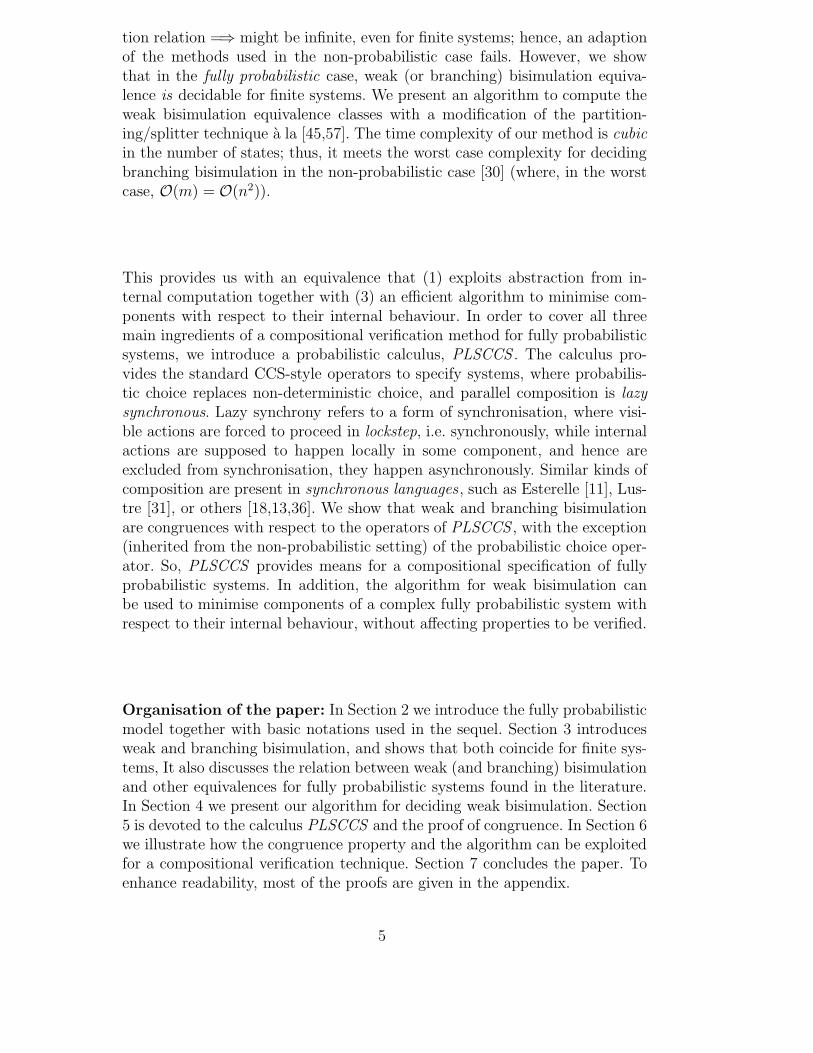
Fig. 3. s =ste s′ but s 6≈ s′

unique solution of the following linear equation system.

1. Q(s, L, α, C) = 0 if Prob(s, τ ∗α,C) = 0.2. If Prob(s, τ ∗α,C) > 0 then

Q(s, L, α, C) =P(s, α, C)

P(s, τ) + P(s, L)+∑u∈S

P(s, τ, u)

P(s, τ) + P(s, L)·Q(s, L, α, C).

Note that Prob(s, τ ∗α,C) > 0, α ∈ L implies P(s, τ) + P(s, L) > 0. If L ∈Offr∗ and α ∈ (Act \ τ)∗ then we put Q(s, L, α) = Q(s, L, α, S). Thisprobability Q(s, L, α) denotes the probability of performing the sequence α(interweaved with arbitrary many internal steps) from state s when offered astring of L. It is the basis of strong testing equivalence, =ste.

Definition 3.11 s =ste s′ iff for all L ∈ Offr ∗, α ∈ (Act \ τ)∗,

Q(s, L, α) = Q(s′, L, α)

Theorem 3.12 ≈ is strictly finer than =ste.

Proof: In Appendix A.2, Theorem A.20 we show that ≈ is finer than =ste.To see that =ste and ≈ do not coincide consider the fully probabilistic systemof Figure 3. Then, s =ste s

′ as, for instance,

Q(s, α, β, α) = 34

= 12

+ 12· 1

2= Q(s′, α, β, α)

and Q(s, α, α) = 1 = Q(s′, α, α). On the other hand,

Prob(s′, τ ∗α, S) = 3/4 > 1/2 = Prob(w′, τ ∗α, S).

Hence, s′ 6≈ w′. Thus, Prob(s′, τ ∗,W ) = 1/2 > 0 = Prob(s, τ ∗,W ) where W isthe weak bisimulation equivalence class of w′. Thus, s 6≈ s′.

Algorithms for deciding the three kinds of testing equivalences are presentedin [17]. They are based on iteratively solving linear equation systems, and runin time O(n4) where n is the number of states of the underlying system. Aswe will see in Section 4, using our (finer) notion of weak bisimulation insteadresults in a reduction of complexity, since our algorithm runs in cubic time.The reason is that our algorithm uses conditional probabilities which can

16

xw

u v

t

s

α, 1

β, 12

β, 12

γ, 1 β, 1

w′

u′

t′1

s′

t′2

v′

x′

α, 12

α, 12

β, 1

γ, 1

β, 1

β, 1

@@@R?

? ?

@@@R ? ?

? ?

Fig. 4. s ≡ s′ but s 6≈ s′

be computed by simple arithmetic operations rather than by solving linearequation systems.

Testing equivalences of Cleaveland et al: In [19] (see also [73]) quantitativeextensions of the non-probabilistic testing preorders by de Nicola&Hennessy[55,38] are discussed. Given a test T – which is represented by a fully prob-abilistic system equipped with a set of success states – the probability for afully probabilistic process P to pass the test T is defined as the probabilitymeasure of the set of ’interaction sequences’ leading to a success state. Intu-itively, given a class of tests, two fully probabilistic processes P, P ′ are testingequivalent with respect to a certain class of tests iff P and P ′ pass all tests Tof that class with the same probability. Two classes of tests are considered in[19]:

• the class Tests0 of τ -free tests which yields the testing equivalence ≡0,• the class Tests of all tests that do not contain ’τ -loops’ which yields the

testing equivalence ≡.

The exact definition (more precise, an alternative characterisation) of ≡0 isgiven in Appendix A.2 where we prove that ≡0 is coarser than ≈. For theprecise definition of ≡ see [19] or [73].

Theorem 3.13

(a) ≈ is strictly finer than ≡0.(b) ≈ and ≡ are incomparable.

Proof: In Appendix A.2, Theorem A.27 we show that ≈ is finer than ≡0.As pointed out in [73], the states s and s′ of the system shown in Figure 4are testing equivalent with respect to ≡ (and hence, testing equivalent withrespect to ≡0). On the other hand, s and s′ are not weakly bisimulationequivalent, because Prob(s, τ ∗ατ ∗, T ) = 1 while Prob(s′, τ ∗ατ ∗, T ) = 0 whereT denotes the weak bisimulation equivalence class of t. (Note that neither t′1nor t′2 is weakly bisimulation equivalent to t.) To illustrate that ≈ and ≡ areincomparable, we remark that the states s0 and s′0 of the system shown below

17

are weakly bisimulation equivalent, but s0 6≡ s′0.

s0 s′0 u τ , 1 α, 1

t

success u

τ , 1

2 α, 12

- -

@@@R

For instance, the test T shown on the right distinguishes the states s0 and s′0.The probability for s0 to pass the test T is 3/4 while the probability for s′0 topass T is 1/2.

4 Deciding weak bisimulation equivalence

In this section we develop an algorithm to compute the weak bisimulationequivalence classes. As pointed out earlier, an efficient algorithm for finitestate systems is crucial for mechanised verification purposes, since it allowsto minimise systems with respect to their internal behaviour. The generalidea of our algorithm is to use a partition refinement technique similar to theones proposed by Kanellakis&Smolka [45] resp. Paige&Tarjan [57] for decidingstrong bisimulation equivalence in the non-probabilistic case.

For a given finite set S of states, a partition X of S is a set C1, . . . , Cnsuch that

⋃i Ci = S and where the Ci are pairwise disjoint. The elements of a

partition X are sets of states, and are called blocks in the sequel. Each partitionX of S induces an equivalence relation

⋃C∈X C × C on S. Vice versa, the set

of equivalence classes of some equivalence relation on S form a partition of S.Therefore, in the sequel we blur the distinction between between a partitionand its induced equivalence, and between blocks and equivalence classes.

The general idea of partition refinement to compute weak bisimulation equiv-alence is as follows: The algorithm starts with some ’simple’ initial partitionXinit that is coarser than ≈ and then successively refines the given partition Xwith the help of a ’splitter’ of X , eventually resulting in the set of weak bisim-ulation equivalence classes. The crucial point is the definition of a splitter. Apossible candidate for a ’splitter’ of a partition X is a pair (a, C) ∈ Act × Xthat violates the condition for X to be a weak bisimulation, i.e.

(*) Prob(s, τ ∗aτ ∗, C) 6= Prob(s′, τ ∗aτ ∗, C) for some B ∈ X and s, s′ ∈ B.

One approach for a partition refinement algorithm would be to refine X ac-cording to a splitter in the sense of (*), i.e. to replace X by Refine ′(X , a, C) =B/ '(a,C): B ∈ X where

s '(a,C) s′ iff Prob(s, τ ∗aτ ∗, C) = Prob(s′, τ ∗aτ ∗, C).

18

The probabilities Prob(s, τ ∗aτ ∗, C) can be computed by solving the linearequation system (cf. [8]).

xs = 1 if a = τ and s ∈ Cxs = 0 if Path ful(s, τ

∗aτ ∗, C) = ∅xs =

∑t∈S

P(s, τ, t) · xt + P(s, a, C)

if Path ful(s, τ∗aτ ∗, C) 6= ∅ and a 6= τ ∨ s /∈ C.

The test whether Path ful(s, τ∗aτ ∗, C) = ∅ can be done by a reachability analy-

sis of the underlying directed graph, e.g. with a depth first search like method.Then, Ω(n3.8) is an asymptotic lower bound for the time complexity of thismethod, where, n is the number of states. Note that in the worst case weneed n refinement steps and in each refinement step we have to solve a linearequation system with n variables and n equations (which takes O(n2.8) timewith the method of [2]).

As a more efficient alternative, we develop an algorithm that runs in timeO(n3) in the sequel. The basic idea is to replace (*) by a condition that assertsthat X violates the conditions of a branching bisimulation. To realise this idea,we use an alternative definition of a splitter that is based on an characterisationof branching bisimulations which uses the conditional probability PX (s, a, C),the probability to reach a block C ∈ X from state s via action a within onestep under the condition that the system does not make an internal moveinside the block (of X ) that contains s. These conditional probabilities canbe computed by simple arithmetic operations. Thus, the use of this kind ofsplitters has the advantage that in the refinement steps we do not have tosolve linear equation systems.

4.1 The algorithm

In what follows, we fix a finite fully probabilistic system (S,Act ,P) and apartition X of S. [s]X denotes the unique block in X that contains s. We saythat X is a weak (branching) bisimulation iff the induced equivalence relationRX =

⋃C∈X C × C is a weak (branching) bisimulation. We use Sterm to

denote the set of terminal states (i.e. all states s ∈ S where P(s, a, t) = 0 forall a ∈ Act and t ∈ S). Furthermore,

Definition 4.1 We say that state s is silent, if s is terminal or P(s, τ, [s]X ) =1, otherwise we call state s non-silent. We let

SXns = s ∈ S \ Sterm : P(s, τ, [s]X ) < 1

denote the set of all non-silent states with respect to X .

19

Thus a non-silent states will with non-zero probability either perform some-thing visible (in case that P(s, τ) < 1) or silently step into a different class(in case that P(s, τ, t) > 0 for some t /∈ [s]X ).

Definition 4.2 If s ∈ SXns and (a, C) ∈ Act × X with (a, C) 6= (τ, [s]X ) thenwe define

PX (s, a, C) =P(s, a, C)

1−P(s, τ, [s]X ).

PX (s, a, C) is the conditional probability for non-silent state s to reach blockC via action a under the condition that being in state s the system doesnot make a silent move inside the block [s]X (i.e. it performs a visible actionor makes a τ -move to another block). With this conditional probability, weget the following alternative characterisation of branching bisimulations thatrefers to the probabilities PX (·) rather than the values ProbRX (·).

Lemma 4.3 X is a branching bisimulation iff, for all B ∈ X with B∩SXns 6= ∅:

(1) PX (s, a, C) = PX (s′, a, C)for all s, s′ ∈ B ∩ SXns and (a, C) ∈ Act ×X with (a, C) 6= (τ, B).

(2) If s0 ∈ B \ SXns then there exists a finite path σ with• first(σ) = s0,• σ(i) ∈ B \ SXns , i = 0, 1, . . . , |σ| − 1,• last(σ) ∈ B ∩ SXns .

Proof: see Appendix A.1, Lemma A.10.

This lemma says that a block B (containing non-silent states) of a branchingbisimulation consists of (1) all non-silent states exhibiting the same conditionalvalues PX (·, a, C), together with (2) those silent states that can silently evolveonly to non-silent states of the same block.

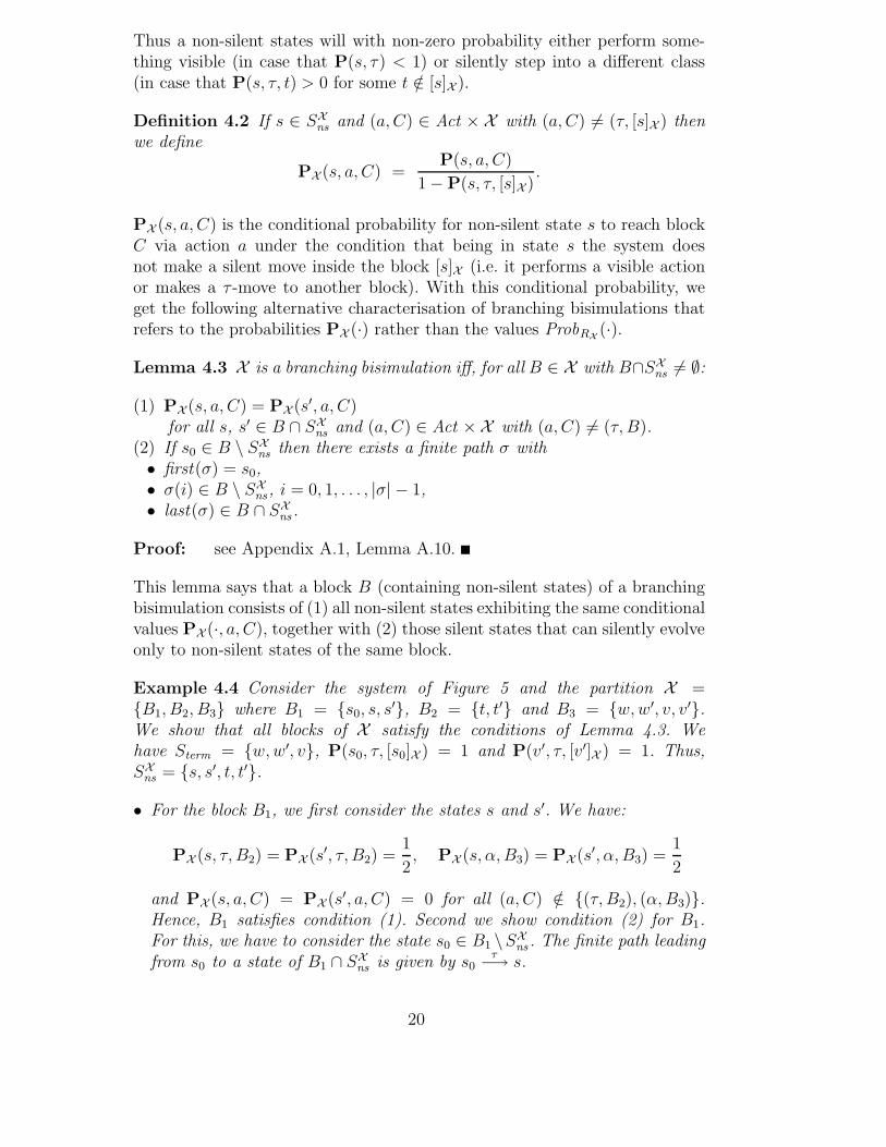
Example 4.4 Consider the system of Figure 5 and the partition X =B1, B2, B3 where B1 = s0, s, s

′, B2 = t, t′ and B3 = w,w′, v, v′.We show that all blocks of X satisfy the conditions of Lemma 4.3. Wehave Sterm = w,w′, v, P(s0, τ, [s0]X ) = 1 and P(v′, τ, [v′]X ) = 1. Thus,SXns = s, s′, t, t′.

• For the block B1, we first consider the states s and s′. We have:

PX (s, τ, B2) = PX (s′, τ, B2) =1

2, PX (s, α, B3) = PX (s′, α, B3) =

1

2

and PX (s, a, C) = PX (s′, a, C) = 0 for all (a, C) /∈ (τ, B2), (α,B3).Hence, B1 satisfies condition (1). Second we show condition (2) for B1.For this, we have to consider the state s0 ∈ B1 \SXns . The finite path leadingfrom s0 to a state of B1 ∩ SXns is given by s0

τ−→ s.

20

• For the block B2 = t, t′ we get: PX (t, β, B3) = PX (t′, β, B3) = 1 andPX (t, a, C) = PX (t′, a, C) = 0 for all (a, C) 6= (β,B3). Hence, B2 satisfies(1). As B2 ∩ SXns = ∅, B2 fulfills condition (2).

• As B3 ∩ SXns = ∅ for the block B3 there is nothing to show.

Lemma 4.3 yields that X is a branching bisimulation.

The lemma does not impose constraints on those classes of a branching bisim-ulation that consist of silent states only. So, let X be a branching bisimulationand B ∈ X such that B∩SXns = ∅. By the definition of silence, s ∈ B implies ei-ther that s is terminal or P(s, τ, B) = 1. In either case, ProbRX (s, τ ∗α,C) = 0and ProbRX (s, τ ∗, C) = 0 if C ∈ X is distinct from B. Having this in mind,we can show how the ProbRX (s, τ ∗a, C) can be derived from the conditionalprobabilities PX (t, a, C) if X is a branching bisimulation.

Lemma 4.5 If X is a branching bisimulation then for all B ∈ X , s ∈ Bimplies

• ProbRX (s, τ ∗, C) = PX (B, τ, C) for all C ∈ X ,• ProbRX (s, τ ∗α,C) = PX (B, α, C) for all α ∈ Act \ τ and C ∈ X , where

PX (B, a, C) =

PX (t, a, C) : if (a, C) 6= (τ, B), B ∩ SXns 6= ∅, and t ∈ B ∩ SXns

0 : if (a, C) 6= (τ, B) and B ∩ SXns = ∅

1 : if (a, C) = (τ, B).

Proof: see Appendix A.1, Lemma A.11.

Since by Lemma 4.3 each non-silent state s in class B exhibits the same

PX (s, a, C) =P(s, a, C)

1−P(s, a, C)

value, the definition of PX (B, a, C) is well-defined. It seems worth to pointout that the above fraction may not return the same values if (a, C) = (τ, B).In other words, if X is a branching bisimulation, B ∈ X and s, s′ ∈ B ∩ SXns

thenP(s, τ, B)

1−P(s, τ, B)6= P(s′, τ, B)

1−P(s′, τ, B)

is possible. For instance, for the states s and s′ in Example 4.4 (Figure 5)we have s ≈br s′ but P(s, τ, B1)/(1− P(s, τ, B1)) = 0 while P(s′, τ, B1)/(1−P(s′, τ, B1)) = 1/2 (where B1 = s0, s, s

′ is the branching bisimulation equiv-alence class of s and s′).

As indicated above, the algorithm to compute branching (and hence weak)bisimulation equivalence is based on the values of PX to refine partitions by

21

w

t v

s

s0

τ , 1

τ , 12

α, 12

β, 1

t′

w′

s′

v′

τ , 13 α, 1

3

τ , 13

τ , 1β, 1

@@@R

?

?

?

@@@R

Fig. 5. Branching bisimulation equivalent fully probabilistic systems

means of splitters:

Definition 4.6 A splitter of a partition X is a tuple (a, C) consisting of anaction a ∈ Act and some C ∈ X such that there exists some B ∈ X with(τ, B) 6= (a, C) and PX (s, a, C) 6= PX (s′, a, C) for some states s, s′ ∈ B∩SXns .

The main idea for refining a given partition X via a splitter (a, C) is to isolatein each B ∈ X with (τ, B) 6= (a, C) those states non-silent states s, s′ ∈ Bwhere PX (s, a, C) = PX (s′, a, C), in order to ensure condition (1) of Lemma4.3. By condition (2) of the lemma, each such equivalence class A of B ∩SXns has to be enriched with exactly those silent states states of B that canreach A via internal actions and that cannot reach any other equivalence classA′ of B ∩ SXns without passing A. So, we define the splitting of a block Bby means of a splitter (a, C) for the non-silent members of B first. This isperformed by means of a function NonSilentSplit(B, a, C), that only groupsnon-silent states. Silent states are treated afterwards, by means of a silenceclosure operation. In short, if A is a class of equivalent non-silent states in Bthen SilenceClose(A,B) enriches A by all silent states of B for which all finitepaths of internal steps that end up in a non-silent state actually end up in A.

Definition 4.7 Let (a, C) be a splitter of a partition X and B ∈ X such that(τ, B) 6= (a, C). We define

NonSilentSplit(B, a, C) = (B ∩ SXns)/ ≡X

where, for s, s′ ∈ B ∩ SXns , s ≡X s′ iff PX (s, a, C) = PX (s′, a, C).

Furthermore, if A ∈ NonSilentSplit(B, a, C) then we define the silence closureSilenceClose(A,B) of A to be the largest subset A of B which contains A andsuch that for all s ∈ A \ A:

• P(s, τ, A) = 1• There exists a finite path σ with· first(σ) = s,· σ(i) ∈ A \ A, i = 0, 1, . . . , |σ| − 1,· last(σ) ∈ A.

22

The residuum of B with respect to (a, C) is given by

Res(B, a, C) = B \B′ \ ∅ where B′ =⋃

A∈NonSilentSplit(B,a,C)

SilenceClose(A,B).

The residuum contains a singleton set of all silent states that are not coveredby any silence closure SilenceClose(A,B) if there are such states. Otherwise,the residuum is an empty set. The states contained in this singleton set pos-sess non-zero probability of silently evolving to distinct, non-equivalent statesinside B, Therefore, they do not belong to a particular silence closure, andhence have to be separated. The refinement operator Refine of a partition bymeans of a splitter is now easy to define as a collection of the sets we havedefined above.

Definition 4.8 Let X be a partition, (a, C) a splitter of X . For B ∈ X , wedefine:

• If (a, C) = (τ, B) then Refine(B, a, C) = B.• If (a, C) 6= (τ, B) then

Refine(B, a, C) = SilenceClose(A,B) : A ∈ NonSilentSplit(B, a, C)

∪ Res(B, a, C).

We define Refine(X , a, C) =⋃B∈X Refine(B, a, C).

Clearly, for each partition X which is coarser than S/ ≈br and each splitter(a, C) of X , the partition Refine(X , a, C) is coarser than S/ ≈br and strictlyfiner than X . Our refinement operator preserves condition (2) of Lemma 4.3.More precisely, if B ∈ X such that B∩SXns = ∅ and condition (2) of Lemma 4.3is fulfilled then all blocks A ∈ Refine(B, a, C) fulfill condition (2). Moreover,if X is a partition that is coarser than S/ ≈br , and fulfills condition (2)of Lemma 4.3, and there does not exist a splitter for X then X = S/ ≈br.Hence, X contains the weak bisimulation equivalence classes (by Theorem 3.9).These observations lead to the following algorithm. We start with a ’simple’partition X that satisfies condition (2) of Lemma 4.3 and that is coarser than≈. Then we apply the refinement operator to X , as long as X can be refined,i.e. as long as there exists a splitter for X , eventually resulting in the partitionX = S/ ≈.

Since the initial partition has to fulfill condition (2) of Lemma 4.3 the ini-tialisation of the algorithm requires care. We cannot start with the ’trivial’partition X = S (that identifies all states) as it might actually violate con-dition (2). For instance, for a system with two states, a terminal state t anda state s with P(s, α, t) = 1, the trivial partition Xtrivial = s, t does nothave a splitter. Hence, if we would start with Xtrivial then our algorithm would

23

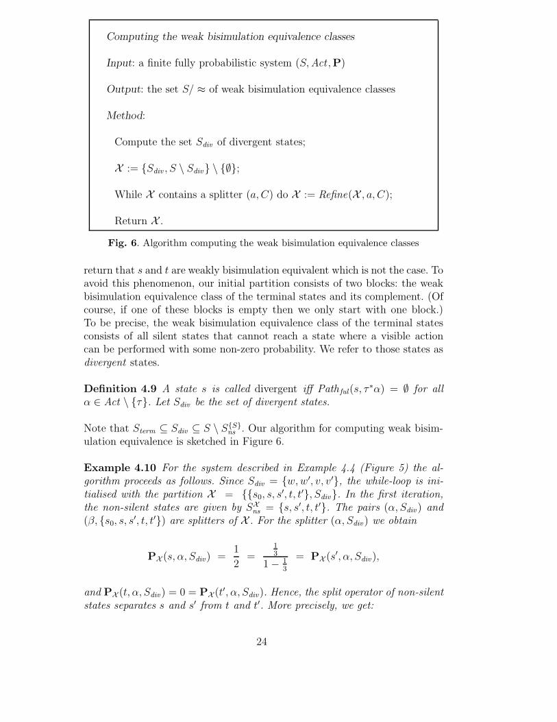
Computing the weak bisimulation equivalence classes

Input: a finite fully probabilistic system (S,Act ,P)

Output: the set S/ ≈ of weak bisimulation equivalence classes

Method:

Compute the set Sdiv of divergent states;

X := Sdiv , S \ Sdiv \ ∅;

While X contains a splitter (a, C) do X := Refine(X , a, C);

Return X .

Fig. 6. Algorithm computing the weak bisimulation equivalence classes

return that s and t are weakly bisimulation equivalent which is not the case. Toavoid this phenomenon, our initial partition consists of two blocks: the weakbisimulation equivalence class of the terminal states and its complement. (Ofcourse, if one of these blocks is empty then we only start with one block.)To be precise, the weak bisimulation equivalence class of the terminal statesconsists of all silent states that cannot reach a state where a visible actioncan be performed with some non-zero probability. We refer to those states asdivergent states.

Definition 4.9 A state s is called divergent iff Path ful(s, τ∗α) = ∅ for all

α ∈ Act \ τ. Let Sdiv be the set of divergent states.

Note that Sterm ⊆ Sdiv ⊆ S \ SSns . Our algorithm for computing weak bisim-ulation equivalence is sketched in Figure 6.

Example 4.10 For the system described in Example 4.4 (Figure 5) the al-gorithm proceeds as follows. Since Sdiv = w,w′, v, v′, the while-loop is ini-tialised with the partition X = s0, s, s

′, t, t′, Sdiv. In the first iteration,the non-silent states are given by SXns = s, s′, t, t′. The pairs (α, Sdiv) and(β, s0, s, s

′, t, t′) are splitters of X . For the splitter (α, Sdiv) we obtain

PX (s, α, Sdiv) =1

2=

13

1− 13

= PX (s′, α, Sdiv),

and PX (t, α, Sdiv) = 0 = PX (t′, α, Sdiv). Hence, the split operator of non-silentstates separates s and s′ from t and t′. More precisely, we get:

24

NonSilentSplit(s0, s, s′, t, t′, α, Sdiv) = s, s′, t, t′,

NonSilentSplit(Sdiv , α, Sdiv) = ∅.

The silence closure operator yields

SilenceClose(s, s′, s0, s, s′, t, t′) = s0, s, s

′,SilenceClose(t, t′, s0, s, s

′, t, t′) = t, t′,SilenceClose(∅, Sdiv) = ∅,

and Res(Sdiv , α, Sdiv) = Sdiv . Hence, we get the partition

X := Refine(X , α, Sdiv) = s0, s, s′, t, t′, w,w′, v, v′

as a result of the first iteration of the loop. No further splitter exists for thispartition. So, our algorithm returns X containing the weak bisimulation equiv-alence classes.

4.2 Complexity of the algorithm

In order to establish the time and space complexity of the algorithm, we letn = |S|. We suppose that the alphabet Act is fixed, i.e. we treat the size |Act |as a constant.

Theorem 4.11 The algorithm of Figure 6 can be implemented in time O(n3)and space O(n2).

Proof: The initialisation of the algorithm has quadratic time (and space)complexity, since Sdiv can be computed by a reachability analysis in the un-derlying directed graph. We compute all states that can reach a state oft ∈ S : P(t, α) > 0 for some α ∈ Act \ τ, e.g. by a standard depth firstsearch. Then, the computation of the initial partition X needs O(n2) timeand space. To establish a complexity result for the complete algorithm re-quires more details concerning the implementation of a refinement step. Eachrefinement step consists of two phases, a preparatory phase and a splittingphase, where refinement, i.e. splitting of blocks, actually takes place.

Preparatory phase: Let X be the current partition. We compute the valuesP(s, a, C) and PX (s, a, C) for each s ∈ S, a ∈ Act and C ∈ X . The set SXns

can be derived from the probabilities PX (s, τ, C), s ∈ C. For each pair (a, C)(where a ∈ Act and C ∈ X ) and A ∈ X we compute

min(A, a, C) = mins∈A

PX (s, a, C), max(A, a, C) = maxs∈A

PX (s, a, C).

25

Then, (a, C) is a splitter of X iff min(A, a, C) < max (A, a, C) for some Awith (a, C) 6= (τ, A). If there is no splitter of X then X = S/ ≈. Otherwisewe choose some splitter (a, C) of X .

Splitting phase: For all B ∈ X with (τ, B) 6= (a, C) we compute the setRefine(B, a, C) as follows. We construct an ordered binary tree Tree(B) bysuccessively inserting the values PX (s, a, C), s ∈ B ∩ SXns . Each node v ofTree(B) is represented as a record with components v.key and v.states . Foreach state s ∈ B ∩ SXns , we traverse the tree Tree(B) starting in the root andwe search for the value PX (s, a, C).

• If we reach a node v with v.key = PX (s, a, C) then we insert s into v.states .• Otherwise, PX (s, a, C) is not yet represented in Tree(B) and we insert a

node v with v.key = PX (s, a, C) and v.states = s.

In the final tree, v.states is the set of states s ∈ B ∩ SXns with PX (s, a, C) =v.key . Thus, the nodes of the final tree Tree(B) represent the sets A ∈NonSilentSplit(B, a, C). More precisely,

NonSilentSplit(B, a, C) = v.states : v is a node in Tree(B).

We derive Refine(B, a, C) by means of a topological sorting of silent states inB. Let GB be the directed graph (B,EB) where (s, t) ∈ EB iff P(t, τ, s) > 0and t ∈ B \SXns (note that edges are ’reversed’ in this graph). We compute thesets SilenceClose(A,B), A ∈ NonSilentSplit(B, a, C), by the following breadthfirst search like method. We use three kinds of labels for the states:

• label(s) = ⊥ iff s ∈ B \ SXns and s is not yet visited.• label(s) = A ∈ NonSilentSplit(B, a, C) iff s is reachable in GB from some

state in A but there is no other A′ ∈ NonSilentSplit(B, a, C) where a pathfrom a state of A′ to s in GB is already detected.• label(s) = ∗ iff there are two sets A, A′ ∈ NonSilentSplit(B, a, C) such thats is reachable from a state in A and from a state in A′. (In particular, allsuccessors of a ∗-labelled state in GB are also labelled by ∗.)

Initially, we define label(s) = ⊥ for all s ∈ B \ SXns and label(s) = A for alls ∈ A and A ∈ NonSilentSplit(B, a, C). (The implementation might use therespective v.key values computed before as identifiers (labels) for different A).

We use a queue Q which initially contains the states s ∈ A, A ∈NonSilentSplit(B, a, C). While Q is not empty we take the first element sof Q, remove s from Q and, if label(s) 6= ∗ then, for all t ∈ B \ SXns with(s, t) ∈ EB, we do:

(1) If label(t) = ⊥ then we add t to Q and set label(t) = label(s).(2) If label(t) ∈ NonSilentSplit(B, a, C), label(t) 6= label(s), then we set

26

label(u) = ∗ for u = t and all successors u of t in GB. 1

Then, SilenceClose(A,B) = s ∈ B : label(s) = A, Res(B, a, C) = s ∈ B :label(s) ∈ ⊥, ∗ \ ∅.

Complexity: It is clear that the method described above can be implementedin space O(n2). We show that the time complexity of our method is O(n3).First, we observe that there are at most n iterations of the refinement step.Thus, it suffices to show that each refinement step takes time O(n2).

First we observe that for each iteration (i.e. each refinement step), thepreparatory phase requires O(n2) time, 2 in order to compute the valuesP(s, a, C), and to decide whether a splitter exist. If so, the splitting phaseis entered, where the trees Tree(B) are subsequently constructed. Rangingover all B, the construction of the trees, and hence the computation of thesets NonSilentSplit(B, a, C) takes O(n log n) time if one resorts to some kindof ordered balanced trees. We show that, ranging over all B ∈ X , the setsSilenceClose(·, B) and Res(B, a, C) can be derived in time O(n2): For fixedB ∈ X , the directed graph GB can be constructed in time O(|B|2). Each states ∈ B is added to Q at most once. (Note that only states with label ⊥ can beadded to Q.) Each state t which is visited by a depth first search in step (2) islabelled by ∗. Thus, it can never be visited in step (2) once again. As a conse-quence, each state causes time costs (at most) of order 2n in the computationof Refine(B, a, C): as an element of Q and as a state with label 6= ∗ that isvisited in step (2). Either case involves O(n) computations. Summing up overall s ∈ B, the computation of Refine(B, a, C) has time complexity O(|B| · n).So, we obtain Refine(X , a, C) in time O(n2).

5 Lazy synchronous CCS

Process calculi such as Milner’s CCS or SCCS [51–53], Hoare’s CSP [39],Bergstra&Klop’s ACP [10] or the ISO standard LOTOS [40] are importanthigh-level specification means for compositional design and analysis of par-allel systems. Such process calculi are usually equipped with an interleavingsemantics, where (apart from synchronous calculi) the concurrent executionof independent actions is modelled by interleaving the actions in all possibleorders. Nondeterminism is used to describe the freedom in the choice which

1 This may be realised by a depth first search starting in t to find all successors oft. States that are already labelled by ∗ are ignored.2 Note that for each tuple (s, a, C) we have to calculate

∑t∈C P(s, a, t). Hence, for

fixed a and ranging over all s ∈ S, C ∈ X , we get the time complexity O(n2). Sincewe suppose Act to be fixed, the values P(s, a, C) can be computed in time O(n2).

27

independent action is executed next.

During the last decade, these calculi have been extended in several ways inorder to provide means to specify the probabilistic behaviour of parallel sys-tems within the same formalism [32,50,54,37,35,3]. The essential ingredient isthe incorporation of a probabilistic choice operator. Distinguishing fine pointsin this variety of approaches are (1) the interplay of probabilistic choice withnondeterministic choice, and (2) the semantics of parallel composition. 3

In the fully probabilistic setting considered in this paper, nondeterminism iscompletely ruled out. So, addressing the first of the above two issues, proba-bilistic choice replaces nondeterministic choice, instead of letting both choiceoperators coexist. The second issue, semantics of parallel composition has re-ceived considerable attention in the fully probabilistic setting [23]. Due to theabsence of nondeterminism, the model is not closed under the usual nondeter-ministic interleaving of all independent actions.

Instead, we introduce in the sequel a new, lazy synchronous parallel compo-sition operator. Before we explain lazy synchronous parallel composition, webriefly review two other main strands followed in the definition of fully prob-abilistic parallel composition. One approach replaces nondeterministic inter-leaving by probabilistically scheduled interleaving [5,67,56,66,29]. For this pur-pose, the parallel composition operator is decorated with a set of parameters.These parameters are used to quantify the probability of each nondetermin-istic alternative that arises in a parallel composition. In this way, the fullyprobabilistic model remains closed under parallel composition, but an intu-itive interpretation of the parameters involved is often difficult. [23] containsa classification of these approaches, and defines criteria to be fulfilled by anappropriate probabilistically scheduled parallel composition.

The other major approach, synchronous parallelism, has been proposed by[25,27]. Synchrony refers to a drastically different view on the evolution ofprocesses. Instead of assuming that actions may occur independently and con-currently, synchrony means that all parallel components have to interact (orexplicitly signal that they intend to idle) in each time step, they proceed inlockstep [52]. In this way one avoids to make a scheduling decision since allcomponents must perform a step. Several approaches that have appeared inthe literature [25,43,68,49,70,27,47] deal with the synchronous product P1×P2

in the style of Milner’s SCCS where each step of P1 × P2 is composed by ex-actly one action of P1 and P2. The probability of such a step is determinedby the product of the individual probabilities of each action involved.

3 A third, less obvious, distinguishing feature lies in the semantics of probabilisticchoice, where the probabilistic decision of the process may either be conditionalon the actions offered by the environment (external probabilistic choice) or totallyindependent of what is offered (internal probabilistic choice) [50,54].

28

P ::= nil∣∣∣ Z ∣∣∣ a.P ∣∣∣ ⊕i∈I [pi]Pi

∣∣∣ P1 ⊗ P2

∣∣∣ P \ L∣∣∣ P[`]

Fig. 7. Syntax of PLSCCS expressions

We deviate from these approaches and introduce a form of synchrony that isless rigid. In fact, our concept of lazy synchrony has been used in the proba-bilistic setting by other authors (e.g. [24,36]) as well. In these approaches, theprocesses P1 and P2 have to synchronise at certain synchronisation points butperform sequences of independent actions in isolation between these synchro-nisation points. In the non-probabilistic setting, similar kinds of compositionare present in synchronous languages, such as Esterelle [11], Lustre [31], orothers [18,13,36]. In what follows, we build upon this intuition, and define alazy synchronous probabilistic variant of CCS, denoted PLSCCS , where vis-ible actions are forced to proceed in lockstep, while internal actions τ areexecuted independently. We show that weak (as well as strong) bisimulationis a congruence for the operators of PLSCCS (except for a rather standarddeficiency with respect to choice).

5.1 PLSCCS : a lazy synchronous calculus

In PLSCCS , internal actions are executed independently, while visible actionsare forced to proceed in lockstep. In other words, each step of the lazy productP1 ⊗ P2 is composed by sequences of steps of P1 and P2, where each of themstarts with an arbitrary number of internal transitions (labelled τ) and endsup with a visible action α. (Recall our convention to use greek letters forvisible actions only.) Hence, the probabilities for the transitions of P1⊗P2 aregiven by the product of the individual probabilities where we deal with thecumulative effect of τ -transitions. Syntax and semantics of all other operatorsare similar to SCCS; apart from the probabilistic choice operator⊕i∈I [pi]Pi,replacing the nondeterministic choice

∑i∈I Pi of SCCS.

Syntax of PLSCCS : Let Var be a set of process variables. PLSCCS ex-pressions are given by the grammar shown in Figure 7. Here, Z ∈ Var ,a ∈ Act , L ⊆ Act , I is a countable indexing set, pi are real numbers pi ∈ ]0, 1]with

∑pi = 1 and ` : Act −→ Act is a relabelling function with `(τ) = τ .

PLSCCS denotes the collection of all PLSCCS expressions. For finite indexingset I = i1, . . . , in, we also write [pi1 ]Pi1⊕ . . .⊕ [pin ]Pin instead of⊕i∈I [pi]Pi.

As it is common practice in process calculi, we will use process equations of

the form Zjdef= Pj, j = 1, . . . , k, to specify recursive behaviour. In the

above equations, Z1, . . . , Zk are pairwise distinct process variables (taken from

29

Var), and P1, . . . ,Pk are expressions given by the above grammar. They mayitself contain process variables. Technically, process equations are denoted bymeans of a function ∆ that assign to each process variable Z an expression∆(Z) (i.e. ∆ : Var −→ PLSCCS). A PLSCCS process is a pair P = 〈∆,P〉consisting of a declaration ∆ and an expression P. The intended meaning ofa process P = 〈∆,P〉 is that the behaviour of P is given by the expression Pwhere each occurrence of a process variable Z in P is viewed as a recursivecall of expression ∆(Z). If op is a n-ary operator symbol of the calculus andPi = 〈∆,Pi〉, i = 1, . . . , n, are processes then we write op(P1, . . . ,Pn) asshorthand for the process 〈∆, op(P1, . . . ,Pn)〉. PLSCCS denotes the set of allPLSCCS processes, i.e. pairs P = 〈∆,P〉 consisting of a declaration ∆ and anexpression P ∈ PLSCCS.

Example 5.1 The expressions

P = τ.( [1/2] τ.β.nil⊕ [1/2] α.nil ),

P′ = [1/3] τ.Z ⊕ [1/3] τ.β.nil⊕ [1/3] α.Y , and

P′′ = τ.Y.

are elements of PLSCCS. For a declaration ∆′ such that ∆′(Z) = P′ and∆′(Y ) = P′′, 〈∆′,P′〉 is a PLSCCS process.

The intended meanings of inaction nil, prefixing a.P, restriction P \ L andrelabelling P[`] are as in the case of standard (S)CCS. The probabilistic choiceoperator ⊕i∈I [pi]Pi is internal: if Pi, i ∈ I, are pairwise distinct then, withprobability pi, ⊕i∈I [pi]Pi behaves as Pi, independent of what is offered bythe environment.

As already mentioned, P1⊗P2 represents the lazy product of P1 and P2. Since⊗ treats τ as a local action and only synchronises visible actions, we assumea function

(Act \ τ)× (Act \ τ) −→ Act , (α, β) 7→ α ? β.

where, α ? β stands for the result of the synchronisation on the visible ac-tions α and β. Note that visible actions have to synchronise, but may becomeinvisible in doing so, because α ? β = τ is possible. Each a-labelled transi-tion of the lazy product P1 ⊗ P2 is then composed by sequences of steps ofthe components P1 and P2 that are labelled by strings of the form τ ∗α andτ ∗β respectively such that a is the result of the synchronised execution of thevisible actions α and β (i.e. a = α ? β). In other words, the probability ofP1⊗P2 to move via the action a to P′1⊗P′2 is cumulated from all probabilitiesProb∆(P1, τ

∗α,P′1) · Prob∆(P2, τ∗β,P′2) where (α, β) ranges over all pairs of

visible actions satisfying that α ? β = a. Here, Prob∆(P, τ ∗α,P′) is the prob-ability for P to perform a sequence of internal actions followed by α ending

30

P∆(a.P, a,P) = 1

P∆(⊕i∈I [pi]Pi, a,P

′)

=∑i∈I

pi ·P∆(Pi, a,P′)

W∆(P, α,P′) = P∆(P, α,P′) +∑

P′′∈PLSCCSP∆(P, τ,P′′) ·W∆(P′′, α,P′)

P∆(P1 ⊗ P2, a,P′1 ⊗ P′2) =

∑β?γ = a

W∆(P1, β,P′1) ·W∆(P2, γ,P

′2)

P∆(P \ L, a,P′ \ L) = P∆(P, a,P′) if a /∈ L

P∆(P[`], a,P′[`]) =∑

b∈`−1(a)P∆(P, b,P′)

P∆(Z, a,P′) = P∆(∆(Z), a,P′)

Fig. 8. Equations for P∆ and W∆ for the semantics of PLSCCS .

up in the state P′, with Prob∆ denoting the probability measure obtained bydeclaration ∆.

Operational semantics for PLSCCS : We supply PLSCCS with an oper-ational semantics with the help of a higher-order operator on function pairsthe form 〈P∆,W∆〉. The first function, P∆, in these pairs is an element of thefunction space PLSCCS×Act×PLSCCS −→ [0, 1], while the second one, W∆,is from PLSCCS× (Act \τ)×PLSCCS −→ [0, 1]. In the definition of the lazyproduct, W∆ is used to cumulate the probability of moving with a trace τ ∗αfrom P to P′, while P∆ represents the actual one-step transition probabilities.Formally,

Definition 5.2 For a fixed declaration ∆ : Var −→ PLSCCS, the semanticsof PLSCCS is defined as the fully probabilistic system (PLSCCS,Act ,P∆) wherethe transition probability function

P∆ : PLSCCS× Act × PLSCCS −→ [0, 1]

is given by the least function pair 〈P∆,W∆〉 satisfying the equations of Figure8.

The existence of a least function pair satisfying these equations can be derivedwith standard methods of domain theory, see e.g. [1].

Example 5.3 For the expressions P, P′, and P′′ of Example 5.1, and dec-laration ∆′ of Example 5.1, the operational semantics of P = 〈∆′,P〉 andP ′ = 〈∆′,P′〉 are depicted in Figure 9 (represented as trees, and where someintermediate states are not labelled.). The reader is invited to compare this

31

nil

nil

P

τ , 1

τ , 12

α, 12

β, 1 nil

P′

P′′

τ , 13 α, 1

3

τ , 13

τ , 1β, 1

@@@R

?

?

?

@@@R

Fig. 9. Operational semantics of P = 〈∆′,P〉 and P ′ = 〈∆′,P′〉.

nil⊗ nil nil⊗ nil nil⊗ P′′ nil⊗ P′′

P⊗ P′

β, 1

4α, 1

4τ , 1

4τ , 1

4

+

QQQQQQQs

AAAAAU

Fig. 10. Operational semantics of P ⊗ P ′.figure with Figure 5.

To illustrate the lazy product, Figure 10 contains the operational semantics ofP ⊗ P ′, where we assume a synchronisation function ?, such that α ? α = α,β ? β = β, and α ? β = β ? α = τ . For instance, the operational semanticsdefines P∆(P⊕ P′, τ, nil⊕ P′′) = 1/4 as a result of

P∆(P⊕ P′, τ, nil⊕ P′′) =∑

β?γ = τ

W∆(P, β, nil) ·W∆(P′, γ,P′′)

= W∆(P, β, nil) ·W∆(P′, α,P′′) +

W∆(P, α, nil) ·W∆(P′, β,P′′).

Obviously, W∆(P′, β,P′′) = 0 (since action β does not occur on any path fromP′ to P ′′), and hence only first summand might contribute non-zero probability.We calculate

W∆(P′, α,P′′) = P∆(P′, α,P′′) +∑

P′′′∈PLSCCS

P∆(P, τ,P′′′) ·W∆(P′′′, α,P′′)

=1

3+ P∆(P, τ,P) ·W∆(P′, α,P′′)

=1

3+

1

3·W∆(P′, α,P′′),

whose (least) solution is 1/2. Furthermore, we obtain W∆(P, β, nil) = 1/2,

32

nil

P

nil

P′

nil

P′′

a, 1

4 a, 13 a, 1

2

? ? ?

Fig. 11. Three sub-stochastic processes

and hence P∆(P⊕ P′, τ, nil⊕ P′′) = 1/4.

Our transition probability function is potentially sub-stochastic in the sensethat

∑a,t P∆(s, a, t) might be strictly between 0 and 1 (violating Definition

2.1). We identify any sub-stochastic probabilistic system (S,Act ,P) with thefully probabilistic system (S∪†Act∪†,P†) obtained by identifying P† withP on S ×Act × S, by setting

P†(s, †, †) = 1 −∑

a∈Act ,t∈SP(s, a, t),

and P†(·) = 0 in all remaining cases. The distinguished state † is a means torepresent a deadlock in the system. So, a state s in a sub-stochastic systemmay possess the potential of deadlocking with a certain probability, say p.In this case, P†(s, †, †) = p. Remark that, by definition, state † can only bereached via action †, and no other state can be reached via action †.

In the context of PLSCCS , sub-stochasticity can arise as a result of restriction,unguarded probabilistic choice, and recursion.

Example 5.4 For a declaration ∆ with ∆(Z) = Z, Figure 11 presents threesub-stochastic probabilistic systems obtained via the operational semantics forthe processes

P = ([1/4] a.nil⊕ [3/4] b.nil) \ a,

P′ = [1/3] a.nil⊕ [2/3] nil, and

P′′ = [1/2] a.nil⊕ [1/2]Z.

Accordingly, we obtain the deadlock probabilities

P†∆(P, †, †) =

3

4, P†

∆(P′, †, †) =2

3, and P†

∆(P′′, †, †) =1

2.

As far as we know, the use of fixed-point equations is novel when definingan operational semantics. We have chosen this style of definition, because thedefining equations as such are easy to understand, and the domain-theoreticarguments are not much involved. Alternatively, the semantics could be givenin terms of an (indexed) probabilistic transition relation using standard opera-tional rules, as it is done, for instance, for synchronous probabilistic CCS [25].

33

Lemma 5.5 For all P, P′ ∈ PLSCCS and α ∈ Act,

W∆(P, α,P′) = Prob∆(P, τ ∗α,P′).

Proof: easy verification. Uses structural induction on the syntax of P, andthe fact that Prob∆(P, τ ∗α,P′) is the least solution of the equation

Prob∆(P, α,P′) = P∆(P, α,P′) +∑

P′′∈PLSCCS

P∆(P, τ,P′′) · Prob∆(P′′, α,P′)

in the interval [0, 1].

So, W∆(P, τ ∗α,P′) determines the probability for the process 〈∆,P〉 to behaveas 〈∆,P′〉 after performing a sequence of τ -steps followed by visible action α.As exemplified in Example 5.3, the calculation of this probability boils downto the solution of a linear equation system (similar to the one appearing inSection 4 to compute Prob(s, τ ∗aτ ∗, C)), as long as we are dealing with a finiteprocess, i.e. where the operational semantics maps on a fully probabilisticprocess that is finite (or can be identified with a finite process).

Corollary 5.6 For all P1, P2, P′1, P′2 ∈ PLSCCS and a ∈ Act,

P∆(P1 ⊗ P2, a,P′1 ⊗ P′2) =

∑β?γ=a

Prob∆(P1, τ∗β,P′1) · Prob∆(P2, τ

∗γ,P′2).

Proof: Follows immediately from Lemma 5.5.

Comparison to synchronous probabilistic CCS: To facilitate the inspec-tion of the semantics, we highlight the distinguishing features of PLSCCS ,compared to the well-studied fully probabilistic variant of synchronous CCS[25,27], called PSCCS in the sequel.

• The internal action τ does not play any specific role in PSCCS . In particular,(Act, ?) is supposed to form an Abelian monoid, where τ is treated as anyother action.• The product P1×P2 of PSCCS is strictly synchronous. In terms of a higher

order operator, this semantics is obtained by replacing the equation forP1 ⊗ P2 in Figure 8 by

P∆(P1 × P2, a,P′1 × P′2) =

∑b?c = a

P∆(P1, b,P′1) ·P∆(P2, c,P2).

Then, the use of W∆ is superfluous.• Probabilistic choice in PLSCCS is internal, while it is external in PSCCS .

Since, in the (S)CCS context, the influence of the environment is madeexplicit by means of restriction, this implies that the semantics of restriction

34

differs between PSCCS and PLSCCS . PSCCS restriction (denoted PdL)involves renormalisation, and relies on the equation

P∆(PdL, a,P′dL) =P∆(P, a,P′)∑

b∈L,P′∈PLSCCSP∆(P, b,P′)

if a /∈ L.

In contrast, PLSCCS restriction P \L may induce nonzero deadlock proba-bilities, in case that an action is randomly chosen that is not offered by theenvironment.

5.2 Compositionality

In this section, we establish the congruence result (Theorem 5.8) statingthe compositionality of weak bisimulation with respect to the operators ofPLSCCS . More precisely, we show that weak bisimulation equivalence ≈ is acongruence with respect to the PLSCCS operators action prefixing, restriction,relabelling, lazy product and guarded probabilistic choice. In what follows, weshrink our attention to finite PLSCCS processes.

Definition 5.7 A PLSCCS process P = 〈∆,P〉 is called finite iff thereare only finitely many expressions P′ ∈ PLSCCS that are reachable from Pin (PLSCCS,Act ,P∆) with nonzero probability. A declaration ∆ : Var −→PLSCCS is called finite iff, for each Z ∈ Var, 〈∆, Z〉 is finite.

If 〈∆,P〉 is finite then (PLSCCS,Act ,P∆) can be identified with the finitefully probabilistic process that arises by removing all expressions that are notreachable from the initial state P. Obviously, if ∆ is finite then 〈∆,P〉 is,for arbitrary expressions P. A sufficient condition which guarantees that ∆ isfinite is ’regularity’ of ∆ in the sense that, for all process variables Z there isno occurrence of Z ′ in ∆(Z) that is contained in a subexpression of the formP[`], P \ L or P1 ⊗ P2.

To establish compositionality, we adapt weak bisimulation equivalence ≈ (andstrong bisimulation equivalence ∼) to PLSCCS processes as follows. Forfixed declaration ∆, we define the relations ≈∆ by P ≈∆ P′ iff P ≈ P′

holds in (PLSCCS,Act ,P∆). Similarly, we define P ∼∆ P′ iff P ∼ P′ in(PLSCCS,Act ,P∆), to lift strong bisimulation equivalence ∼. 4

Theorem 5.8 Weak bisimulation equivalence is preserved by the PLSCCS

4 Remark that in order to compare 〈∆′,P〉 and 〈∆′′,P′〉, where both ∆′ and ∆′′

are finite, but distinct, we may always use α-conversion to join ∆′ and ∆′′ to someequipotent declaration ∆α and expressions P′α and P′′α such that 〈∆′,P〉 and 〈∆α,P

′α〉

(as well as 〈∆′′,P′〉 and 〈∆α,P′′α〉) coincide.

35

operators action prefixing, restriction, relabelling and lazy product. More pre-cisely, if ∆ is a finite declaration, then for all PLSCCS expressions s, s′, Pi,P′i:

(a) If P ≈∆ P′ then a.P ≈∆ a.P′, P \ L ≈∆ P′ \ L, and P[`] ≈∆ P′[`].(b) If Pi ≈∆ P′i, i = 1, 2, then P1 ⊗ P2 ∼∆ P′1 ⊗ P′2; and thus,

P1 ⊗ P2 ≈∆ P′1 ⊗ P′2.

(c) Weak bisimulation equivalence is a congruence with respect to guardedprobabilistic choice, i.e. if Pi ≈∆ P′i, i ∈ I, then

⊕i∈I [pi]ai.Pi ≈∆ ⊕i∈I [pi]ai.P′i.

Proof: Part (a) is an easy verification. We show (b) and (c). More precisely,we fix a finite declaration ∆, some finite subsets S1, S2, of PLSCCS that areclosed with respect to the transition relation induced by P∆ (i.e. if P ∈ Si andP∆(P, a,P′) > 0 then P′ ∈ Si). We show that

R =

(P1 ⊗ P2,P′1 ⊗ P′2) : Pi,P

′i ∈ Si,Pi ≈∆ P′i, i = 1, 2

is a strong bisimulation, and use that ∼ ⊆ ≈. For subsets C1 of S1 and C2 ofS2, we define

C1 ⊗ C2 = P1 ⊗ P2 : P1 ∈ C1,P2 ∈ C2.Clearly, R is an equivalence relation on S = S1 ⊗ S2 (the state space inducedby the product of S1 and S2 ). Each equivalence class C ∈ S/R is of the formC = C1 ⊗ C2 where Ci ∈ Si/ ≈∆, i = 1, 2. Let a ∈ Act , C = C1 ⊗ C2 ∈ S/Rand (s, s′) ∈ R where s = P1 ⊗ P2, s′ = P′1 ⊗ P′2, Pi ≈∆ P′i, i = 1, 2. Then, byTheorem 3.5 and Corollary 5.6 we obtain

P∆(s, a, C) =∑

(α1,α2)∈synca

Prob∆(P1, τ∗α1, C1) · Prob∆(P2, τ

∗α2, C2)

=∑

(α1,α2)∈synca

Prob∆(P′1, τ∗α1, C1) · Prob∆(P′2, τ

∗α2, C2) = P∆(s′, a, C).

We conclude P∆(P, a, C) = P∆(P′, a, C) for all a ∈ Act and C ∈ S/R. Hence,R is a strong bisimulation. In particular, whenever (P,P′) ∈ R then P ≈∆ P′.This yields the claim of part (b). Part (c) can be derived from Theorem 3.5and the fact that, for C ⊆ PLSCCS and P =⊕i∈I [pi]ai.Pi,

Prob∆(P, τ ∗a, C) =∑i∈Iτ

pi · Prob∆(Pi, τ∗a, C) +

∑j∈J

pj

where Iτ = i ∈ I : ai = τ and J = i ∈ I : ai = a,Pi ∈ C.

The counterexample that demonstrates that weak bisimulation is not a con-gruence for the probabilistic choice operator is almost the same as the coun-terexample in the non-probabilistic case showing that weak bisimulation fails

36

to be preserved by non-deterministic choice [53]. Consider the PLSCCS ex-pressions

P = [1/2] P1 ⊕ [1/2] P2, and P′ = [1/2] P′1 ⊕ [1/2] P2.

where P1 = α.nil, P′1 = τ.P1, P2 = β.nil. Then, (for an arbitrary declaration∆) P1 ≈∆ P′1 but P 6≈∆ P′ as P reaches (via internal actions) the weakbisimulation equivalence class C of P1 with probability 1/2 while P′ cannotmove to a state that is weakly bisimulation equivalent to P1. Formally, wehave

Prob∆(P, τ ∗, C) =1

2> 0 = Prob∆(P′, τ ∗, C)

where C is the weak bisimulation equivalence class of P1 (and ∆ an arbitrarydeclaration). This deficiency can be fixed in the standard way, by definingthe coarsest congruence contained in ≈∆, see [53]. Remark, however, that thedistinction between P and P′ vanishes (i.e. P′′ ⊕ P ≈ P′′ ⊕ P′), if they areconsidered in the context of a lazy product with some arbitrary process P′′.

By a simple rework of the proof in [27], together with clause (b) of the abovetheorem, we get that in addition to weak bisimulation equivalence, strongbisimulation equivalence is a congruence for PLSCCS , as well. On the otherhand, it is worth to highlight that weak (as opposed to strong) bisimulationequivalence is not a congruence for the synchronous product × of PSCCS ,because that operator does not treat τ -actions in any distinguished way.

6 Putting it all together

In this section, we draw the complete picture how all ingredients introducedthus far provide a truly compositional method for specifying and verifyingprobabilistic systems. We consider a variant of the simple communication pro-tocol of Example 2.2 (Figure 1). The specification of the intended behaviouris simple, using visible actions produce and consume:

Specdef= produce . consume . Spec.

In order to realise this behaviour we implement it as the the lazy productof a sender (who tries to send messages) and a receiver (who waits for themessages of the sender). The sender works with an unreliable medium thatmight lose message (with probability 0.01). If a message gets lost, the senderretries to deliver the message. In case where the message is delivered correctly,the sender waits for an acknowledgement of the receipt. For simplicity, weassume that the acknowledgement is transmitted by a safe medium that doesnot loose messages. The behaviour of the sender can be specified using processequations as explained above.

37

Sender

Try to send ack? . Sender

Wait for response

produce , 1

τ , 0.01 deliver !, 0.99 wait , 1

ack?, 1

?'

& 6 @

@@@@R

$

6 6

Fig. 12. The operational semantics of the sender

Senderdef=produce . Try to send

Try to senddef= [0.01]Lost ⊕ [0.99]Deliver

Lostdef= τ . Try to send

Deliverdef= deliver ! . Wait for response

Wait for responsedef= wait . ack? . Sender

We use the visible actions deliver ! (the output action by which the mediumtransmits the message to the receiver), ack? (an input action that denotes thatthe sender reads the acknowledgement) and the action wait that is used toforce the sender to be idle in the step where the receiver works up the message.The invisible action τ is used to describe the activities that are needed forpreparing the next attempt to deliver the message. The operational semanticsof the Sender is shown in Figure 12. The receiver is specified as follows.

Receiverdef= wait . Get message

Get messagedef= deliver? . consume . Acknowledge

Acknowledgedef= ack ! . Receiver

We use the actions deliver? (the input action that stands for the receipt of themessage), consume, ack ! (the output action by which the receiver acknowl-edges the receipt of the message) and the action wait (which ensures that thereceiver is idle while the sender generates the next message). We suppose thatdeliver !?deliver? = ack??ack ! = τ , and wait ?α = α?wait = α for all visibleα. Applying the operational semantics of PLSCCS to Sender ⊗ Receiver , weobtain the fully probabilistic process Sender ⊗Receiver shown in Figure 13. 5

5 Note that the probability for the sender to reach the state Wait for responsefrom Try to send via a path labelled by a trace of τ∗deliver ! is 1.

38

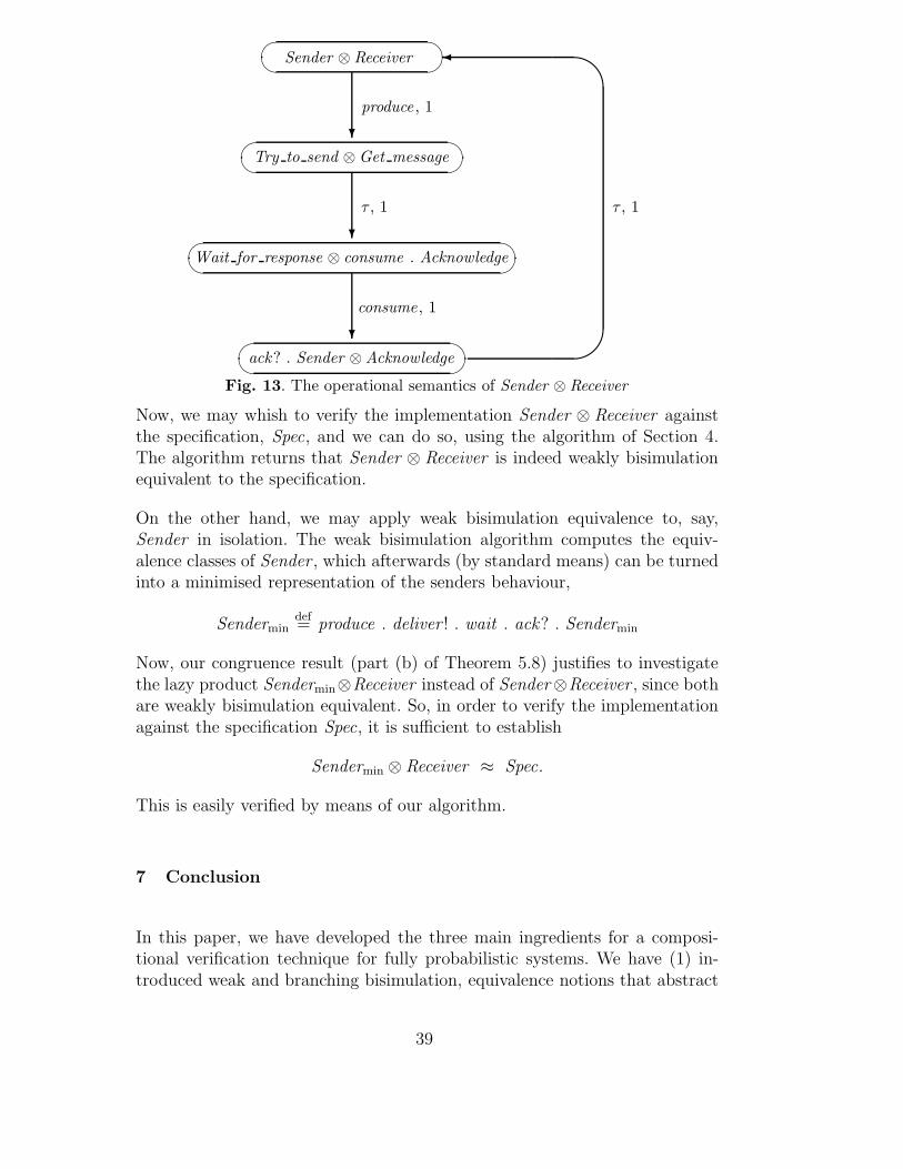
Sender ⊗ Receiver

Try to send ⊗Get message

Wait for response ⊗ consume . Acknowledge

ack? . Sender ⊗ Acknowledge

produce , 1

τ , 1 τ , 1

consume , 1

?

?

?

$

%

Fig. 13. The operational semantics of Sender ⊗ Receiver

Now, we may whish to verify the implementation Sender ⊗ Receiver againstthe specification, Spec, and we can do so, using the algorithm of Section 4.The algorithm returns that Sender ⊗ Receiver is indeed weakly bisimulationequivalent to the specification.

On the other hand, we may apply weak bisimulation equivalence to, say,Sender in isolation. The weak bisimulation algorithm computes the equiv-alence classes of Sender , which afterwards (by standard means) can be turnedinto a minimised representation of the senders behaviour,

Sendermindef= produce . deliver ! . wait . ack? . Sendermin

Now, our congruence result (part (b) of Theorem 5.8) justifies to investigatethe lazy product Sendermin⊗Receiver instead of Sender⊗Receiver , since bothare weakly bisimulation equivalent. So, in order to verify the implementationagainst the specification Spec, it is sufficient to establish

Sendermin ⊗ Receiver ≈ Spec.

This is easily verified by means of our algorithm.

7 Conclusion

In this paper, we have developed the three main ingredients for a composi-tional verification technique for fully probabilistic systems. We have (1) in-troduced weak and branching bisimulation, equivalence notions that abstract

39

QQQQ

QQQQ

≡ ≈

=ste

=wte

=tr

≡0

∼

≈br

Fig. 14. Position of weak bisimulation equivalence (≈) compared to other weakequivalences, cf. Section 3.3.

from internal computations. We have (2) introduced a calculus PLSCCS thatcan be used for specifying fully probabilistic systems, and that enjoys thecompositionality property with respect to weak (and branching) bisimulation.In addition, we have (3) illustrated that mechanised verification (and min-imisation) is feasible, by developing an algorithm to compute the weak (andbranching) bisimulation equivalence classes. The algorithm has a cubic timecomplexity, which meets the worst case complexity of branching bisimulationequivalence in the non-probabilistic setting.

These three ingredients form the basis to alleviate the state-space explosionproblem by generating the state space in a compositional fashion, where thealgorithm is applied to minimize the intermediate state spaces of components.Furthermore, the concept of lazy synchrony in isolation already helps to allevi-ate the state space explosion, since the effect of internal moves is by definitioncumulated with successing visible actions. We are intending to study in whatsense this beneficial side result can be transferred back to the non-probabilisticsetting.

Apart from its practical interest for compositional analysis of fully proba-bilistic systems, weak bisimulation equivalence enjoys a central position withrespect to other weak relations studied in the literature. Summarising theresults of Section 3.3 yields the lattice in Figure 14, where two relations areconnected by a line if the upper is contained in the lower. Weak and branchingbisimulation equivalence are connected by a horizontal line, since they agree.The crossed line between ≡ and ≈ indicates that both are incomparable.

The proofs of our main results rely on the regularity of certain matrices (withcolumns and rows for each state of the underlying system). Thus, the mainresults are only established for finite systems. It is an open question whetherour results carry over to arbitrary fully probabilistic systems (with possiblyinfinitely many states).

40

A Proofs of the main theorems

In this appendix we give the proofs of the main results of this paper. Inwhat follows, we fix a finite fully probabilistic system (S,Act ,P). We usethe following notations: If R is an equivalence relation on S and Ω a regularexpression such that Prob(s, Ω, C) = Prob(s′, Ω, C) for all (s, s′) ∈ R andC ∈ S/R then we define for all A ∈ S/R: Prob(A,Ω,C) = Prob(s, Ω, C)where s ∈ A. We simply write [s] to denote the weak bisimulation equivalenceclass of s (i.e. [s] = [s]≈).

A.1 Weak and branching bisimulation

In this section we give the proof of Theorem 3.9 stating that weak and branch-ing bisimulation equivalence coincide, and the proof of Theorem 3.5.

Definition A.1 Let R be a weak bisimulation. R is called complete iff

• Whenever s ∈ S, C ∈ S/R and Prob(s, τ ∗, C) = 1 then s ∈ C.• If Sdiv 6= ∅ then Sdiv ∈ S/R.

Note that, if R is a complete weak bisimulation and A ∈ S/R, A 6= Sdiv , thenA ∩ Sdiv = ∅ (in particular, A does not contain terminal states) and there isa state s ∈ A with P(s, τ, A) < 1. Thus, A ∩ SXns 6= ∅ where X = S/R is theinduced partition.(Recall that SXns is the set of non-silent states with respectto X .)

Lemma A.2 s ≈ s′ iff (s, s′) ∈ R for some complete weak bisimulation R.

Proof: It suffices to show that each weak bisimulation is contained in somecomplete weak bisimulation. For R to be a weak bisimulation, we define J (R)to be the smallest equivalence relation on S which contains R and such that:

• If Prob(s, τ ∗, [s′]R) = 1 then (s, s′) ∈ J (R)• If Sdiv 6= ∅ then (s, s′) ∈ J (R) for all s, s′ ∈ Sdiv .

Let R0 = R, Ri+1 = J (Ri) and R′ =⋃iRi. It is easy to see that R′ is a

complete weak bisimulation.

Definition A.3 For R to be a complete weak bisimulation, we define matricesAR and A0

R as follows: Let A1, . . . , Ak be an enumeration of those equivalenceclasses Ai ∈ S/R which contain some state si ∈ S \Sterm with P(si, τ, Ai) < 1.(Since R is complete, A1, . . . , Ak = S/R \ Sdiv.) Let AR be the following

41

matrix:AR = ( Prob(Ai, τ

∗, Aj) )1≤i,j≤k

We define A0 = Sdiv . In the case where A0 = ∅ we define Prob(A0, τ∗, A0) = 1

andProb(A0, τ

∗, Aj) = Prob(Aj , τ∗, A0) = 0

if j ≥ 1. Let A0R = ( Prob(Ai, τ

∗, Aj) )0≤i,j≤k.

Regardless of whether Sdiv is empty or not, the matrix A0R is of the form

A0R =

1 0 · · · 0

0... AR

0

.

Note that Sterm ⊆ Sdiv = A0. Hence, Ai ∩ Sterm = ∅, i = 1, . . . , k.

Lemma A.4 If R is a complete weak bisimulation then AR and A0R are reg-

ular. Moreover: For all l ∈ 1, . . . , k and all b0, . . . , bl−1, bl+1, . . . , bk ∈ [0, 1],the equation system

xl = 0,k∑i=0

xi · Prob(Ai, τ∗, Aj) = bj , j = 0, . . . , k, j 6= l

has at most one solution.

Proof: Let A0, . . . , Ak be as in Definition A.3. For each h ∈ 1, . . . , k wefix some state sh ∈ Ah with P(sh, τ, Ah) < 1. Let

C = ( P(sh, τ, Ai) )1≤h,i≤k and E =

1− e1 0 0 · · · 0

0 1− e2 0 · · · 0

0 0 1− e2 · · · 0

......

.... . .

...

0 0 0 · · · 1− ek

where

ej =k∑i=1

P(sj, τ, Ai) · Prob(Ai, τ∗, Aj).

42

We show that C ·AR + E = AR. Let dh,j be the element of C ·AR + Ein the h-th row and j-th column.

• For j = 1, . . . , k we have:

dj,j =k∑i=1

P(sj, τ, Ai) ·Prob(Ai, τ∗, Aj) + 1−ej = 1 = Prob(Aj , τ

∗, Aj).

• For h, j = 1, . . . , k and h 6= j:

Prob(Ah, τ∗, Aj) = Prob(sh, τ

∗, Aj) =k∑i=1

P(sh, τ, Ai)·Prob(Ai, τ∗, Aj) = dh,j.

Note that Prob(A0, τ∗, Aj) = 0 for all j ≥ 1.

This yields C ·AR + E = AR. Thus, E = (I−C) ·AR where I denotesthe k × k-identity matrix. Next we show that ej < 1, j = 1, . . . , k.

• If Prob(Ai0, τ∗, Aj) 6= 0 for some i0 ∈ 1, . . . , k \ j with P(sj, τ, Ai0) > 0

then

ej ≤k∑i=1

i6=i0

P(sj, τ, Ai) + P(sj, τ, Ai0) · Prob(Ai0 , τ∗, Aj) < P(sj, τ) ≤ 1

since Prob(Ai0, τ∗, Aj) < 1 because R is complete.

• If Prob(Ai, τ∗, Aj) = 0 for all i ∈ 1, . . . , k \ j with P(sj, τ, Ai) > 0 then

ej = P(sj, τ, Aj) · Prob(Aj, τ∗, Aj) = P(sj, τ, Aj) < 1.

Thus, in both cases, ej < 1. Hence, E is regular which yields the regularity ofAR. It is clear that the regularity of AR implies the regularity of the matrixA0R. Recall that A0

R (and thus the inverse matrix (AR0)−1 of A0

R) are of theform:

A0R =

1 0 . . . 0

0... AR

0

(AR

0)−1 =

1 0 . . . 0

0... A−1

R

0

Moreover, E ·A−1

R = I−C. Thus, (1− ej) · aj,j = 1−P(sj, τ, Aj) > 0 where(AR

0)−1 = (ai,j)0≤i,j≤1. Hence,

(*) aj,j > 0, j = 1, . . . , k.

Next we show that the equation system of above has at most one solution. Let

L = (b0, . . . , bl−1, t, bl+1, . . . , bk) : t ∈ IR

43

where IR denotes the set of real numbers. Let H = (x0, . . . , xk) ∈ IRk+1 :xl = 0 and L′ = y · (AR

0)−1 : y ∈ L. Then, H ∩ L′ is the set of solutionof the equation system under consideration. We show that either H ∩ L′ = ∅or H ∩ L′ consists of a single point. First we observe that H and L (and thusL′ and H ∩L′) are affine spaces with dim(H) = k and dim(L) = dim(L′) = 1where dim(X) denotes the dimension of X. Hence, if H ∩ L′ 6= ∅ then

• either dim(H ∩ L′) = 0 (iff H ∩ L′ consists of a single point)• or dim(H ∩ L′) = 1 (iff L′ ⊆ H).

Therefore, it suffices to show that L′ 6⊆ H . We suppose that L′ ⊆ H . Then,there are real vectors a, c such that L′ = a + t · c : t ∈ IR where a =(a0, . . . , ak) and c = (c0, . . . , ck) with al = cl = 0 and c 6= 0. By definition ofL′ we have L = x ·A0

R : x ∈ L′. Hence,

bj =k∑i=0

ai · Prob(Ai, τ∗, Aj) + t ·

k∑i=0

ci · Prob(Ai, τ∗, Aj)

for all j = 0, . . . , k, j 6= l and t ∈ IR. Thus,

k∑i=0

ci · Prob(Ai, τ∗, Aj) = 0 if j 6= l.

Hence,

cdef=

k∑i=0

ci · Prob(Ai, τ∗, Al) 6= 0

(since, otherwise the rows of A0R would be linear dependent in contradiction

to the regularity of A0R). W.l.o.g. c = 1. Then, c is the l-th row of (AR

0)−1.In particular, 0 = cl = al,l. But this contradicts the constraint al,l > 0 from(*).

We show that ≈ coincides with another kind of bisimulation equivalence thatwe call delay bisimulation, in analogy to [26].

Definition A.5 A delay bisimulation is an equivalence relation R on S suchthat Prob(s, τ ∗a, C) = Prob(s′, τ ∗a, C) for all (s, s′) ∈ R, a ∈ Act and allequivalence classes C ∈ S/R. s ≈dl s′ iff (s, s′) ∈ R for some delay bisimula-tion R.

Lemma A.6 s ≈dl s′ implies s ≈ s′. More precisely: Each delay bisimula-tion is a weak bisimulation.

Proof: Let R be a delay bisimulation. We show that R is a weak bisimu-lation. Let α ∈ Act \ τ, s ∈ S and C ∈ S/R. Then, for all B ∈ S/R ands ∈ B:

44

Prob(s, τ ∗ατ ∗, C) =∑t∈S

Prob(s, τ ∗α, t) · Prob(t, τ ∗, C)

=∑

A∈S/RProb(B, τ ∗α,A) · Prob(A, τ ∗, C).

Hence, if (s, s′) ∈ R then Prob(s, τ ∗ατ ∗, C) = Prob(s′, τ ∗ατ ∗, C) for allC ∈ S/R and α ∈ Act \ τ.

Lemma A.7 s ≈ s′ implies s ≈dl s′. More precisely: Each complete weakbisimulation is a delay bisimulation.

Proof: Let R be a complete weak bisimulation. We fix some α ∈ Act \ τand show that Prob(s, τ ∗α,A) = Prob(s′, τ ∗α,A) for all s ≈ s′ and allA ∈ S/R. (Ranging over all α, we obtain that R is a delay bisimulation. Thus,≈ ⊆ ≈dl.)

By the regularity of A0R (Lemma A.4): Whenever we fix a real vector a (of

length k+1) then the linear equation system x ·A0R = a has a unique solution.

For s ∈ S and j = 0, 1, . . . , k we have:

Prob(s, τ ∗ατ ∗, Aj) =∑t∈S

Prob(s, τ ∗α, t) · Prob(t, τ ∗, Aj)

=k∑i=0

Prob(s, τ ∗α,Ai) · Prob(Ai, τ∗, Aj).

Thus, for fixed l: For all states s ∈ Al, the vector (Prob(s, τ ∗α,Ai))0≤i≤k is asolution of the linear equation system x · A0

R = a where a = (aj)0≤j≤k andaj = Prob(Al, τ

∗ατ ∗, Aj). By the regularity of A0R: If (s, s′) ∈ R (i.e. s, s′ ∈ Al

for some l) then Prob(s, τ ∗α,Ai) = Prob(s′, τ ∗α,Ai), i = 0, . . . , k.

Proposition A.8 s ≈ s′ iff s ≈dl s′

Proof: follows by Lemma A.6 and Lemma A.7.

Lemma A.9 s ≈br s′ implies s ≈ s′. More precisely: Each branchingbisimulation is a weak bisimulation.

Proof: Let R be a branching bisimulation. It suffices to show that R is adelay bisimulation (Lemma A.6). For r ≥ 1 and A, C ∈ S/R, A 6= C, let Γrbe the set of tuples (C0, . . . , Cr) such that

• Ci ∈ S/R, i = 0, 1, . . . , r,• C0 = A, Cr = C,• Ci 6= Ci+1, i = 0, . . . , r − 1.

45

Then, for all s ∈ A:

Prob(s, τ ∗, C) =∞∑r=1

∑(C1,...,Cr)∈Γr

r−1∏i=0

ProbR(Ci, τ∗, Ci+1)

Hence, Prob(s, τ ∗, C) = Prob(s′, τ ∗, C) for all s, s′ ∈ A. Similarly,

Prob(s, τ ∗α,C) = Prob(s′, τ ∗α,C)

for all s, s′ ∈ A, α ∈ Act \ τ and C ∈ S/R.

Lemma A.10 Let R be an equivalence relation on S. Then, R is a branchingbisimulation if and only if for all C ∈ S/R, a ∈ Act and (s, s′) ∈ R:

(1) If P(s, τ, [s]R), P(s′, τ, [s′]R) < 1 and (a, C) 6= (τ, [s]R) then

P(s, a, C)

1−P(s, τ, [s]R)=

P(s′, a, C)

1−P(s′, τ, [s′]R).

(2) If P(s, τ, [s]R) = 1 then• either P(t, τ, [t]R) = 1 for all t ∈ [s]R• or there exists a finite path σ starting in s with σ(i) ∈ [s]R, i = 1, . . . , |σ|

and P(last(σ), τ, [s]R) < 1.

Proof: Let T = Sterm ∪ t ∈ S : P(t, τ, [t]R) = 1 (i.e. T is the set of silentstates T = S \ SXns with respect to X = S/R).

“if”: Let A ∈ S/R with A ⊆ T . Then, for all s ∈ A:

ProbR(s, τ ∗a, C) =

1 : if a = τ and C = A

0 : otherwise

Then, ProbR(t, τ ∗a, C) = ProbR(t′, τ ∗a, C) for all t, t′ ∈ A. Let A, C ∈ S/Rsuch that A 6⊆ T . Then, the matrix I−CA is regular where I is the |A| × |A|-identity matrix and CA = (P(s, τ, t))s,t∈A. This can be seen as follows: If(I − CA) · x = 0, x = (xs)s∈A, then xs =

∑t∈A P(s, τ, t) · xt for all s ∈ A.

If we suppose that x 6= 0 then we may assume w.l.o.g. that xs > 0 for somes ∈ A (otherwise we deal with −x rather than x). Let W be the set of statess ∈ A where xs is maximal. Then, for all s ∈W , P(s, τ, A) = 1 and xs = xt ifP(s, τ, t) > 0. Thus, W ⊆ T and, if s ∈ W then P(s, τ, t) > 0 implies t ∈ W .Hence, there is no finite path σ starting in s with σ(i) ∈ A, i = 0, 1, . . . , |σ|−1,and P(last(σ), τ, A) < 1. This contradicts (2).

Let a ∈ Act such that (a, C) 6= (τ, A). Then,

ProbR(s, τ ∗a, C) =∑t∈A

P(s, τ, t) · ProbR(t, τ ∗a, C) + P(s, a, C).

46

Hence, the vector (ProbR(s, τ ∗a, C))s∈A solves the equation system (I−CA) ·x = b where b = (bs)s∈A and bs = P(s, a, C). On the other hand, for all s ∈ A:

(*) P(s, a, C) = =∑t∈A

P(s, τ, t) ·P(s, a, C) + P(s, a, C)(1−P(s, τ, A)).

Let x = P(s, a, C)/(1−P(s, τ, A)) where s ∈ A \ T . (*) yields:

x =∑t∈A

P(s, τ, t) · x + P(s, a, C) for all s ∈ A.

(Note that P(s, a, C) = 0 and P(s, τ, A) = 1 for s ∈ A ∩ T .) Hence, thevector x = (xs)s∈A where xs = x for all s ∈ A solves the equation system(I − CA) · x = b. By the regularity of I − CA we get ProbR(s, τ ∗a, C) = xfor all s ∈ A. This yields that R is a branching bisimulation and

ProbR(s, τ ∗a, C) = x =P(s, a, C)

1−P(s, τ, A)

for all s ∈ A \ T .

“only if”: Let R be a branching bisimulation, A, C ∈ S/R and a ∈ Act suchthat (a, C) 6= (τ, A). Let

xa,C = ProbR(A, τ ∗a, C).

Then, xa,C = P(s, τ, A) · xa,C + P(s, a, C) for all s ∈ A. Hence, if s ∈ A∩Tthen

xa,C =P(s, a, C)

1−P(s, τ, A).

If s ∈ A ∩ T and A 6⊆ T then xa,C 6= 0 for some pair (a, C) as above. Thus,

ProbR(s, τ ∗a, C) = xa,C > 0.

Then, there exists a finite path σ′ starting in s of length r ≥ 1 with trace(σ′) ∈τ ∗a, σ′(i) ∈ A, i = 0, 1, . . . , r − 1 and last(σ′) ∈ C. Let σ be the (r − 1)-thprefix of σ′. Then, σ(i) ∈ A, i = 1, . . . , r − 1 and P(last(σ), τ, A) < 1 (sinceP(last(σ), a, C) > 0).

Lemma A.11 Let R be a branching bisimulation on S. If s ∈ S withP(s, τ, [s]R) < 1 then

ProbR(s, τ ∗a, C) =P(s, a, C)

1−P(s, τ, C)

for all a ∈ Act, C ∈ S/R with (a, C) 6= (τ, [s]R).

Definition A.12 Let R be an equivalence relation on S.

PR : S × Act × S −→ [0, 1]

47

is given by: PR(s, a, t) = 0 if P(s, τ, [s]R) = 1 or s ∈ Sterm . For s ∈ S \ Sterm

with P(s, τ, [s]R) < 1,

PR(s, a, t) =P(s, a, t)

1−P(s, τ, [s]R)if a 6= τ or t /∈ [s]R.

and PR(s, τ, t) = 0 if t ∈ [s]R. For C ⊆ S, a ∈ Act and s ∈ S, let

PR(s, a, C) =∑t∈C

PR(s, a, t).

Clearly, PR(·) = PX (·) (defined as in Definition 4.2 for the induced partitionX = S/R.

Lemma A.13 s ≈ s′ implies s ≈br s′. More precisely: Each complete weakbisimulation is a branching bisimulation.

Proof: Let R be a complete weak bisimulation. It suffices to show that Rfulfills the conditions (1), (2) of Lemma A.10. As in the proof of that lemma,let T = Sterm ∪ t ∈ S : P(t, τ, [t]R) = 1.

Condition (2): Let A ∈ S/R, A 6= Sdiv . There exists a ∈ Act and C ∈ S/Rwith (τ, A) 6= (a, C) such that Prob(A, τ ∗a, C) 6= 0. Hence, for each s ∈ Tthere is a finite path σ with trace(σ) ∈ τ ∗a and last(σ) ∈ C. Let i be thesmallest index such that σ(i) /∈ T . (Such an index i exists by definition of T .)Then, i ≥ 1 and σ(i) ∈ A \ T . (Note that σ(i− 1) ∈ T implies σ(i) ∈ A.)

Condition (1): Let A0, . . . , Ak be as in Definition A.3. Let C ∈ S/R, Aj 6= C,s ∈ Aj. Then,

Prob(s, τ ∗, C) =k∑i=0

P(s, τ, Ai) · Prob(Ai, τ∗, C).

Note that Prob(C, τ ∗, C) = 1. Now we suppose that s ∈ Aj \ T . Then,

Prob(s, τ ∗, C)

1−P(s, τ, Aj)=

k∑i=0

P(s, τ, Ai)

1−P(s, τ, Aj)· Prob(Ai, τ

∗, C)

=k∑i=0

i6=j

P(s, τ, Ai)

1−P(s, τ, Aj)· Prob(Ai, τ

∗, C) +P(s, τ, Aj)

1−P(s, τ, Aj)· Prob(Aj , τ

∗, C)

=k∑i=0

i6=j

PR(s, τ, Ai) · Prob(Ai, τ∗, C) +

P(s, τ, Aj)

1−P(s, τ, Aj)· Prob(s, τ ∗, C)

Here, we use the fact that Prob(s, τ ∗, C) = Prob(Aj, τ∗, C). We obtain:

48

Prob(s, τ ∗, C) = Prob(s, τ ∗, C) ·(

1

1−P(s, τ, Aj)− P(s, τ, Aj)

1−P(s, τ, Aj)

)

=k∑i=0

i6=j

PR(s, τ, Ai) · Prob(Ai, τ∗, C)

Thus, for each s ∈ Aj \ T , the vector (PR(s, τ, Ai))0≤i≤k solves the equationsystem

xj = 0,k∑i=0

xi · Prob(Ai, τ∗, C) = Prob(Aj , τ

∗, C).

Lemma A.4 yields PR(s, τ, C) = PR(s′, τ, C) for all s, s′ ∈ Aj and C ∈ S/R,C 6= Aj . Let

PR(Aj, τ, C) = PR(s, τ, C) where s ∈ Aj ∩ T .

For all α ∈ Act \ τ and s ∈ Aj :

Prob(s, τ ∗α,C) =k∑i=0

P(s, τ, Ai) · Prob(Ai, τ∗α,C) + P(s, α, C)

As before, we obtain for s ∈ Aj \ T :

Prob(s, τ ∗α,C) =k∑i=0i6=j

PR(s, τ, Ai) · Prob(Ai, τ∗α,C) + PR(s, α, C).

Then, for all s ∈ Aj \ T , α ∈ Act and C ∈ S/R:

Prob(Aj, τ∗α,C) =

k∑i=0i6=j

PR(Aj, τ, Ai) · Prob(Ai, τ∗α,C) + PR(s, α, C)

We obtain PR(s, α, C) = PR(s′, α, C) for all s, s′ ∈ Aj \ T .

Corollary A.14 s ≈ s′ iff s ≈br s′.

Lemma A.15 Let R1, R2 be branching bisimulations. Then, R = (R1 ∪R2)∗

is a branching bisimulation.

Proof: We show that R fulfills the conditions (1) and (2) of Lemma A.10.First we observe that for j ∈ 1, 2, each equivalence class C ′ ∈ S/R can bewritten as C ′ = C0 ∪ . . . ∪ Cr where Ci ∈ S/Rj .

Condition (1): Let B, C0, . . . , Cr ∈ S/Rj such that Ci ∩ Ch = ∅ if i 6= h. Lets, s′ ∈ C0 with P(s, τ, C0), P(s′, τ, C0) < 1 and a ∈ Act with a 6= τ if C0 = Band C ′ = C0 ∪ . . . ∪ Cr. Then:

49

P(s, a, B) · (1−P(s′, τ, C ′)) = P(s, a, B) ·(

1−r∑i=0

P(s′, τ, Ci)

)

= P(s, a, B) ·(

1−P(s′, τ, C0)−r∑i=1

P(s, τ, Ci)

1−P(s, τ, C0)· (1−P(s′, τ, C0))

)

= (1−P(s′, τ, C0)) ·P(s, a, B) ·(

1−r∑i=1

P(s, τ, Ci)

1−P(s, τ, C0)

)

= P(s′, a, B) · (1−P(s, τ, C0)) ·(

1−r∑i=1

P(s, τ, Ci)

1−P(s, τ, C0)

)

= P(s′, a, B) ·(

1−r∑i=0

P(s, τ, Ci)

)= P(s′, a, B) · (1−P(s, τ, C ′))

Now we assume that C ′ ∈ S/R. Hence, for all B′ ∈ S/R, a ∈ Act such thata 6= τ if C0 ⊆ B′: If P(s, τ, C ′), P(s′, τ, C ′) < 1. then:

P(s, a, B′)

1−P(s, τ, C ′)=

r∑i=0

P(s, a, Bi)

1−P(s, τ, C ′)=

r∑i=0

P(s′, a, Bi)

1−P(s′, τ, C ′)=

P(s′, a, B′)

1−P(s′, τ, C ′)

if B′ = B0 ∪ . . . ∪ Bm where Bi ∈ S/Rj and Bi ∩ Bh = ∅ if i 6= h.

Condition (2): Let P(s, τ, [s]R) = 1. We may assume that P(s, τ, [s]Rj) < 1,j = 1, 2, and that P(t, τ, C ′) < 1 for some t ∈ C ′ where C ′ = [s]R. (In the casewhere P(s, τ, [s]Rj) = 1 for some j we apply Lemma A.10 to Rj and obtainthe claim.) There is some a ∈ Act , B′ ∈ S/R with B′ 6= C ′ if a = τ andP(t, a, B′) > 0. By definition of R there is a sequence s = s0, s1, . . . , sl = twith (si, si+1) ∈ R1 ∪ R2, i = 1, . . . , l. It can easily shown by induction on ithat Prob(si, τ

∗a, B′) > 0, i = 0, . . . , l, Hence, there is a finite path σ withfirst(σ) = s, σ(i) ∈ C ′, i = 0, 1, . . . , |σ| and P(last(σ), τ, C ′) < 1.

Lemma A.16 ≈br is a branching bisimulation.

Proof: Let R1, . . . , Rr be an enumeration of all branching bisimulations(on the fixed fully probabilistic system (S,Act ,P)). Let R = (

⋃iRi)

∗. Byinduction on r and using Lemma A.15, it can be shown that R is a branchingbisimulation. Thus, R ⊆ ≈br. On the other hand, ≈br =

⋃iRi (by definition

of ≈br). Hence, ≈br ⊆ R. Thus, ≈br = R is a branching bisimulation.

Lemma A.17 ≈ is a weak bisimulation.

Proof: Lemma A.9, Lemma A.16 and Corollary A.14 yield that ≈ = ≈bris a weak bisimulation.

Theorem A.18 If s ≈ s′. then, for all C ∈ S/ ≈, k ≥ 1 and α1, . . . , αk ∈Act \ τ:

50

(a) Prob(s, τ ∗α1τ∗α2τ

∗ . . . τ ∗αk, C) = Prob(s′, τ ∗α1τ∗α2τ

∗ . . . τ ∗αk, C),(b) Prob(s, τ ∗α1τ

∗α2τ∗ . . . τ ∗αkτ

∗, C) = Prob(s′, τ ∗α1τ∗α2τ

∗ . . . τ ∗αkτ∗, C).

Proof: We prove part (a) by induction on k. In the basis of induction(k = 1) we have to show that Prob(s, τ ∗α,C) = Prob(s′, τ ∗α,C) for all visibleactions α and all weak bisimulation equivalence classes C. This follows imme-diately by Proposition A.8 and Lemma A.17. In the induction step k−1 =⇒ kwe assume that k ≥ 2, α1, . . . , αk ∈ Act \ τ and Ω = τ ∗α2τ

∗ . . . τ ∗αk. Then,

• Prob(t, Ω, C) = Prob(t′, Ω, C) for all t ≈ t′ and C ∈ S/ ≈• Prob(s, τ ∗α1, A) = Prob(s′, τ ∗α1, A) for all A ∈ S/ ≈

(induction hypothesis). Thus:

Prob(s, τ ∗α1Ω,C) =∑

A∈S/≈Prob(s, τ ∗α1, A) · Prob(A,Ω,C)

=∑

A∈S/≈Prob(s′, τ ∗α1, A) · Prob(A,Ω,C) = Prob(s′, τ ∗α1Ω,C).

Here, we use the fact that Path ful(u, τ∗α1Ω,C) can be written as disjoint union

of the sets ΠA(u), A ∈ S/ ≈, where ΠA is the set of fulpaths π such that

• trace(π(k)) ∈ τ ∗α1,• π(k) ∈ A,• π = π(k) γ where γ ∈ Path ful (π(k), Ω, C)

for some k ≥ 0. Part (b) can be derived from (a):

Prob(s, Ω, C) =∑

A∈S/≈Prob(s, τ ∗α1τ

∗ . . . τ ∗αk, A) · Prob(A, τ ∗, C)

=∑

A∈S/≈Prob(s′, τ ∗α1τ

∗ . . . τ ∗αk, A) · Prob(A, τ ∗, C) = Prob(s′, Ω, C).

where Ω = τ ∗α1τ∗ . . . τ ∗αkτ

∗.

A.2 Weak bisimulation and the testing equivalences =ste and ≡0

We complete the proofs of Theorem 3.12 and Theorem 3.13 by showing that≈ is finer than the testing equivalences =ste and ≡0.

Lemma A.19 If A, C ∈ S/ ≈, s, s′ ∈ A, L ⊆ Act \ τ and α ∈ L then

Q(s, L, α, C) = Q(s′, L, α, C).

51

Proof: First we observe that, for all A, B ∈ S/ ≈ = S/ ≈br, s, s′ ∈ Awith P(s, τ, A), P(s′, τ, A) < 1 and α ∈ Act \ τ:

• P(s, τ, S \ A) + P(s, L)

1−P(s, τ, A)=

P(s′, τ, S \ A) + P(s′, L)

1−P(s′, τ, A)

• P(s, α, B)

1−P(s, τ, A)=

P(s′, α, B)

1−P(s′, τ, A)

In particular, P(s, τ, S \A) + P(s, L) = 0 iff P(s′, τ, S \A) + P(s′, L) = 0.If A = Sdiv then we put P′(A, α,B) = 0 and rA = 1. For A ∈ S/ ≈, A 6= Sdiv ,we define

P′(A, α,B) =P(s, α, B)

1−P(s, τ, A), rA =

P(s, τ, S \ A) + P(s, L)

1−P(s, τ, A)

where s ∈ A such that P(s, τ, A) < 1. Let (qA)A∈S/≈ be the unique solution ofthe following equation system.

1. qA = 0 if rA = 0 or Prob(A, τ ∗α,C) = 0.2. If rA > 0 and Prob(A, τ ∗α,C) > 0 then

qA =1

rA·

P′(A, α, C) +∑

B∈S/≈B 6=A

P′(A, τ, B) · qB

.

The uniqueness of the equation system above is an easy verification. For allA ∈ S/ ≈ such that rA > 0 and Prob(A, τ ∗α,C) > 0 and s ∈ A withP(s, τ, A) > 0 we have:

P(s, τ, S \ A) + P(s, L) > 0

and

(1− P(s, τ, A)

P(s, τ) + P(s, L)

)· qA =

P(s, τ, S \ A) + P(s, L)

P(s, τ) + P(s, L)· qA

=P(s, τ, S \ A) + P(s, L)

P(s, τ) + P(s, L)· 1

rA·

P′(A, α, C) +∑

B∈S/≈B 6=A

P′(A, τ, B) · qB

=1−P(s, τ, A)

P(s, τ) + P(s, L)·

P′(A, α, C) +∑

B∈S/≈B 6=A

P′(A, τ, B) · qB

52

=1

P(s, τ) + P(s, L)·

P(s, α, C) +∑

B∈S/≈B 6=A

P(A, τ, B) · qB

=

P(s, α, C)

P(s, τ) + P(s, L)+

∑B∈S/≈B 6=A

P(s, τ, B)

P(s, τ) + P(s, L)· qB.

Thus,

qA =P(s, α, C)

P(s, τ) + P(s, L)+

∑B∈S/≈

P(s, τ, B)

P(s, τ) + P(s, L)· qB.

For A ∈ S/ ≈ and s ∈ A, let qs = qA and rs = rA. Then, the vector (qs)s∈Ssolves the following regular linear equation system. If Prob(s, τ ∗α,C) = 0 orrs = 0 then qs = 0. Otherwise,

qs =P(s, α, C)

P(s, τ) + P(s, L)+

∑u∈S

P(s, τ, u)

P(s, τ) + P(s, L)· qu.

It is easy to see that, if rs = 0 then Q(s, L, α, C) = 0. Thus, the vector(Q(s, L, α, C))s∈S is also a solution of the equation system above. Hence,

qs = Q(s, L, α, C) for all s ∈ S.

We conclude: Q(s, L, α, C) = qA = Q(s′, L, α, C) for all s, s′ ∈ A, A ∈ S/ ≈.

Theorem A.20 ≈ is finer than =ste.

Proof: As observed in [15], s =ste s′ iff

Q(s, L1 . . . Lk, α1 . . . αk) = Q(s′, L1 . . . Lk, α1 . . . αk)

for all L1, . . . , Lk ∈ Offr and α1, . . . , αk ∈ Act \ τ. By induction on k andusing Lemma A.19 we obtain that, if s ≈ s′ then

Q(s, L1 . . . Lk, α1 . . . αk, C) = Q(s′, L1 . . . Lk, α1 . . . αk, C)

for all C ∈ S/ ≈. Summing up over all C ∈ S/ ≈ we obtain

Q(s, L1 . . . Lk, α1 . . . αk) = Q(s′, L1 . . . Lk, α1 . . . αk).

Hence, s =ste s′.

Definition A.21 For X to be a set, let Distr0(X) be the set consisting of alldistributions on X and the function ρ : X −→ [0, 1] with ρ(x) = 0 for allx ∈ X.

53

Definition A.22 A probabilistic trace is a finite sequence

θ = 〈ρ1, α1〉〈ρ2, α2〉 . . . 〈ρk, αk〉

over Distr 0(Act \ τ) × (Act \ τ). εPrTr denotes the empty probabilistictrace, ProbTraces the collection of all probabilistic traces.

Definition A.23 For ρ ∈ Distr 0(Act \ τ) and s ∈ S, the normalizator ofs and ρ is defined by

norm(s, ρ) =∑

α∈Act\τP(s, α) · ρ(α) + P(s, τ).

[19,73] define the probabilities N(s, α, ρ, C) that from state s the state t isreached via a finite path labelled by τ ∗α given that the environment is enablingactions accordance with ρ. Here, we use a slightly different way to define N(·)(which yields the same values).

Definition A.24 Let

N : S × (Act \ τ)×Distr 0(Act \ τ)× 2S −→ [0, 1]

be defined as follows. The vector (N(s, α, ρ, C))s∈S is the unique solution ofthe following linear equation system:

1. If Prob(s, τ ∗α,C) = 0 or norm(s, ρ) = 0 then N(s, α, ρ, C) = 0.2. If Prob(s, τ ∗α,C) > 0 and norm(s, ρ) > 0 then

N(s, α, ρ, C) =ρ(α)

norm(s, ρ)·P(s, α, C) +

∑t∈S

P(s, τ, t)

norm(s, ρ)·N(t, α, ρ, C).

Clearly, if ρ(α) = 0 for all α then N(s, α, ρ, C) = 0 for all states s and C ⊆ S.

Definition A.25 Let M : S × ProbTraces −→ [0, 1] be given by:M(s, εPrTr) = 1 and

M(s, 〈ρ, α〉θ) =∑t∈S

N(s, α, ρ, t) ·M(t, θ)

We define s ≡0 s′ iff M(s, θ) = M(s′, θ) for all θ ∈ ProbTraces.

Lemma A.26 If s ≈ s′ then N(s, α, ρ, C) = N(s′, α, ρ, C) for all α ∈Act \ τ, ρ ∈ Distr 0(Act \ τ and C ∈ S/ ≈.

Proof: If ρ(α) = 0 for all α then N(s, α, ρ, C) = N(s′, α, ρ, C) = 0. Nowwe assume that ρ ∈ Distr(Act \ τ). For A ∈ S/ ≈, A 6= Sdiv , we choosesome s ∈ A with P(s, τ, A) < 1 and define

54

P′(A, a, C) =P(s, α, C)

1−P(s, τ, A)for (a, C) 6= (τ, A),

P′(A, τ) =∑

C∈S/≈C 6=A

P′(A, τ, C), P′(A, α) =∑

C∈S/≈P′(A, α, C).

We define P′(Sdiv , τ) = 0 and P′(Sdiv , a, C) = 0 if (a, C) 6= (τ, Sdiv). For allA ∈ S/ ≈ we define:

norm(A, ρ) =∑

α∈Act\τP′(A, α) · ρ(α) + P′(A, τ).

First we show that

(1) norm(A, ρ) = 0 implies Prob(s, τ ∗α) = 0 for all s ∈ A and α ∈ Act \ τwith ρ(α) > 0.

Let norm(A, ρ) = 0 and α ∈ Act \ τ with ρ(α) > 0. Then:

• P′(A, α, C) = 0 for all C ∈ S/ ≈,• P′(A, τ, C) = 0 for all C ∈ S/ ≈, C 6= A.

Hence, P(s, α) = 0 and P(s, τ, S \ A) = 0 for all s ∈ A. In particular,Prob(s, τ ∗, S \ A) = 0 for all s ∈ A. This yields Prob(s, τ ∗α) = 0.

For A, C ∈ S/ ≈, α ∈ Act \ τ and ρ ∈ Distr0(Act \ τ), we defineN(A, α, ρ, C) as follows. The vector (N(A, α, ρ, C))A∈S/≈ is the unique solutionof the linear equation system:

1. If norm(A, ρ) = 0 then N(A, α, ρ, C) = 0.2. If norm(A, ρ) > 0 then

N(A, α, ρ, C) =ρ(α)

norm(A, ρ)·P′(A, α, C) +

∑B∈S/≈B 6=A

P′(A, τ, t)

norm(A, ρ)·N(B, α, ρ, C).

In what follows, we suppose α, ρ and C to be fixed. It suffices to show that

(*) N(s, α, ρ, C) = N(A, α, ρ, C) for all s ∈ A and A ∈ S/ ≈.

For all s ∈ S we define xs = N([s], α, ρ, C). (Recall that [s] denotes the weakbisimulation equivalence class of s.) Clearly, (*) holds if norm(A, ρ) = 0. Nowwe assume A ∈ S/ ≈ and norm(A, ρ) > 0. (In particular, A 6= Sdiv .) Then:

(2) If s ∈ A with P(s, τ, A) < 1 then

norm(s, ρ)−P(s, τ, A) = norm(A, ρ) · (1−P(s, τ, A)) .

55

(3) If s ∈ A with P(s, τ, A) < 1 then norm(s, ρ) = P(s, τ, A) iff norm(A, ρ) =0.

First we assume that norm(A, ρ) = 0. By (1), Prob(s, τ ∗α) = 0 for all s ∈ A.Thus, by the definition of N(·), N(s, α, ρ, C) = 0 = N(A, α, ρ, C) = xs.

Next we assume that norm(A, ρ) > 0. It is easy to see that, ifProb(A, τ ∗α,C) = 0 then xs = 0 = N(A, α, ρ, C) for all s ∈ A. In whatfollows, we suppose Prob(A, τ ∗α,C) > 0. By (2) and (3),

• norm(s, ρ) > 0 for all s ∈ A,• norm(s, ρ) > P(s, τ, A) for all s ∈ A with P(s, τ, A) < 1.

Let s ∈ A with P(s, τ, A) < 1. Then:

xs =N(A, α, ρ, C)

=ρ(α)

norm(A, ρ)·∑t∈C

P(s, α, t)

1−P(s, τ, A)+

1

norm(A, ρ)·∑t∈S\A

P(s, τ, t)

1−P(s, τ, A)· xt

= ρ(α) · 1−P(s, τ, A)

norm(s, ρ)−P(s, τ, A)·∑t∈C

P(s, α, C)

1−P(s, τ, A)

+1−P(s, τ, A)

norm(s, ρ)−P(s, τ, A)·∑t∈S\A

P(s, τ, t)

1−P(s, τ, A)· xt

=ρ(α)

norm(s, ρ)−P(s, τ, A)·P(s, α, C)

+1

norm(s, ρ)−P(s, τ, A)·∑t∈S

P(s, τ, t) · xt −P(s, τ, A)

norm(s, ρ)−P(s, τ, A)· xs

Thus,

xs ·norm(s, ρ)

norm(s, ρ)−P(s, τ, A)= xs ·

(1 +

P(s, τ, A)

norm(s, ρ)−P(s, τ, A)

)

=1

norm(s, ρ)−P(s, τ, A)·(ρ(α) ·P(s, α, C) +

∑t∈S

P(s, τ, t) · xt).

Hence,

xs =ρ(α)

norm(s, ρ)·P(s, α, C) +

1

norm(s, ρ)·∑t∈S

P(s, τ, t) · xt.

This yields xs = N(s, α, ρ, C) for all s ∈ A.

56

Theorem A.27 ≈ is finer than ≡0.

Proof: follows by Lemma A.26 and induction on the length of the proba-bilistic traces.

References

[1] S. Abramsky, A. Jung: Domain Theory, In S. Abramsky, D.M. Gabbayand T.S.E. Maibaum (ed.), Handbook of Logic in Computer Science, Vol. 3,Clarendon Press, pp 1-168, 1994.

[2] A. Aho, J. Hopcroft, J. Ullman: The Design and Analysis of of ComputerAlgorithms, Addison-Wesley Publishing Company, 1974.

[3] S. Andova. Process algebra with probabilistic choice. In J.-P. Katoen, editor,Formal Methods for Real-Time and Probabilistic Systems, LNCS 1601, pages111–129, 1999.

[4] A. Aziz, V. Singhal, F. Balarin, R. Brayton, A. Sangiovanni-Vincentelli: Itusually works: The Temporal Logic of Stochastic Systems, Proc. CAV’95, LNCS939, pp 155-165, 1995.

[5] J. Baeten, J. Bergstra, S. Smolka: Axiomatizing Probabilistic Processes: ACPwith Generative Probabilities, Information and Computation, Vol. 122, pp 234-255, 1995.

[6] C. Baier: Polynomial Time Algorithms for Testing Probabilistic Bisimulationand Simulation, Proc. CAV’96, LNCS 1102, pp 38-49, 1996.

[7] C. Baier, H. Hermanns: Weak Bisimulation for Fully Probabilistic Processes,Proc. CAV’97, LNCS 1254, pp. 119-130, 1997.

[8] C. Baier: On algorithmic verification methods for probabilistic systems.Habilitation thesis, Univ. Mannheim, 1998.

[9] C. Baier, M. Stoelinga: Probabilistic Bisimulation and Simulation: Decidability,Complexity and Compositionality, in preparation.

[10] J. Bergstra, J. Klop: Process Algebra for Synchronous Communication,Information and Computation, Vol. 60, pp 109-137, 1984.

[11] G. Berry, G. Gonthier: The ESTEREL Synchronous Programming Language:Design, Semantics, Implementation, Science of Computer Programming,Vol. 19, 1992.

[12] A. Bianco, L. de Alfaro: Model Checking of Probabilistic and NondeterministicSystems, Proc. FST&TCS, LNCS 1026, pp 499-513, 1995.

[13] S. Campos: A Quantitative Approach to the Formal Verification of Real-TimeSystems, Ph.D.Thesis, Carnegie Mellon University, 1996.

57

[14] G. Chehaivbar, H. Garavel, N. Tawbi, F. Zulian: Specification and Verificationof the Powerscale Bus Arbitration Protocol: An Industrial Experiment withLOTOS, Formal Description Techniques IX, pp 435-450, Chapmann&Hall,1996.

[15] I. Christoff: Testing Equivalences and Fully Abstract Models for ProbabilisticProcesses: Proc. CONCUR’90, LNCS 458, pp 126-140, 1990.

[16] I. Christoff: Testing Equivalences for Probabilistic Processes, Ph. D. Thesis,Department of Computer Science, Uppsala University, 1990.

[17] L. Christoff, I. Christoff: Efficient Algorithms for Verification of Equivalencesfor Probabilistic Processes, Proc. CAV’91, LNCS 575, pp 310-321, 1991.

[18] E. Clarke, O. Grumberg, and D. Long: Model Checking and Abstraction, ACMTransactions on Programming Languages and Systems, Vol. 16, pp 1512-1542,1994.

[19] R. Cleaveland, S. Smolka, and A. Zwarico: Testing Preorders for ProbabilisticProcesses, Proc. ICALP 1992, LNCS 623, pp 708-719, 1992.

[20] D. Coppersmith, S. Winograd: Matrix Multiplication via ArithmeticProgressions, Proc. 19th ACM Symposium on Theory of Computing, pp 1-6,1987.

[21] C. Courcoubetis, M. Yannakakis: Verifying Temporal Properties of Finite-StateProbabilistic Programs, Proc. FOCS’88, pp 338-345, 1988.

[22] C. Courcoubetis, M. Yannakakis: The Complexity of Probabilistic Verification,Journal of the ACM, Vol. 42, No. 4, pp 857-907, 1995.

[23] P.R. D’Argenio, H. Hermanns, and J.-P. Katoen. On asynchronous generativeparallel composition. Proc. PROBMIV 98, Electronic Notes in TheoreticalComputer Science, Vol. 21, 1999.

[24] M. Fang, C. Ho-Stuart, H. Zedan: Specification of Real-Time ProbabilisticBehaviour, Proc. Protocol, Specification, Testing and Verification, IFIP,Elsevier Science Publishers, pp 143-157, 1993.

[25] A. Giacalone, C. Jou, S. Smolka: Algebraic Reasoning for ProbabilisticConcurrent Systems, Proc. IFIP TC2 Working Conference on ProgrammingConcepts and Methods, 1990.

[26] R.J. van Glabbeek: The Linear Time – Branching Time Spectrum II: Thesemantics of sequential systems with silent moves (Extended Abstract). Proc.CONCUR ’93, LNCS 715, pp 66–81. Springer, 1993.

[27] R.J. van Glabbeek, S. Smolka, B. Steffen: Reactive, Generative, and StratifiedModels for Probabilistic processes, Information and Computation, Vol. 121, pp59-80, 1995.

[28] R.J. van Glabbeek, W. Weijland: Branching Time and Abstraction inBisimulation Semantics, Journal of the ACM 43(3), pp 555-600,1996.

58

[29] C. Gregorio-Rodriguez, L. Llana-Diaz, M. Nunez, and P. Paloa-Gostanza.In M. Bertran and T. Rus, editors, Transformation-Based Reactive SystemsDevelopment, LNCS 1231, pages 353–367. Springer-Verlag, 1997.

[30] J.F. Groote, F. Vaandrager: An Efficient Algorithm for Branching Bisimulationand Stuttering Equivalence, Proc. ICALP’90, LNCS 443, pp 626-638, 1990.

[31] N. Halbwachs, F. Lagnier and C. Ratel. Programming and verifying criticalsystems by means of the synchronous data-flow programming language Lustre,IEEE Transactions on Software Engineering, 1992.

[32] H. Hansson: Time and Probability in Formal Design of Distributed Systems,Ph.D.Thesis, Uppsala University, 1991.

[33] H. Hansson, B. Jonsson: A Logic for Reasoning about Time and Probability,Formal Aspects of Computing, Vol. 6, pp 512-535, 1994.

[34] S. Hart, M. Sharir: Probabilistic Temporal Logic for Finite and BoundedModels, Proc. 16th ACM Symposium on Theory of Computing, pp 1-13, 1984.

[35] J. Hartog, E. de Vink: Mixing up Nondeterminism and Probability: aPreliminary Report, Proc. PROBMIV’98, Electronic Notes in TheoreticalComputer Science, Vol. 21, 1999.

[36] V. Hartonas-Garmhausen: Probabilistic Symbolic Model Checking withEngineering Models and Applications, Ph.D.Thesis, Carnegie Mellon University,1998.

[37] J. He, A. McIver, K. Seidel: Probabilistic Models for the Guarded CommandLanguage, Science of Computer Programming, Vol. 28, No. 2/3, pp 171-192,1997.

[38] M. Hennessy: Algebraic Theory of Processes, MIT Press, Boston, Mass., 1988.

[39] C.A.R. Hoare: Communicating Sequential Processes, Prentice Hall, 1985.

[40] ISO. LOTOS : A Formal Description Technique Based on the TemporalOrdering of Observational Behaviour, Standard IS 8807, TC97/SC21, 1989.

[41] B. Jonsson, K.G. Larsen: Specification and Refinement of ProbabilisticProcesses, Proc. LICS’91, pp 266-277, 1991.

[42] B. Jonsson, W. Yi: Compositional Testing Preorders for Probabilistic Processes,Proc. LICS’95, pp 431-443, 1995.

[43] C.C. Jou, S. Smolka, Equivalences, Congruences and Complete Axiomatizationsfor Probabilistic Processes, Proc. CONCUR’90, LNCS 458, pp 367-383, 1990.

[44] B. Jonsson, W. Yi: Compositional Testing Preorders for Probabilistic Processes,Proc. LICS’95, pp 431-443, 1995.

[45] P. Kanellakis, S. Smolka: CCS Expressions, Finite State Processes, and ThreeProblems of Equivalence, Information and Computation, Vol. 86, pp 43-68,1990.

59

[46] J.G. Kemeny and J.L. Snell. Finite Markov Chains. Springer, 1976.

[47] M. Kwiatkowska, G. Norman: A Fully Abstract Metric-Space DenotationalSemantics for Reactive Probabilistic Processes, Proc. COMPROX’98,Electronic Notes in Theoretical Computer Science, Vol. 13, 1998.

[48] K.G. Larsen, A. Skou: Bisimulation through Probabilistic Testing, Informationand Computation, Vol. 94, pp 1-28, 1991.

[49] K.G. Larsen, A. Skou: Compositional Verification of Probabilistic Processes,Proc. CONCUR’92, LNCS 630, pp 456-471, 1992.

[50] G. Lowe: Probabilities and Priorities in Timed CSP, Ph.D.Thesis, OxfordUniversity, 1993.

[51] R. Milner: A Calculus of Communicating Systems, LNCS 92, 1980.

[52] R. Milner: Calculi for Synchrony and Asynchrony, Theoretical ComputerScience, Vol. 25, pp 269-310, 1983.

[53] R. Milner: Communication and Concurrency, Prentice Hall, 1989.

[54] C. Morgan, A. McIver, K. Seidel, J. Sanders: Refinement-Oriented Probabilityfor CSP, Techn. Report TR-12-94, Oxford University, to appear in FormalAspects of Computing.

[55] R. de Nicola, M. Hennessy: Testing Equivalences for Processes, TheoreticalComputer Science, Vol. 34, pp 83-133, 1983.

[56] M. Nunez, D. de Frutos: Testing Semantics for Probabilistic LOTOS,Proc. Formal Description Techniques VIII, pp 365-380, Chapman&Hall, 1995.

[57] R. Paige, R. Tarjan: Three Partition Refinement Algorithms, SIAM Journal ofComputing, Vol. 16, No. 6, pp 973-989, 1987.

[58] D. Park: Concurrency and Automata on Infinite Sequences, Proc. 5th GIConference, LNCS 104, pp 167-183, 1981.

[59] A. Philippou, O. Sokolsky: Weak Bisimulation for Probabilistic Processes, 1998.

[60] A. Pnueli, L. Zuck: Verification of Multiprocess Probabilistic Protocols,Distributed Computing, Vol. 1, No. 1, pp 53-72, 1986.

[61] A. Pnueli, L. Zuck: Probabilistic Verification, Information and Computation,Vol. 103, pp 1-29, 1993.

[62] G.D. Plotkin. A Structured Approach to Operational Semantics. TechnicalReport DAIMI FM-19, Computer Science Department, Aarhus University, 1981.

[63] R. Segala: Modeling and Verification of Randomized Distributed Real-TimeSystems, Ph.D.Thesis, Massachusetts Institute of Technology, 1995.

[64] R. Segala, N. Lynch: Probabilistic Simulations for Probabilistic Processes,Proc. CONCUR’94, LNCS 836, pp 481-496, 1994.

60

[65] R. Segala, N. Lynch: Probabilistic Simulations for Probabilistic Processes,Nordic Journal of Computing, Vol. 2 (2), pp 250-273, 1995.

[66] K. Seidel: Probabilistic Communicating Processes, Theoretical ComputerScience, Vol. 152, pp 219-249, 1995.

[67] R. Sisto, L. Ciminiera, A. Valenzo: Probabilistic Characterization of AlgebraicProtocol Specifications, Proc. 12th International Conference on DistributedComputing Systems, pp 260-268, IEEE Comp. Soc. Press, 1992.

[68] S. Smolka, B. Steffen: Priority as Extremal Probability, Proc. CONCUR’90,LNCS 458, pp 456-466, 1990.

[69] S. Smolka, B. Steffen: Priority as Extremal Probability, Formal Aspects ofComputing, Vol. 8, pp 585-606, 1996.

[70] C. Tofts: Processes with Probabilities, Priorities, and Time, Formal Aspects ofComputing, Vol. 6, No. 5, 1994.

[71] M. Vardi: Automatic Verification of Probabilistic Concurrent Finite-StatePrograms, Proc. FOCS’85, pp 327-338, 1985.

[72] M. Vardi, P. Wolper: An Automata-Theoretic Approach to Automatic ProgramVerification, Proc. LICS’86, pp 332-344, 1986.

[73] S. Yuen, R. Cleaveland, Z. Dayar, S. Smolka: Fully Abstract Characterizationsof Testing Preorders for probabilistic Processes, Proc. CONCUR 94, LNCS 836,pp 497-512, 1994.

[74] W. Yi, K.G. Larsen: Testing Probabilistic and Nondeterministic Processes,Proc. Protocol, Specification, Testing, Verification XII, pp 47-61, 1992.

61