01.discrete prob. distribution
TRANSCRIPT

8/3/2019 01.Discrete Prob. Distribution
http://slidepdf.com/reader/full/01discrete-prob-distribution 1/36
Discrete Probability Distributions
8/3/2019 01.Discrete Prob. Distribution
http://slidepdf.com/reader/full/01discrete-prob-distribution 2/36
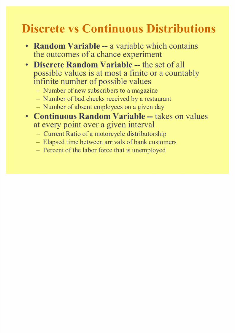
Discrete vs Continuous Distributions
Random Variable -- a variable which containsthe outcomes of a chance experiment
Discrete Random Variable -- the set of all possible values is at most a finite or a countably
infinite number of possible values ± Number of new subscribers to a magazine
± Number of bad checks received by a restaurant
± Number of absent employees on a given day
Continuous Random Variable -- takes on values
at every point over a given interval ± Current Ratio of a motorcycle distributorship
± Elapsed time between arrivals of bank customers
± Percent of the labor force that is unemployed

8/3/2019 01.Discrete Prob. Distribution
http://slidepdf.com/reader/full/01discrete-prob-distribution 3/36
Some Special Distributions
Discrete ± binomial ± Poisson ±
hyp
ergeometric Continuous ± normal ± uniform ± exponential
± t ± chi-square ± F

8/3/2019 01.Discrete Prob. Distribution
http://slidepdf.com/reader/full/01discrete-prob-distribution 4/36
Discrete Distribution -- Example
0
1
2
34
5
0.37
0.31
0.18
0.090.04
0.01
Number of Crises
Probability
Distribution of DailyCrises
0
0.1
0.2
0.3
0.40.5
0 1 2 3 4 5
P
ro
b
a
b
i
l
it
yNumber of Crises

8/3/2019 01.Discrete Prob. Distribution
http://slidepdf.com/reader/full/01discrete-prob-distribution 5/36
Requirements for a
Discrete Probability Function Probabilities are between 0 and 1,
inclusively
Total of all probabilities equals 1
0 1e e P X ( ) for all X
P X ( )over all x§ ! 1

8/3/2019 01.Discrete Prob. Distribution
http://slidepdf.com/reader/full/01discrete-prob-distribution 6/36
Requirements for a Discrete
Probability Function -- ExamplesX P(X)
-10
1
2
3
.1.2
.4
.2
.11.0
X P(X)
-1
0
1
2
3
-.1
.3
.4
.3
.11.0
X P(X)
-10
1
2
3
.1.3
.4
.3
.11.2

8/3/2019 01.Discrete Prob. Distribution
http://slidepdf.com/reader/full/01discrete-prob-distribution 7/36
Mean of a Discrete Distribution
Q ! ! § E X X P X ( )
X
-1
0
12
3
P(X)
.1
.2
.4
.2
.1
-.1
.0
.4
.4
.3
1.0
X P X ( )

8/3/2019 01.Discrete Prob. Distribution
http://slidepdf.com/reader/full/01discrete-prob-distribution 8/36
Variance and Standard Deviation
of a Discrete Distribution
2.1)(22
!! § X P X QW W W! ! $2
12 110. .
X
-1
0
12
3
P(X)
.1
.2
.4
.2
.1
-2
-1
01
2
X Q
4
1
01
4
.4
.2
.0
.2
.4
1.2
)(2
Q
X 2
( ) ( ) X P X Q

8/3/2019 01.Discrete Prob. Distribution
http://slidepdf.com/reader/full/01discrete-prob-distribution 9/36
Mean of the Crises Data Example
Q ! ! !§ E X X P X ( ) .115
X P(X) XyP(X)
0 .37 .00
1 .31 .31
2 .18 .36
3 .09 .27
4 .04 .16
5 .01 .05
1.15
0
0.1
0.20.3
0.4
0.5
0 1 2 3 4 5
P
r
o
b
a
b
i
l
i
t
y
Number of Crises
An executive is considering out of town business travel for a given
Friday. She recognizes that at least one crises could occur on the day
that she is gone and she is concerned about the possibilities. Table
shows a discrete distribution that contains the number of crisis that
could occur during the day she is gone and the probability that each
number will occur.

8/3/2019 01.Discrete Prob. Distribution
http://slidepdf.com/reader/full/01discrete-prob-distribution 10/36
Variance and Standard Deviation
of Crises Data Example
22
141W Q! !§ X P X ( ) . W W! ! !2
141 119. .
X P(X) (X-Q) (X-Q)2 (X-Q)2yP(X)
0 .37 -1.15 1.32 .49
1 .31 -0.15 0.02 .01
2 .18 0.85 0.72 .13
3 .09 1.85 3.42 .31
4 .04 2.85 8.12 .32
5 .01 3.85 14.82 .15
1.41

8/3/2019 01.Discrete Prob. Distribution
http://slidepdf.com/reader/full/01discrete-prob-distribution 11/36
Binomial Distribution
Experiment involves n identical trials Each trial has exactly two possible outcomes: successand failure
Each trial is independent of the previous trials
p is the probability of a success on any one trial
q = (1- p) is the probability of a failure on any onetrial
p and q are constant throughout the experiment
X is the number of successes in the n trials
8/3/2019 01.Discrete Prob. Distribution
http://slidepdf.com/reader/full/01discrete-prob-distribution 12/36
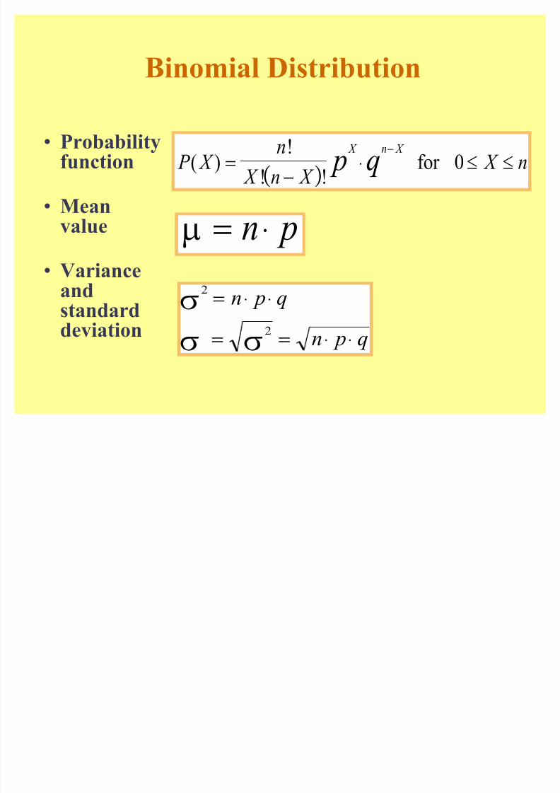
Binomial Distribution
Probabilityfunction
Meanvalue
Variance
andstandarddeviation
P X
n
X n X X n
X n X
p q( )!
! !!
e e
for 0
Q ! n p
2
2
W
W W
!
! !
n p q
n p q
8/3/2019 01.Discrete Prob. Distribution
http://slidepdf.com/reader/full/01discrete-prob-distribution 13/36
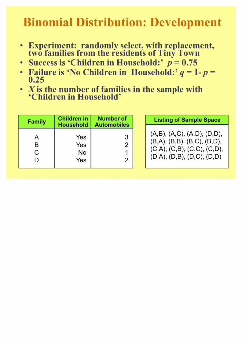
Binomial Distribution: Development
Experiment: randomly select, with replacement,two families from the residents of Tiny Town
Success is µChildren in Household:¶ p = 0.75 Failure is µNo Children in Household:¶ q = 1- p =
0.25 X is the number of families in the sample with
µChildren in Household¶
FamilyChildren in
Household
Number of
Automobiles
A
B
C
D
Yes
Yes
No
Yes
3
2
1
2
Listing of Sample Space
(A,B), (A,C), (A,D), (D,D),
(B,A), (B,B), (B,C), (B,D),
(C,A), (C,B), (C,C), (C,D),
(D,A), (D,B), (D,C), (D,D)

8/3/2019 01.Discrete Prob. Distribution
http://slidepdf.com/reader/full/01discrete-prob-distribution 14/36
Binomial Distribution: Development
Continued Families A, B, and D have
children in the household;family C does not
Success is µChildren inHousehold:¶ p = 0.75
Failure is µNo Children inHousehold:¶ q = 1- p = 0.25
X is the number of families
in the sample withµChildren in Household¶
(A,B),
(A,C),
(A,D),
(D,D),
(B,A),
(B,B),
(B,C),
(B,D),
(C,A),
(C,B),
(C,C),
(C,D),
(D,A),
(D,B),
(D,C),
(D,D)
Listing of SampleSpace
2
1
2
2
2
2
1
2
1
1
0
1
2
2
1
2
X
1/16
1/16
1/16
1/16
1/16
1/16
1/16
1/16
1/16
1/16
1/16
1/16
1/16
1/16
1/16
1/16
P(outcome)
8/3/2019 01.Discrete Prob. Distribution
http://slidepdf.com/reader/full/01discrete-prob-distribution 15/36
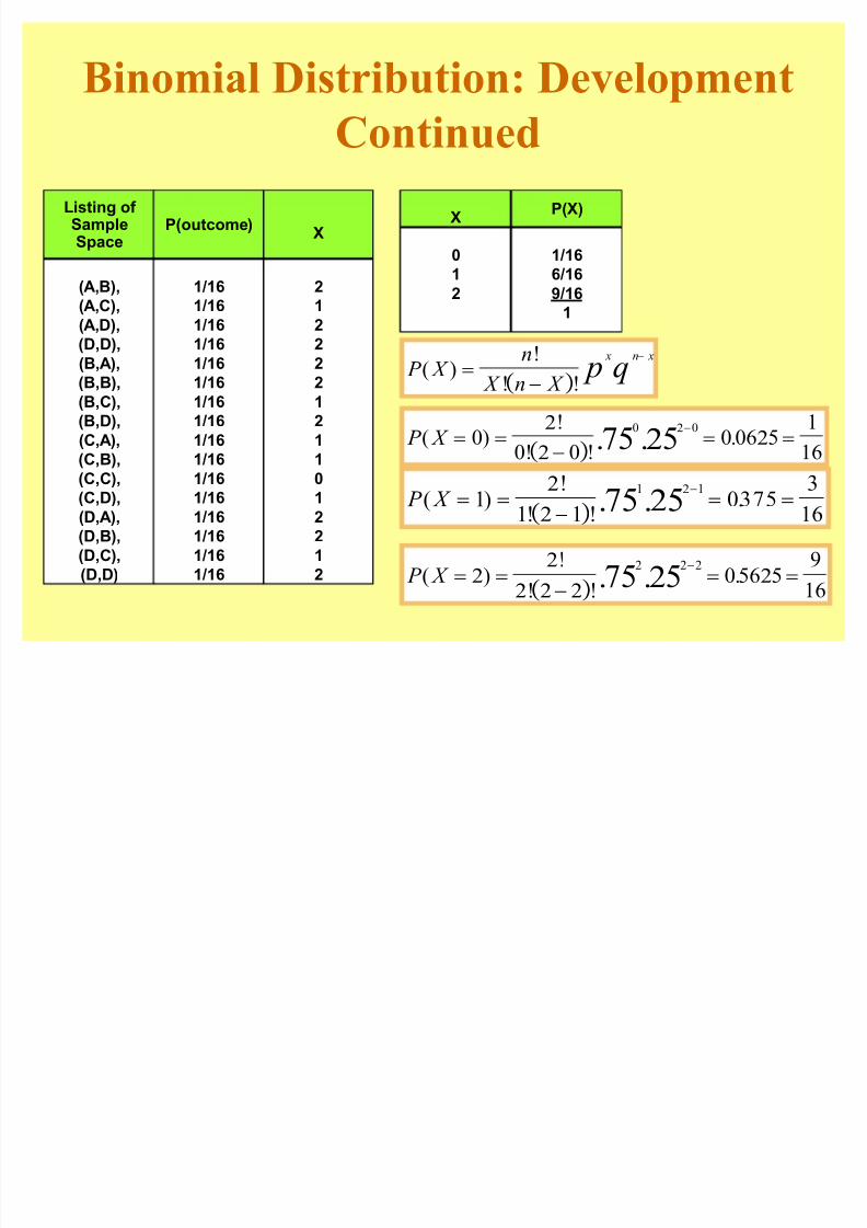
Binomial Distribution: Development
Continued
(A,B),
(A,C),(A,D),
(D,D),
(B,A),
(B,B),
(B,C),
(B,D),
(C,A),
(C,B),(C,C),
(C,D),
(D,A),
(D,B),
(D,C),
(D,D)
Listing of SampleSpace
2
12
2
2
2
1
2
1
10
1
2
2
1
2
X
1/16
1/161/16
1/16
1/16
1/16
1/16
1/16
1/16
1/161/16
1/16
1/16
1/16
1/16
1/16
P(outcome) X
0
1
2
1/16
6/16
9/16
1
P(X)
P X
n
X n X
x n x
p q( )!
! !!
P X ( )!
!
.. .! !
! !
02
0! 2 0
0 06251
16
0 2 0
75 25
P X ( )
!
! !.. .! !
! !
1
2
1 2 10375
3
16
1 2 1
75 25
P X ( )
!
! !.. .! !
! !
22
2 2 20 5625
9
16
2 2 2
75 25

8/3/2019 01.Discrete Prob. Distribution
http://slidepdf.com/reader/full/01discrete-prob-distribution 16/36
Binomial Distribution: Development
Continued Families A, B, and Dhave children in thehousehold; family Cdoes not
Success is µChildren inHousehold:¶ p = 0.75
Failure is µNo Childrenin Household:¶ q = 1- p = 0.25
X is the number of families in the samplewith µChildren inHousehold¶
XPossible
Sequences
0
1
1
2
(F,F)
(S,F)
(F,S)
(S,S)
P(sequence)
(. )(. ) (. )25 25225!
(. )(. )25 75
(. )(. )75 25
(. )(. ) (. )75 75275!

8/3/2019 01.Discrete Prob. Distribution
http://slidepdf.com/reader/full/01discrete-prob-distribution 17/36
Binomial Distribution: Development
ContinuedX
PossibleSequences
0
1
1
2
(F,F)
(S,F)
(F,S)
(S,S)
P(sequence)
(. )(. ) (. )25 25225!
(. )(. )25 75
(. )(. )75 25
(. )(. ) (. )75 75275!
X
0
1
2
P(X)
(. )(. )25 752 =0.375
(. )(. ) (. )75 75275! =0.5625
(. )(. ) (. )25 25225! =0.0625
P X
n
X n X
x n x
p q( )!
! !!
P X ( ) !
!.. .! !
!
02
0! 2 00 0625
0 2 0
75 25 P X ( ) !
! !.. .! !
!
1 2
1 2 10 375
1 2 1
75 25
P X ( )
!
! !.. .! !
!
2
2
2 2 20 5625
2 2 2
75 25

8/3/2019 01.Discrete Prob. Distribution
http://slidepdf.com/reader/full/01discrete-prob-distribution 18/36
Binomial Distribution: Demonstration Problem
n
pq
P X P X P X P X
!
!
!
e ! ! ! !
! !
20
0694
2 0 1 2
2901 3703 2246 8850
.
.
( ) ( ) ( ) ( )
. . . .
P X ( )
)!
( )( )(. ) .. .! !
! !
020!
0!(20 0
1 1 2901 29010 20 0
06 94
P X ( )!( )!
( )(. )(. ) .. .! !
! !
120!
1 20 120 06 3086 3703
1 20 1
06 94
P X ( )
!( )!
( )(. )(. ) .. .! !
! !
220!
2 20 2
190 0036 3283 22462 20 2
06 94
According to the U.S. census Bureau, approximately 6% of all
workers in Jacson, Mississippi, are unemployed. In conducting a random telephone survey in Jacson, what is the probability
of getting two or fewer unemployed workers in a sample of 20?

8/3/2019 01.Discrete Prob. Distribution
http://slidepdf.com/reader/full/01discrete-prob-distribution 19/36
BinomialTable
n = 20 PROBABILITY
X 0.1 0.2 0.3 0.4 0.5 0.6 0.7 0.8 0.9
0 0.122 0.012 0.001 0.000 0.000 0.000 0.000 0.000 0.0001 0.270 0.058 0.007 0.000 0.000 0.000 0.000 0.000 0.000
2 0.285 0.137 0.028 0.003 0.000 0.000 0.000 0.000 0.000
3 0.190 0.205 0.072 0.012 0.001 0.000 0.000 0.000 0.000
4 0.090 0.218 0.130 0.035 0.005 0.000 0.000 0.000 0.000
5 0.032 0.175 0.179 0.075 0.015 0.001 0.000 0.000 0.000
6 0.009 0.109 0.192 0.124 0.037 0.005 0.000 0.000 0.000
7 0.002 0.055 0.164 0.166 0.074 0.015 0.001 0.000 0.000
8 0.000 0.022 0.114 0.180 0.120 0.035 0.004 0.000 0.000
9 0.000 0.007 0.065 0.160 0.160 0.071 0.012 0.000 0.000
10 0.000 0.002 0.031 0.117 0.176 0.117 0.031 0.002 0.000
11 0.000 0.000 0.012 0.071 0.160 0.160 0.065 0.007 0.000
12 0.000 0.000 0.004 0.035 0.120 0.180 0.114 0.022 0.000
13 0.000 0.000 0.001 0.015 0.074 0.166 0.164 0.055 0.002
14 0.000 0.000 0.000 0.005 0.037 0.124 0.192 0.109 0.009
15 0.000 0.000 0.000 0.001 0.015 0.075 0.179 0.175 0.032
16 0.000 0.000 0.000 0.000 0.005 0.035 0.130 0.218 0.090
17 0.000 0.000 0.000 0.000 0.001 0.012 0.072 0.205 0.19018 0.000 0.000 0.000 0.000 0.000 0.003 0.028 0.137 0.285
19 0.000 0.000 0.000 0.000 0.000 0.000 0.007 0.058 0.270
20 0.000 0.000 0.000 0.000 0.000 0.000 0.001 0.012 0.122

8/3/2019 01.Discrete Prob. Distribution
http://slidepdf.com/reader/full/01discrete-prob-distribution 20/36
Using the
Binomial Table
Demonstration
Problem
n = 20 PROBABILITY
X 0.1 0.2 0.3 0.4
0 0.122 0.012 0.001 0.000
1 0.270 0.058 0.007 0.000
2 0.285 0.137 0.028 0.003
3 0.190 0.205 0.072 0.012
4 0.090 0.218 0.130 0.035
5 0.032 0.175 0.179 0.075
6 0.009 0.109 0.192 0.124
7 0.002 0.055 0.164 0.166
8 0.000 0.022 0.114 0.180
9 0.000 0.007 0.065 0.160
10 0.000 0.002 0.031 0.117
11 0.000 0.000 0.012 0.071
12 0.000 0.000 0.004 0.035
13 0.000 0.000 0.001 0.015
14 0.000 0.000 0.000 0.005
15 0.000 0.000 0.000 0.001
16 0.000 0.000 0.000 0.00017 0.000 0.000 0.000 0.000
18 0.000 0.000 0.000 0.000
19 0.000 0.000 0.000 0.000
20 0.000 0.000 0.000 0.000
1171.0)10(
40.
20
60.40.1010
1020 !!!
!
!
C X P
p
n

8/3/2019 01.Discrete Prob. Distribution
http://slidepdf.com/reader/full/01discrete-prob-distribution 21/36
Binomial Distribution using Table:
Demonstration Problem
n
p
q
P X P X P X P X
!
!
!
e ! ! ! !
! !
20
06
94
2 0 1 2
2901 3703 2246 8850
.
.
( ) ( ) ( ) ( )
. . . .
P X P X ( ) ( ) . ." ! e ! !2 1 2 1 8850 1150
Q ! ! !n p ( )(. ) .20 06 1 202
2
20 06 94 1 128
1 128 1 062
W
W W
! ! !
! ! !
n p q ( )(. )(. ) .
. .
n = 20 PROBABILITY
X 0.05 0.06 0.07
0 0.3585 0.2901 0.2342
1 0.3774 0.3703 0.3526
2 0.1887 0.2246 0.2521
3 0.0596 0.0860 0.1139
4 0.0133 0.0233 0.0364
5 0.0022 0.0048 0.0088
6 0.0003 0.0008 0.0017
7 0.0000 0.0001 0.0002
8 0.0000 0.0000 0.0000
« « «
20 0.0000 0.0000 0.0000
«
According to a published data, Oreos control about 10% of themarket for cookie brands. Suppose 20 purchasers of cookies are
selected randomly from the population. What is the probability
that fewer than four purchasers choose Oreos?
8/3/2019 01.Discrete Prob. Distribution
http://slidepdf.com/reader/full/01discrete-prob-distribution 22/36
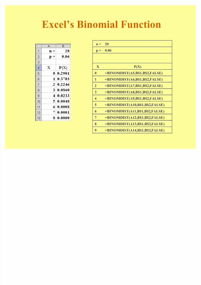
Excel¶s Binomial Function
n = 20
p = 0.06
X P(X)
0 =BINOMDIST(A5,B$1,B$2,FALSE)
1 =BINOMDIST(A6,B$1,B$2,FALSE)
2 =BINOMDIST(A7,B$1,B$2,FALSE)
3 =BINOMDIST(A8,B$1,B$2,FALSE)
4 =BINOMDIST(A9,B$1,B$2,FALSE)
5 =BINOMDIST(A10,B$1,B$2,FALSE)6 =BINOMDIST(A11,B$1,B$2,FALSE)
7 =BINOMDIST(A12,B$1,B$2,FALSE)
8 =BINOMDIST(A13,B$1,B$2,FALSE)
9 =BINOMDIST(A14,B$1,B$2,FALSE)

8/3/2019 01.Discrete Prob. Distribution
http://slidepdf.com/reader/full/01discrete-prob-distribution 23/36
Graphs of Selected Binomial Distributions
n = 4 PROBABILITY
X 0.1 0.5 0.9
0 0.656 0.063 0.000
1 0.292 0.250 0.004
2 0.049 0.375 0.049
3 0.004 0.250 0.292
4 0.000 0.063 0.656
P = 0.1
0.000
0.100
0.200
0.300
0.4000.500
0.600
0.700
0.800
0.900
1.000
0 1 2 3 4X
P ( X )
P = 0.5
0.000
0.100
0.200
0.300
0.400
0.500
0.600
0.700
0.800
0.9001.000
0 1 2 3 4X
P ( X )
P = 0.9
0.000
0.100
0.200
0.300
0.4000.500
0.600
0.700
0.800
0.900
1.000
0 1 2 3 4X
P ( X )

8/3/2019 01.Discrete Prob. Distribution
http://slidepdf.com/reader/full/01discrete-prob-distribution 24/36
Poisson Distribution
A discrete distribution Describes discrete occurrences over a
continuum or interval
Describes rare events Each occurrence is independent any other
occurrences.
The number of occurrences in each interval
can vary from zero to infinity.
The expected number of occurrences musthold constant throughout the experiment.

8/3/2019 01.Discrete Prob. Distribution
http://slidepdf.com/reader/full/01discrete-prob-distribution 25/36
Poisson Distribution: Applications
Arrivals at queuing systems ± airports -- people, airplanes, baggage ± banks -- people, automobiles, loan applications
Defects in manufactured goods ± number of defects per 1,000 feet of extruded
copper wire ± number of blemishes per square foot of painted
surface ± number of errors per typed page

8/3/2019 01.Discrete Prob. Distribution
http://slidepdf.com/reader/full/01discrete-prob-distribution 26/36
Poisson Distribution
Probability function
P X
X
X
where
long run average
e
X
e( )!
, , , , ...
:
. . ..
! !
!
!
PP
P
for
(the base of natural logarithms)
0 1 2 3
2
7182
82
P
Mean valueMean value
P
Standard deviationStandard deviation VarianceVariance
P

8/3/2019 01.Discrete Prob. Distribution
http://slidepdf.com/reader/full/01discrete-prob-distribution 27/36
Bank customers arrive randomly on weekday afternoons at an
average of 3.2 customers every 4 minutes. What is the
probability of getting exactly 10 customers during an 8
minutes interval on a weekday afternoon?
Poisson Distribution: Demonstration
Problem

8/3/2019 01.Discrete Prob. Distribution
http://slidepdf.com/reader/full/01discrete-prob-distribution 28/36
Poisson Distribution: Demonstration
Problem
P
P
P
PP
!
!
3 2
6 4
1010
0 0528
6 4
.
!
!.
.
customers / 4 minutes
X = 10 customers / 8 minutes
Adjusted
= . customers / 8 minutes
P(X) =
( = ) =
X
10
6.4
e
e
X
P X
P
P
P
PP
!
!
3 2
6 4
66
0 1586
6 4
.
!
!.
.
customers / 4 minutes
X = 6 customers / 8 minutes
Adjusted
= . customers / 8 minutes
P(X) =
( = ) =
X
6
6.4
e
e
X
P X

8/3/2019 01.Discrete Prob. Distribution
http://slidepdf.com/reader/full/01discrete-prob-distribution 29/36
Poisson Distribution: Probability Table
X 0.5 1.5 1.6 3.0 3.2 6.4 6.5 7.0 8.0
0 0.6065 0.2231 0.2019 0.0498 0.0408 0.0017 0.0015 0.0009 0.0003
1 0.3033 0.3347 0.3230 0.1494 0.1304 0.0106 0.0098 0.0064 0.0027
2 0.0758 0.2510 0.2584 0.2240 0.2087 0.0340 0.0318 0.0223 0.0107
3 0.0126 0.1255 0.1378 0.2240 0.2226 0.0726 0.0688 0.0521 0.0286
4 0.0016 0.0471 0.0551 0.1680 0.1781 0.1162 0.1118 0.0912 0.0573
5 0.0002 0.0141 0.0176 0.1008 0.1140 0.1487 0.1454 0.1277 0.09166 0.0000 0.0035 0.0047 0.0504 0.0608 0.1586 0.1575 0.1490 0.1221
7 0.0000 0.0008 0.0011 0.0216 0.0278 0.1450 0.1462 0.1490 0.1396
8 0.0000 0.0001 0.0002 0.0081 0.0111 0.1160 0.1188 0.1304 0.1396
9 0.0000 0.0000 0.0000 0.0027 0.0040 0.0825 0.0858 0.1014 0.1241
10 0.0000 0.0000 0.0000 0.0008 0.0013 0.0528 0.0558 0.0710 0.0993
11 0.0000 0.0000 0.0000 0.0002 0.0004 0.0307 0.0330 0.0452 0.0722
12 0.0000 0.0000 0.0000 0.0001 0.0001 0.0164 0.0179 0.0263 0.0481
13 0.0000 0.0000 0.0000 0.0000 0.0000 0.0081 0.0089 0.0142 0.0296
14 0.0000 0.0000 0.0000 0.0000 0.0000 0.0037 0.0041 0.0071 0.0169
15 0.0000 0.0000 0.0000 0.0000 0.0000 0.0016 0.0018 0.0033 0.0090
16 0.0000 0.0000 0.0000 0.0000 0.0000 0.0006 0.0007 0.0014 0.0045
17 0.0000 0.0000 0.0000 0.0000 0.0000 0.0002 0.0003 0.0006 0.0021
18 0.0000 0.0000 0.0000 0.0000 0.0000 0.0001 0.0001 0.0002 0.0009
P

8/3/2019 01.Discrete Prob. Distribution
http://slidepdf.com/reader/full/01discrete-prob-distribution 30/36
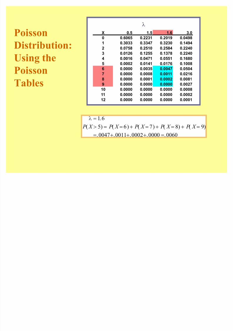
Poisson Distribution: Using the
Poisson Tables
X 0.5 1.5 1.6 3.0
0 0.6065 0.2231 0.2019 0.0498
1 0.3033 0.3347 0.3230 0.1494
2 0.0758 0.2510 0.2584 0.2240
3 0.0126 0.1255 0.1378 0.2240
4 0.0016 0.0471 0.0551 0.1680
5 0.0002 0.0141 0.0176 0.1008
6 0.0000 0.0035 0.0047 0.0504
7 0.0000 0.0008 0.0011 0.0216
8 0.0000 0.0001 0.0002 0.0081
9 0.0000 0.0000 0.0000 0.0027
10 0.0000 0.0000 0.0000 0.0008
11 0.0000 0.0000 0.0000 0.0002
12 0.0000 0.0000 0.0000 0.0001
P
P !
! !
1 6
4 0 0551
.
( ) . P X
8/3/2019 01.Discrete Prob. Distribution
http://slidepdf.com/reader/full/01discrete-prob-distribution 31/36
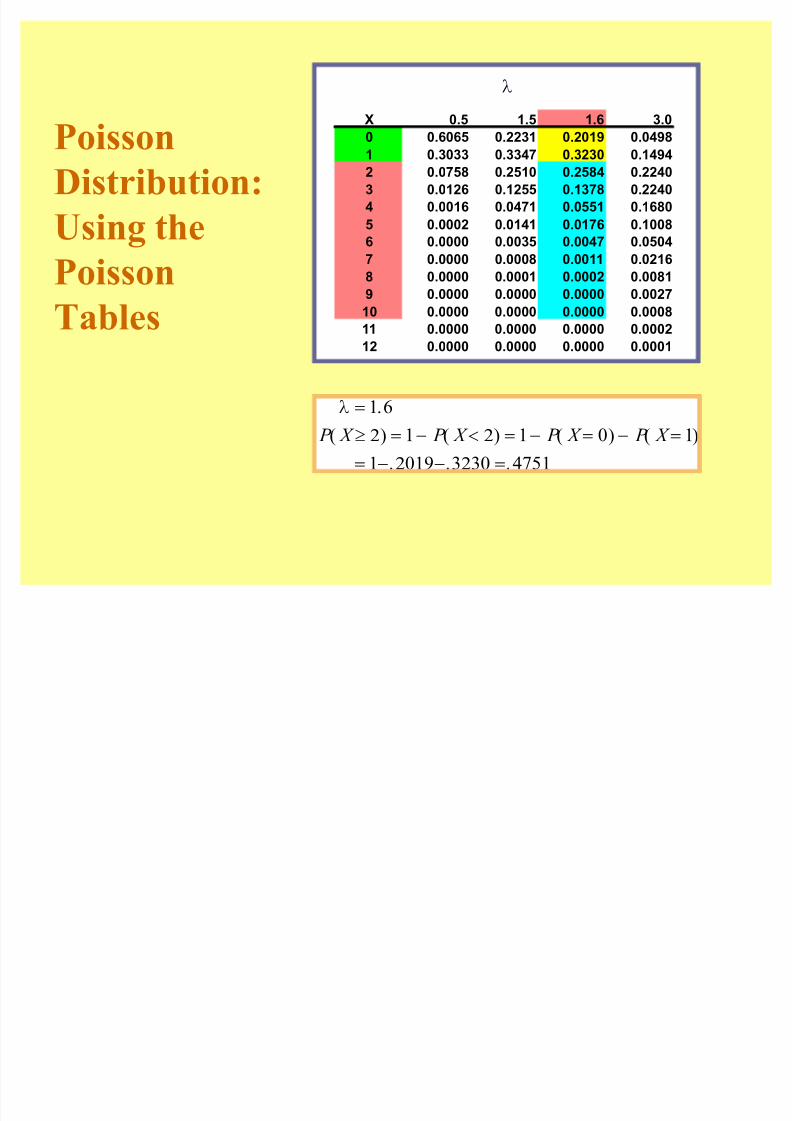
Poisson
Distribution:
Using the
Poisson
Tables
P
X 0.5 1.5 1.6 3.0
0 0.6065 0.2231 0.2019 0.0498
1 0.3033 0.3347 0.3230 0.14942 0.0758 0.2510 0.2584 0.2240
3 0.0126 0.1255 0.1378 0.2240
4 0.0016 0.0471 0.0551 0.1680
5 0.0002 0.0141 0.0176 0.1008
6 0.0000 0.0035 0.0047 0.0504
7 0.0000 0.0008 0.0011 0.0216
8 0.0000 0.0001 0.0002 0.0081
9 0.0000 0.0000 0.0000 0.0027
10 0.0000 0.0000 0.0000 0.0008
11 0.0000 0.0000 0.0000 0.0002
12 0.0000 0.0000 0.0000 0.0001
P !
" ! ! ! ! !
! !
1 6
5 6 7 8 9
0047 0011 0002 0000 0060
.
( ) ( ) ( ) ( ) ( )
. . . . .
P X P X P X P X P X
8/3/2019 01.Discrete Prob. Distribution
http://slidepdf.com/reader/full/01discrete-prob-distribution 32/36
PoissonDistribution:
Using the
PoissonTables
P !
u ! ! ! !
! !
1 6
2 1 2 1 0 1
1 2019 3230 4751
.
( ) ( ) ( ) ( )
. . .
P X P X P X P X
P
X 0.5 1.5 1.6 3.0
0 0.6065 0.2231 0.2019 0.04981 0.3033 0.3347 0.3230 0.1494
2 0.0758 0.2510 0.2584 0.2240
3 0.0126 0.1255 0.1378 0.2240
4 0.0016 0.0471 0.0551 0.1680
5 0.0002 0.0141 0.0176 0.1008
6 0.0000 0.0035 0.0047 0.0504
7 0.0000 0.0008 0.0011 0.0216
8 0.0000 0.0001 0.0002 0.00819 0.0000 0.0000 0.0000 0.0027
10 0.0000 0.0000 0.0000 0.0008
11 0.0000 0.0000 0.0000 0.0002
12 0.0000 0.0000 0.0000 0.0001

8/3/2019 01.Discrete Prob. Distribution
http://slidepdf.com/reader/full/01discrete-prob-distribution 33/36
Poisson Distribution: Graphs
0.00
0.05
0.10
0.15
0.20
0.25
0.30
0.35
0 1 2 3 4 5 6 7 8
P ! 1 6.
0.00
0.02
0.04
0.06
0.08
0.10
0.12
0.14
0.16
0 2 4 6 8 10 12 14 16
P ! 6 5.
8/3/2019 01.Discrete Prob. Distribution
http://slidepdf.com/reader/full/01discrete-prob-distribution 34/36
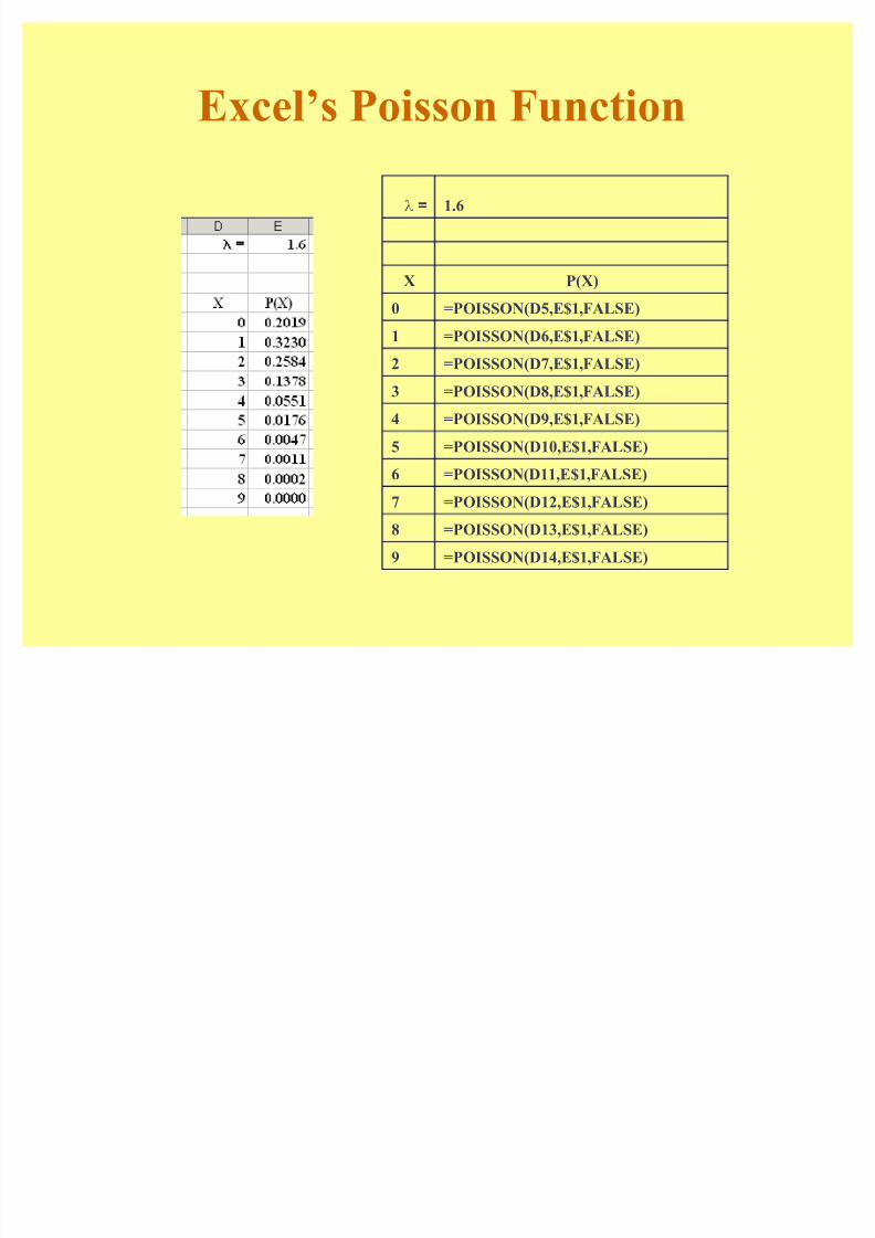
Excel¶s Poisson Function
P = 1.6
X P(X)
0 =POISSON(D5,E$1,FALSE)
1 =POISSON(D6,E$1,FALSE)
2 =POISSON(D7,E$1,FALSE)
3 =POISSON(D8,E$1,FALSE)
4 =POISSON(D9,E$1,FALSE)
5 =POISSON(D10,E$1,FALSE)
6 =POISSON(D11,E$1,FALSE)
7 =POISSON(D12,E$1,FALSE)
8 =POISSON(D13,E$1,FALSE)
9 =POISSON(D14,E$1,FALSE)

8/3/2019 01.Discrete Prob. Distribution
http://slidepdf.com/reader/full/01discrete-prob-distribution 35/36
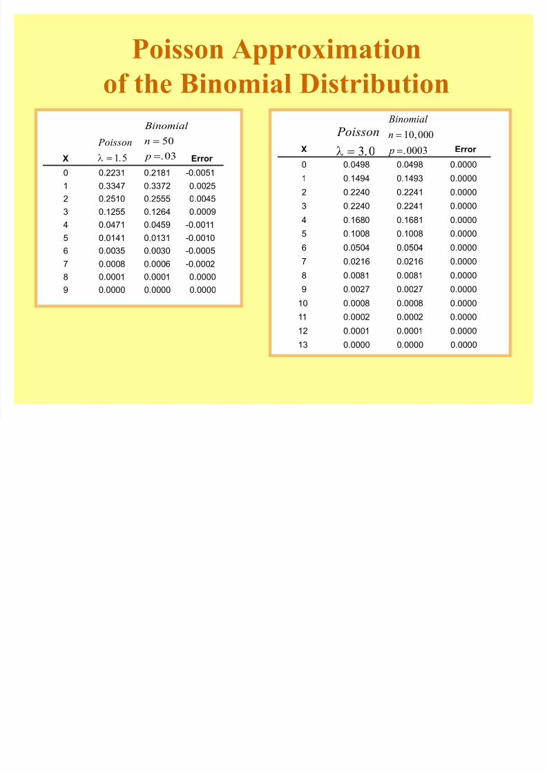
Poisson Approximation
of the Binomial Distribution
Binomial probabilities are difficult tocalculate when n is large.
Under certain conditions binomial
probabilities may be approximated byPoisson probabilities.
Poisson approximation
If and the approximation is acceptable.n n p" e20 7,
Use P ! n p.
8/3/2019 01.Discrete Prob. Distribution
http://slidepdf.com/reader/full/01discrete-prob-distribution 36/36
Poisson Approximation
of the Binomial Distribution
X Error
0 0.2231 0.2181 -0.0051
1 0.3347 0.3372 0.0025
2 0.2510 0.2555 0.0045
3 0.1255 0.1264 0.0009
4 0.0471 0.0459 -0.0011
5 0.0141 0.0131 -0.0010
6 0.0035 0.0030 -0.0005
7 0.0008 0.0006 -0.0002
8 0.0001 0.0001 0.0000
9 0.0000 0.0000 0.0000
P oisson
P ! 1 5.
Binomial
n
p
!
!
50
03.X Error
0 0.0498 0.0498 0.0000
1 0.1494 0.1493 0.0000
2 0.2240 0.2241 0.0000
3 0.2240 0.2241 0.0000
4 0.1680 0.1681 0.0000
5 0.1008 0.1008 0.0000
6 0.0504 0.0504 0.0000
7 0.0216 0.0216 0.0000
8 0.0081 0.0081 0.0000
9 0.0027 0.0027 0.0000
10 0.0008 0.0008 0.0000
11 0.0002 0.0002 0.0000
12 0.0001 0.0001 0.0000
13 0.0000 0.0000 0.0000
P oisson
P ! 3 0.
Binomial
n
p
!
!
10 000
0003
,
.