University of Rhode IslandDigitalCommons@URI

Nonequilibrium Statistical Physics Physics Course Materials

2015

08. Brownian MotionGerhard MüllerUniversity of Rhode Island, gmuller@uri.edu

Creative Commons License

This work is licensed under a Creative Commons Attribution-Noncommercial-Share Alike 4.0 License.

Follow this and additional works at: http://digitalcommons.uri.edu/nonequilibrium_statistical_physics

Part of the Physics Commons

AbstractPart eight of course materials for Nonequilibrium Statistical Physics (Physics 626), taught byGerhard Müller at the University of Rhode Island. Entries listed in the table of contents, but notshown in the document, exist only in handwritten form. Documents will be updated periodically asmore entries become presentable.Updated with version 2 on 5/3/2016.

This Course Material is brought to you for free and open access by the Physics Course Materials at DigitalCommons@URI. It has been accepted forinclusion in Nonequilibrium Statistical Physics by an authorized administrator of DigitalCommons@URI. For more information, please contactdigitalcommons@etal.uri.edu.

Recommended CitationMüller, Gerhard, "08. Brownian Motion" (2015). Nonequilibrium Statistical Physics. Paper 8.http://digitalcommons.uri.edu/nonequilibrium_statistical_physics/8

Contents of this Document [ntc8]

8. Brownian Motion

• Early Landmarks [nln63]

• Relevant time scales (collisions, relaxation, observations) [nln64]

• Einstein’s theory [nln65]

• Diffusion equation analyzed [nln73]

• Release of Brownian particle from box confinement [nex128]

• Smoluchowski equation [nln66]

• Einstein’s fluctuation-dissipation relation [nln67]

• Smoluchowski vs Fokker-Planck [nln68]

• Fourier’s law for heat conduction [nln69]

• Thermal diffusivity [nex117

• Shot noise [nln70]

• Campbell’s theorem [nex37]

• Critically damped ballistic galvanometer [nex70]

• Langevin’s theory [nln71]

• White noise

• Brownian motion and Gaussian white noise [nln20]

• Wiener process [nsl4]

• Autocorrelation function of Wiener process [nex54]

• Attenuation without memory [nln21]

• Formal solution of Langevin equation [nex53]

• Velocity correlation function of Brownian particle I [nex55]

• Mean-square displacement of Brownian particle [nex56], [nex57], [nex118]

• Ergodicity [nln13]

• Intensity spectrum and spectral density (Wiener-Khintchine theorem)[nln14]

• Fourier analysis of Langevin equation

• Velocity correlation function of Bownian particle II [nex119]

• Generalized Langevin equation [nln72]

• Attenuation with memory [nln22]

• Velocity correlation function of Brownian particle III [nex120]

• Brownian harmonic oscillator [nln75]

• Brownian harmonic oscillator VII: equivalent specifications [nex129]

• Brownian harmonic oscillator I: Fourier analysis [nex121]

• Brownian harmonic oscillator II: position correlation function [nex122]

• Brownian harmonic oscillator III: contour integrals [nex123]

• Brownian harmonic oscillator IV: velocity correlations [nex58]

• Brownian harmonic oscillator V: formal solution for velocity [nex59]

• Brownian harmonic oscillator VI: nonequilibrium correlations [nex60]

• Langevin dynamics from microscopic model [nln74]

• Brownian motion: levels of contraction and modes of description [nln23]

Brownian Motion [nln63]

Early experimental evidence for atomic structure of matter. Historically im-portant in dispute between ’atomicists’ and ’energeticists’ in late 19th cen-tury.

Brown 1828:Observation of perpetual, irregular motion of pollen grains suspended in wa-ter. The particles visible under a microscope (pollen) are small enough tobe manifestly knocked around by even smaller particles that are not directlyvisible (molecules).

Einstein, Smoluchowski 1905:Correct interpretation of Brownian motion as caused by collisions with themolecules of a liquid. Theoretical framework of thermal fluctuations groundedin the assumption that matter has a molecular structure and with aspectsthat are experimentally testable.

Perrin 1908:Systematic observations of Brownian motion combined with quantitativeanalysis. Confirmation of Einstein’s predictions. Experimental determina-tion of Avogadro’s number.

Langevin 1908:Confirmation of Einstein’s results via different approach. Langevin’s ap-proach provided more detailed (less contracted) description of Brownian mo-tion. Langevin equation proven to be generalizable. Foundation of generaltheory of fluctuations rooted in microscopic dynamics.

Relevant Time Scales [nln64]

Conceptually, it is useful to distinguish between heavy and light Brownianparticles. For the most part, only Brownian particles that are heavy com-pared to the fluid molecules are large enough to be visible under a microscope.

Time scales relevant in the observation and analysis of Brownian particles:

• ∆τC: time between collisions,

• ∆τR: relaxation time,

• ∆τO: time between observations.

Heavy Brownian particles: ∆τC ∆τR ∆τO.

Light Brownian particles: ∆τC ' ∆τR ∆τO.

Einstein’s Theory [nln65]

Theory operates on time scale dt, where ∆τR ¿ dt ¿ ∆τO.Focus on one space coordinate: x.Local number density of Brownian particles: n(x, t).Brownian particles experience shift of size s in time dt.Probability distribution of shifts: P (s).Successive shifts are assumed to be statistically independent.Assumption justified by choice of time scale: ∆τR ¿ dt.

Effect of shifts on profile of number density:

n(x, t + dt) =

∫ +∞

−∞ds P (s)n(x + s, t).

Expansion of n(x, t) in space and in time:

n(x + s, t) = n(x, t) + s∂

∂xn(x, t) +

1

2s2 ∂2

∂x2n(x, t) + · · · ,

n(x, t + dt) = n(x, t) + dt∂

∂tn(x, t) + · · ·

Integrals (normalization, reflection symmetry, diffusion coefficient):∫ +∞

−∞ds P (s) = 1,

∫ +∞

−∞ds sP (s) = 0,

1

2

∫ +∞

−∞ds s2P (s)

.= Ddt.

Substitution of expansions with these integrals yields diffusion equation:

∂

∂tn(x, t) = D

∂2

∂x2n(x, t).

Solution with initial condition n(x, 0) = Nδ(x− x0) and no boundaries:

n(x, t) =N√4πDt

exp

(−(x− x0)

2

4Dt

),

No drift: 〈〈x〉〉 = 0.

Diffusive mean-square displacement: 〈〈x2〉〉 = 2Dt.

Diffusion Equation Analyzed [nln73]

Here we present two simple and closely related methods of analyzing thediffusion equation,

∂

∂tρ(x, t) = D

∂2

∂x2ρ(x, t), (1)

in one dimension and with no boundary constraints.

Fourier transform:

Ansatz for plane-wave solution: ρ(x, t)k = ρk(t) eikx.

Substitution of ansatz into PDE (1) yields ODE for Fourier amplitude ρk(t),which is readily solved:

d

dtρk(t) = −Dk2ρk(t) ⇒ ρk(t) = ρk(0) e−Dk2t.

Initial Fourier amplitudes from initial distribution:

ρk(0) =

∫ +∞

−∞dx e−ikxρ(x, 0). (2)

Time-dependence of distribution as superposition of plane-wave solutions:

ρ(x, t) =

∫ +∞

−∞

dk

2πeikxρk(0) e−Dk2t. (3)

Green’s function:

Green’s function G(x, t) describes time evolution of point source at x = 0:

G(x, 0) = δ(x) ⇒ Gk(0).=

∫ +∞

−∞dx e−ikxG(x, 0) = 1 ⇒ Gk(t) = e−Dk2t.

⇒ G(x, t) =

∫ +∞

−∞

dk

2πeikx−Dk2t =

1√4πDt

e−x2/4Dt. (4)

Superposition of point-source solutions in the form of a convolution integral:

ρ(x, t) =

∫ +∞

−∞dx′ρ(x′, 0)G(x− x′, t). (5)

[nex128] Release of Brownian particle from box confinement

Consider a physical ensemble of Brownian particles uniformly distributed inside a one-dimensionalbox. The initial density is

ρ(x, 0) =1

2θ(1− |x|

),

where θ(x) is the step function. At time t = 0 the particles are released to diffuse left and right.Use the two methods presented in [nln73] to calculate the analytic solution,

ρ(x, t) =1

4

[erf

(x+ 1√

4Dt

)− erf

(x− 1√

4Dt

)],

of the diffusion equation, where the error function is defined as follows:

erf(x).=

2√π

∫ x

0

du e−u2

.

(a) In the Fourier analysis of [nln73] first calculate the initial Fourier amplitudes via (2) and thenuse the result in the integration (3).(b) In the Green’s function analysis of [nln73] perform the involution integral (5) with the point-source solution (4) and the initial rectangular initial distribution pertaining to this application.(c) Plot ρ(x, t) versus x for −3 ≤ x ≤ +3 and Dt = 0, 0.04, 0.2, 1, 5.

Solution:

Smoluchowski Equation [nln66]

Einstein’s result derived from different starting point.

Two laws relating number density and flux of Brownian particles:

(a) Conservation law:∂

∂tn(x, t) = − ∂

∂xj(x, t) (continuity equation);

local change in density due to net flux from or to vicinity.

(b) Constitutive law: j(x, t) = −D ∂

∂xn(x, t) (Fick’s law);

flux driven by gradient in density.

Combination of (a) and (b) yields diffusion equation for density:

∂

∂tn(x, t) = D

∂2

∂x2n(x, t). (1)

Solution of (1) yields flux via (b).

Extension to include drift.

Brownian particles subject to external force Fext(x, t).

Resulting drift velocity v, averaged over time scale dt identified in [nln65],produces drag force Fdrag = −γv due to front/rear asymmetry of collisions.

Damping constant: γ; mobility: γ−1.

Drift contribution to flux j(x, t) has general form n(x, t)v(x, t).

On time scale dt of [nln65], forces are balanced: Fext + Fdrag = 0.

Drift velocity has reached terminal value: vT = −Fext/γ.

(c) Extended constitutive law: j(x, t) = −D ∂

∂xn(x, t) + γ−1Fext(x, t)n(x, t).

Substitution of (c) into (a) yields Smoluchowski equation:

∂

∂tn(x, t) = D

∂2

∂x2n(x, t) − γ−1 ∂

∂x

[n(x, t)Fext(x, t)

]. (2)

The two terms on the rhs represent diffusion and drift, respectively.

Einstein’s Fluctuation-Dissipation Relation [nln67]

Consider a colloid of volume V suspended in a fluid.Excess mass: m = V (ρcoll − ρfluid).External (gravitational) force directed vertically down: Fext = −mg.

Smoluchowski equation [nln66]:

∂

∂tn(z, t) = D

∂2

∂z2n(z, t) + γ−1 ∂

∂z

[n(z, t)mg

].

Stationary solution: ∂n/∂t = 0 ⇒ n = ns(z).

⇒ d

dz

[D

dns

dz+

mg

γns

]= 0; ns(∞) = 0,

dns

dz

∣∣∣∣z=∞

= 0.

⇒ ns(z) = ns(0) exp

(−mg

γDz

).

Comparison with law of atmospheres (thermal equilibrium state) [tex150],

neq(z) = neq(0) exp

(− mg

kBTz

),

implies

D =kBT

γ(Einstein relation).

This is an example of a relation between a quantity representing fluctuations(D) and a quantity representing dissipation (γ).

The Einstein relation was used to estimate Avogadro’s number NA:

• Colloid in the shape of a solid sphere of radius a.

• Motion in incompressible fluid with viscosity η.

• Stokes’ law for drag force: Fdrag = −6πηav = −γv.

• Damping constant γ = 6πηa (experimentally accessible).

• Diffusion constant D (experimentally accessible).

• Ideal gas constant R = NAkB (experimentally accessible).

• Avogadro’s number: NA =RT

6πηaD.

Smoluchowski vs Fokker-Planck [nln68]

The Smoluchowski equation [nln66] as derived from a conservation law andconstitutive law can be transcribed into a Fokker-Planck equation [nln57] ifdensity and flux of particles are replaced by density and flux of probability.

Here we use generic notation:

• density: ρ(x, t),

• flux: J(x, t),

• diffusivity: D(x),

• mobility: Γ,

• external force: F (x).

Conservation law:∂

∂tρ(x, t) = − ∂

∂xJ(x, t).

Constitutive law: J(x, t) = −D(x)∂

∂xρ(x, t) + ΓF (x)ρ(x, t).

⇒ ∂

∂tρ(x, t) = − ∂

∂x

[ΓF (x)ρ(x, t)

]+

∂

∂x

[D(x)

∂

∂xρ(x, t)

]︸ ︷︷ ︸ .

∂2

∂x2

[D(x)ρ(x, t)

]=

∂

∂x

[D′(x)ρ(x, t)

]+

︷ ︸︸ ︷∂

∂x

[D(x)

∂

∂xρ(x, t)

].

⇒ ∂

∂tρ(x, t) = − ∂

∂x

[(ΓF (x) +D′(x)︸ ︷︷ ︸

A(x)

)ρ(x, t)

]+

∂2

∂x2

[D(x)︸ ︷︷ ︸B(x)

ρ(x, t)].

A(x) and B(x) represent drift and diffusion in the Fokker-Planck equation.

Fourier’s Law for Heat Conduction [nln69]

Heat conduction inside a solid involves three field quantities:

• energy density: ε(x, t),

• heat current: J(x, t),

• local temperature: T (x, t).

Relations between field quantities:

(a) conservation law:∂

∂tε(x, t) = − ∂

∂xJ(x, t) (continuity equation),

(b) constitutive law: J(x, t) = −λ∂

∂xT (x, t) (Fourier’s law),

(c) thermodynamic relation: ε(x, t) = cV T (x, t).

Material constants:

• specific heat: cV ,

• thermal conductivity: λ,

• thermal diffusivity: DT = λ/cV .

Diffusion equation from (a)-(c):

∂

∂tT (x, t) = DT

∂2

∂x2T (x, t).

Applications:

B Temperature profile inside wall [nex117]

[nex117] Thermal diffusivity

A solid wall of very large thickness and lateral extension (assumed to occupy all space at z > 0)is brought into contact with a heat source at its surface (z = 0). The wall is initially in thermalequilibrium at temperature T0. The heat source is kept at the higher temperature T1. The contactis established at time t = 0. Show that the temperature profile inside the wall depends on time asfollows:

T (z) = T0 + (T1 − T0)erfc

(z

2√DT t

),

where DT = λ/cV is the thermal diffusivity, λ the thermal conductvity, and cV the specific heat.Then plot T (z)/T0 versus z for 0 ≤ z ≤ 5, T1/T0 = 3, and DT t = 0.2, 1, 5. Describe the meaning ofthe three curves in relation to each other. The complementary error function is defined as follows:

erfc(x).=

2√π

∫ ∞x

du e−u2

.

Solution:

Shot Noise [nln70]

Electric current in a vacuum tube or solid state device described as a randomsequence of discrete events involving microscopic charge transfer:

I(t) =∑k

F (t− tk).

Assumptions:

• uniform event profile F (t) characteristicof process (e.g. as sketched),

• event times tk randomly distributed,

• average number events per unit time: λ.

Attributes characteristic of Poisson process: [nex25] [nex16]

• probability distribution: P (n, t) = e−λt(λt)n/n!,

• mean and variance: 〈〈n〉〉 = 〈〈n2〉〉 = λt.

Probability that n events have taken place until time t reinterpreted as prob-ability that stochastic variable N(t) assumes value n at time t:

P (n, t) = probN(t) = n.

Sample path of N(t) and its derivative:

N(t) =∑k

θ(t− tk), µ(t).=dN

dt=∑k

δ(t− tk).

Sample path of electric current:

I(t) =∑k

F (t− tk) =

∫ +∞

−∞dt′F (t− t′)µ(t′).

Event profile: F (t) = q e−αtθ(t) with charge q0 = q/α per event.

Electric current: I(t) =

∫ t

−∞dt′q e−α(t−t

′)µ(t′).

Stochastic differential equation:

dI

dt= −αI(t) + qµ(t). (1)

Attributes of Poisson process: 〈〈dN(t)〉〉 = 〈〈[dN(t)]2〉〉 = λdt.

Fluctuation variable: dη(t) = dN(t)− λdt ⇒ 〈dη(t)〉 = 0, 〈[dη(t)]2〉 = λdt.

Average current from (1):1

dI(t) =[λq − αI(t)

]dt+ q dη(t) ⇒ 〈dI(t)〉 =

[λq − α〈I(t)〉

]dt

⇒ d

dt〈I(t)〉 = λq − α〈I(t)〉. (2)

Current fluctuations from (1) and (2):2

dI2.= (I + dI)2 − I2 = 2IdI + (dI)2,

〈dI2〉 = 2⟨I([λq − αI]dt+ qdη

)⟩+⟨(

[λq − αI]dt+ qdη)2⟩

=(2λq〈I〉 − 2α〈I2〉+ λq2

)dt+ O

([dt]2

)⇒ 1

2

d

dt〈I2〉 = λq〈I〉 − α〈I2〉+

1

2λq2. (3)

Steady state:d

dt〈I〉S = 0,

d

dt〈I2〉S = 0:

⇒ 〈I〉S =λq

α, 〈〈I2〉〉S

.= 〈I2〉S − 〈I〉2S =

q2λ

2α. (4)

Applications:

B Campbell processes [nex37]

1Use qµ(t)dt = qdN(t) = qdη(t) + qλdt.2Use 〈I(t)dη(t)〉 = 0.

2

[nex37] Campbell processes.

Consider a stationary stochastic process of the general form Y (t) =∑k F (t− tk), where the times

tk are distributed randomly with an average rate λ of occurrences. Campbell’s theorem then yieldsthe following expressions for the mean value and the autocorrelation function of Y :

〈Y 〉 = λ

∫ ∞−∞

dτ F (τ), 〈〈Y (t)Y (0)〉〉 ≡ 〈Y (t)Y (0)〉 − 〈Y (t)〉〈Y (0)〉 = λ

∫ ∞−∞

dτ F (τ)F (τ + t).

Apply Campbell’s theorem to calculate the average current 〈I〉 and the current autocorrelationfunction 〈〈I(t)I(0)〉〉 for a shot noise process with F (t) = qe−αtθ(t), where θ(t) is the step function.Compare the results with those derived in [nln70] along a somewhat different route.

Solution:

[nex70] Critically damped ballistic galvanometer.

The response of a critically damped ballistic galvanometer to a current pulse at t = 0 is Ψ(t) =cte−γt. Consider the situation where the galvanometer experiences a steady stream of independentrandom current pulses, X(t) =

∑k Ψ(t−tk), where the tk are distributed randomly with an average

rate n of occurrences.(a) Use Campbell’s theorem [nex37] to calculate the average displacement 〈X〉 and the autocorre-lation function 〈〈X(t)X(0)〉〉.(b) Show that the associated spectral density reads

SXX(ω).=

∫ +∞

−∞dt eiωt〈〈X(t)X(0)〉〉 =

nc2

(γ2 + ω2)2.

Solution:

Langevin’s Theory [nln71]

Langevin’s theory of Brownian motion operates on a less contracted levelof description than Einstein’s theory [nln65]. The operational time scale issmall compared to the relaxation time: dt ∆τR. [nln64]. On this timescale inertia matters, implying that velocity cannot change abruptly. Velocityand position variables are kinematically coupled.

The Langevin equation,mx = −γx+ f(t), (1)

is constructed from Newton’s second law with two forces acting:

• drag force: −γx (parametrized by mobility γ−1),

• random force: f(t) (Gaussian white noise/Wiener process).

Since we do not know f(t) explicitly we cannot solve (1) for x(t). However,we know enough about f(t) to solve (1) for 〈x2〉 as a function of time [nex118].

First step: derive the linear, 2nd-order ODE for 〈x2〉,

md2

dt2〈x2〉+ γ

d

dt〈x2〉 = 2kBT, (2)

using

• the white-noise implication that the random force and the position areuncorrelated, 〈xf(t)〉,• the equilibrium implication that the average kinetic energy of the Brow-

nian particle satisfies equipartition, 〈x2〉 = kBT/m.

Second step: Integrate (2) twice using

• initial conditions 〈x2〉0 = 0 and d〈x2〉0/dt = 0,

• Einstein’s fluctuation-dissipation relation D = kBT/γ,

• the fact that (2) is a 1st-order ODE for d〈x2〉/dt.

The result reads

〈x2〉 = 2D

[t− m

γ

(1− e−γt/m

)]. (3)

Within the framework of Langevin’s theory, the relaxation time previouslyidentified [nln64] is

∆τR =m

γ.

This relaxation time separates short-time ballistic regime from a long-timediffusive regime:

• t m

γ: 〈x2〉 ∼ Dγ

mt2 =

kBT

mt2 = 〈v2〉t2,

• t m

γ: 〈x2〉 ∼ 2Dt.

Applications and variations:

B Mean-square displacement of Brownian particle [nex56] [nex57] [nex118]

B Formal solution of Langevin equation [nex53]

B Velocity correlation function of Brownian particle [nex55] [nex119] [nex120]

2

Brownian motion and Gaussian white noise [nln20]

Gaussian white noise: completely factorizing stationary process.

• Pw(y1, t1; y2, t2) = Pw(y1)Pw(y2) if t2 6= t1 (factorizability)

• Pw(y) =1√

2πσ2exp

(− y2

2σ2

)(Gaussian nature)

• 〈y(t)〉 = 0 (no bias)

• 〈y(t1)y(t2)〉 = Iwδ(t1 − t2) (whiteness)

• Iw = 〈y2〉 = σ2 (intensity)

Brownian motion: Markov process.

• Discrete time scale: tn = n dt.

• Position of Brownian particle at time tn: zn.

• P (zn, tn) = P (zn, tn|zn−1, tn−1)︸ ︷︷ ︸Pw(yn)δ(yn−[zn−zn−1])

P (zn−1, tn−1) (white-noise transition rate).

• Specification of white-noise intensity: Iw = 2Ddt.

• Sample path of Brownian particle: z(tn) =n∑i=1

y(ti).

• Position of Brownian particle:

– mean value: 〈z(tn)〉 =n∑i=1

〈y(ti)〉 = 0.

– variance: 〈z2(tn)〉 =n∑

i,j=1

〈y(ti)y(tj)〉 = 2Dndt = 2Dtn.

Gaussian white noise with intensity Iw = 2Ddt is used here to generate thediffusion process discussed previously [nex26], [nex27], [nex97]:

P (z, t+ dt|z0, t) =1√

4πDdtexp

(−(z − z0)

2

4Ddt

).

Sample paths of the diffusion process become continuous in the limit dt→ 0(Lindeberg condition). However, in the present context, we must use dt τR, where τR is the relaxation time for the velocity of the Brownian particle.

On this level of contraction, the velocity of the Brownian particle is nowheredefined in agreement with the result of [nex99] that the diffusion process isnowhere differentiable.

Wiener process [nls4]

Specifications:

1. For t0 < t1 < · · · , the position increments ∆x(tn, tn−1), n = 1, 2, . . . areindependent random variables.

2. The increments depend only on time differences: ∆x(tn, tn−1) = ∆x(dtn),where dtn = tn − tn−1.

3. The increments satisfy the Lindeberg condition:

limdt→0

1

dtP [∆x(dt) ≥ ε] = 0 for all ε > 0

The diffusion process discussed previously [nex26], [nex27], [nex97],

P (x, t+ dt|x0, t) =1√

4πDdtexp

(−(x− x0)

2

4Ddt

),

is, for dt → 0, a realization of the Wiener process. Sample paths of theWiener process thus realized are everywhere continuous and nowhere differ-entiable.

W (tn) =n∑

i=1

∆x(dti), tn =n∑

i=1

dti.

[adapted from Gardiner 1985]

[nex54] Autocorrelation function of Wiener process.

The conditional probability distribution,

P (x+ ∆x, t+ dt|x, t) =1√

4πD dtexp

(− (∆x)2

4Ddt

),

which characterizes the realization of a Wiener process, depends on ly on dt but not on t. Use theregression theorem,

〈x(t)x(t+ dt)|[0, 0]〉 =

∫dx1

∫dx2 x1x2P (x2, t+ dt|x1, t)P (x1, t|0, 0),

to show that the autocorrelation function only depends on t but not on dt. Find that dependence.

Solution:

Attenuation without memory [nln21]

Langevin equation for Brownian motion:

mdv

dt+ γv = f(t).

Random force (uncorrelated noise):

Sff (ω) = 2γkBT, Cff (t) = 2γkBTδ(t).

-4 -2 0 2 40.0

0.5

1.0

1.5

2.0

Ω

S ffH

ΩL

k BT

Γ=0.5

0 1 2 3 40.0

0.2

0.4

0.6

0.8

1.0

t

Cff

HtL

k BT

Γ=0.5

Stochastic variable (velocity):

Svv(ω) =2γkBT

γ2 +m2ω2, Cvv(t) =

kBT

me−(γ/m)t.

-4 -2 0 2 40.0

0.5

1.0

1.5

2.0

Ω

S vv

HΩL

k BT

m=1 Γ=1

Γ=2

Γ=3

0 1 2 3 40.0

0.2

0.4

0.6

0.8

1.0

t

Cvv

HtLm

kBT

m=1

Γ=1Γ=2

Γ=3

[nex53] Formal solution of Langevin equation

Consider a Brownian particle of mass m constrained to move along a straight line. The particleexperiences two forces: a drag force −γx and a white-noise random force f(t). The Langevinequation, which governs its motion, is expressed as follows:

dx

dt= v,

dv

dt= − γ

mv +

1

mf(t).

Calculate, via formal integration, the functional dependence of (a) the velocity v(t) and (b) theposition x(t) on the random force f(t) for initial conditions x(0) = 0 and v(0) = v0. For part (a)use the standard solution for the initial-value problem:

dy

dt= −ay + b(t) ⇒ y(t) = y0e

−at +

∫ t

0

dt′e−a(t−t′)b(t′).

For part (b) integrate by parts to arrive at the result

x(t) = v0m

γ

(1− e−γt/m

)+

1

γ

∫ t

0

dt′(1− e−γ(t−t

′)/m)f(t′).

Solution:

[nex55] Velocity correlation function of Brownian particle I

Consider a Brownian particle of mass m constrained to move along a straight line. The particleexperiences two forces: a drag force −γx and an uncorrelated (white-noise type) random force f(t).Calculate the velocity autocorrelation function 〈v(t1)v(t2)〉0 of a Brownian particle for t1 > t2 asa conditional average from the formal solution (see [nex53])

v(t) = v0e−γt/m +

1

m

∫ t

0

dt′ e−(γ/m)(t−t′)f(t′)

of the Langevin equation with a random force of intensity If . Show that for t1 > t2 γ/m theresult only depends on the time difference t1−t2. Use equipartition, 1

2m〈v2〉 = 1

2kBT , to determinethe temperature dependence of the random-force intensity If .Comment: By conditional average we mean that the initial velocity has the value v0. For t1 >t2 γ/m the memory of that initial condition fades away.

Solution:

[nex56] Mean-square displacement of Brownian particle I

Consider a Brownian particle of mass m constrained to move along a straight line. The particleexperiences two forces: a drag force −γv and a white-noise random force f(t). In [nex118] weinferred from the Langevin equation an ODE for the mean-square displacement and solved it toobtain

〈x2(t)〉 = 2D

[t− m

γ

(1− e−(γ/m)t

)].

Here the task is to calculate 〈x2(t)〉 from the (steady-state) velocity autocorrelation function,

〈v(t1)v(t2)〉 =kBT

me−(γ/m)|t1−t2|

determined in [nex55], via integration with initial condition x(0) = 0.

Solution:

[nex57] Mean-square displacement of Brownian particle II

Consider a Brownian particle of mass m constrained to move along a straight line. The particleexperiences two forces: a drag force −γv and a white-noise random force f(t). In [nex118] and[nex56] we have taken two different routes to calculate the mean-square displacement,

〈x2(t)〉 = 2D

[t− m

γ

(1− e−(γ/m)t

)], (1)

from the Langevin equation. The task here is to derive (1) directly from the formal solution(obtained in [nex53]),

x(t) = v0m

γ

(1− e−(γ/m)t

)+

1

γ

∫ t

0

ds(

1− e−(γ/m)(t−s))f(s), (2)

of the Langevin equation with a white-noise random force. That random force is uncorrelated,〈f(t)f(t′)〉 = Ifδ(t− t′) and has intensity If = 2kBTγ. Use equipartition, 1

2m〈v2〉 = 1

2kBT , whentaking the thermal average 〈v20〉 of initial velocities v0.

Solution:

[nex118] Mean-square displacement of Brownian particle III

Consider a Brownian particle of mass m constrained to move along a straight line. The particleexperiences two forces: a drag force −γx and a white-noise random force f(t). Its motion isgoverned by the Langevin equation,

mx = −γx+ f(t). (1)

(a) Construct from (1) the linear ODE for the mean-square displacement,

md2

dt2〈x2〉+ γ

d

dt〈x2〉 = 2kBT, (2)

by using equipartition, 12m〈x

2〉 = 12kBT and the fact that position and random force at the same

instant are uncorrelated, 〈xf(t)〉 = 0.(b) Solve this ODE for initial conditions d〈x2〉/dt|0 = 0 and 〈x2〉|0 = 0. Note that (2) is a first-orderODE for the variable d〈x2〉/dt.(c) Identify the quadratic time-dependence of 〈x2〉 in the ballistic regime, t m/γ, and the lineartime dependence in the diffusive regime, t m/γ. Express the last result in terms of the diffusionconstant by invoking Einstein’s fluctuation-dissipation relation from [nln67].

Solution:

Ergodicity [nln13]

Consider a stationary process x(t).Quantities of interest are expectation values related to x(t).

• Theoretically, we determine ensemble averages:〈x(t)〉, 〈x2(t)〉, 〈x(t)x(t+ τ)〉 are independent of t.

• Experimentally, we determine time averages:x(t), x2(t), x(t)x(t+ τ) are independent of t.

Ergodicity: time averages are equal to ensemble averages.

Implication: the ensemble average of a time average has zero variance.

The consequences for the correlation function

C(t1 − t2).= 〈x(t1)x(t2)〉 − 〈x(t1)〉〈x(t2)〉

are as follows (set τ = t2 − t1 and t = t1):

〈x2〉 − 〈x〉2 = limT→∞

1

4T 2

∫ +T

−Tdt1

∫ +T

−Tdt2 [〈x(t1)x(t2)〉 − 〈x(t1)〉〈x(t2)〉]

= limT→∞

1

4T 2

∫ +2T

−2Tdτ C(τ)(2T − |τ |)

= limT→∞

1

2T

∫ +2T

−2Tdτ C(τ)

(1− |τ |

2T

)= 0.

Necessary condition: limτ→∞

C(τ) = 0.

Sufficient condition:

∫ ∞0

dτ C(τ) <∞.

TT

T

t2

t1

τ=−2

τ=0

τ=

τ=−

τ=2

T

T

T

Intensity spectrum and spectral density [nln14]

Consider an ergodic process x(t) with 〈x〉 = 0.

Fourier amplitude: x(ω, T ).=

∫ T

0

dt eiωtx(t) ⇒ x(−ω, T ) = x∗(ω, T ).

Intensity spectrum (power spectrum): Ixx(ω).= lim

T→∞

1

T|x(ω, T )|2 .

Correlation function: Cxx(τ).= 〈x(t)x(t+ τ)〉 = lim

T→∞

1

T

∫ T

0

dt x(t)x(t+ τ).

Spectral density: Sxx(ω).=

∫ +∞

−∞dτ eiωτCxx(τ).

Wiener-Khintchine theorem: Ixx(ω) = Sxx(ω).

Proof:

Ixx(ω) = limT→∞

1

T

∫ T

0

dt′e−iωt′x(t′)

∫ T

0

dt eiωtx(t)

= limT→∞

1

T

∫ T

0

dτ

[eiωτ

∫ T−τ

0

dt′x(t′)x(t′ + τ) + e−iωτ∫ T−τ

0

dt x(t)x(t+ τ)

]= lim

T→∞2

∫ T

0

dτ cosωτ1

T

∫ T−τ

0

dt x(t)x(t+ τ)

= 2

∫ ∞0

dτ cosωτCxx(τ) =

∫ +∞

−∞dτ eiωτCxx(τ) = Sxx(ω).

t’

Tt

τ

τ= t−t’

t’−tτ=

τT−

T−

T

[nex119] Velocity correlation function of Brownian particle II

Consider the Langevin equation for the velocity of a Brownian particle of mass m constrained tomove along a straight line,

mdv

dt= −γv + f(t), (1)

where γ is the damping constant and f(t) is a white-noise random force, 〈f(t)f(t′)〉 = Ifδ(t− t′),with intensity If = 2kBTγ in thermal equilibrium (see [nex55]).(a) Convert the differential equation (1) into the algebraic relation,

−iωmv(ω) = −γv(ω) + f(ω), (2)

between the Fourier amplitudes,

v(ω) =

∫ +∞

−∞dt eiωtv(t), f(ω) =

∫ +∞

−∞dt eiωtf(t), (3)

of the velocity and the random force, respectively.(b) Apply the Wiener-Khintchine theorem (see [nln14]) to calculate from (2) and the above speci-fications of the random force the velocity spectral density and, via inverse Fourier transform, thevelocity correlation function in thermal equilibrium:

Svv(ω) =2kBTγ

γ2 + ω2m2, 〈v(t)v(t+ τ)〉 =

kBT

me−γτ/m. (4)

Solution:

Generalized Langevin Equation [nln72]

The Langevin equation,

mdv

dt= −γv + fw(t), (1)

was designed to describe Brownian motion [nln71]. The two forces on therhs represent an instantaneous attenuation, specified by a damping constantγ and a white-noise random force fw(t).

The generalized Langevin equation,

mdv

dt= −

∫ t

−∞dt′α(t− t′)v(t′) + fc(t), (2)

is constructed to describe fluctuations of any mode in a many-body system. Aconsistent generalization requires synchronized modifications of both forces:

• The instantaneous attenuation is replaced by attenuation with memory(retarded attenuation) represented by some attenuation function α(t).

• The white-noise random force is replaced by a random force fc(t) rep-resenting correlated noise.

Fluctuation-dissipation relation:

• Instantaneous attenuation:

〈fw(t)fw(t′)〉 = 2kBTγδ(t− t′). (3)

• Retarded attenuation:

〈fc(t)fc(t′)〉 = kBTαs(t− t′) (4)

where αs(t).= α(t)θ(t) + α(−t)θ(−t) is the symmetrized attenuation

function.

A justification of relations (3) and (4) is based on the fluctuation-dissipationtheorem derived from microscopic dynamics [nln39]. The special case (3) ofinstantaneous attenuation is a consequence of Einstein’s relation [nln67].

The width of the (symmetrized) attenuation function αs(t) is a measure forthe memory that governs the time evolution of the stochastic variable. Inthe limit of short memory (instantaneous attenuation) we have

αs(t− t′)→ 2γ δ(t− t′).

Fourier analysis:

Definitions:

v(ω).=

∫ +∞

−∞dt eiωtv(t), fc(ω)

.=

∫ +∞

−∞dt eiωtfc(t), α(ω)

.=

∫ ∞0

dt eiωtα(t).

⇒ v(t) =

∫ +∞

−∞

dω

2πe−iωt v(ω), fc(t) =

∫ +∞

−∞

dω

2πe−iωtfc(ω).

Substitution of definitions in (2) yields (with t′′ = −t′, τ = t+ t′′)

m

∫ +∞

−∞

dω

2πe−iωt(−iω)v(ω) = −

∫ +∞

−∞

dω

2π

∫ t

−∞dt′α(t− t′) e−iωt′ v(ω)︸ ︷︷ ︸(a)

+

∫ +∞

−∞

dω

2πe−iωtfc(ω).

(a)︷ ︸︸ ︷−∫ +∞

−∞

dω

2π

∫ ∞−t

dt′′α(t+ t′′) eiωt′′v(ω) = −

∫ +∞

−∞

dω

2π

∫ ∞0

dτ α(τ) eiωτ︸ ︷︷ ︸α(ω)

e−iωtv(ω).

⇒ − iωmv(ω) = −α(ω)v(ω) + fc(ω).

Relation between Fourier amplitudes:

v(ω) =fc(ω)

α(ω)− iωm.

Spectral densities:

Svv(ω).=

∫ +∞

−∞dτ eiωτ 〈v(t)v(t+ τ)〉, Sff (ω)

.=

∫ +∞

−∞dτ eiωτ 〈fc(t)fc(t+ τ)〉.

Correlations of Fourier amplitudes [nex119]:

〈v(ω)v∗(ω′)〉 = 2πSvv(ω)δ(ω − ω′), 〈fc(ω)f ∗c (ω′)〉 = 2πSff (ω)δ(ω − ω′).

2

Relation between spectral densities:

Svv(ω) =Sff (ω)

|α(ω)− iωm|2. (5)

Fluctuation-dissipation relation (4) in frequency domain:

〈fc(ω)f ∗c (ω′)〉 = 2πkBT

αs(ω)=α(ω)+α∗(ω)︷ ︸︸ ︷∫ +∞

−∞dτ eiωταs(τ) δ(ω − ω′)

= 4πkBTReα(ω)δ(ω − ω′).

⇒ Sff (ω) = 2kBTReα(ω). (6)

Note: If Sff (ω) ≥ 0 then α(t) has a global maximum at t = 0.

Solution of generalized Langevin equation (2) expressed by the spectral den-sity of the stochastic variable assembled from (5) and (6):

Svv(ω) =2kBTReα(ω)|α(ω)− iωm|2

. (7)

Limit of instantaneous attenuation: α(ω)→ γ

Svv(ω)→ 2kBTγ

γ2 + ω2m2. (8)

3

Velocity autocorrelation function:

Stationary state. Use α(−ω) = α∗(ω).

〈v(t)v(0)〉 = kBT

∫ +∞

−∞

dω

2πe±iωt

symmetric in ω︷ ︸︸ ︷2Reα(ω)|α(ω)− iωm|2

=kBT

2π

∫ +∞

−∞dωe±iωt

α(ω) + α∗(ω)

[α(ω)− iωm][α∗(ω) + iωm]

=kBT

2π

∫ +∞

−∞dωe±iωt

[1

α(ω)− iωm︸ ︷︷ ︸(a)

+1

α∗(ω) + iωm︸ ︷︷ ︸(b)

].

(a) analytic for Imω > 0,

(b) analytic for Imω < 0.

C

C+

−

Re ω

Im ω

〈v(t)v(0)〉 =kBT

2π

∮C−dω

e−iωt

α(ω)− iωm=kBT

2π

∮C+dω

eiωt

α∗(ω) + iωm.

Limit of instantaneous attenuation: α(ω)→ γ [nex120]

〈v(t)v(0)〉 =kBT

2π

∮C−dω

e−iωt

γ − iωm=kBT

2π

∮C+dω

eiωt

γ + iωm=kBT

me−γt/m.

C+

Re

Im ω

ω

i γ/m

ωRe

Im ω

C −

−iγ/m

4

Attenuation with memory [nln22]

Generalized Langevin equation for Brownian harmonic oscillator:

mdx

dt+

∫ t

−∞dt′α(t− t′)x(t′) =

1

ω0

f(t), α(t) = mω20e−(γ/m)t.

Random force (correlated noise):

Sff (ω) =2kBTγm

2ω20

γ2 +m2ω2, Cff (t) = kBTmω

20e−(γ/m)t.

-4 -2 0 2 40.0

0.5

1.0

1.5

2.0

ΩΩ0

S ffH

ΩL

k BT

Ω0

2

Γ2m<Ω0

Γ2m=Ω0Γ2m>Ω0

0 1 2 3 40.0

0.2

0.4

0.6

0.8

1.0

Ω0t

Cff

HtL

k BT

mΩ

02

Γ2m<Ω0

Γ2m=Ω0Γ2m>Ω0

Stochastic variable (position):

Sxx(ω) =2kBTγ

m2(ω20 − ω2)2 + γ2ω2

,

Cxx(t) =

kBTmω2

0e−

γ2m

t[cosω1t+ γ

2mω1sinω1t

], ω1 =

√ω2

0 − γ2/4m2 > 0

kBTmω2

0e−

γ2m

t[1 + γ

2mt], ω0 = γ/2m

kBTmω2

0e−

γ2m

t[cosh Ω1t+ γ

2mΩ1sinh Ω1t

], Ω1 =

√γ2/4m2 − ω2

0 > 0

-2 -1 0 1 20

1

2

3

4

5

6

ΩΩ0

S xx

HΩL

k BT

Γ2m>Ω0

Γ2m=Ω0

Γ2m<Ω0

0 2 4 6 8 10

-0.4

-0.2

0.0

0.2

0.4

0.6

0.8

1.0

Ω0t

Cxx

HtLm

Ω0

2k

BT Γ2m>Ω0

Γ2m=Ω0

Γ2m<Ω0

[nex120] Velocity correlation function of Brownian particle III

The generalized Langevin equation for a particle of mass m constrained to move along a straightline,

mdv

dt= −

∫ t

−∞dt′α(t− t′)v(t′) + f(t),

is known to produce the following expression for the spectral density of the velocity:

Svv(ω) =Sff (ω)

|α(ω)− iωm|2, α(ω)

.=

∫ ∞0

dt eiωtα(t), Sff (ω) = 2kBT <[α(ω)],

where the relation between the random-force spectral density, Sff (ω), and the Laplace-transformedattenuation function, α(ω), is dictated by the fluctuation-dissipation theorem.The special case of Brownian motion (see [nex55], [nex119]) uses attenuation without memory:α(t−t′) = 2γδ(t−t′)θ(t−t′). Calculate the velocity correlation function, 〈v(t)v(t′)〉, of the Brownianparticle in thermal equilibrium from the above expression for Svv(ω) via contour integration in theplane of complex ω.

Solution:

Brownian Harmonic Oscillator [nln75]

A Brownian particle of mass m, immersed in a fluid, is constrained to movealong the x-axis and subject to a restoring force. The motion is simultane-ously propelled and attenuated by the fluid particles. We analyze this systemin several different ways with consistent results.

Two equivalent specifications of the system by Langevin-type equations:

• Attenuation without memory and white-noise:

mx + γx + kx = fw(t), (1)

γ: damping constant representing instantaneous attenuation,

k = mω20: stiffness of the restoring force,

fw(t): white-noise random force.

• Attenuation with memory and correlated-noise:

mdx

dt+

∫ t

−∞dt′α(t− t′)x(t′) =

1

ω0

fc(t), (2)

α(t) = mω20e−(γ/m)t: attenuation function,

fc(t): correlated-noise random force.

The random forces and their associated types of attenuation must satisfy thethe fluctuation-dissipation relation of [nln72].

Tasks carried out in a series of exercises:

- Equivalence of (1) and (2) shown via derivation of (1) from (2) [nex129].

- Fourier analysis of (1) yields spectral density Sxx(ω) for position vari-able of Brownian particle [nex121].

- Position correlation function 〈x(t)x(0)〉 via inverse Fourier transform.Cases of underdamping, critical damping, and overdamping [nex122].

- Calculation of Sxx(ω) from (2) and 〈x(t)x(0)〉 via contour integrals[nex123]. Physical significance of pole structure in Sxx(ω).

- Spectral density Svv(ω) and correlation function 〈v(t)v(0)〉 for velocityvariable of Brownian particle [nex58].

- Langevin-type equation for velocity variable v(t) and formal solutionof that equation [nex59].

- Nonequilibrium velocity correlation function 〈v(t2)v(t1)〉 and station-arity limit t1, t2 →∞ with 0 < t2 − t1 < ∞ [nex60].

[nex129] Brownian harmonic oscillator VII: equivalent specifications

In [nln75] we have introduced two alternative specifications for the Brownian harmonic oscillator:

mx+ γx+ kx = fw(t), (1)

mdx

dt+

∫ t

−∞dt′α(t− t′)x(t′) =

1

ω0fc(t), α(t) = mω2

0e−(γ/m)t, (2)

where the white-noise random force fw(t) and the correlated-noise random force fc(t) each satisfythe fluctuation-dissipation relation introduced in [nln72]. Derive specification (1) from specification(2) including the change in random force.

Solution:

[nex121] Brownian harmonic oscillator I: Fourier analysis

The Brownian harmonic oscillator is specified by the Langevin-type equation,

mx+ γx+ kx = f(t), (1)

where m is the mass of the particle, γ represents attenuation without memory, k = mω20 is the

spring constant, and f(t) is a white-noise random force. Convert the ODE (1) into a an algebraicequation for the Fourier amplitude x(ω) of the position and the Fourier amplitude f(ω) of therandom force. Proceed as in [nex119] to infer the spectral density

Sxx(ω) =2γkBT

m2(ω20 − ω2)2 + γ2ω2

.

of the position coordinate. In the process use the result Sff (ω) = 2kBTγ for the random-forcespectral density as dictated by the fluctuation-dissipation theorem.

Solution:

[nex122] Brownian harmonic oscillator II: position correlation function

The Brownian harmonic oscillator is specified by the Langevin-type equation, mx+γx+kx = f(t),where m is the mass of the particle, γ represents attenuation without memory, k = mω2

0 is thespring constant, and f(t) is a white-noise random force.(a) Start from the result Sxx(ω) = 2γkBT/[m2(ω2

0 − ω2)2 + γ2ω2] for the spectral density of theposition coordinate as calculated in [nex121] to derive the position correlation function

〈x(t)x(0)〉 .=∫ +∞

−∞

dω

2πe−iωtSxx(ω) =

kBTmω2

0e−

γ2m t

[cosω1t+ γ

2mω1sinω1t

]kBTmω2

0e−

γ2m t

[1 + γ

2m t]

kBTmω2

0e−

γ2m t

[cosh Ω1t+ γ

2mΩ1sinh Ω1t

]for the cases ω1 =

√ω2

0 − γ2/4m2 > 0 (underdamped), ω20 = γ2/4m2 (critically damped), and

Ω1 =√γ2/4m2 − ω2

0 > 0 (overdamped), respectively.(b) Plot Sxx(w) versus ω/ω0 and 〈x(t)x(0)〉mω2

0/kBT versus ω0t with three curves in each frame,one for each case. Use Mathematica for both parts and supply a copy of the notebook.

Solution:

[nex123] Brownian harmonic oscillator III: contour integrals

The generalized Langevin equation for the Brownian harmonic oscillator,

mdx

dt+

∫ t

−∞dt′α(t− t′)x(t′) =

1

ω0f(t), α(t) = mω2

0e−(γ/m)t, (1)

where α(t) is the attenuation function, mω20 the spring constant, and f(t) a correlated-noise ran-

dom force, is known to produce the following expression for the spectral density of the positioncoordinate:

Sxx(ω) =Sff (ω)/ω2

0

|α(ω)− iωm|2, α(ω) =

∫ ∞0

dt eiωtα(t), Sff (ω) = 2kBT<[α(ω)], (2)

where the relation between the random-force spectral density, Sff (ω), and the Laplace-transformedattenuation function, α(ω), is dictated by the fluctuation-dissipation relation introduced in [nln72].(a) Calculate Sff (ω) or restate the result used in [nex129] and determine its singularity structure.(b) Evaluat Sxx(ω) and identify its singularity structure for the cases (i) γ/2m < ω0 (under-damped), (ii) γ/2m = ω0 (critically damped), and (iii) γ/2m > ω0 (overdamped).(c) Calculate

〈x(t)x(0)〉 .=∫ +∞

−∞

dω

2πe−iωtSxx(ω) (3)

via contour integration for the cases (i)-(iii) and check the results against those obtained in [nex122].

Solution:

[nex58] Brownian harmonic oscillator IV: velocity correlations

The Brownian harmonic oscillator is specified by the Langevin-type equation,

mx+ γx+ kx = f(t), (1)

where m is the mass of the particle, γ represents attenuation without memory, k = mω20 is the

spring constant, and f(t) is a white-noise random force.(a) Find the velocity spectral density by proving the relation

Svv(ω) = ω2Sxx(ω) (2)

and using the result from [nex121] for the position spectral density Sxx(ω).(b) Find the velocity correlation function by proving the relation

〈v(t)v(0)〉 = − d2

dt2〈x(t)x(0)〉 (3)

and using the result from [nex122] for the position correlation function. Distinguish the cases (i)ω1 =

√ω20 − γ2/4m2 > 0 for underdamped motion, (ii) ω2

0 = γ2/4m2 for critically damped motion,

and (iii) Ω1 =√γ2/4m2 − ω2

0 > 0 for overdamped motion.(c) Plot Svv(ω) versus ω/ω0 and 〈v(t)v(0)〉m/kBT versus ω0t with three curves in each frame, onefor each case.

Solution:

[nex59] Brownian harmonic oscillator V: formal solution for velocity

Convert the Langevin-type equation, mx+γx+kx = f(t), for the overdamped Brownian harmonicoscillator with mass m, damping constant γ, spring constant k = mω2

0 , and white-noise randomforce f(t) into a second-order ODE for the stochastic variable v(t). Then show that

v(t) = v0e−Γtc(t) − ω2

0

Ω1x0e−Γt sinh Ω1t+

1

m

∫ t

0

dt′f(t′)e−Γ(t−t′)c(t− t′)

with Γ = γ/2m, Ω1 =√

Γ2 − ω20 , c(t) = cosh Ω1t− (Γ/Ω1) sinh Ω1t is a formal solution for initial

conditions x(0) = x0 and v(0) = v0.

Solution:

[nex60] Brownian harmonic oscillator VI: nonequilibrium correlations

Use the formal solution for the velocity from [nex59],

v(t) = v0e−Γtc(t)− ω2

0

Ω1x0e−Γt sinh Ω1t+

1

m

∫ t

0

dt′f(t′)e−Γ(t−t′)c(t− t′),

with Γ = γ/2m, Ω1 =√

Γ2 − ω20 , c(t) = cosh Ω1t− (Γ/Ω1) sinh Ω1t of the Langevin-type equation,

mx + γx + kx = f(t), for the overdamped Brownian harmonic oscillator with mass m, dampingconstant γ, spring constant k = mω2

0 , initial conditions x(0) = x0 and v(0) = v0, and white-noiserandom force f(t) with intensity If to calculate the velocity correlation function 〈v(t2)v(t1)〉 forthe nonequilibrium state. Then take the limit t1, t2 → ∞ with 0 < t2 − t1 < ∞ to recover theresult of [nex58] for the stationary state.

Solution:

Langevin Dynamics fromMicroscopic Model [nln74]

Brownian particle harmonically coupled to N otherwise free particles thatserve as a primitive form of heat bath. [Wilde and Singh 1998]

Classical Hamiltonian:

H =p2

2m+

N∑i=1

(p2i

2mi

+1

2miω

2i x

2i

), xi

.= xi −

cix

miω2i

, (1)

where miω2i is the stiffness of the harmonic coupling between the Brownian

particle and one of the heat-bath particles. The ci are conveniently scaledcoupling constants.

Canonical equations:

dx

dt=∂H∂p

=p

m,

dp

dt= −∂H

∂x=

N∑i=1

cixi, (2a)

dxidt

=∂H∂pi

=pimi

,dpidt

= −∂H∂xi

= −miω2i xi; i = 1, . . . , N. (2b)

Elimination of momenta yields 2nd-order ODEs:

md2x

dt2= m

dx

dt= F (t), F (t)

.=

N∑i=1

cixi, (3a)

mid2xidt2

= −miω2i xi + cix, i = 1, . . . , N. (3b)

Formal solution of (3b):

xi(t) = xi(0) cos(ωit) +xi(0)

ωi

sin(ωit) +ci

miωi

∫ t

0

dt′x(t′) sin(ωi(t− t′)

)︸ ︷︷ ︸

A(t)

. (4)

Integrate by parts:

A(t) =1

ωi

[x(t)− x(0) cos(ωit)−

∫ t

0

dt′x(t′) cos(ωi(t− t′)

)]. (5)

Assemble parts, then use (1) and (3a):

xi(t) =

(xi(0)− ci

miω2i

x(0)

)cos(ωit) +

xi(0)

ωi

sin(ωit)

+ci

miω2i

[x(t)−

∫ t

0

dt′x(t′) cos(ωi(t− t′)

)], (6)

xi(t) = xi(0) cos(ωit) +xi(0)

ωi

sin(ωit)−ci

miω2i

∫ t

0

dt′x(t′) cos(ωi(t− t′)

),

F (t) =N∑i=1

[cixi(0) cos(ωit) +

ciωi

xi(0) sin(ωit)

− c2imiω2

i

∫ t

0

dt′x(t′) cos(ωi(t− t′)

)]. (7)

Expectation values at thermal equilibrium:

〈xi(0)〉 = 0, 〈xi(0)〉 = 0, ω2i 〈xi(0)xj(0)〉 = 〈xi(0)xj(0)〉 =

kBT

mi

δij.

〈F (t)〉 = −∫ t

0

dt′x(t′)αs(t− t′), αs(t− t′) =N∑i=1

c2imiω2

i

cos(ωi(t− t′)

)︸ ︷︷ ︸

attenuation function

.

Random force:

f(t).= F (t)− 〈F (t)〉 =

N∑i=1

[cixi(0) cos(ωit) +

ciωi

xi(0) sin(ωit)

]. (8)

Generalized Langevin equation:

mdx

dt= −

∫ t

0

dt′x(t′)αs(t− t′) + f(t). (9)

Fluctuation-dissipation relation:

〈f(t)f(t′)〉 =N∑i=1

c2i cos(ωit) cos(ωit′) 〈xi(0)xi(0)〉︸ ︷︷ ︸

kBT/miω2i

+c2iω2i

sin(ωit) sin(ωit′) 〈xi(0)xi(0)〉︸ ︷︷ ︸

kBT/mi

= kBT

N∑i=1

c2imiω2

i

cos(ωi(t− t′)

)= kBTαs(t− t′). (10)

2

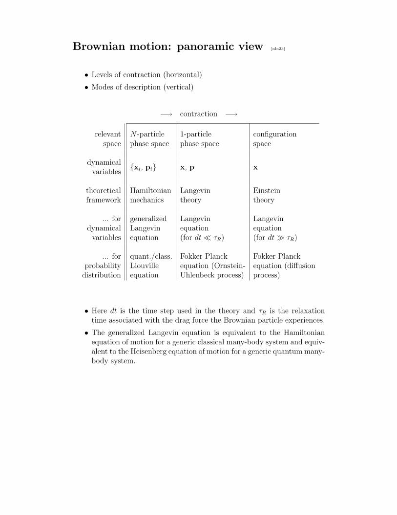
Brownian motion: panoramic view [nln23]

• Levels of contraction (horizontal)

• Modes of description (vertical)

−→ contraction −→

relevant N -particle 1-particle configurationspace phase space phase space space

dynamical xi, pi x, p xvariables

theoretical Hamiltonian Langevin Einsteinframework mechanics theory theory

... for generalized Langevin Langevindynamical Langevin equation equation

variables equation (for dt τR) (for dt τR)

... for quant./class. Fokker-Planck Fokker-Planckprobability Liouville equation (Ornstein- equation (diffusion

distribution equation Uhlenbeck process) process)

• Here dt is the time step used in the theory and τR is the relaxationtime associated with the drag force the Brownian particle experiences.

• The generalized Langevin equation is equivalent to the Hamiltonianequation of motion for a generic classical many-body system and equiv-alent to the Heisenberg equation of motion for a generic quantum many-body system.