0(n - defense technical information center · 0(n simulation techn ique for ... air force packaging...

•4.XPPROVED FOR PUBLIC RELEASE

wDISTRInU§TIOi; U! LI>1ITED AFPEA TECl.'IIC.',L REPORT 'O. 8,-,-u:

In0(n

SIMULATION TECHN IQUE

FOR

EVALUATING CONTAINERS (SIMTEC)Version 2.2

USER'S GUIDE

26 April 1988

(Supersedes Issue of 1 February 1983)

Larry A. Wood

Mechanical Engineer

AUTOVO 787-3120

Commercial (513) 257-3120

MATERIALS ENGINEERING DIVISION ,.

AIR FORCE PACKAGING EVALUATION ACTIVITYAIR FORCE LOGISTICS COMMAND

HQ AFLC/DSTZT

WRIGHT-PATTERSON AFB, OHIO 45433-5999

Special credit should be given to Mr Al Bodnar who developed this model

while performing his functions as an operations research analyst in the

Directorate of Concepts Analysis, Air Force Acquisition Logistics Division,

Wright-Patterson Air Force Base.

... .. ......

fr/i

i 4-0.1

EXECUTIVE SUMMARY

Problem. Few transportation models existed which permitted a program

office to evaluate different types of packaging in terms of life cycle costand sensitivities.

Procedure. The Simulation Technique for Evaluating Containers (SIMTEC), a

computer simulation model, was developed to compare different types ofpackaging and shipping modes and to display the resultant life cycle cost

(LCC). SIMTEC data such as engineering parameters for the containers,shipping rates, basing information, and scenario data are input into the

model. Based on this data, failures, shipping schedules, spare require-

ments, and life cycle costs are generated as outputs. Additionally,

sensitivity runs are available to enable the decision maker to "make the

best decision."

Conclusion. FIMTEC is a model for evaluating different types of packaging

and providing the decision maker with the most realistic data/costavailable at the time. Additionally, SIMTEC can be used to aid theengineer in container design and to estimate the spare requirement needed

to satisfy a particular network. Through simulating the "real world,"

SIMTEC predicts failures, generates a shipping schedule, and evaluates

engineering tradeoffs to lower transportation costs. As with all simula-

tion models, SIMTEC does not give the decision maker a decision, but ratherprovides increased information so a more intelligent decision may result.

ii

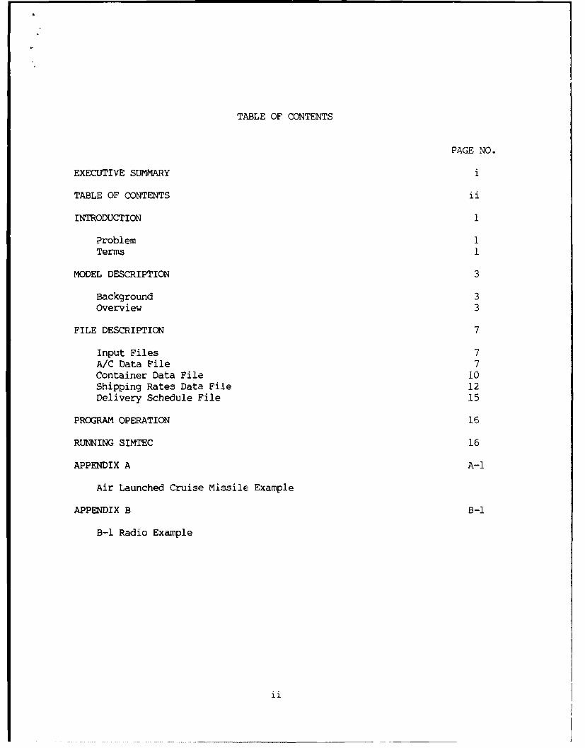
TABLE OF CONTENTS

PAGE NO.

EXECUTIVE SUMMARY i

TABLE OF CONTENTS ii

INTRODUCTION 1

Problem 1Terms 1

MODEL DESCRIPTION 3

Background 3Overview 3

FILE DESCRIPTION 7

Input Files 7A/C Data File 7Container Data File 10Shipping Rates Data File 12Delivery Schedule File 15

PROGRAM OPERATION 16

RUNNING SIMTEC 16

APPENDIX A A-1

Air Launched Cruise Missile Example

APPENDIX B B-1

B-1 Radio Example

ii

INTRODUCTION

Problem. In the past, very few transportation models existed whichpermitted a program to evaluate different types of packaging in terms oflife cycle cost. Models that did exist had few sensitivities availableor did not model the real packaging world via simulation.

Simulation Technique for Evaluating Containers (SIMTEC) is a computerprogram (model) developed to compare different types of packaging in termsof life cycle cost (LCC). Since discussions of computers/modeling can bevery technical-and intimi ating to those unfamiliar with their use, theterms will first be de ed before the technical aspects are discussed in

q7 the next-section.

Terms. A model is a simplified representation of some real worldsituation. Models are used in the place of the real world situation formany reasons-economy and range of experimentation being the more importantones. A model provides the user the means and time to explore the environ-ment solution alternatives, and objectives of the problem in greaterdetail. "I-Eorexample, this model allows the user to evaluate the LCC ofcompetitive con iecadidates and shipping modes (aircraft, truck, etc,)by considering unit cost,-llfe-r weght, distance of shipment, mode of ship-ment, basing information, scenario daete.The computer program is usedto make the modeling procedure more efficient and cost effective.,

In general, a model may be used for the following five purposes:

(1) To study a system for improvement or comparison to anothersystem,

(2) To design a system for the best outcome,

(3) To clarify objectives, goals, or plans7

(4) To train personnel, (:

(5) To predict the results of changes to a system.

SIMTEC, as a specialized model, may be used as a tool to do all of thesethings.

" A simulation model is a model which gives the simplified picture of the"real system." This system can be defined as a set of components (machine,resources, people, etc.-having attributes (output rates, capacities,costs, skills, etc.) which interact. Simulation is the process ofobserving the model in action for the purpose of designing or modifying thesystem.- For example, solar energy thermal collection systems for homes

i t 1

have been tested by simulation, prior to being built, in order to helpsolve particular application problems or to indicate problems in design notknown to exist. Other applications include: production, inventory, anddistribution systems; queuing and traffic flow systems; operating andinformation systems for airports, hospitals, and industrial organizations;environments involving conflict, such as military strategies and competi-tive market Ptrategies.

Simulation provides a means of studying a system, but does not directone to an optimum solution. Such a solution may be found only after aseries of attempts at juggling the variables.

A model, including SIMTEC, never makes a decision. A model provide6information to be used in making a decision. Since a model is of necessitya simplified version of the "real world," it never includes all factorsreally necessary to make a decision.

Of course, the more confidence one has in a model, the more importantits information is ii making a decision. High confidence is obtained in amodel by using real world values as inputs. Lesser confidence is obtainedas you move through estimates towards guesses for your input values. Oftenreal world values are not available and reasonable estimates are the nextbest thing. Anyone with even minimal exposure to data processing has heardof the expression, "garbage in, garbage out." Nowhere is this truer thanin simulation modeling. The best estimates are probably obtained throughinterpretation of historical data or analogies to similar systems. Othersources are formulas, such as those in MIL-STD-794, for determining sizesand weights. The programs for use with Packaging Service Contracts areanother source of cost estimates.

The balance of this user handbook provides the technical details ofusing the SIMTEC computer model. We hope this brief non-technical dis-cussion will clarify the terms/ideas discussed in the technical portionof the user's handbook.

MODEL D3SCRIPTION

Background

Simulation Technique for Evaluating Containers (SIMTEC) is a computerprogram developed to display the lowest life cycle cost and to evaluatecompetitive container candidates and shipping modes (aircraft, truck, etc.)which satisfy all mission requirements. While Packaging, Handling, andTransportation (PH&T) is often ignored since the dollars involved arerelatively small when compared to major program acquisitions, PHiT is anarea where real savings do exist.

This model was originally developed for the Air Launched Cruise Missile(ALCM) engine program to evaluate alternative containers to ship the ALCMengine. (Reference Appendix A for an example use of tne model and theresults of the original ALCM program). SIMTEC is a generalized extensionof this original study. The major addition to the original model is themethod of generating zhipments. The ALCM program was based solely uponscheduled maintenance since a missile does not fail due to flying hourslike aircraft. SIMTEC predicts failures and generates a shipping schedulebased upon engineering and logistics data. (The method of estimatingfailures is discussed later in this guide). SIMTEC is not only for newacquisition programs but can be used for evaluating replacement containersfor existing systems.

Oerview

SIMTEC uses data from several sources to make its evaluation. The datacan either be actual engineering and logistics inputs or estimates. Ifonly estimates are available, SIMTEC can do sensitivity runs to give thedecision-maker a better feel for the environment so a better decision mayresult.

The first of four sets of data includes program control information,engineering data, basing information, scenario data, plus other informationas discussed in this manual. Based upon this data file SIMTEC will predictfailures and a subsequent shipping schedule. A random seed number is usedto begin these calculations. This random seed number generates differentrandom numbers from a uniform distribution. (Using different seed numberswill generate ditferent sequences of random numbers, and therefore,different failure predictions). Unless the analyst desires to evaluate theeffects of another profile of failures, the shipping schedule needs only tobe predicted once. This results in a shortened run time for SIMTEC.

The second set of data are the engineering parameters for the containercandidates. Four elements were chosen that were deemed appropriate toevaluate container differences: cost, life, weight, and packing/unpackinglabor expense. Container size was excluded since this element would be

3

similar among the candidates while cost, life, weight, and packaging timewould all relate to the particular materials and design of eachalternative. Note: If a new container is going to be designed to satisfya particular shipping network, SIMTEC can also be used to find the best mixof these four elements.

The third set of data are the shipping rates to estimate the life cycleshipping expense. These rates are based upon cost per hundred pounds andcan vary due to the size of shipment, the distance of shipment, and themode of transportation.

TShe fourth, or final, set of data includes the production and sparesdelivery schedules. This is an unformatted or "Random Access" file andtherefore cannot be tvoed out. Simtec will display this data and provideopportunity for revision.

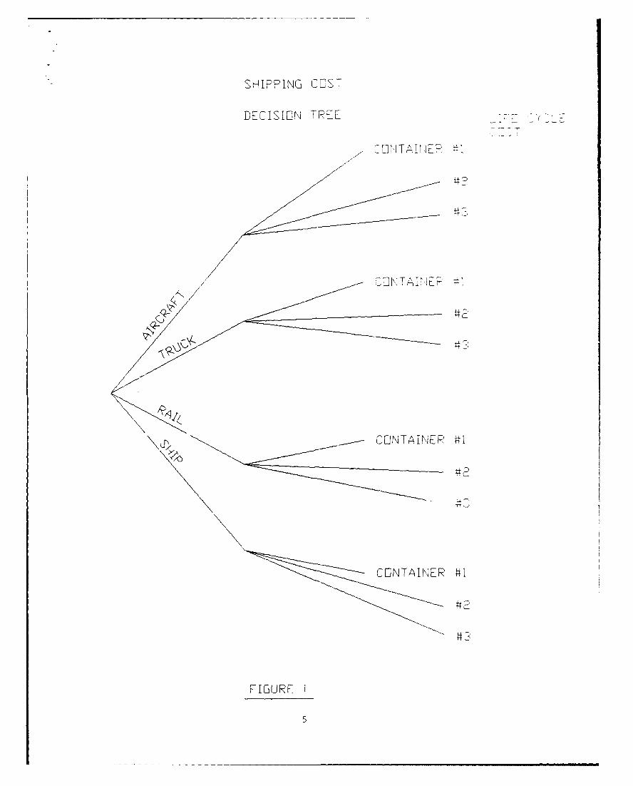
Figure 1 is a tree diagram illustrating the trade-offs available tolower transportation costs. Collecting shipping rates for all feasiblemodes of transportation and collecting data for all feasible containersprovides the data to evaluate all options and select an option based uponlowest life cycle cost. The purpose of this model is to provide a meansof evaluating life cycle cost differences among feasible PH&T options.

-_:HIPPING CEST

LESI'SIN TREE

\'p, CENTAINEP #1

-CONTAINER #1

FIGURF

5

As a last note, SIMTEC has uses other than as a container evaluationtechnique. SIMTEC can help a container engineer design a container or canestimate the spares requirements (by inputing zero spares into theschedule) that will be necessary to satisfy a particular network. Thisspares value could change based upon the mode of transportation (forexample, truck versus airlift) if shortened pipeline time results. Thenumber of shipments per month could also affect the spares requirement.

As with all simulation models, SIMTEC does not give the decisionmaker a decision, but only increases information so a better decisioncan be made. There may be other factors that will also influence adecision. For example, this model assumes each container alternativeprovides adequate protection from damage (i.e., SIMTEC assumes allcontainers are equal). If the equipment is extremely expensive andfragile, an increase in shipping expense by not choosing the lowestlife cycle cost container may be warrantpd. (Lowest life cycle costis desirable, but item protection is a necessity). These types ofcontingencies can be evaluated outside of SIMTEC. The cost differencebetween competing containers will aid in making this type of decision.

FILE DESCRIPTION

Input Files

Four input data files (A/C Data, Container Data, Shipping Rates,

Delivery Schedule) are needed to provide the necessary information to run

SIMTEC. This input can be provided either by the use of previously

existing files or by an interactive routine at the beginning of the

program. This input routine asks for the necessary data and creates fileson disk to run the program later without re-entering the data.

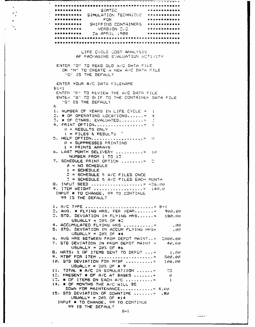
A/C Data File

The "A/C Data" file provides program control information plus

engineering and operational data to generate failures and the subsequent

shipping schedule. Figures 1 and 3 illustrate an example A/C data file.

This example shows data for an item, i.e., a radio used on the BI

program. Note that data is needed for both the aircraft and the item being

evaluated. Aircraft data describes the environment within which the itemwill be operated. The required data describes how often each item on

each aircraft will actually be operating. Item level data also describes

how reliable, how many items on each aircraft, and how often shipments

must be made (maintenance concept) for each item failure. Note that

these parameters may differ for the same item on different aircraft due

to operating locations and applications. Figure 2 shows the aircraft

data, number of flying hours, item failure rate, and related information

required.

Figure 3 shows the detailed information for this aircraft at each

operating location. All the information contained in these two Figures is

stored in the "A/C Data" file. (Reference file Bl-l).

7I

R1. NUMBER OF YEARS IN LIFE CYCLE = 1

2. NUMBER OF OPERATING LOCATIONS = 4

3. NUMBER OF CTNRS, EVALUATED... = 34. PRINT OPTION ................. = 1

0 = RESULTS ONLYI = FILES & RESULTS

5. HELP OPTION .................. = 0

O SUPPRESSES PRINTING1 = PRINTS ARRAYS

6 LAST MONTh DELIVERY .......... = 10

NUMBER FROM 1 TO 137. SCHEDULE PRINT OPTION ........ = 2

0 = NO SCHEDULE1 = SCHEDULE2 = SCHEDULE & A/C FILES ONCE

3 = SCHEDULE & A/C FILES EACH MONTH8. INPUT SEED ................... = -26.009. ITEM WEIGHT .................. = 140.099

1. A/C TYPE ............................ B-i

2. AVG. # FLYING HRS. PER YEAR ........ = 900.00

3. STD. DEVIATION INN FLYING HRS ..... = 180.00

USUALLY = 20% OF #24. ACCUMULATED FLYING HRS ............. = .00

5. STD. DEVIATION IN ACCUM FLYING HRS = .00

USUALLY = 20% OF #46. AVG HRS BETWEEN PRGM DEPOT MAINT.. = 2000.007. STD DEVIATION IN PRGM DEPOT MAIN.. = 40.00

USUALLY = 20% OF #6

8. NRTS: % OF ITEMS SENT TO DEPOT .... = 1.009. MTBF FOR ITEM ..................... = 500.0010. STD DEVIATION FOR MTBF ........... = 100.00

USUALLY = 20% OF #911. TOTAL # A/C IN SIMULATION ........ = 3512. PRESENT # OF A/C AT BASES ........ = 0

13. NUMBER OF ITEMS ON EACH A/C ...... = 114. NUMBER OF MONTHS THE A/C WILL BE

DOWN FOR MAINTENANCE .......... = 4.0015. STD DEVIATION OF DOWNTIME ......... = .80

USUALLY = 20% OF #14INPUT # TO CHANGE, 99 TO CONTINUE

99

FIGURE 2

13

THE NUMBER OF OPERATING LOCATIONS = 4INFO FOR LOCATION 1

1. NUMBER OF A/C .................. = 162. MONTH THE A/C ARRIVE ........... = 2

ENTER THE # TO CHANGE, 99 TO CONTINUE99


1. NUMBER OF A/C- ................ = 52. MONTH THE A/C ARRIVE .......... 5



1. NUMBER OF A/C ................ = 102. MONTH THE A/C ARRIVE ......... = 7



1. NUMBER OF A/C .................= 42. MONTH THE A/C ARRIVE ......... = 8


FIGURE 3

9

NOTE: This 13 months/year is typically used in the business world. It isdetermined by dividing 52 weeks by 4 weeks for a month. This alleviatesany problems of how to handle the extra days in the months). B-1(2,5,7,8).

In this example all aircraft are new. If the aircraft are already inthe inventory, then the "Month the A/C Arrive" data element would not beneeded (no value would be entered) and the record would be entered beforean new deliveries. The delivery schedule needs to be input in order. Theorder of bases is not important, i.e., deliveries to base 4 can be beforebase 3 because the timing of the deliveries control the program not thebasing itself.

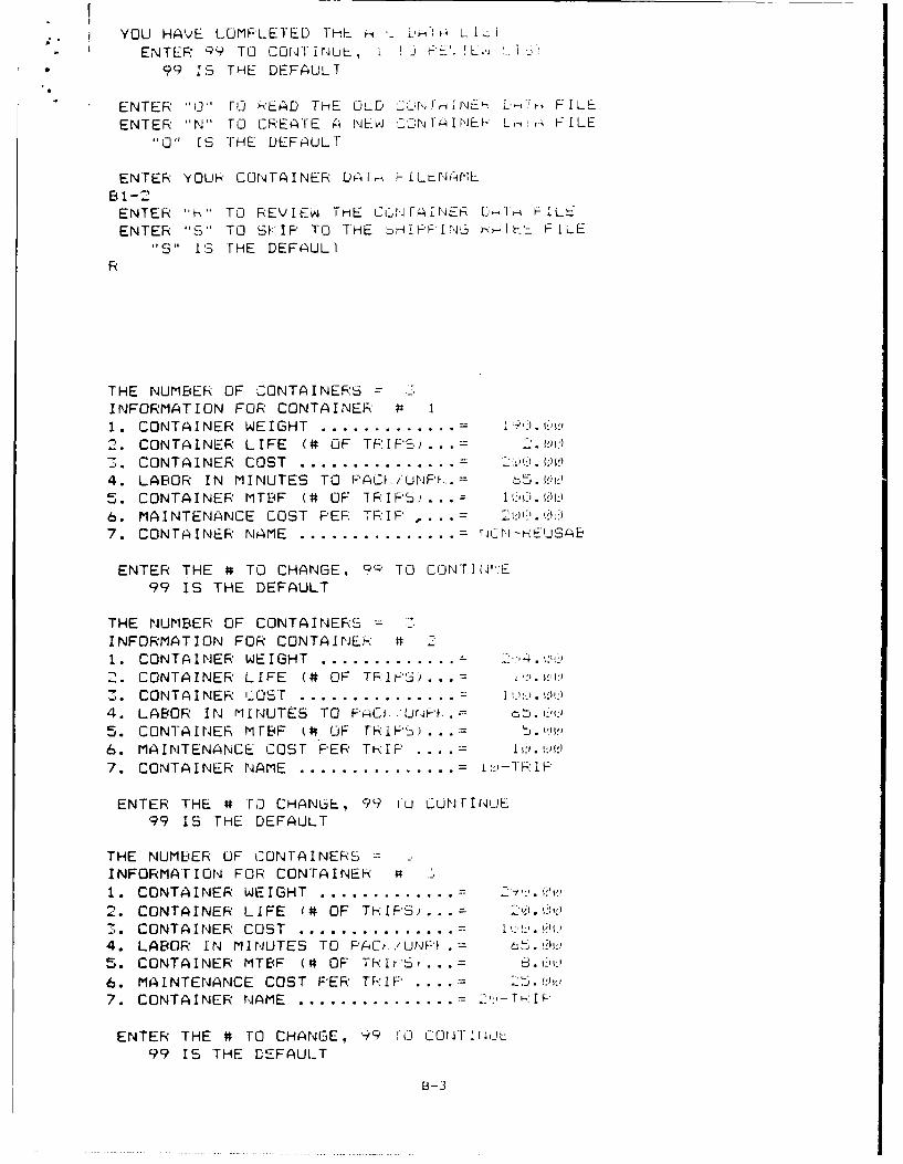
Container Data File

The "Container Data" file contains all pertinent container data and isthe basis for the evaluation. Information includes container weight, life,cost, and pack/unpack time. Figure 4 is an example "Container Data" file.

The information contained in figure 4 is stored in file Bl-2.

10

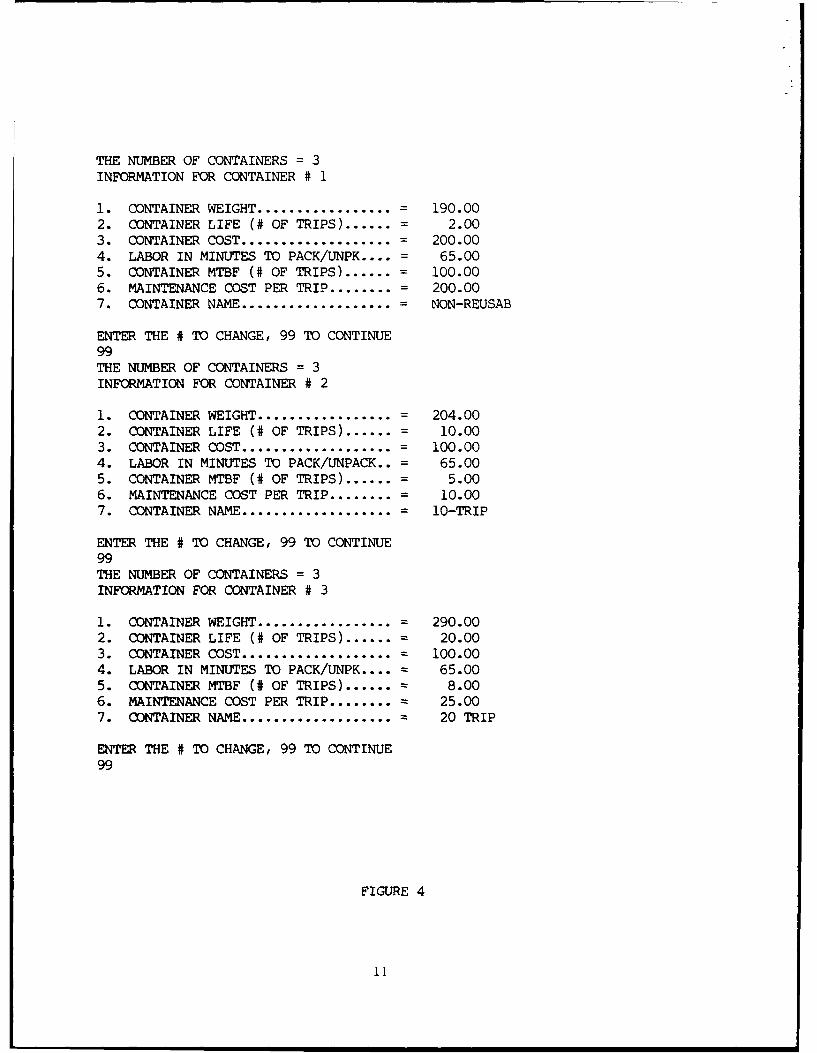
THE NUMBER OF CONTAINERS = 3INFORMATION FOR CONTAINER # 1

1. CONTAINER WEIGHT ................. = 190.002. CONTAINER LIFE (# OF TRIPS) ...... = 2.003. CONTAINER COST ................... = 200.004. LABOR IN MINUTES TO PACK/UNPK .... = 65.005. CONTAINER MTBF (# OF TRIPS) ...... = 100.006. MAINTENANCE COST PER TRIP ........ = 200.007. CONTAINER NAME ................... = NON-REUSAB

ENTER THE # TO CHANGE, 99 TO CONTINUE99THE NUMBER OF CONTAINERS = 3INFORMATION FOR CONTAINER # 2

1. CONTAINER WEIGHT ................. = 204.002. CONTAINER LIFE (# OF TRIPS) ...... = 10.003. CONTAINER COST ................... = 100.004. LABOR IN MINUTES TO PACK/UNPACK.. = 65.005. CONTAINER MTBF (# OF TRIPS) ...... = 5.006. MAINTENANCE COST PER TRIP ........ = 10.007. CONTAINER NAME ................... = 10-TRIP

ENTER THE # TO CHANGE, 99 TO CONTINUE99THE NUMBER OF CONTAINERS = 3INFORMATION FOR CONTAINER # 3

1. CONTAINER WEIGHT ................. = 290.002. CONTAINER LIFE (# OF TRIPS) ...... = 20.003. CONTAINER COST ................... 100.004. LABOR IN MINUTES TO PACK/UNPK .... = 65.005. CONTAINER MTBF (# OF TRIPS) ....... = 8.006. MAINTENANCE COST PER TRIP ......... = 25.007. CONTAINER NAME ................... = 20 TRIP


FIGURE 4

i1

NOTE: MTBF (5) and MAINTENANCE (6) data elements can be used in two ways:

a. As the number of trips between maintenance with its associatedmaintenance costs.

b. As the probability that a container is destroyed. If this is thecase, the maintenance cost would equal the acquisition cost of a container/its contents. The following table illustrates values to be used (assumingprobabilities of failures on one-way trips). For probabilities of failureon a round trip, double the MMTBF.

Prob 1% 10% 20% 50%

MMTBF 100 10 5 2

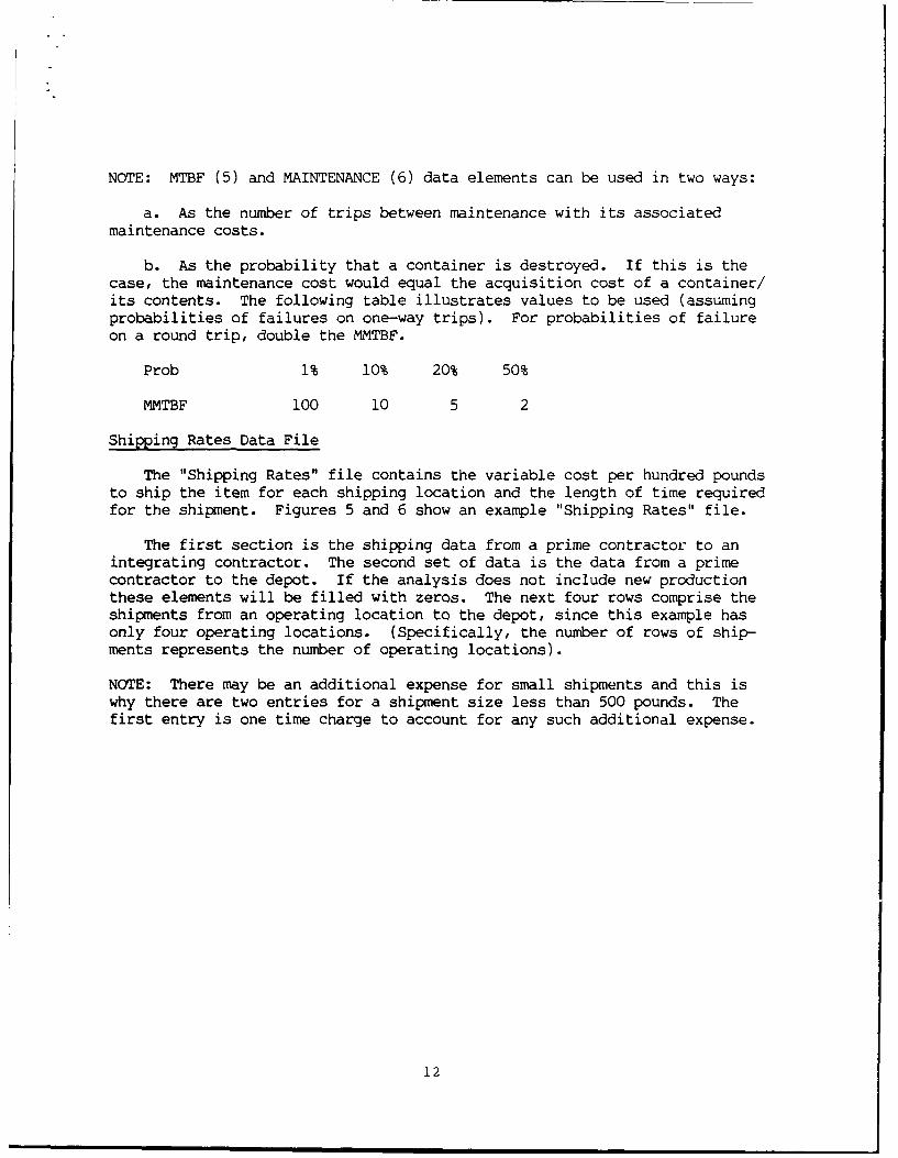
Shipping Rates Data File

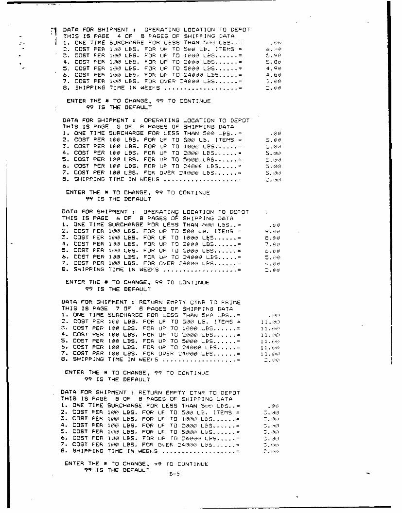
The "Shipping Rates" file contains the variable cost per hundred poundsto ship the item for each shipping location and the length of time requiredfor the shipment. Figures 5 and 6 show an example "Shipping Rates" file.

The first section is the shipping data from a prime contractor to anintegrating contractor. The second set of data is the data from a primecontractor to the depot. If the analysis does not include new productionthese elements will be filled with zeros. The next four rows comprise theshipments from an operating location to the depot, since this example hasonly four operating locations. (Specifically, the number of rows of ship-ments represents the number of operating locations).

NOTE: There may be an additional expense for small shipments and this iswhy there are two entries for a shipment size less than 500 pounds. Thefirst entry is one time charge to account for any such additional expense.

12

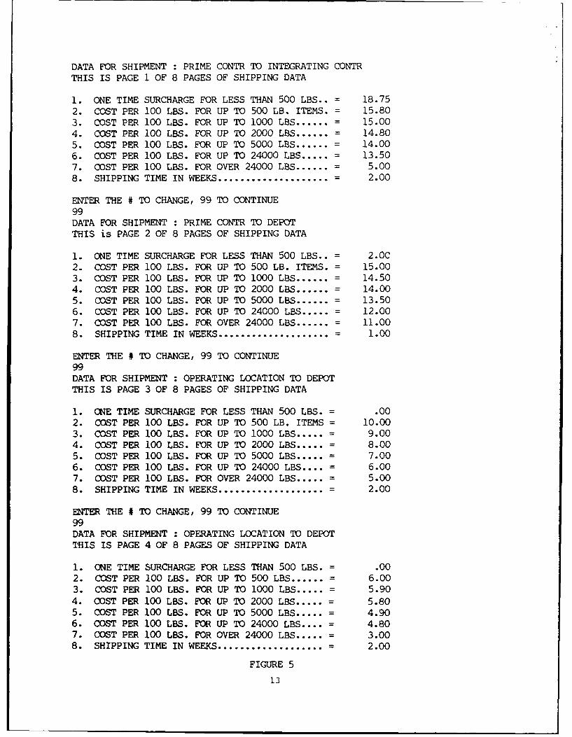
DATA FOR SHIPMENT : PRIME CONTR TO INTEGRATING CONTRTHIS IS PAGE 1 OF 8 PAGES OF SHIPPING DATA

1. ONE TIME SURCHARGE FOR LESS THAN 500 LBS.. = 18.752. COST PER 100 LBS. FOR UP TO 500 LB. ITEMS. = 15.803. COST PER 100 LBS. FOR UP TO 1000 LBS ...... = 15.004. COST PER 100 LBS. FOR UP TO 2000 LBS ...... = 14.80

5. COST PER 100 LBS. FOR UP TO 5000 LBS ...... = 14.006. COST PER 100 LBS. FOR UP TO 24000 LBS ..... = 13.50

7. COST PER 100 LBS. FOR OVER 24000 LBS ...... = 5.00

8. SHIPPING TIME IN WEEKS .................... = 2.00

ENTER THE # TO CHANGE, 99 TO CONTINUE99DATA FOR SHIPMENT : PRIME CONTR TO DEPOTTHIS is PAGE 2 OF 8 PAGES OF SHIPPING DATA

1. ONE TIME SURCHARGE FOR LESS THAN 500 LBS.. = 2.OC2. COST PER 100 LBS. FOR UP TO 500 LB. ITEMS. = 15.003. COST PER 100 LBS. FOR UP TO 1000 LBS ...... = 14.504. COST PER 100 LBS. FOR UP TO 2000 LBS ...... = 14.00

5. COST PER 100 LBS. FOR UP TO 5000 LBS ...... = 13.50

6. COST PER 100 LBS. FOR UP TO 24000 LBS ..... = 12.00

7. COST PER 100 LBS. FOR OVER 24000 LBS ...... = 11.00

8. SHIPPING TIME IN WEEKS .................... = 1.00

ENTER THE # TO CHANGE, 99 TO CONTINUE99DATA FOR SHIPMENT : OPERATING LOCATION TO DEPOTTHIS IS PAGE 3 OF 8 PAGES OF SHIPPING DATA

1. ONE TIME SURCHARGE FOR LESS THAN 500 LBS. = .002. COST PER 100 LBS. FOR UP TO 500 LB. ITEMS = 10.003. COST PER 100 LBS. FOR UP TO 1000 LBS ..... = 9.004. COST PER 100 LBS. FOR UP TO 2000 LBS..... = 8.005. COST PER 100 LBS. FOR UP TO 5000 LBS ..... = 7.006. COST PER 100 LBS. FOR UP TO 24000 LBS .... = 6.007. COST PER 100 LBS. FOR OVER 24000 LBS ..... = 5.008. SHIPPING TIME IN WEEKS ................... = 2.00


1. ONE TIME SURCHARGE FOR LESS THAN 500 LBS. = .002. COST PER 100 LBS. FOR UP TO 500 LBS ...... = 6.003. COST PER 100 LBS. FOR UP TO 1000 LBS ..... = 5.904. COST PER 100 LBS. FOR UP TO 2000 LBS ...... = 5.80

5. COST PER 100 LBS. FOR UP TO 5000 LBS ..... = 4.90

6. COST PER 100 LBS. FOR UP TO 24000 LBS .... = 4.807. COST PER 100 LBS. FOR OVER 24000 LBS ..... = 3.00

8. SHIPPING TIME IN WEEKS ................... = 2.00

FIGURE 5

13


1. ONE TIME SURCHARGE FOR LESS THAN 500 LBS.. = .002. COST PER 100 LBS. FOR UP TO 500 LB. ITEMS. = 5.003. COST PER 100 LBS. FOR UP TO 1000 LBS ...... = 5.004. COST PER 100 LBS. FOR UP TO 2000 LBS ...... = 5.005. COST PER 100 LBS. FOR UP TO 5000 LBS ...... = 5.006. COST PER 100 LBS. FOR UP TO 24000 LBS ..... = 5.007. COST PER 100 LBS. FOR OVER 24000 LBS ...... = 5.008. SHIPPING TIME IN WEEKS .................... = 2.00


1. ONE TIME SURCHARGE FOR LESS THAN 500 LBS.. = .002. COST PER 100 LBS. FOR UP TO 500 LB. ITEMS. = 9.003. COST PER 100 LBS. FOR UP TO 1000 LBS ...... = 8.004. COST PER 100 LBS. FOR UP TO 2000 LBS ...... = 7.005. COST PER 100 LBS. FOR UP TO 5000 LBS ...... = 6.006. COST PER 100 LBS. FOR UP TO 24000 LBS ..... = 5.007. COST PER 100 LBS. FOR OVER 24000 LBS ...... = 4.008. SHIPPING TIME iN WEEKS .................... = 2.00

ENTER THE # TO CHANGE, 99 TO CONTINUE99DATA FOR SHIPMENT : RETURN EMPTY CTNR TO PRIMETHIS IS PAGE 7 OF 8 PAGES OF SHIPPING DATA

1. ONE TIME SURCHARGE FOR LESS THAN 500 LBS. = .002. COST PER 100 LBS. FOR UP TO 500 LB. ITEMS = 11.003. COST PER 100 LBS. FOR UP TO 1000 LBS ..... = 11.004. COST PER 100 LBS. FOR UP TO 2000 LBS ..... = 11.005. COST PER 100 LBS. FOR UP TO 5000 LBS ..... = 11.006. COST PER 100 LBS. FOR UP TO 24000 LBS .... = 11.007. COST PER 100 LBS. FOR OVER 24000 LBS ..... = 11.008. SHIPPING TIME IN WEEKS ................... = 2.00

ENTER THE # TO CHANGE, 99 TO CONTINUE99DATA FOR SHIPMENT : RETURN EMPTY CTNR TO PRIMETHIS IS PAGE 8 OF 8 PAGES OF SHIPPING DATA

1. ONE TIME SURCHARGE FOR LESS THAN 500 LBS. = .002. COST PER 100 LBS. FOR UP TO 500 LBS ...... = 3.003. COST PER 100 LBS. FOR UP TO 1000 LBS ..... = 3.004. COST PER 100 LBS. FOR UP TO 2000 LBS ..... = 3.005. COST PER 100 LBS. FOR OP TO 5000 LBS ..... = 3.006. COST PER 100 LBS. FOR UP TO 24000 LBS .... = 3.007. COST PER 100 LBS. FOR OVER 24000 LBS ..... = 3.008. SHIPPING TIME IN WEEKS ................... = 2.00

FIGURE 6

14

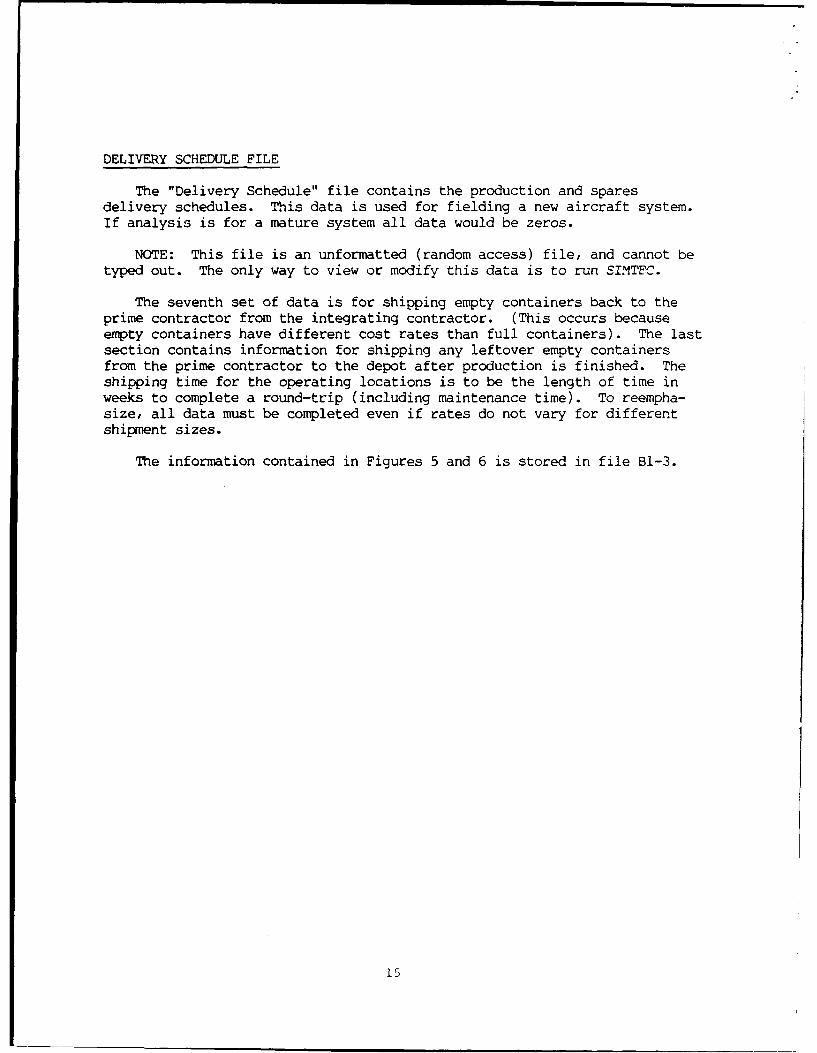
DELIVERY SCHEDULE FILE

The "Delivery Schedule" file contains the production and sparesdelivery schedules. This data is used for fielding a new aircraft system.If analysis is for a mature system all data would be zeros.

NOTE: This file is an unformatted (random access) file, and cannot betyped out. The only way to view or modify this data is to run SIMTFC.

The seventh set of data is for shipping empty containers back to theprime contractor from the integrating contractor. (This occurs becauseempty containers have different cost rates than full containers). The lastsection contains information for shipping any leftover empty containersfrom the prime contractor to the depot after production is finished. Theshipping time for the operating locations is to be the length of time inweeks to complete a round-trip (including maintenance time). To reempha-size, all data must be completed even if rates do not vary for differentshipment sizes.

The information contained in Figures 5 and 6 is stored in file B1-3.

15

PROGRAM OPERATION

Throughout the remainder of this guide, all underlined words are to be

typed in by the user. A carriage return is indicated by the symbol "i".

SIMTEC is programmed for use on IBM-PC compatible computers. OperatingSIMTEC on other computer systems will necessitate code changes so the modelcan interface with the system. Most changes will center around system-unique requirements since SIMTEC is written in FORTRAN 77.

Because SIMTEC requires extensive file manipulation it should be loadedonto a Winchester-type hard disk before running. Operation from the floppy

disk will be very time consuming.

Copy the entire floppy disk using the copy *.* MSDOS Command, then put

the floppy disk in a safe place as a backup disk.

If you elect to run SIMTEC from the floppy disk you should first make a

backup copy using the procedure outlined above.

RUNNING SIMTEC

"7" You are now ready to run SIMTEC. Input the following command atthe prompt:

7SIMTEC

A series of questions follow this command allowing the user to attach,create, and/or modify data files. Sample files are provided for instruc-tion, refer to Appendix B for file names. The user can enter values or useexisting data for production delivery schedules, spares delivery schedules,and predict a new monthly failure distribution. If there is a change toeither or both delivery schedules, the program will enable the user toinput the month and the number of containers that are to arrive. If thereare no changes to be made, the program will omit the additional questionsand the shipping rates file, and the results, provided number 4 PrintOption = 1. If the print option = 0, then only the results will beprinted, the "Operating Location Record", and "Aircraft Record" sche% uleswill be suppressed.

An example printout of the program operation is included in AppendixB.

Note that the printout consists of an input routine for file management, ashipping schedule, container data, shipping cost, and container programs(one for each option). These areas are discussed in detail below.

16

Shipping Schedules

The shipping schedule is a permanent file created by SIMTEC. If a newproduction or spare delivery is required, all monthly deliveries must bechanged since all previous data will be retained until updated. Once the

complete schedule is created, the run time of SIMTEC is shortened (if no

changes are required and failures need not be predicted), and SIMTEC willuse the previously predicted data to evaluate additional containers or todo sensitivity runs. Note that the first two lines of the shippingschedule are input while the remaining four lines are computer generated.

1. # of FAILURES = Total of the computer generated output in theshipping schedule. (Last 4 lines in this particular case.) This is acomputer generated value.

2. # of SHIPMENTS = # of failures times the NRTS rate. (In this casethe NRTS rate is 1.0, so the number of shipments = number of failures).This is a computer generated value.

3. MONTH = How long it ran. (In this case the model ran for 13 months- 1 business year.) This value is a computer generated value.

Container Data. The data is input on the "Container Data" data file.

Shipping Data. The values in this table are input on the "Shipping Rates"data file.

Container Program. These values are all computer generated. Note thatthere are 3 of these - one for each type of shipping container evaluated.

1. TOTAL CONTAINERS total number of containers needed to satisfy

shipping schedule using a particular container.

2. SPARE STORAGE = number of containers used to store an item.

3. PROD SHIP = number of containers used as production containers.

4. CONTAINER COST = total cost of container being evaluated.

5. SHIPPING COST = total cost of shipping the containers.

6. PACK/UNPACK COST = total cost to pack and unpack the containers.

17

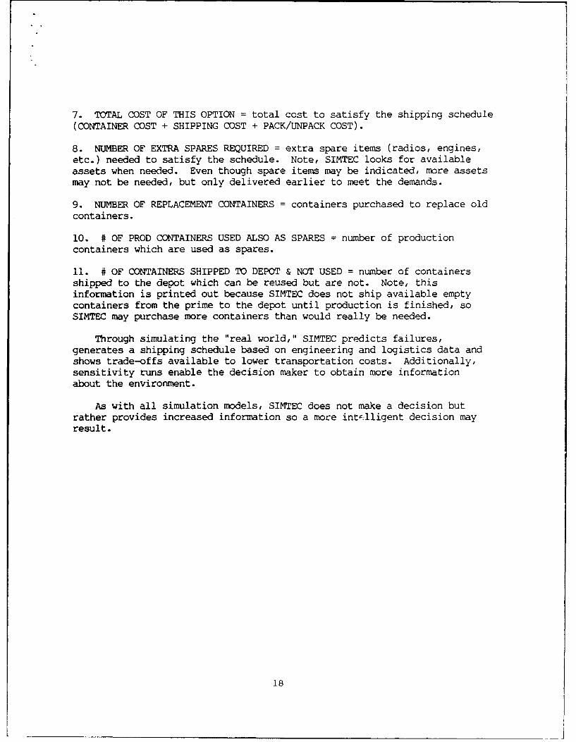
7. TOTAL COST OF THIS OPTION = total cost to satisfy the shipping schedule(CONTAINER COST + SHIPPING COST + PACK/UNPACK COST).

8. NUMBER OF EXTRA SPARES REQUIRED = extra spare items (radios, engines,etc.) needed to satisfy the schedule. Note, SIMTEC looks for availableassets when needed. Even though spare items may be indicated, more assetsmay not be needed, but only delivered earlier to meet the demands.

9. NUMBER OF REPLACEMENT CONTAINERS = containers purchased to replace oldcontainers.

10. # OF PROD CONTAINERS USED ALSO AS SPARES = number of productioncontainers which are used as spares.

11. # OF CONTAINERS SHIPPED TO DEPOT & NOT USED = number of containersshipped to the depot which can be reused but are not. Note, thisinformation is printed out because SIMTEC does not ship available emptycontainers from the prime to the depot until production is finished, soSIMTEC may purchase more containers than would really be needed.

Through simulating the "real world," SIMTEC predicts failures,generates a shipping schedule based on engineering and logistics data andshows trade-offs available to lower transportation costs. Additionally,sensitivity runs enable the decision maker to obtain more informationabout the environment.

As with all simulation models, SIMTEC does not make a decision butrather provides increased information so a more intc'lligent decision mayresult.

18

APPENDIX A

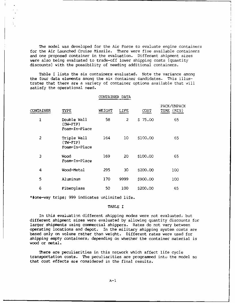
The model was developed for the Air Force to evaluate engine containersfor the Air Launched Cruise Missile. There were five available containersand one proposed container in the evaluation. Different shipment sizeswere also being evaluated to trade-off lower shipping costs (quantitydiscounts) with the possibility of needing additional containers.

Table I lists the six containers evaluated. Note the variance amongthe four data elements among the six container candidates. This illus-trates that there are a variety of container options available that willsatisfy the operational need.

CONTAINER DATA

PACK/UNPACK

CONTAINER TYPE WEIGHT LIFE COST TIME (MIN)

1 Double Wall 58 2 $ 75.00 65(DW-FIP)Foam-In-Place

2 Triple Wall 164 10 $100.00 65(TW-FIP)Foam-In-Place

3 Wood 169 20 $100.00 65Foam-In-Place

4 Wood-Metal 295 30 $200.00 100

5 Aluminum 170 9999 $900.00 100

6 Fiberglass 50 100 $200.00 65

*#one-way trips; 999 indicates unlimited life.

TABLE I

In this evaliation different shipping modes were not evaluated, butdifferent shipment sizes were evaluated by allowing quantity discounts forlarger shipments using commercial shippers. Rates do not vary betweenoperating locations and depot. In the military shipping system costs arebased only on volume rather than weight. Different rates were used forshipping empty containers, depending on whether the container material iswood or metal.

There are peculiarities in this network which affect life cycletransportation costs. The peculiarities are programmed into the model sothat cost effects are considered in the final results.

A-i

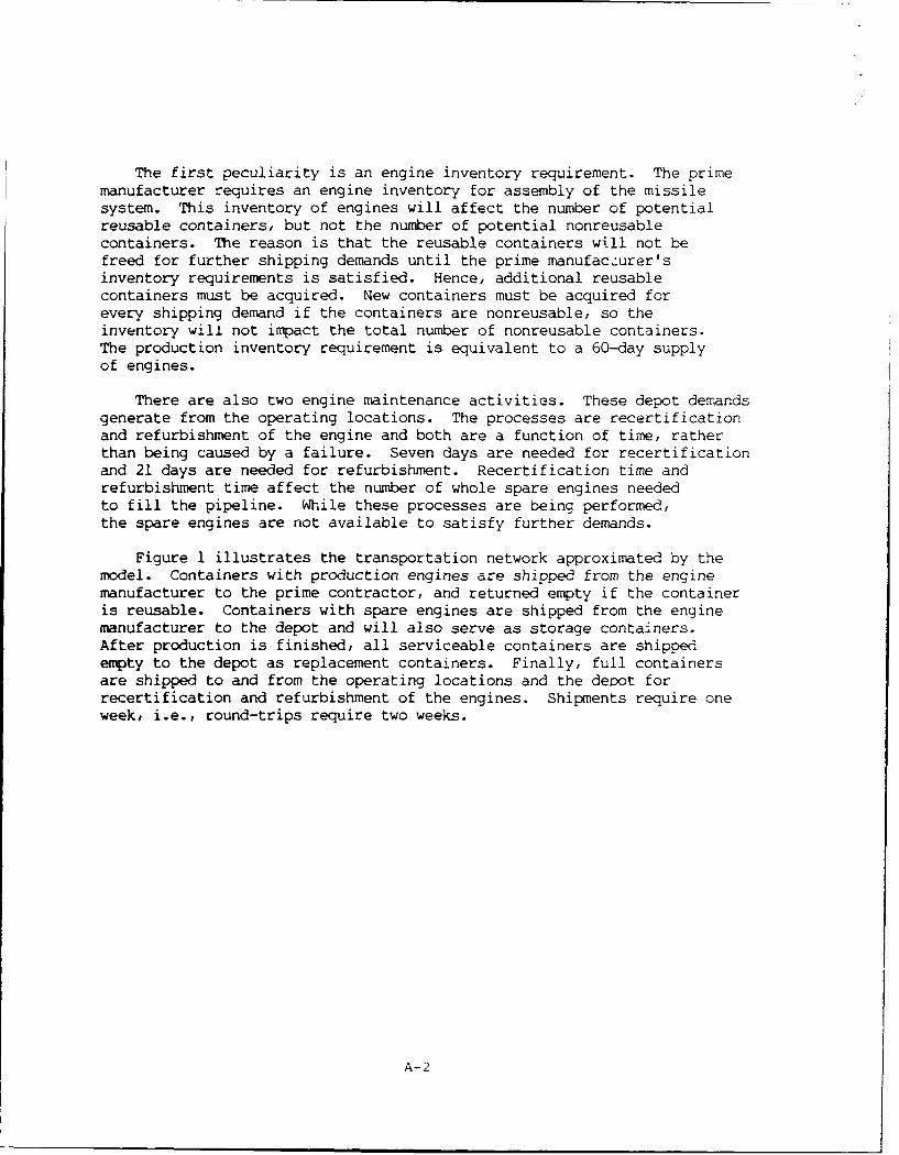
The first peculiarity is an engine inventory requirement. The primemanufacturer requires an engine inventory for assembly of the missilesystem. This inventory of engines will affect the number of potentialreusable containers, but not the number of potential nonreusablecontainers. The reason is that the reusable containers will not befreed for further shipping demands until the prime manufac:urer'sinventory requirements is satisfied. Hence, additional reusablecontainers must be acquired. New containers must be acquired forevery shipping demand if the containers are nonreusable, so theinventory will not impact the total number of nonreusable containers.The production inventory requirement is equivalent to a 60-day supplyof engines.

There are also two engine maintenance activities. These depot demandsgenerate from the operating locations. The processes are recertificationand refurbishment of the engine and both are a function of time, ratherthan being caused by a failure. Seven days are needed for recertificationand 21 days are needed for refurbishment. Recertification time andrefurbishment time affect the number of whole spare engines neededto fill the pipeline. While these processes are being performed,the spare engines are not available to satisfy further demands.

Figure 1 illustrates the transportation network approximated by themodel. Containers with production engines are shipped from the enginemanufacturer to the prime contractor, and returned empty if the containeris reusable. Containers with spare engines are shipped from the enginemanufacturer to the depot and will also serve as storage containers.After production is finished, all serviceable containers are shippedempty to the depot as replacement containers. Finally, full containersare shipped to and from the operating locations and the derpot forrecertification and refurbishment of the engines. Shipments require oneweek, i.e., round-trips require two weeks.

A-2

SHIPPING NET/ORK

PRIME CGNTRACTO

ENGINE CONTRACTER_

DEPOT

FIGIUE 1

RESULTS

The fiberglass container shows the lowest life cycle cost, used forboth production and depot deliveries, among the six containers evaluated.The fiberglass container is the most economical container because its dataelements were most suited for this shipping network with its constraints.Long life, low weight, moderate cost, and moderate labor expense are allassociated with the fiberglass container. For another shipping network,with its own schedule, rates, and constraints another container may be moreeconomical than the fiberglass optioun. Table II shows possible costsavings from using the fiberglass container. The fiberglass containersshows a cost advantage of over $250,000 when compared to W-FIP container,the next lowest cost option, and this does not include the cost of foam-in-place equipment. Also shown is that transportation costs can double byselecting an inappropriate container. The wood-metal option has atransportation expense twice the transportation expense of the fiberglassoption.

A-3

COST COMPARISON

DEV CONT SHIP PK/UNPK TOTALCONT COST COST COST COST COST

TW-FIP 2,162 $ 0 $216,200 $777,630 $108,147 $1,101,977FIBERG 371 6,000 74,200 656,910 108,147 845,257DIFFER 1,791 ($6,000) $142,000 $120,720 $ 0 $ 256,720

WD-MET 784 $ 0 $156,800 $1,249,741 $299,484 $1,706,025FIBERG 371 6,000 $ 74,200 656,910 108,147 845,257DIFFER 413 ($6,000) $ 82,600 $ 592,831 $191,337 $ 860,768

TABLE II

The fiberglass option is the only container which has not been fullydeveloped, so the data for the container are engineering estimates. Asensitivity analysis was performed because of the uncertainty related todata for a container requiring additional development. Also, thesensitivity analysis highlights cost drivers that affect transportationcosts which illustrates another use of the model.

Weight sensitivity is evaluated by steadily increasing the weight ofthe fiberglass container while holding engine weight constant. Figure IIIis a graph showing the weight line. As shown, the fiberglass optionremains as the lowest cost option as long as the weight of the containerincluding engine is less than 250 pounds.

VEIGHT SENSITIVITY

1.2 - / o

TW-FIP

1.1

1930 210 230 250 2 7 0 g:

FIGURE 3

A-4

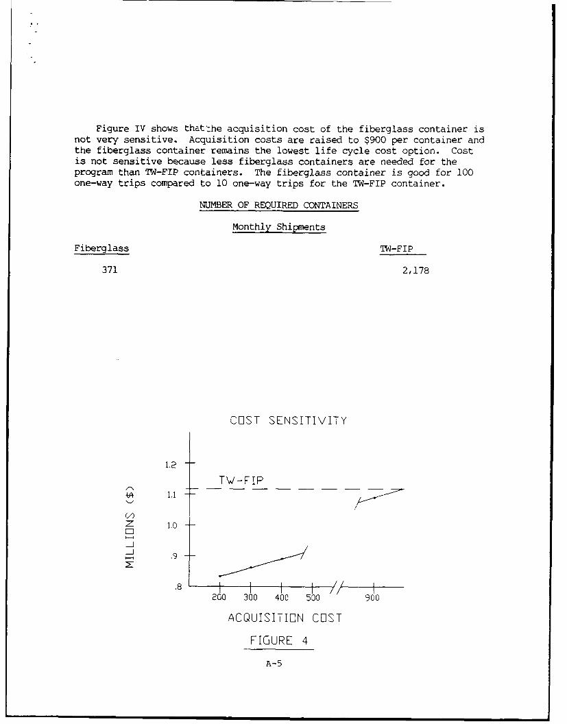
Figure IV shows thatthe acquisition cost of the fiberglass container isnot very sensitive. Acquisition costs are raised to $900 per container andthe fiberglass container remains the lowest life cycle cost option. Costis not sensitive because less fiberglass containers are needed for theprogram than T:U-FIP containers. The fiberglass container is good for 100one-way trips compared to 10 one-way trips for the TW-FIP container.

NUMBER OF REQUIRED CONTAINERS

Monthly Shipments

Fiberglass TW-FIP

371 2,178

CIST SENSITIVITY

1.2

TW-FIP

(A1.0

z/

.8200 300 400 500 900

ACQUISITION COIST

FIGURE 4

A-5

Durability sensitivity shows that as long as the life of the fiberglasscontainer is greater than 75 one-way trips, costs do not change. When thelife drops below 60 trips, costs begin to rise since more and morereplacement containers are needed. Figure V illustrates the durabilitysensitivity.

COINTAINER DURABILITY

1.6-

-' 1.4 -

z 1,3-

1,2 TW-FIPi

1,0.8 I I I I

20 40 60 80 100

NUMBER OF TRIPS

FIGURE 5

Pack/unpack sensitivity is not evaluated since the data used isconsidered a worse possible case, and a much lower pack/unpack time isexpected in reality.

A-6

APPENDIX B

SIMTEC

********** SIMULATION TECHNIUE

FORSHIPPING CONTAINERS

VERSION 2.2

26 APRIL 1983

LIFE C'YCLE COST ANALYSIn

AF PACKAGING EVALUATION ATIVITY

ENTER "0" TO READ OLD A/C DATA FILE

OR "N" TO CREATE A NEW A/C DATA FILE"0" IS THE DEFAULT

ENTER YOUR A/C DATA FILENAME

bi-i

ENTER '"R" TO REVIEW THE A/C DATA FILEENTEr< "S" TO S.IP TO THE CONTAINER DATA FILE

"S" IS THE DEFAULI

R1. NUMBER OF YEARS IN LIFE CYCLE = I

2. # OF OPERATING LOCATIONS ...... = 4

# OF CTNRS. EVALUATED .......... = 7

4. PRINT OPTION ..................=

0 = RESULTS ONLY1 = FILES & RESULTS

5. HELP OPTION ................... =

0 = SUPPRESSES PRINTING1 = PRINTS ARRAYS

6. LAST MONTH DELIVERY ............. =

NUMBER FROM 1 TO 137. SCHEDULE PRINT OPTION ......... = 2

0 = NO SCHEDULE

I = SCHEDULE2 = SCHEDULE ! A/C FILES ONCE

= SCHEDULE & A/C FILES EACH MONTH

8. INPUT SEED ................... = -26. 009. ITEM WEIGHT .................. = 140.INPUT # TO CHANGE, 99 TO CONTINUE

99 IS THE DEFAULT

1. A/C TYPE ......................... = B-i2 AVG. # FLYING HRS. PER YEAR ....... = 900.of)7. STD. DEVIATION IN FLYING HRS ...... = 180.0)

USUALLY = 20% OF #24. ACCUMULATED FLYING HRS ............. = .iJ05. STD. DEVIATION IN ACCUM FLYING HRS .

USUALLY = 20% OF #4

6. AVG HRS BETWEEN PRGM DEPOT MAINT..= 2000.007. STD DEVIATION IN PRGM DEPOT MAINT = 40.00

USUALLY = 207% OF #68. NRTS: % OF ITEMS SENT TO DEPOT ... = 1.0;9. MTBF FOR ITEM .................... = 500.0010. STD DEVIATION FOR MTBF ........... = 100.00

USUALLY - 20% OF # 911. TOTAL # A/C IN SIMULATIION ...... = 7-

12. PRESENT # OF A/C AT BASES ....... = 0

1.3. # OF ITEMS ON EACH A/C 1..........14. # OF MONTHS THE A/C WILL BE

DOWN FOR MAINTENANCE ............... = 4.0015. STD DEVIATION OF DOWNTIME ....... = .80

USUALLY = 20% OF #14INPUT # TO CHANGE, 99 TO CONTINUE

99 IS THE DEFAULTB-i

THE NUMBER OF OFERATING LWLHY:"N -

INFO FOR LOCATION I

1. # OF A/C ...... ........

2. MONTH THE A/C ARRI.. ... =

ENTER THE # rO CHANGE. 9' 10 CUNTI'qUL

99 IS THE DEFAULt

THE NUMBER OF OPERATING LOCATIONS =INFO FOR LOCATION 2

1. # OF A/C ...... ........ n- . ,

2. MONTH THE A/C ARRIVE ... =

ENTER THE # TO CHANGE. Q-' TO CoNrI%:v.99 IS THE DEFAULT

THE NUMBER OF OP'ERATING LOCATIONS 4INFO FOR LOCATION

1. # OF A/C ....... ........ =

2. MONTH THE A/C ARRIVE ... = 7

ENTER THE # TO CHANuE, -' FO CONTIUIJE99 IS THE DEFAUL

THE NUMEER UF OFERATING LOiLATIONS 4

INFO FOR LOCATION 4

1. # OF A/C ........... . 42. MONTH THE A/C ARRIVE ... d

ENTER THE # TO CHANGE. '9"? TO CONTINUE99 IS THE DEFAULt

B-2

*. i YOU HAVE LOMPLETED THL HE ' L, U L I

EN TER 9 TO CONTiruL, i F'. L I

* 99 IS THE DEFAULT

ENTER -' o-ro EAD THE OLD ;Nf N'. L4,- FILE

ENTER "N" TO CREATE A NEW X:N]IINEF, L- FILE

"0" IS THE DEFAULT

ENTER YOUF CONTAINER DIIH FILr-Ni4AL

81-2ENTER "k" TO REVIEW THE CCHTANER L-,IH FILE

ENTER "S" TO SlIP TO THE HFFIN" VTE'- FILE"S" IS THE DEFAUL1

R

THE NUMBER OF CONTAINERSINFORMATION FOR CONTAINER # i1. CONTAINER WEIGHT ...............2. CONTAINER LIFE (# OF TPIS. ..= 2.

CONTAINER COST ................4. LABOR IN MINUTES TO F0C11U-F1.=

5. CONTAINER MTBF (# OF TRIF*S,...= 06. MAINTENANCE COST PEF: TRIP , . .. =

7. CONTAINER NAME ............... = r4L'-tEUS

ENTER THE # TO CHANGE, 9 TO CONT11ThE99 IS THE DEFAULT

THE NUMBER OF CONTAINERS

INFORMATION FOR CONTAIPJER t 21. CONTAINER WEIGHT ................ = .:'4.U:)2. CONTAINER LIFE (# OF TRFIS)... =.

CONTAINER COST ................ =4. LABOR IN MINUTES TO FHCt .xUrF'lh.

CONTA INER MIFBF (# OF TKiFb) ... =6. MAINTENANCE COST "PER T.IP 1i.-,

7. CONTAINER NAME ............... I FF'

ENTER THE # TO CHANUE, 99 IU CUNFINUE99 IS THE DEFAULT

THE NUMBER OF CONTAINERS -

INFORMATION FOR CONTAINER # -

1. CONTAINER WEIGHT .............. =

2. CONTAINER LIFE (# OF TRIPFS...=. CONTAINER COST ........ ....... .1':.!U

4. LABOR IN MINUTES TO F'AC ,/UNFv . = 5. ,

5. CONTAINER MTBF (# OF TRI S,...=6. MAINTENANCE COST PER TI P7. CONTAINER NAME ............... ,IF

ENTER THE # T-0 CHANGE, 99 10 COtdl-lflL

99 IS THE DEFAULT

B-3

YOU HAVE COMPLETED THE CONTAINER DAI LISrENTER c 9 TO CONTINUE, I TO REVIEW

99 is THE DEFAULT

ENTER "0" TO READ AN OLD SHIFPINJG RATES FILEENTER "N" TO CREATE A NEw SHIPPING RF :TES FILE

"0" IS THE DEFAULT

ENTER YOUR SHIPPING RATES DATA FILEN AMEBI-3ENTER "R" TO REVIEW THE SHIPPING RHTES FILEENTER "S" TO SFIP TO THE DELIVERY SCHEDULE FILE

"S" IS THE DEFAULTR

DATA FOR SHIPMENT : PRIME CONTR TO INTEGRATING CONTRTHIS IS PAGE 1 OF 8 PAGES OF SHIPPING DATA1. ONE TIME SURCHARGE FOR LESS THAN 500 LBS.-= .b.75

2. COST PER 1 tf;0 LBS. FOR UP TO 500 LB. ITEMS = 15. 80COST PER I 10 LBS. FOR UP TO 10 0 0 LBS ...... = 1..wO

4. COST PER 10rE0 LBS. FOR uP T 20X100 LBS ...... = 14.805. COST PER 1f.0 LBS. FOR UF TO 5000 LBS ....... = 14. 006. COST PER 10i0;l LBS. FOR UP TO 24000 LBS ..... = 1 5.57. COST PER 100 LBS. FOR OYER 24000 L1.S ....... = 5.08. SHIPPING TIME IN WEE ..S ................... = 2.::

ENTER THE # TO CHANGE, 99 TO CONTINUE99 IS THE DEFAULT

DATA FOR SHIPMENT : PRIME CONTR TO DEPOTTHIS IS PAGE 2 OF 8 PAGES OF SHIPPING DATA1. ONE TIME SURCHARGE FOR LESS THAN 500 LBS..= :.No2. COST PER 16;. LBS. FOR UP TO 500 LB. ITEMS = 15..COST PER iI) LBS. FOR UP TO 10Q.Q) L BS ...... = 14.5o4. COST PER I E ' LBS. FOR UP TO 22000 LBS ...... = 14. t00j5. COST PER 10Q0 LBS. FOR UP TO 5000 LBS ...... = 1 _.5 t6. COST PER 100 LBS. FOR UF' TO 24.400 LBS ..... = 12. 007. COST PER IQ)0 LBS. FOR OVER 24000 LBS ...... = I1 1. 008. SHIPPING TIME IN WEE .S ....................= 1.

ENTER THE # TO CHANGE, 9q TO CONTINLIE99 IS THE DEFAULT

DATA FOR SHIPMENT OPERATING LOCATIOFN IO DEPOT

-THIS I PAGE 3 OF 8 PAGES OF SHIPPING DATA1. ONE TIME SURCHARGE FOR LESS THAN 50 ). L&S..=2. COST PER 100 LBS. FOR UP TO 500 LB. I IEMS = 10.0w3. COST PER 100 LBS. FOR UP TO 10I00 LBS ...... = 9.;004. COS? PER 100 LBS. FOR UP TO 2000 LB ...... 8.005. COS* PER 100 LBS. FOR UP TO 5000 LbS ...... . 7.(-q:,

6. COST PER 1l0 LBS. FOR UF TO 24000: LBb ..... = 6. 007. COST PER 100; LBS. FOR OVER 24000 LBS...... = S. 008. SHIPPING TIME IN WEEIS .. ................ ..... w

ENTER THE # TO CHANGE, 99 TO CONTIfIUL99 IS THE DEFAULT B-4

DATA FOR SHIPMENT OPERATING LOCATION TO DEPOTTHIS IS PAGE 4 OF 8 PAGES OF SHIPPING DATA

1 1. ONE TIME SURCHARGE FOR LESS THAN 51;';) LBS..= .i(')2. COST PER 1i0 LBS. FOR UP TO 51:k Lb. ITEMS = 1,w)3 . COST PER 100 LBS. FOR UP TO 1000 LBS ...... = 5. 04. COST PER 100 LBS. FOR UP TO 2000 LBS ...... = 5. Bo5. COST PER 11.0 LBS. FOR UF TO 5000 LBS ...... = 4.9o6. COST PER 100 LBS. FOR UP TO 240100 LBS ..... = 4. 807. COST PER 100 LBS. FOR OVER 24000 LBS ...... = .;I)8. SHIPPING TIME IN WEEKS .................... = .)i


DATA FOR SHIPMENT OPERATING LOCATION TO DEPOTTHIS IS PAGE 5 OF 8 PAGES OF SHIPPING DATA1. ONE TIME SURCHARGE FOR LESS THAN 500 LBS.-=2. COST PER 100 LBS. FOR UP TO 500 LB. ITEMS = 5. 003. COST PER 1;0 LBS. FOR UP TO 10;0 LBS ...... = 5. 004. COST PER 100 LBS. FOR UP TO 2000 LBS ...... = 5. ,) w5. COST PER 100 LBS. FOR UP TO 51'400. LBS ...... = . mi;6. COST PER 100 LBS. FOR UP TO 240 LBS ..... = 5.7. COST PER 100 LBS. FOR OVER 241.00 LBS ...... = .0o8. SHIPPING TIME IN WEEKS.. .................... = ."I;)


DATA FOR SHIPMENT OPERATING LOCATION TO DEPOTTHIS IS PAGE 6 OF 8 PAGES OF SHIPPING DATA1. ONE TIME SURCHARGE FOR LESS THAN .900 LBS..=2. COST PER 100 LBS. FOR UP TO 500 L&. ITEMS = 9. 00lq3. COST PER 100 LBS. FOR UP TO 1000 LkS ...... = 8. 004. COST PER 10(o LBS. FOR UP TO 2000 LBS ...... = 7.5. COST PER 100i LBS. FOR UP TO 5000 LBS ...... = 6.1:106. COST PER 100 LBS. FOR UP TO 2400k) LBS ..... = 5. 007. COST PER 100 LBS. FOR OVER 2'400( LBS ...... = 4. 008. SHIPPING TIME IN WEEKS ....................... = 2. io

ENTER THE # TO CHANGE, 99 TO CONTINUE

99 IS THE DEFAULT

DATA FOR SHIPMENT : RETURN EMPTY CTNR TO PRIMETHIS IS PAGE 7 OF 8 PAGES OF SHIPPING DATA1. ONE TIME SURCHARGE FOR LESS THAN 5W. LBS..=2. COST PER 100 LBS. FOR UP TO 500 LB. ITEMS =

COST PER I 1 0 LBS. FOR UP TO 1001; LBS ...... = 1 .004. COST PER 1 09s LBS. FOR UP TO 2000 LBS ...... = 11.005. COST PER 1I LBS. FOR UP TO 5000 LBS ...... = 1.6. COST PER 100 LBS. FOR UP TO 24000 LBS ..... = 1 1. 007. COST PER 100 LBS. FOR OVER 24000 LBS ...... = 1 1.08. SHIPPING TIME IN WEEK:S ................... = 2.00


DATA FOR SHIPMENT : RETURN EMPTY CTNR TO DEPOTTHIS IS PAGE 8 OF 8 PAGES OF SHIPPING UATA1. ONE TIME SURCHARGE FOR LESS THAN 5ifpO LBS. .= .00

2. COST PER 10 LBS. FOR UP TO 500 LB. ITEMS =Z. COST PER 1010 LBS. FOR UP TO 1000 LBS ...... =4. COST PER 10 0 LBS. FOR UP TO 2000 LBS ...... = 7. 005. COST PER 100 LBS. FOR UP TO 5000 LbS ........ =6. COST PER 100 LBS. FOR UP TO 24000 LBS ... = -.7. COST PER 1091 LBS. FOR OvER 24(.100 LbS ...... = --.8. SHIPPING TIME IN WEEKS ....................- 2.=0

ENTER THE * TO CHANGE, 9 TO CONTINUE99 IS THE DEFAULT B-5

YOU HAVE COMPLETED THE SHIFFING DATA LIST.ENTER 99 TO CONTINUE. I TO REVIEw

9q IS THE DEFAULT

ENTER "0" TO READ AN OLD DELIVERY SCHEDULE FILE

ENTER "N" TO CREATE A NEW DELIVERY SCHEDULE FILE

"0" IS THE DEFAULT

ENTER YOUR DELIVERY SCHEDULE FILENAME

Bi-4

DO YOU NEED TO MAKE ANY DELIVERY SCHEDULE CHANGES 7

ENTER Y OR N ("Y" IS THE DEFAULT)

"Y" WILL DISPLAY THE CURRENT SCHEDULES

CURRENT PRODUCTION DELIVEFY SCHEDULE IS

9 16 20 7 49 55 52 21 150

DO YOU WISH TO CHANGE PRODUCTION DELIVERY SCHEDULE DATA-

ENTERY OR N ("N" IS THE DEFAULT)

CAUTION '! "Y" DESTROYS THE EXISTING SCHEDULE!

CURRENT SPARES DELIVERY SCHEDULE IS

ii -- 28 34 9 39 56 47 41 25 18 12 12

DO YOU WISH TO CHANGE SPARES DELIVERY SCHEDULE DATA?

ENTER Y OR N ("N" IS THE DEFAULT)

CAUTION'! "Y" DESTROYS THE EXISTING SCHEDULE!!

DO YOU NEED TO PREDICT A NEW SHIFPING SCHEDULE'

ENTER Y OR N ("Y" IS THE DEFAULT)

B-6

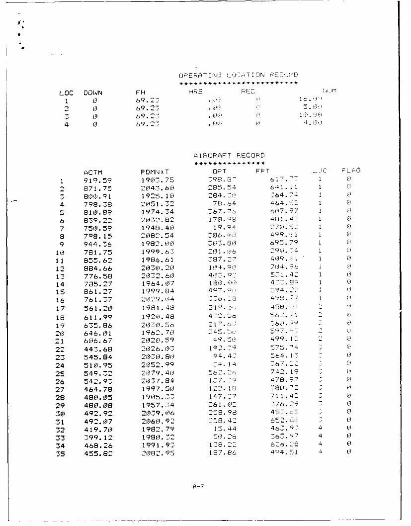
O'ERATING L'2,Z11I-ION RE(-L'E.

LOC DOWN FH HRS REC rL I

1 0 69.2" . i' 0 i-.

-. v0 69.2:' 2. . OH0 ~69.2. U01.4

4 0 69. 2. . ; 4. 0.

AIRCRAFT RECORD

ACTM FDMNX T OPT FF'T L'" FCLAG

1 919.59 1903.75 798. 6 - 17 .7- 1

2 871.75 2..... 60 285 54 641 1 4

8( 0. 91 1925.1 8.7( :-64.74 I

4 798.38 2051. 2- 2 78.b4 464.- ..

5 81 l.j. 89 1974.34 76776 6(7. 97 1 U

6 8:9.22 2..).82 178 .Q 481. 47 1

7 750. 59 1948. 40 19.94 27,f;J. 5 1

8 78. 15 2082.54 86 ,o 499. ( i 1

9 944.36 1982. 00...'. 695.7 I

10 781. 75 1999.67 20 1. 0 6 290.74 f 4

11 855.62 1986.61 :87.:7 409. U 1 1 0

12 884.66 2030.20 14. c0 704. 9, I .

13 776.58 20.2. 60 407. : 571.42 1 U

14 725.27 1964. 07 180.o, 4 7. 9'-

15 861.27 1999.84 4Q-, O , 594. ... . M.

16 761.37 2029.04 a. 4 492.

17 561. 20 1981.48 21Q. .- , 48E. '4 .

18 611.99 1920. 48 472 - 52.

19 635.86 2,30.56 217. 6! 0.20 646. 01 1962.7 ..0 24 4 5L7 L-.0

21 606. 67 2 020.59 49 5--' 499.1-' 2

22 443.68 226. - • 57•774

23 545.64 2 0-3.. 81 94. 4-. 564.1: 0

24 5 10. 95 2152. 99 4. 14 T7 . 22

25 549. 32 2079. 40 5b2. 742.19 7 jU

26 542. 93-7 2077.84 177. P9 48. 97

27 464.78 1997.5 1.18 580. -'2 e28 480. 05 1905. .7 147.77 711.42 0

29 480.08 1957.34 261.02 776.29 0

30 492. 92 23; 19. f;$6 253. 9 48-.t 9 5

31 492•. 07 21060.92 25e.42 652. GO

32 419.70 1982.79 15.44 467.9. 4 0

.33 399.12 1980.732 7.716.97 4

34 468.26 1991.97. 18. 626. 28 4 0

35 455.8 2 2018e 2.95 187.86 4Q4.51 , 0

B-7

SHIFP1Lj6 ,---HELULE

9 16 2 :.7 49 5 T

1 27 28 -4 39 9 56 47 41 - i 12 12

A 0 0 1 6 6 2 5 4 -

4

6

# OF FAILURES # OF SHIPMENTS MONTH57 57 14

CONTAINER DATA

NAME WT LIFE COST LABOR/MIN MTEOF MAINTENANI\j.

NON-REUSAB 190. 2. 25i0. 65. iKO.1 -TR I 2.04. 10. 119)9. . . 1) .20-TR P 290. 2t:. t 0.1 5. 8. 25.

SHIPPING COSTS

'5 00: _ 1 !t)). 2i : 24) :Y ,H 1 P -T I ME V.

183.75 15.80 15. 14.80 14. il 17.5, 5. ,.22. 0 15. 00 14.50 14. 0 1 "50 12. 00 1 1. ,.

00 10. fI 9. 00 8. 00C' 7. 00 b. .'i 5. I- . ,.00 6.00 5. 91 5.8 0 4. c,o 4.'3) -l 2-.

01. 5. 00 5 0 . 0000I- 9. I a. II 7. 00 5. C;'j 4. f;)i 2.

- 7lfj .. .II' ))' ..

B-8

4.

CONTAINER PFRuF M

TOTAL SPARES PROD CONTA I NER SH I F-'F' I NG FACG /UNF'AC CONTA INEF:

CONTAINERS STORAGE SHIP COST COST CoSF MAINTEN"'N

1161 B52 7t-*19 **,*-** . *-,- -( .(14. -24f. '* ,

THESE RESULTS USE CONTAINER TYPE : NON-REUSAB

AS THE PRODUCTION SHIPPING CONTAINER

**TOTAL COST OF THIS OPTION = 26B-5I.-, :)

NUMBER OF EXTRA SPARES REQUIRED =2 -'

NUMBER OF REPLACEMENT CONTAINERS = 441

# OF PROD CONTAINERS USED ALSO FOR SPAPES =

# OF CONT SHIPPED TO DEPOT FOR REUSE=

# OF CONTAINERS SHIPPED TO DEPOT P NOT USED=

CONTAINER PROGRAM

TOTAL SPARES PROD CONTAINER SHIFPING RAC ,L PNAC CONTAINE

CONTAINERS STORAGE SHIP COST COST COST MAINTENHTr

720 411 A9 .712 7 ,0 :, ,4 22 -.44_..

THESE RESULTS USE CONTAINER TYFE : I,-TRIF'

AS THE PRODUCTION SHIPPING CONTAIErI'

**TOTAL COSF OF THIS OPTION = 112 .7,

NUMBER OF EXTRA SPARES REQUIRED

NUMBER OF REPLACEMENT CONTAINERS

# OF PROD CONTAINERS USED ALSO FOR SFARES =

# OF CONT SHIPPED TO DEPOT FOR REUSE=

# OF CONTAINERS SHIPPED TO DEPOT & NOT USED-

B-9

CONTAINER F'RbH-4r-1l

TOTAL SPARES PROD CONTAINER SHIFFING FCI FNFC N NTAItJEFCONTAINERS STORAGE SHIP COST COST COST -,INTE ,.AJC-

720 411 709 72 0 ) 0 5245.4 &. 4725.

THESE RESULTS USE CONTAINER TYPE : 2-,.-TRIFAS THE PRODUCTION SHIPPING CONTAINER

**TOTAL COST OF THIS OPTION = 127S(;t5. 4K

NUMBER OF EXTRA SPARES REQUIRED = 27NUMBER OF REPLACEMENT CONTAINERS =# OF PROD CONTAINERS USED ALSO FOR SF"FES=# OF CONT SHIPPED TO DEPOT FOR REUSE=# OF CONTAINERS SHIPPED TO DEPOT & NOT U.EL=

Stop - Program terminated.

B-10

0(n - defense technical information center · 0(n simulation techn ique for ... air force packaging...

Documents