11

A. M. Sharaf, A. M. Sharaf, SMIEEESMIEEE

S. M. A. SaleemS. M. A. Saleem

Department of Electrical and Computer EngineeringDepartment of Electrical and Computer Engineering

University of New BrunswickUniversity of New Brunswick

APPLICATION OF NEURAL APPLICATION OF NEURAL NETWORKS AND WAVELET NETWORKS AND WAVELET

TRANSFORMS IN HIGH IMPEDANCE TRANSFORMS IN HIGH IMPEDANCE FAULT DETECTION IN ELECTRICAL FAULT DETECTION IN ELECTRICAL

SYSTEMSSYSTEMS

22

Introduction - High Introduction - High Impedance Fault (HIF)Impedance Fault (HIF)

Definition :Definition : A High impedance fault (HIF) or A High impedance fault (HIF) or Arc type fault is usually caused when a current Arc type fault is usually caused when a current carrying-wire or conductor inadvertently makes carrying-wire or conductor inadvertently makes a non-solid or temporary-contact with the a non-solid or temporary-contact with the ground or is temporarily short-circuited with ground or is temporarily short-circuited with another current carrying conductor through a another current carrying conductor through a high impedance mediumhigh impedance medium..

Examples of HIF-Arc fault :Examples of HIF-Arc fault :

AA cable lying and touching the ground. cable lying and touching the ground.

A tree branch touching one or two power A tree branch touching one or two power cables.cables.

33

Research Objectives and MethodsResearch Objectives and Methods

1.1. Investigate the best selection of mother Investigate the best selection of mother wavelet, which best depicts the pattern of the wavelet, which best depicts the pattern of the High Impedance arc type fault for the High Impedance arc type fault for the Wavelets based fault detection.Wavelets based fault detection.

2. Investigate the level of Fault diagnostic signal 2. Investigate the level of Fault diagnostic signal decomposition, which would yield good decomposition, which would yield good characteristic patterns for arc type HIF using characteristic patterns for arc type HIF using the Wavelets based relaying scheme.the Wavelets based relaying scheme.

44

Research Objectives and Methods Research Objectives and Methods - cont.- cont.

3. Optimize the Neural Network architecture vis-à-3. Optimize the Neural Network architecture vis-à-vis the number of hidden layers, activation vis the number of hidden layers, activation functions and the number of neurons for the functions and the number of neurons for the Wavelets based fault detection.Wavelets based fault detection.

4. Investigate an effective training algorithm to be 4. Investigate an effective training algorithm to be adopted for training the Neural Network for the adopted for training the Neural Network for the Wavelets based fault detection.Wavelets based fault detection.

5. Design and validate a Neural Network based 5. Design and validate a Neural Network based relaying scheme structure in Matlab/ Simulink relaying scheme structure in Matlab/ Simulink for the Wavelets based fault detection scheme.for the Wavelets based fault detection scheme.

55

Matlab / Simulink HIF ModelMatlab / Simulink HIF Model

The current-dependant-resistance nonlinearity is The current-dependant-resistance nonlinearity is incorporated by a simple current dependent nonlinear incorporated by a simple current dependent nonlinear resistance ‘resistance ‘RRff’ developed by Dr. Sharaf and defined as,’ developed by Dr. Sharaf and defined as,

010

f

ffff i

iRRR

where Rf0 = 100 Ω, Rf1 = 50 to 150 Ω, if0 = 70 A, α = 0.3 to 0.7, β = 2, Rf is usually high.

Arc-current extinction and re-ignition nonlinearity is incorporated by using a dead zone nonlinear function.

Arc current asymmetry is incorporated by modifying the ‘start’ and ‘end’ of the dead zone function such that the HIF current’s positive half cycle is greater than the negative half cycle.

Eq (1)

66

Radial Electric Utility Distribution Radial Electric Utility Distribution System - Single Line DiagramSystem - Single Line Diagram

Figure 1. Single Line Diagram of a Radial Transmission / Utilization System (25 kV) with fault location (x). PT, CT are located at feeder bus Va.

Vs = 25 kV (L-L), Ls = 7 mH, Rs = 0.7 Ω, Rline = 0.25 Ω / km, Lline = 0.99472 mH / km, Cline = 0.01117 μF / km, l = 25 km, x = 0 to 25 km, Rload = 72 to 144 Ω, Lload = 0.1719 to 0.3438 H.

77

Radial Electric Utility Distribution Radial Electric Utility Distribution System - Per phase Equivalent System - Per phase Equivalent

DiagramDiagram

Figure 2. Simple per phase equivalent HIF – Arc fault lumped parameter circuit for Radial Distribution System used in digital simulations (developed by Dr. Sharaf).

88

Radial Electric Utility Distribution Radial Electric Utility Distribution System - Functional Block DiagramSystem - Functional Block Diagram

Figure 3. Functional block model of HIF – Arc fault in a Radial Distribution System.

Va'

Ia'

4Out4

3Out3

2Out2

1Out1-K-

x*Cline

1

den(s)x*(Lline + Rline)

Source

f(u)

Rf Product2

Product1

Product

-K-

PT1

den(s)Ls + Rs

1

den(s)Lload + Rload

-K-

Lf

1/s

Integrator1

1/s

Integrator

du/dt

Derivative

Dead Zone

-K-

CT

1

den(s)(l-x)*(Lline + Rline)

-K-

(l-x)*(Cline) sig4

sig3

sig2

sig1

Is

Vs Va

Va

Vf

Vf

Vf

IaIa

Ia

Ib

Ib

Ib

IfIf VRf

VLf

Vb

Vb

VbPa'

Pa'

Pa'

Ya'

Ya'Ya'

Va'

Va'

Va'

Va'

99

Radial Electric Utility Distribution Radial Electric Utility Distribution System - Functional Block DiagramSystem - Functional Block Diagram

Figure 4. Dialog box for High impedance – Arc fault model for Radial Distribution System.

1010

Digital Simulation - Radial SystemDigital Simulation - Radial System

TABLE I

TRAINING AND VALIDATION DATA FOR RADIAL AC SYSTEM

(50 CASE STUDIES)

H = HIF, L = Linear fault, B = Bolted fault, N = Normal operation, TR =Training, TS = Testing, x = distance to fault, 1) Ref. Eq. (1), 2) Ref. Figure 1.

Case Fault x a1) ß1)Rf1

1) Lf2) Rload

2) Lload2) Converter

No. Type Load1 H 2.5 0.3 2.0 50.0 0.0010 72.0 0.2 No2 H 2.5 0.7 2.0 100.0 0.0040 110.0 0.25 No3 H 20.0 0.4 2.0 75.0 0.0020 85.0 0.3 No4 H 5.0 0.4 2.0 75.0 0.0050 100.0 0.25 No5 H 15.0 0.4 2.0 50.0 0.0030 120.0 0.18 No6 H 15.0 0.5 2.0 55.0 0.0010 100.0 0.34 No7 H 2.5 0.4 2.0 85.0 0.0025 140.0 0.2 No8 H 15.0 0.4 2.0 80.0 0.0025 120.0 0.18 No9 H 2.5 0.7 2.0 50.0 0.0045 140.0 0.3 No

10 L 2.5 N.A. N.A. 100.0 0.0020 75.0 0.2 No11 L 15.0 N.A. N.A. 150.0 0.0010 100.0 0.3 No12 L 20.0 N.A. N.A. 200.0 0.0050 140.0 0.17 No13 L 15.0 N.A. N.A. 150.0 0.0030 80.0 0.25 No14 L 5.0 N.A. N.A. 100.0 0.0050 100.0 0.3 No15 L 20.0 N.A. N.A. 150.0 0.0010 140.0 0.28 No16 B 2.5 N.A. N.A. N.A. N.A. 100.0 0.3 No17 B 20.0 N.A. N.A. N.A. N.A. 75.0 0.2 No18 B 15.0 N.A. N.A. N.A. N.A. 100.0 0.25 No19 B 10.0 N.A. N.A. N.A. N.A. 80.0 0.3 No20 B 2.5 N.A. N.A. N.A. N.A. 140.0 0.18 No21 N N.A. N.A. N.A. N.A. N.A. 80 0.2 No22 N N.A. N.A. N.A. N.A. N.A. 100.0 0.3 No23 N N.A. N.A. N.A. N.A. N.A. 140.0 0.25 No24 N N.A. N.A. N.A. N.A. N.A. 75.0 0.2 No25 N N.A. N.A. N.A. N.A. N.A. 120.0 0.18 No26 H 2.5 0.3 2.0 50.0 0.0010 72.0 0.2 Yes27 H 2.5 0.7 2.0 100.0 0.0040 110.0 0.25 Yes28 H 20.0 0.4 2.0 75.0 0.0020 85.0 0.3 Yes29 H 5.0 0.4 2.0 75.0 0.0050 100.0 0.25 Yes30 H 15.0 0.4 2.0 50.0 0.0030 120.0 0.18 Yes31 H 15.0 0.5 2.0 55.0 0.0010 100.0 0.34 Yes32 H 2.5 0.4 2.0 85.0 0.0025 140.0 0.2 Yes33 H 15.0 0.4 2.0 80.0 0.0025 120.0 0.18 Yes34 H 2.5 0.7 2.0 50.0 0.0045 140.0 0.3 Yes35 L 2.5 N.A. N.A. 100.0 0.0020 75.0 0.2 Yes36 L 15.0 N.A. N.A. 150.0 0.0010 100.0 0.3 Yes37 L 20.0 N.A. N.A. 200.0 0.0050 140.0 0.17 Yes38 L 15.0 N.A. N.A. 150.0 0.0030 80.0 0.25 Yes39 L 5.0 N.A. N.A. 100.0 0.0050 100.0 0.3 Yes40 L 20.0 N.A. N.A. 150.0 0.0010 140.0 0.28 Yes41 B 2.5 N.A. N.A. N.A. N.A. 100.0 0.3 Yes42 B 20.0 N.A. N.A. N.A. N.A. 75.0 0.2 Yes43 B 15.0 N.A. N.A. N.A. N.A. 100.0 0.25 Yes44 B 10.0 N.A. N.A. N.A. N.A. 80.0 0.3 Yes45 B 2.5 N.A. N.A. N.A. N.A. 140.0 0.18 Yes46 N N.A. N.A. N.A. N.A. N.A. 80 0.2 Yes47 N N.A. N.A. N.A. N.A. N.A. 100.0 0.3 Yes48 N N.A. N.A. N.A. N.A. N.A. 140.0 0.25 Yes49 N N.A. N.A. N.A. N.A. N.A. 75.0 0.2 Yes50 N N.A. N.A. N.A. N.A. N.A. 120.0 0.18 Yes

1111

Wavelets TransformWavelets Transform

FFT has its limitations. The biggest drawback of FFT has its limitations. The biggest drawback of FFT is that it provides only the frequency spectra FFT is that it provides only the frequency spectra information of the input time domain signal. information of the input time domain signal.

Wavelets provide similar information as provided Wavelets provide similar information as provided by the FFT plus additional time information.by the FFT plus additional time information.

In wavelets, small windows are used to capture In wavelets, small windows are used to capture the high frequency information and large windows the high frequency information and large windows are used to capture the low frequency information.are used to capture the low frequency information.

1212

Wavelets TransformWavelets Transform

Wavelets Transforms do not employ sinusoids to Wavelets Transforms do not employ sinusoids to extract the frequency information from the input time extract the frequency information from the input time signal. Instead of sinusoids, wavelets transforms signal. Instead of sinusoids, wavelets transforms utilize ‘mother wavelets’.utilize ‘mother wavelets’.

The Wavelet Transform measures the correlation The Wavelet Transform measures the correlation between the input signal and scaled and translated between the input signal and scaled and translated version of the ‘Mother Wavelet’. version of the ‘Mother Wavelet’.

DWT is obtained by using a multistage filter with the DWT is obtained by using a multistage filter with the mother wavelet as the lowpass filter mother wavelet as the lowpass filter l l ((nn) and its dual ) and its dual as the highpass filter as the highpass filter h h ((nn). The output of the highpass ). The output of the highpass filter gives the detailed version of the high-frequency filter gives the detailed version of the high-frequency component of the signal. The low-frequency component of the signal. The low-frequency component is split to get the other details of the input component is split to get the other details of the input signal.signal.

1313

Wavelets Packet AnalysisWavelets Packet Analysis

Another method of Discrete Wavelets Transform, Another method of Discrete Wavelets Transform, which is employed in this thesis, is the Wavelet which is employed in this thesis, is the Wavelet Packet Analysis. In Wavelet Packet Analysis, the Packet Analysis. In Wavelet Packet Analysis, the details as well as the approximations are split as details as well as the approximations are split as opposed to Wavelet Analysis where a signal is opposed to Wavelet Analysis where a signal is split into an approximation and a detail and then split into an approximation and a detail and then only the approximation is split into next level only the approximation is split into next level approximation and detail. approximation and detail.

1414

Wavelets Packet AnalysisWavelets Packet Analysis

Figure 5. Decomposition of signal ‘S’ using Wavelet Packet Analysis. Note thatApproximation and Details are further decomposed as compared to Simple WaveletAnalysis, Figure 2. 3 where only the Approximation is further decomposed. ‘A’ and‘D’ stand for Approximation and Detail respectively.

1515

Why use Wavelets Transform for Why use Wavelets Transform for HIF - Arc Fault Detection ?HIF - Arc Fault Detection ?

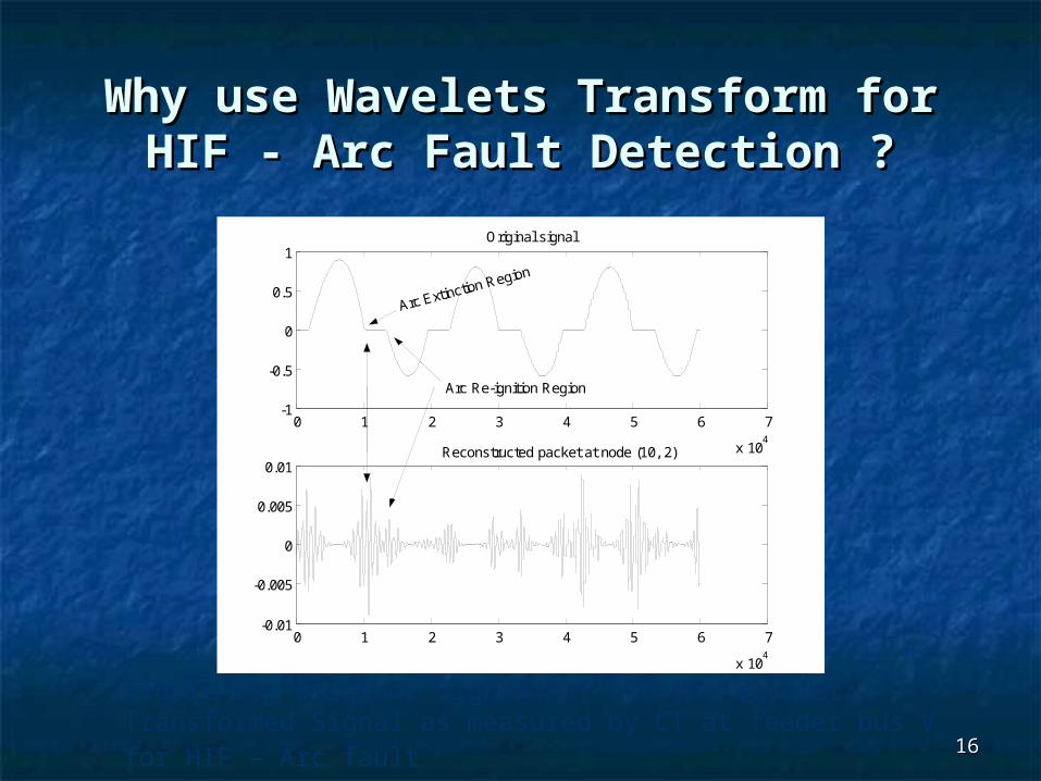
The fault current has discontinuities due to fault The fault current has discontinuities due to fault current temporary extinction and re-ignition current temporary extinction and re-ignition phenomena. This attribute is used in the phenomena. This attribute is used in the Wavelet detection method.Wavelet detection method.

However, in the case of occurrence of a HIF - Arc However, in the case of occurrence of a HIF - Arc fault, the magnitude of feeder current at the fault, the magnitude of feeder current at the substation is relatively much higher than the HIF substation is relatively much higher than the HIF - Arc fault current. As a result the feeder current - Arc fault current. As a result the feeder current would be nearly sinusoidal and the ANN might would be nearly sinusoidal and the ANN might not be able to distinguish between a faulty not be able to distinguish between a faulty feeder current and a healthy feeder current.feeder current and a healthy feeder current.

1616

Why use Wavelets Transform for Why use Wavelets Transform for HIF - Arc Fault Detection ?HIF - Arc Fault Detection ?

Figure 6. Original Signal I(t) and the Wavelet Transformed Signal as measured by CT at feeder bus Va for HIF – Arc fault

0 1 2 3 4 5 6 7

x 104

-1

-0.5

0

0.5

1Original signal

0 1 2 3 4 5 6 7

x 104

-0.01

-0.005

0

0.005

0.01Reconstructed packet at node (10, 2)

Arc Extinction Region

Arc Re-ignition Region

1717

Wavelets and Artificial Neural Wavelets and Artificial Neural Networks in HIF - Arc Fault Networks in HIF - Arc Fault Detection Relaying SchemeDetection Relaying Scheme

The instantaneous value of the feeder current The instantaneous value of the feeder current i i ((t t ) ) at the feeder substation bus are obtained.at the feeder substation bus are obtained.

i i ((t t ) is transformed into the Wavelet domain using ) is transformed into the Wavelet domain using Wavelet Packet Analysis.Wavelet Packet Analysis.

The signal is reconstructed at each node and The signal is reconstructed at each node and analyzed to select the ‘best reconstruction’ from analyzed to select the ‘best reconstruction’ from the signal decomposition tree also called Wavelet the signal decomposition tree also called Wavelet Packet Tree (WPT).Packet Tree (WPT).

After many iterations, node (10, 2) and After many iterations, node (10, 2) and Daubechies4 Mother Wavelet (db4) was found to Daubechies4 Mother Wavelet (db4) was found to provide the best ‘diagnostic vector’.provide the best ‘diagnostic vector’.

1818

Wavelets and Artificial Neural Wavelets and Artificial Neural Networks in HIF - Arc Fault Networks in HIF - Arc Fault Detection Relaying SchemeDetection Relaying Scheme

Case RMS I(10,2) RMS I(10,2) RMS I(10,2) RMS I(10,2)No. 0 <= t <= T/4 T/4 < t <= T/2 T/2 < t <= 3T/4 3T/4 < t <= T

(A) (A) (A) (A)1 0.018998 0.009651 0.019503 0.0103872 0.023753 0.010090 0.020648 0.0126603 0.013549 0.004837 0.021988 0.0102644 0.014120 0.007212 0.025118 0.0131425 0.006704 0.007591 0.035373 0.0137426 0.011150 0.007888 0.036909 0.0143397 0.020952 0.009498 0.019845 0.0113558 0.007905 0.007882 0.036455 0.0141289 0.022399 0.009556 0.018415 0.011970

10 0.005768 0.006551 0.004361 0.00345611 0.004622 0.005211 0.002598 0.00148012 0.004164 0.004691 0.002042 0.00138613 0.004179 0.004966 0.002476 0.00136914 0.005191 0.005741 0.003510 0.00285515 0.004178 0.004554 0.002023 0.00132916 0.003519 0.003321 0.003464 0.00335417 0.001037 0.001198 0.001023 0.00120418 0.001302 0.001464 0.001285 0.00148019 0.001746 0.001897 0.001722 0.00191220 0.003519 0.003321 0.003464 0.00335421 0.005931 0.004872 0.004224 0.00687522 0.006307 0.005224 0.004530 0.00731023 0.006171 0.005111 0.004435 0.00709524 0.005923 0.004857 0.004217 0.00688525 0.005843 0.004820 0.004182 0.00669426 0.032025 0.019766 0.046516 0.02021327 0.038528 0.022693 0.049433 0.02209028 0.023752 0.012294 0.012986 0.00598729 0.040702 0.020886 0.059026 0.02260730 0.015920 0.011395 0.020746 0.00777531 0.016274 0.011133 0.022173 0.00805932 0.034137 0.020889 0.046992 0.02077433 0.016728 0.011757 0.021135 0.00794134 0.037489 0.022487 0.050700 0.02222135 0.041638 0.018659 0.056038 0.01720136 0.026121 0.011117 0.037494 0.01247637 0.025269 0.010189 0.033834 0.01078838 0.026286 0.010700 0.035726 0.01166339 0.036203 0.015651 0.048071 0.01472940 0.021095 0.009469 0.031716 0.01118541 0.003519 0.003321 0.003464 0.00335442 0.001037 0.001198 0.001023 0.00120443 0.001302 0.001464 0.001285 0.00148044 0.001746 0.001897 0.001722 0.00191245 0.003519 0.003321 0.003464 0.00335446 0.054337 0.018615 0.049037 0.01584347 0.057664 0.019849 0.051950 0.01676848 0.056290 0.019382 0.050874 0.01639849 0.054337 0.018607 0.049016 0.01584350 0.053334 0.018303 0.048354 0.015573

TABLE II

FEATURE VECTORS FOR TRAINING, TESTING AND CROSS-VALIDATING THE ELMAN ANN FOR RADIAL ELECTRIC UTILITY FEEDER DISTRIBU-TION SYSTEM

1919

Artificial Neural Network Design Artificial Neural Network Design Using Recurrent Network- Using Recurrent Network-

ArchitectureArchitecture

Elman Recurrent Network.Elman Recurrent Network. One hidden layer.One hidden layer. 10 neurons in the hidden layer.10 neurons in the hidden layer. 2 neuron in the output layer.2 neuron in the output layer. The activation function was tan-sigmoid for the The activation function was tan-sigmoid for the

hidden layer and pure-linear for the output hidden layer and pure-linear for the output layer.layer.

2020

Artificial Neural Network Design - Artificial Neural Network Design - Training AlgorithmsTraining Algorithms

1) Variable Learning Rate Backpropagation (traingdx)*1) Variable Learning Rate Backpropagation (traingdx)* 2) Resilient Backpropagation (trainrp)2) Resilient Backpropagation (trainrp) 3) BFGS Quasi-Newton (trainbfg)3) BFGS Quasi-Newton (trainbfg) 4) Scaled Conjugate Gradient (trainscg)4) Scaled Conjugate Gradient (trainscg) 5) Polak-Ribiére Conjugate Gradient (traincgp)5) Polak-Ribiére Conjugate Gradient (traincgp) 6) Fletcher-Powell Conjugate Gradient (traincg)6) Fletcher-Powell Conjugate Gradient (traincg)

Variable Learning Rate Backpropagation (traingdx) Variable Learning Rate Backpropagation (traingdx) algorithm* (number 1 above) was the fastest algorithm* (number 1 above) was the fastest algorithm in all cases.algorithm in all cases.

2121

High Impedance - Arc Fault High Impedance - Arc Fault Detection and Relaying SchemeDetection and Relaying Scheme

Module-1: Input BlockModule-1: Input Block Module-2: Signal Processing BlockModule-2: Signal Processing Block Module-3: ANN BlockModule-3: ANN Block Module-4: Output Logical BlockModule-4: Output Logical Block

Figure 11. Relay 2. FFT Hyper-plane ANN Based HIF – Arc fault Detection Scheme (developed by Dr. Sharaf ).

2222

Conclusion - Research Extensions Conclusion - Research Extensions and Recommendationsand Recommendations

The thesis developed and validated two novel ANN-The thesis developed and validated two novel ANN-Based HIF - Arc fault relaying schemes based on Dr. Based HIF - Arc fault relaying schemes based on Dr. Sharaf’s Feature Vector Transformations.Sharaf’s Feature Vector Transformations.

Develop a Multi-tier detection approach using a Develop a Multi-tier detection approach using a combination of High impedance arcing type fault combination of High impedance arcing type fault detection methods.detection methods.

Rule-based identification and activation procedure Rule-based identification and activation procedure be incorporated into any effective and robust HIF - be incorporated into any effective and robust HIF - Arc fault relaying scheme, so that it could Arc fault relaying scheme, so that it could accurately initiate the Trip / Isolate signal to the accurately initiate the Trip / Isolate signal to the Circuit Breaker / Contactor / Oil Circuit Breaker as Circuit Breaker / Contactor / Oil Circuit Breaker as well as initiate the required Alarm and Fault-well as initiate the required Alarm and Fault-Recorder Activation.Recorder Activation.

2323

Conclusion - Research Extensions Conclusion - Research Extensions and Recommendations - cont.and Recommendations - cont.

Extend the concept of the full n-dimensional hyper-Extend the concept of the full n-dimensional hyper-plane / fault-phase / phase portraits degeneration plane / fault-phase / phase portraits degeneration recently developed by Dr. Sharaf, where new recently developed by Dr. Sharaf, where new synthesized / transformed multi-input signal hyper-synthesized / transformed multi-input signal hyper-vector called the Anomaly-Graphic Feature (AGF) vector called the Anomaly-Graphic Feature (AGF) vector is traced in the 2-dimensional, 3-dimensional vector is traced in the 2-dimensional, 3-dimensional trajectory or any hyper-plane. The trajectory’s trajectory or any hyper-plane. The trajectory’s degenerative shape and temporal phase portrait degenerative shape and temporal phase portrait pattern can be used by a graphic Object-detection pattern can be used by a graphic Object-detection software as indicative of HIF – Arc Faults.software as indicative of HIF – Arc Faults.

Design a Radio frequency (RF) HIF – Arc fault Design a Radio frequency (RF) HIF – Arc fault detection scheme using active successive detection scheme using active successive estimation and abduction rules.estimation and abduction rules.

2424

Thank youThank you

Questions PleaseQuestions Please