1. ac fundamentals - city university of new york fundamentals.pdf · 1. ac fundamentals caution: in...

1

Syed A. Rizvi ENS 441/ELT 437

1. AC Fundamentals

Caution: In these experiments high voltages are involved, which could be harmful or fatal if one

is exposed to them. Adhere to electrical safety rule at all times. Make sure that all of your

connections are correct before turning on the power.

In 1831 Michael Faraday discovered the fundamental relationship between the voltage and magnetic

flux in a circuit. This relationship is now known as Faraday’s law of electromagnetic induction, which

states:

If the flux linking a conductor forming a loop changes with time, a voltage is induced at its terminal.

The magnitude of the induced voltage is proportional to the rate of change in the magnetic flux.

Mathematically the law is stated as follows:

𝐸 = 𝑁

𝑑∅

𝑑𝑡 (1)

where,

E = induced voltage (in volts)

N = number of turns in the conductor

Φ = Flux linking the conductor

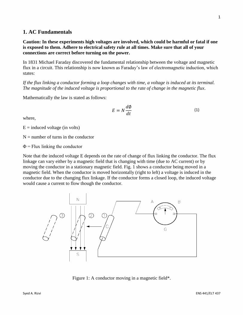
Note that the induced voltage E depends on the rate of change of flux linking the conductor. The flux

linkage can vary either by a magnetic field that is changing with time (due to AC current) or by

moving the conductor in a stationary magnetic field. Fig. 1 shows a conductor being moved in a

magnetic field. When the conductor is moved horizontally (right to left) a voltage is induced in the

conductor due to the changing flux linkage. If the conductor forms a closed loop, the induced voltage

would cause a current to flow though the conductor.

Figure 1: A conductor moving in a magnetic field*.

2


Note that the polarity of the induced voltage and the direction of the current through the conductor

would reverse when the conductor is moved back from left to right. Furthermore, no voltage would be

induced if the conductor in Fig. 1 is moved vertically because the flux through the conductor would not

change in the vertical movement. Alternatively, the induced voltage can be expressed as:

𝐸 = 𝐵𝑙𝑣 (2)

where,

𝐵 = ∅

𝐴 is the flux density (in Weber/meter

2: Wb/m

2 or Telsa: T)

l = active length of the conductor in the magnetic field (m)

v = relative speed of the conductor (m/s)

A current carrying conductor, when placed in a magnetic field, experiences a force known as

electromagnetic force (also called Lorentz force). This force is the basis of the operation of the

electrical motors and generators. The maximum force is exerted on the current carrying conductor

when it is perpendicular to the magnetic field and it is zero when the conductor is parallel to the field.

Mathematically, electromagnetic force can be expressed as:

𝐹 = 𝐵𝑙𝐼 (3)

where,

F = force exerted on the conductor (in Newton: N)

B =flux density (T)

l = active length of the conductor (m)

I = current carried by the conductor (A)

Single Phase AC Generator

There are two kinds of sources of electrical power:

(1) Direct current or voltage source (DC source) in which the current and voltage remains constant

over time.

(2) Alternating current or voltage source (AC source) in which the current or voltage constantly

changes with time. The voltage of the electrical power source that we use in our homes or

offices (line voltage) is a sinusoidal signal that goes through a complete cycle 60 times in one

second. In this section we will discuss how single phase AC voltage is generated.

Figure 2 shows a conductor placed in a magnetic field. A voltage is induced between its terminals

(x, y) due to the change in flux linkage when the conductor is rotated in the magnetic field. The

change in flux linkage is at its minimum when the conductor is moving parallel to the field and it is

at its maximum when the conductor is moving perpendicular to the magnetic field. In a half

3


rotation, the conductor moves from being parallel to the field to being perpendicular to the field

and eventually moving back to being parallel to the field. Accordingly, the induced voltage

increases from zero to its maximum value and then back to zero at the end of the half rotation.

Figure 2: A rotating conductor in a magnetic field*.

Fig. 3 shows the changes in the induced voltage as the conductor rotates in the magnetic field.

During the second half of the rotation the flux linkage changes through the conductor the same way

as before; however, it induces the voltage with the opposite polarity because the position of the

conductors is now reversed. Due to the shape of the poles and the rotary motion of the conductor

the induced voltage turns out to be a sine wave.

Figure 3: Induced voltage vs. rotation of the conductor*.

4


The frequency of the induced voltage depends on the number of rotations completed in one second

as well as the number of poles in the generator. For the two-pole generator shown in Fig 2, a

rotational speed of 60 revolutions per second (3600 rpm) would result in an induced voltage with a

frequency of 60 Hz. The induced voltage goes through one peak to another peak in the opposite

direction as the conductor is swept through the North (N) and the South (S) poles, respectively. For

the two-pole generator in Fig 2, the frequency of the induced voltage is the same as the rotational

speed of the generator. In general, the frequency of the induced voltage is given by

𝑓 =

𝑛 × 𝑝

120 (4)

where,

f = frequency of the induced voltage (Hz)

n = rotational speed of the conductor (rpm)

p = number of poles in the generator.

Example: A single phase generator has eight poles and it generates voltage at 60 Hz. What is the

speed of the generator (in rpm)?

Solution: Use the Eq. (4) to calculate the speed of the generator.

Frequency of the induced voltage = f = 60 Hz

Number of poles = p = 8

Generator speed = n = 𝑓×120

𝑝=

60×120

8 = 900 rpm

Instantaneous and Effective Values of AC Voltage and Current

Figure41 show a graphical representation of AC voltage. The time taken to complete one cycle is

called “time period,” or simply “period” of the signal (“T’ in Fig. 4). The number of cycles

completed in one second is called “frequency.” The unit of frequency is cycles/second or Hertz

(Hz). The line voltage has a frequency of 60 Hz. The frequency “f” and the period “T” of a signal

are related by the following equation:

𝑓 =

1

𝑇 (5)

The frequency of a signal is also sometimes described in terms of the angular frequency “ω” (in

radians/second). The frequency “f” of a signal and its angular frequency “ω” are related by the

following equation:

𝜔 = 2 𝜋𝑓 (6)

5


Figure 4: AC voltage.

The AC voltage, V(t), is mathematically described as:

𝑉(𝑡) = 𝑉𝑝 𝑆𝑖𝑛 𝜔𝑡

However, a more meaningful measure of AC quantities is their “root-mean-square” (RMS) value.

Assignment 1.1: Show that:

𝐴𝑉𝐸[𝑉(𝑡)] =1

𝑇∫ 𝑉𝑝 𝑆𝑖𝑛 𝜔𝑡 = 0

𝑇

0

And

𝑅𝑀𝑆[𝑉(𝑡)] = √1

𝑇∫ 𝑉𝑝

2𝑠𝑖𝑛2𝜔𝑡 𝑇

0=

𝑉𝑝

√2

Output Power of a Single Phase Generator

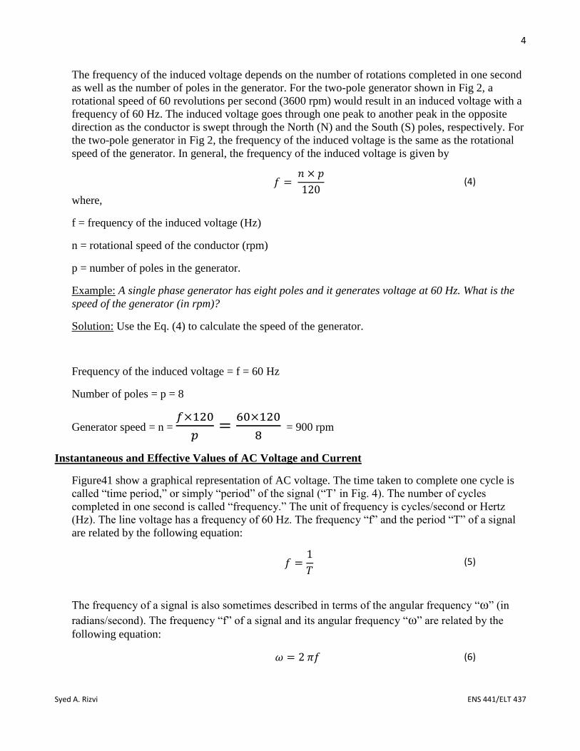
Figure 5 shows the instantaneous voltage, current, and power (which is a product of instantaneous

voltage and current) of a single phase generator. In Fig. 5 the voltage and current are in phase and,

therefore, the instantaneous power is positive throughout the whole cycle. Note that the output

power of a single phase generator is not constant. Instead, it is pulsating at a frequency that is twice

the frequency of the induced voltage. However, most of the mechanical energy sources that are

used to create the rotary motion of the conductors (or the magnetic field) in an AC generator

provide a constant mechanical power. This imbalance in the constant mechanical power at the

input and the pulsating electrical power at the output of the generator results in machine vibrations

and makes single phase generator undesirable.

6


Figure 5: Instantaneous voltage, current, and power of a single phase AC generator.

Assignment 1.2: Study of RLC circuits with AC voltage source.

Components needed:

Resistor 10 Ω (2)

Capacitor 35 µF (1), 20 µF (1)

Inductor 39 mH (2), 10 mH (5), 100 mH (3)

Note: Measure the voltage by connecting the Voltmeter in parallel and measure the current by

connecting the Ammeter in the series.

A. Parallel RLC Circuit

1. Build the circuit in Fig. 6 with ZL = 78 mH (2x39), ZR = 20 Ω, and ZC = 55 µF.

2. Use a 30V AC source and measure the currents I, IL, IR, and IC. Apply KCL to the circuit (I = IL

+ IR + IC). Explain your results.

3. Increase ZL to128mHin 10mH increments and record all the currents.

4. Increase ZLto428 mH in 100 mH increments and record all the currents.

7


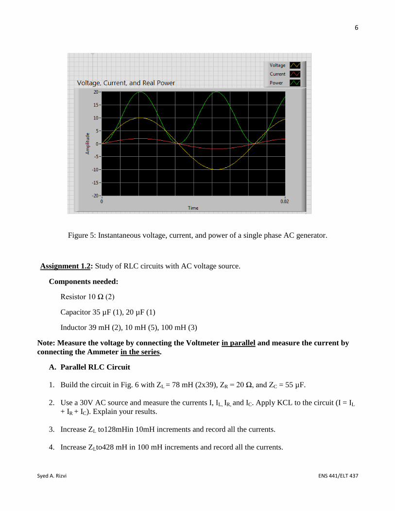
5. Plot I, IL, IR, and ICvs ZL. Note down the value of ZL where I and IR are closest to each other.

What do you observe about IL and IC at that value of ZL? Explain your results.

Figure 6: Parallel RLC circuit.

B. Series RLC Circuit

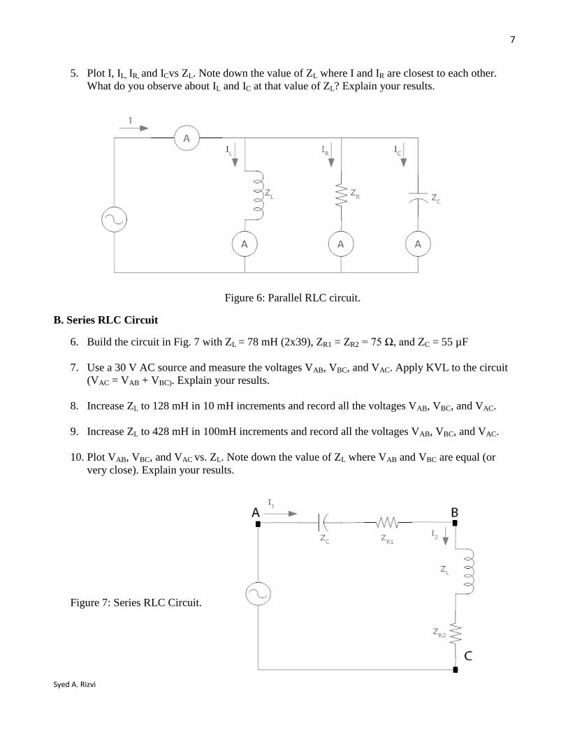
6. Build the circuit in Fig. 7 with ZL = 78 mH (2x39), ZR1 = ZR2 = 75 Ω, and ZC = 55 µF

7. Use a 30 V AC source and measure the voltages VAB, VBC, and VAC. Apply KVL to the circuit

(VAC = VAB + VBC). Explain your results.

8. Increase ZL to 128 mH in 10 mH increments and record all the voltages VAB, VBC, and VAC.

9. Increase ZL to 428 mH in 100mH increments and record all the voltages VAB, VBC, and VAC.

10. Plot VAB, VBC, and VAC vs. ZL. Note down the value of ZL where VAB and VBC are equal (or

very close). Explain your results.

Figure 7: Series RLC Circuit.

8


2. Impedance and Phase

AC quantities are identified with two parameters: magnitude and phase (angle). Accordingly, AC

quantities such voltage, current, power, etc. are expressed as complex numbers such as

A + j B (7)

Where, A and B are called the real and reactive components of that quantity. This form of a complex

number is called “rectangular” form. Alternatively, each quantity can also be expressed with the

magnitude and associated phase (angle in electrical degrees). That is, for A + j B

𝑀𝑎𝑔𝑛𝑖𝑡𝑢𝑑𝑒 = |𝑀| = √𝐴2 + 𝐵2 (8)

𝑃ℎ𝑎𝑠𝑒 = ∅ = tan−1(

𝐵

𝐴) (9)

When the magnitude and the phase of an electrical quantity are known, it is expressed in the “polar”

form of a complex number as follows:

|𝑀|⟨𝜙 = √𝐴2 + 𝐵2 ⟨tan−1(

𝐵

𝐴) (10)

If the magnitude |M| and the phase angle Φ of an AC quantity are known, the real and reactive

components of the AC quantity (A and B in Eq. 7) can be computed as follows:

𝐴 = |𝑀| × cos 𝜙 (11) 𝐵 = |𝑀| × sin 𝜙 (12)

Figure 6 shows the relationship between the polar and rectangular form of AC quantities.

Figure 6: Relationship between the polar and rectangular AC quantities.

9


Rules for manipulating complex numbers:

1. Addition or subtraction

a. Use rectangular form

b. The real part of one complex number can only be added to (or subtracted from) the real

part of another complex number.

c. The imaginary (reactive) part of a complex number can only be added to (or subtracted

from) the imaginary (reactive) part of another complex number.

2. Multiplication or division

a. Use polar form

b. Multiplication: The magnitudes of the complex numbers are multiplied and their

corresponding angles are added together.

c. Division: The magnitude of the complex number in the numerator is divided by the

magnitude of the complex number in the denominator. The angle of the complex

number in the denominator is subtracted from the angle of the complex number in the

numerator.

AC Voltage-Current Relationships for Resistance, Inductance, and Capacitance

If an AC voltage 𝑉(𝑡) = 𝑉𝑝 𝑆𝑖𝑛 𝜔𝑡 is applied across a resistor R, the current IR though the resistor is

given by

𝐼𝑅 =𝑉𝑃

𝑅𝑆𝑖𝑛 𝜔𝑡. (13)

Note the current though a resistor is in-phase with the applied voltage.

If an AC voltage 𝑉(𝑡) = 𝑉𝑝 𝑆𝑖𝑛 𝜔𝑡 is applied across an inductor of inductance L, the current IL

though the inductor is given by

𝐼𝐿 =

1

𝐿∫ 𝑉(𝑡)𝑑𝑡 (14)

or

𝐼𝐿 =

𝑉𝑝

𝐿∫ 𝑆𝑖𝑛 𝜔𝑡 𝑑𝑡. (15)

After integrating the R.H.S. we get

𝐼𝐿 =

𝑉𝑝

𝜔𝐿cos 𝜔𝑡 =

𝑉𝑝

𝜔𝐿sin (𝜔𝑡 − 900

) . (16)

10


Note the current through an inductor is out-of-phase with the applied voltage and it lags the applied

voltage by 900. The figure shows the voltage-current relationship of an inductor. The quantity “𝜔𝐿" is

called the impedance of the inductor. We will represent the impedance of an inductor by Xl. Accordingly,

𝑋𝑙 = 𝜔𝐿 (17)

and, therefore,

𝐼𝐿 =

𝑉𝑝

𝑋𝑙sin (𝜔𝑡 − 900

) . (18)

Figure 7: (a) Instantaneous voltage and current for an inductor. (b) Phasor diagram*.

If an AC voltage 𝑉(𝑡) = 𝑉𝑝 𝑆𝑖𝑛 𝜔𝑡 is applied across a capacitor of capacitance C farads, the current

IC though the capacitor is given by

𝐼𝐶 = 𝐶

𝑑𝑉(𝑡)

𝑑𝑡 (19)

or

11


𝐼𝐶 = 𝐶 𝑉𝑝

𝑑

𝑑𝑡𝑆𝑖𝑛 𝜔𝑡. (20)

After differentiating the R.H.S. we get

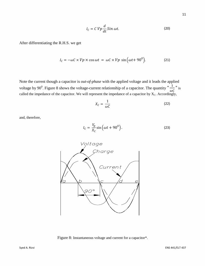
𝐼𝐶 = −𝜔𝐶 × 𝑉𝑝 × cos 𝜔𝑡 = 𝜔𝐶 × 𝑉𝑝 sin (𝜔𝑡+ 900). (21)

Note the current though a capacitor is out-of-phase with the applied voltage and it leads the applied

voltage by 900. Figure 8 shows the voltage-current relationship of a capacitor. The quantity "

1

𝜔𝐶" is

called the impedance of the capacitor. We will represent the impedance of a capacitor by XC. Accordingly,

𝑋𝐶 =

1

𝜔𝐶 (22)

and, therefore,

𝐼𝐶 =

𝑉𝑝

𝑋𝐶sin (𝜔𝑡 + 900

) . (23)

Figure 8: Instantaneous voltage and current for a capacitor*.

12


Impedance:

In AC analysis, resistance, inductance, and capacitance are represented as part of the “generalized

impedance” (or simply impedance) in the circuit and are expressed as complex numbers. The

resistance constitutes the real part of the impedance and the inductance or capacitance constitutes

the reactive (imaginary) part of the impedance. The unit for impedance is the ohm (Ω). The

impedance Z can be expressed either in the rectangular or polar form just like any other AC

quantity (voltage, current, power etc.). The impedance in rectangular form can be expressed as:

𝑍 = 𝑅 ± 𝑗𝑋

The reactive part is positive (+j) if the resultant reactance is inductive in nature and it is negative (-

j) if the resultant reactance is capacitive in nature. Alternatively,

𝑍 = 𝑅 + 𝑗𝑋𝑙

or

𝑍 = 𝑅 − 𝑗𝑋𝐶

The magnitude of the inductive and capacitive reactance depends on the frequency of the signal

they are processing. The angle of inductive reactance is +90 degrees and that of the capacitive

reactance is -90 degrees. The inductive reactance can be calculated using the following formula:

𝐼𝑛𝑑𝑢𝑐𝑡𝑖𝑣𝑒 𝑅𝑒𝑎𝑐𝑡𝑎𝑛𝑐𝑒 = 𝑗𝜔𝐿

Where “ω” is the angular frequency of the AC signal (ω = 2πf) and “L” is the inductance of the

inductor expressed in Henry. The capacitive reactance can be calculated using the following

formula:

𝐶𝑎𝑝𝑎𝑐𝑖𝑡𝑖𝑣𝑒 𝑅𝑒𝑎𝑐𝑡𝑎𝑛𝑐𝑒 = 1

𝑗𝜔𝐶= −𝑗

1

𝜔𝐶

Where “C” is the capacitance of the capacitor expressed in Farad. Note that all the circuit analysis

laws and techniques used for resistive networks with DC sources are applicable to AC analysis

with the exception that the resistance is replaced by impedance and the analysis involves complex

numbers.

Assignment 2.1: For the circuits in Figs.9 and 10, compute the impedance ZL for L = 128 mH and ZC

for C= 55 µF for a line frequency of 60 Hz.

1. Compute the currents I, IL, IR, and IC in Fig. 1 (Use ZR = 20 Ω and a source voltage of 30V with

angle = 0o). Apply KCL to the circuit (I = IL + IR + IC) and draw the phasor diagram for the

currents using I as the reference). Explain your results.

2. Compute the voltages VAB, VBC, and VAC (Use ZR1 =ZR2 = 10 Ω and a source voltage of 30 V

with angle = 0o). Apply KVL to the circuit (VAC = VAB + VBC) and draw the phasor diagram for

voltages using VAC as the reference. Explain your results.

13


Figure 9: Parallel RLC circuit.

Figure 10: Series RLC circuit.

14


Assignment 2.2:

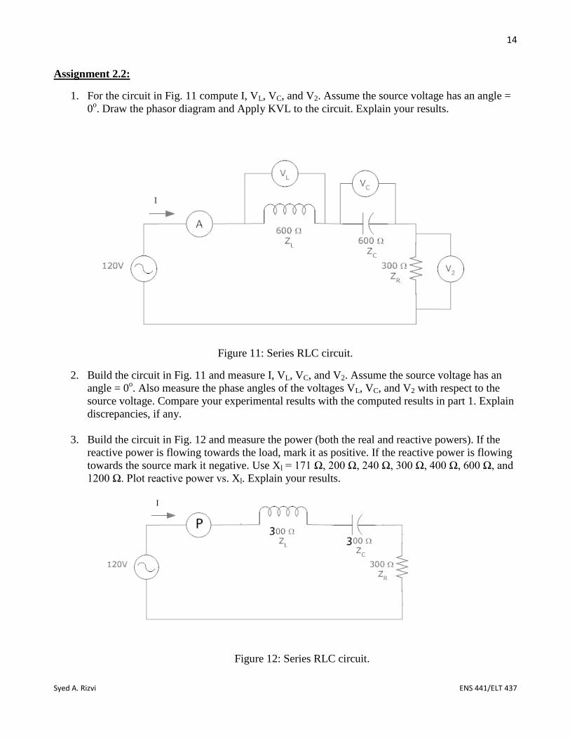
1. For the circuit in Fig. 11 compute I, VL, VC, and V2. Assume the source voltage has an angle =

0o. Draw the phasor diagram and Apply KVL to the circuit. Explain your results.


2. Build the circuit in Fig. 11 and measure I, VL, VC, and V2. Assume the source voltage has an

angle = 0o. Also measure the phase angles of the voltages VL, VC, and V2 with respect to the

source voltage. Compare your experimental results with the computed results in part 1. Explain

discrepancies, if any.

3. Build the circuit in Fig. 12 and measure the power (both the real and reactive powers). If the

reactive power is flowing towards the load, mark it as positive. If the reactive power is flowing

towards the source mark it negative. Use Xl = 171 Ω, 200 Ω, 240 Ω, 300 Ω, 400 Ω, 600 Ω, and

1200 Ω. Plot reactive power vs. Xl. Explain your results.


15


Per-Unit (pu) System of Measurements:

In per-unit system of measurements the quantities are expressed relative to a pre-defined reference

quantity. The reference quantity is called per-unit base of the system. A system can have a single per-

unit base quantity (such as voltage, current, power, impedance etc.). However, sometimes it is more

useful to have more than one base quantity (especially in electrical systems) such as voltage and power

as two per-unit base quantities. If we use power and voltage as the per-unit base quantities, we can

derive several other useful per-unit base quantities from them. Per-unit quantities are represented with

a subscript “B,” that is,

PB = per-unit base power

VB = per-unit base voltage.

If we know the per-unit base power (PB) and per-unit base voltage (VB) of the system we can find per-

unit current (IB) and per-unit impedance (ZB) of the system as follows

𝐼𝐵 =

𝑃𝐵

𝑉𝐵 (24)

and

𝑍𝐵 =

𝑉𝐵

𝐼𝐵. (25)

Example: A 10 Ω load (Rload) carries 25 A of current (Iload). If PB = 20 KW and VB = 400 V, calculate

per-unit voltage, current, power, and load resistance.

Solution: We will, first, calculate per-unit base current (IB) and impedance (ZB) as follows

𝐼𝐵 =𝑃𝐵

𝑉𝐵=

20000

400= 25 𝐴

and

𝑍𝐵 =𝑉𝐵

𝐼𝐵=

400

25= 8 Ω

We will now calculate load voltage (Vload) and power (Pload) as follows

𝑉𝑙𝑜𝑎𝑑 = 𝐼𝑙𝑜𝑎𝑑 × 𝑅𝑙𝑜𝑎𝑑 = 25 × 10 = 250 𝑉

and

𝑃𝑙𝑜𝑎𝑑 = 𝑉𝑙𝑜𝑎𝑑 × 𝐼𝑙𝑜𝑎𝑑 = 250 × 25 = 6250 𝑊

Finally, we can calculate p.u. quantities as follows

𝑝. 𝑢. 𝑃𝑜𝑤𝑒𝑟 =𝑃𝑙𝑜𝑎𝑑

𝑃𝐵=

6250

20000= 0.3125

16


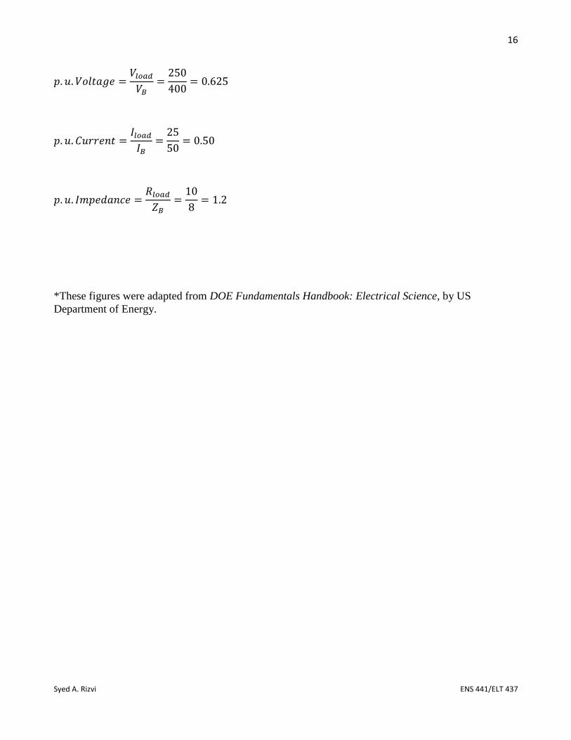
𝑝. 𝑢. 𝑉𝑜𝑙𝑡𝑎𝑔𝑒 =𝑉𝑙𝑜𝑎𝑑

𝑉𝐵=

250

400= 0.625

𝑝. 𝑢. 𝐶𝑢𝑟𝑟𝑒𝑛𝑡 =𝐼𝑙𝑜𝑎𝑑

𝐼𝐵=

25

50= 0.50

𝑝. 𝑢. 𝐼𝑚𝑝𝑒𝑑𝑎𝑛𝑐𝑒 =𝑅𝑙𝑜𝑎𝑑

𝑍𝐵=

10

8= 1.2

*These figures were adapted from DOE Fundamentals Handbook: Electrical Science, by US

Department of Energy.

17


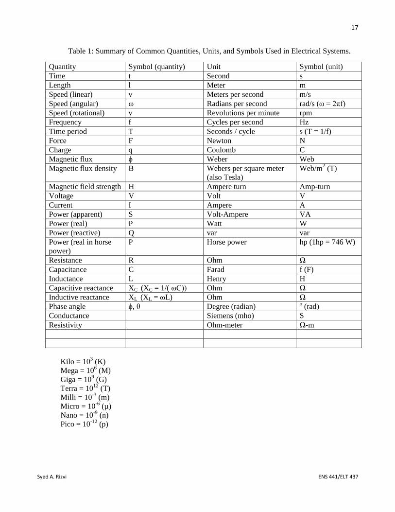
Table 1: Summary of Common Quantities, Units, and Symbols Used in Electrical Systems.

Quantity Symbol (quantity) Unit Symbol (unit)

Time t Second s

Length l Meter m

Speed (linear) v Meters per second m/s

Speed (angular) ω Radians per second rad/s (ω = 2πf)

Speed (rotational) v Revolutions per minute rpm

Frequency f Cycles per second Hz

Time period T Seconds / cycle s (T = 1/f)

Force F Newton N

Charge q Coulomb C

Magnetic flux ϕ Weber Web

Magnetic flux density B Webers per square meter

(also Tesla)

Web/m2 (T)

Magnetic field strength H Ampere turn Amp-turn

Voltage V Volt V

Current I Ampere A

Power (apparent) S Volt-Ampere VA

Power (real) P Watt W

Power (reactive) Q var var

Power (real in horse

power)

P Horse power hp (1hp = 746 W)

Resistance R Ohm Ω

Capacitance C Farad f (F)

Inductance L Henry H

Capacitive reactance XC (XC = 1/( ωC)) Ohm Ω

Inductive reactance XL (XL = ωL) Ohm Ω

Phase angle ϕ, θ Degree (radian) o (rad)

Conductance Siemens (mho) S

Resistivity Ohm-meter Ω-m

Kilo = 103 (K)

Mega = 106 (M)

Giga = 109 (G)

Terra = 1012

(T)

Milli = 10-3

(m)

Micro = 10-6

(µ)

Nano = 10-9

(n)

Pico = 10-12

(p)

1. ac fundamentals - city university of new york fundamentals.pdf · 1. ac fundamentals caution: in...

Documents