1

Analysis of Target Detection Performancefor Wireless Sensor Networks

Qing Cao, Ting Yan, John Stankovic, Tarek AbdelzaherDepartment of Computer Science, University of Virginia

Charlottesville Virginia 22904 USA{ qingcao, ty4k, stankovic, zaher }@cs.virginia.edu

Abstract

In surveillance and tracking applications, wireless sensor nodes collectively monitor the existence of intrudingtargets. In this paper, we derive closed form results for predicting surveillance performance attributes, representedby detection probability and average detection delay of intruding targets, based on tunable system parameters,represented by node density and sleep duty cycle. The results apply to both stationary and mobile targets, and shedlight on the fundamental connection between aspects of sensing quality and deployment choices. We demonstratethat our results are robust to realistic sensing models, which are proposed based on experimental measurements ofpassive infrared sensors. We also validate the correctness of our results through extensive simulations.

I. INTRODUCTION

A broad range of current sensor network applications involve surveillance. One common goal forsuch applications is reliable detection of targets with minimal energy consumption. Although maintainingfull sensing coverage guarantees immediate response to intruding targets, sometimes it is not favorabledue to its high energy consumption. Therefore, designers are willing to sacrifice surveillance quality inexchange for prolonged system lifetime. The challenge is to obtain the analytical relationship that depictsthe exact tradeoff between surveillance quality and system parameters in large-scale sensor networks. Inthis paper, we characterize surveillance quality by average detection delay and detection probability ofintruding targets. For system parameters, we are mainly concerned with duty cycle and node density. Thisknowledge answers the question of whether a system with a set of parameters is capable of achieving itssurveillance goals.

In this paper, we establish the relationship between system parameters and surveillance attributes.Our closed-form results apply to both stationary and moving targets, and are verified through extensivesimulations. Throughout this paper, we adopt the model of unsynchronized duty-cycle scheduling forindividual nodes. In this model, nodes sleep and wake-up periodically, which we call duty-cycling. Nodesagree on the length of the duty cycle period and the percentage of time they are awake within each dutycycle. However, the wakeup times are not synchronized among nodes. We call this model, random duty-cycle scheduling. There are two reasons for this choice. First, random scheduling is probably the easiest toimplement in sensor networks since it requires no coordination among nodes. Coordination among nodestakes additional energy and may be severely impaired by clock drifts. Second, many surveillance scenariospose the requirement of stealthiness (i.e. that nodes minimize their electronic signatures). Coordinatingnode schedules in an ad hoc network inevitably involves some message exchange which creates a detectableelectronic signature. In contrast, random scheduling does not require communication. Each node simplysets its own duty-cycle schedule according to the agreed-upon wakeup ratio, and starts surveillance. Noextra messages need to be exchanged before a potential target appears. Based on these two considerations,we focus this paper only on random duty-cycle scheduling.

We make two major contributions in this paper. First, for the first time, we obtain closed-form resultsto quantify the relationship between surveillance attributes and system parameters. The advantage is thatwe can now answer a variety of important questions without the need for simulation. For example, to

2

decrease the average detection delay for a potential target by half, how much should we increase thenode density? In this paper, we demonstrate that this problem, along with many others, can be answeredanalytically based on our results. Second, we propose a realistic (irregular) model of sensing based onempirical measurements. This model is then incorporated into our simulation to prove the robustnessof our analytic predictions. The results show that even under the irregular sensing model, the analyticclosed-form results are still quite accurate.

The rest of this paper is organized as follows. Section II presents the notations and assumptions ofthe paper. Section III considers stationary target detection. Section IV addresses mobile target detection.Section V presents the irregular sensing model based on experiments. Section VI discusses related workand Section VII concludes the paper.

II. NOTATIONS AND ASSUMPTIONS

In this section, we present the notations and assumptions for our derivations. First of all, we assumethat nodes are independently and identically distributed conforming to a uniform distribution. Density dis defined as the total number of nodes divided by area in which the system is deployed, Asystem. In ouranalysis, we adopt a simple sensing model in which a point is covered by a node if and only if the distancebetween them is less than or equal to the sensing range R of the node. For simplicity, we first assume thatall nodes have the same sensing range in all directions. We shall address sensing irregularity in SectionV. Each node is assumed to have a scheduling period T and a duty cycle ratio β, 0 ≤ β ≤ 1, that definesthe percentage of time the node is awake. Each node chooses its wakeup point tstart independently anduniformly within [0, T ), wakes up for a period of time βT , and then goes back to sleep until T + tstart.Finally, we assume that (for all practical purposes) the entire system area is covered when all nodes areawake.

Each target in the area moves in a straight line at a constant speed v in our analysis. We assume thatall targets are point targets so that their physical sizes can be neglected. Observe, however, that largertargets can still be analyzed by increasing the sensing range used in the analysis by the diameter of thetarget to account for the larger sensory signature.

III. STATIONARY TARGET SENSING ANALYSIS

In this section, we analyze the expected value and probability distribution of detection delay td for astationary, persistent target (e.g., a localized fire). We also derive the detection probability for a stationary,temporary event with a lifetime of T ′ (e.g., a conversation burst emanating from a fixed locale).

First, according to our assumptions, since nodes are deployed with a uniform distribution, the number ofnodes within an area of πR2 conforms to a binomial distribution B(Asystemd, πR2/Asystem). For a sensornetwork with a reasonable scale, Asystemd is a large number, and (Asystemd)(πR2/Asystem) = πR2d isa constant, denoted as λ. With these conditions, the binomial distribution can be approximated by aPoisson distribution with parameter λ. Observe that λ = πR2d is the average number of nodes withina sensing range. The probability that there are n nodes covering an arbitrary geometric point is λn

n!e−λ,

n = 0, 1, 2, .... The probability that no node covers the point (i.e., n = 0) is e−λ. To make this probabilitysmaller than 0.01, λ should be at least − ln 0.01 ≈ 4.6. Observe that the detection delay for points thatare not covered is infinite, which makes the expected detection delay for the whole area infinitely large.To avoid this problem, we take into account only those points that are covered by at least one node. Ourcalculations above indicate that as long as there are more than 4.6 nodes on average within a sensingrange, the probability that a point is not covered is less than 0.01, which is negligible.

In the rest of the paper, we extensively use two general results from theory of probability. First, ifthe probability of an event A occurring in a single experiment is p, and if the number of experimentsconforms to a Poisson Distribution with parameter λ, the probability of event A occurring at least oncein the series of experiments is:

P = 1 − e−pλ (1)

3

Node O

Start of Cycle T

Time Passage

Vigilant Period T

Fig. 1. Duty Cycle of a Particular Node O Fig. 2. Target Detection Scenarios

In the analysis, we first calculate the probability of detection when the target is covered by one nodein a certain area. Since the number of nodes in a certain area conforms to a Poisson distribution, we getthe probability that at least one node covers the target.

Another important result relating to our derivation is Proposition 11.6 in [16], which is stated as follows:Proposition 11.6: Let X be a nonnegative random variable, then

E(X) =

∫ ∞

0

P (X > x)dx (2)

Since the cumulative distribution function (CDF) of X cdf(x) = P (X ≤ x), we have

E(X) =

∫ ∞

0

(1 − cdf(x))dx (3)

We will use this fact to derive the average detection delay for both stationary and mobile target detection,after we get the probability that the target is detected within a certain period of time.

Now consider an arbitrary point in the area to be monitored. Suppose node O is the only node coveringthis point. The duty cycle of node O is shown in Figure 1. Denote the random variable corresponding tothe detection delay at this point as td. Since the node has a probability β of being awake, we have:

P (td = 0) = β (4)

The probability density function (PDF) of td f(τ), where 0 < τ ≤ T − βT , conforms to a uniformdistribution:

f(τ) =1

T(5)

as long as the target can arrive uniformly anywhere within the duty-cycle. Therefore, when there is onlyone node covering the point, the cumulative probability distribution for the detection delay is:

Ftd(τ) = P (td ≤ τ) = β +τ

T, (6)

where 0 ≤ τ ≤ T − βT . When there are n nodes covering the point, we consider the detection of eachnode as an experiment. Let event A correspond to the fact that the target is detected within an intervaltime no larger than td. Substituting for the single event probability p in Equation (1) from Equation (6)we get the probability of event A:

4

P (A) = 1 − e(−λτT

−βλ) (7)

Since we focus only on those points that are covered, the CDF of detection delay for such points isP (A)/1 − e−λ, or:

Ftd (τ) =1 − e(−λτ

T−βλ)

1 − e−λ, 0 ≤ τ ≤ T − βT (8)

where e−λ is the probability of voids.Second, according to Equation (3), the expected value of the delay td is:

E(td) =

∫ ∞

0P (td > t)dt =

∫ ∞

0

e−λ( tT

+β)

1 − e−λdt =

T

λe−βλ/(1 − e−λ) (9)

In particular, when the duty cycle β approaches 0 and 1− e−λ approaches 1, Equation (9) turns into T/λ.Therefore, we conclude that when the duty cycle is sufficiently small and the density is sufficiently large,the average detection delay is inversely proportional to node density.

Next, we extend the above result to temporary events with lifetime T ′. The key observation is thatthe detection probability for a temporary event with lifetime T ′ is the same as the probability that thedetection delay for a persistent target is less than or equal to T ′. Therefore, the detection probability is:

P (detection) =1 − e(−λT ′

T−βλ)

1 − e−λ(10)

This section derived the detection delay and detection probability for stationary targets under randomscheduling in large sensor networks with certain duty cycle and density. We shall validate these analyticresults through simulations. Next, we turn our attention to mobile targets.

IV. MOBILE TARGET SENSING ANALYSIS

In this section, we analyze the detection delay for mobile targets. We consider a target that moves atvelocity v along a straight path, and consider four detection scenarios, as shown in Figure 2. We categorizethese scenarios based on whether or not the start or end point of the target path is inside the system area.For target scenarios of type I and type IV (where the end-point is outside the monitored area), we areinterested in the probability that the target is detected by at least one node before it leaves the area. Fortarget scenarios of type II or type III (where the end-point is inside the monitored area), we are interestedin the expected time and distance the target travels before it is detected. The system area is assumed to berectangular, in which nodes are randomly deployed. The target is detected within a radius R (or diameter2R) which constitutes the width of the traversing areas shown in Figure 2. We focus on type I and typeII scenarios, and outline the results for the other two types.

We demonstrate a more detailed model for type II target detection in Figure 3 (type I model is similar).Consider the traversing area S consisting of the rectangle and two half-circles in the figure. For a potentialtarget that travels from point A to point B (where distance AB = L), only nodes located within this areacan detect the target, for example, node M , which has an intersection length of l with the target’s movingtrack. Therefore, we call this area the detection area. Since all nodes are deployed conforming to auniform distribution, the number of nodes in the detection area also conforms to Poisson Distributionapproximately. According to Equation (1) mentioned above, in order to find the probability of detection,we only need to find the detection probability when there is only one node within this area.

Now consider node M . Since it has an intersection length with the target track, the potential targettakes time l/v to pass its sensing area. Therefore, the target appears to be a temporary event with alifetime of l/v to node M , which means it has a probability of min(β + l

vT, 1) to be detected by node

M . Considering that node M could be anywhere within the detection area, we now analyze the averagedetection probability for node M to detect the target.

Notice that β+ lvT

can be at most 1,and if it is, the target will definitely be detected when it passes. Thisfact categorizes potential targets into two types, fast and slow. For fast targets, the expression β + l

vTis

5

L/2

R R

A B-L/2 ONode M

l

Fig. 3. Target Detection Example

L/2 R

L/2O

IntegralArea A

IntegralArea C

IntegralArea B

Fig. 4. Fast Target Detection

always smaller than or equal to 1. Therefore, we can obtain the expectation of detection delay directly byintegrating over the detection area. On the other hand, if v is small enough, β+ l

vTcan become larger than 1,

thus, we have to partition the detection area first before the integral. Observe that the maximal intersectionlength between the target path and a sensor’s range is 2R. Therefore, if target velocity v ≥ 2R

(1−β)T, then

β + lvT

is always smaller than or equal to 1. We use 2R(1−β)T

as the threshold between fast and slow targets.

A. Detection Analysis for Fast Targets

For a fast target we can express the probability that the target is detected given there is only one nodein the detection area, S, as follows:

P =

∫S(β +

l

vT)ds/S = β +

∫S lds

vTS(11)

Thus, we only need to calculate∫

Slds and S.

Because of symmetry, we only need to calculate the integral∫

Slds within the first quadrant, as shown

in Figure 4.For a type I target, we need to do the integral over area A and B, while for a type II target, we need

to do the integral over A, B and C.1) Fast Type I Target Analysis: For a type I target, the area under consideration consists of area A and

B. Therefore, we have: ∫SA+B

lds/SA+B =φA + φB

LR/2(12)

while

φA+B =

∫ R

0dy

∫ L2

02√

R2 − y2dx =πR2L

4(13)

Thus, we get the overall probability as:

P = β +πR2L

2RLvT= β +

πR

2vT(14)

2) Fast Type II Target Analysis: Similar to the type I target analysis, we have:∫

SA+B+C

lds/SA+B+C =φA + φB + φC

LR/2 + πR2/4(15)

Therefore,

φA =

∫ R

0dy

∫ L2 −

√R2−y2

02√

R2 − y2dx =πR2L

4− 4R3

3(16)

φB =

∫ R

0dy

∫ L2

L2 −

√R2−y2

(L

2+

√R2 − y2 − x)dx = R3 (17)

φC =

∫ R

0dy

∫ L2 +

√R2−y2

L2

(L

2+

√R2 − y2 − x)dx =

R3

3(18)

Thus, we get the overall probability as:

6

Node Q

B-L/2 O

Node M

l N

R

L/2-L/2-R L/2+RA

Fig. 5. Fast Target Detection Illustration

R

L

2aR

k(R,a)

Fig. 6. Slow Target Detection Illustration

P = β +πR2L

(2RL + πR2)vT= β +

πRL

(2L + πR)vT(19)

Note that for the case L < 2r, the derivation is a little different. However, the result remains the sameand for simplicity we omit the details of derivation.

We also have a more intuitive explanation for the calculation of∫

Slds. This expression is an integral

of a line segment of length l on the target’s locus for each point p in the traversing area S. Note that apoint p′ belongs to the line segment if and only if its distance from p is smaller or equal to R, the sensingrange. Therefore, the integral

∫S

lds is equivalent to the integral∫

Lsdl, where L is the locus of the target,

and s is the area in which each point has a shorter distance than R to dl. For type II targets, s is simplyπR2 and therefore

∫S

lds is simply πR2L, which verifies Equation (14). It is a little more complicated fortype I targets since s can be smaller than πR2. For example, for point N in Figure 5, s is a half-lens. Theexpression then becomes the integral of the overlapping area of the circular disk with radius R and thetraversing area over L. We can think it as a circular disk virtually moving from −L/2−R to L/2+R andcalculate the accumulation of overlapping areas. To make the calculation simpler, equivalently, we canalso imagine a fixed circular disk and virtually move the traversing area and calculate the accumulationoverlapping areas. This also gives a result of πR2L, which verifies Equation (19).

B. Detection Analysis for Slow Targets

Now consider v < 2R(1−β)T

. The main difference in this case is that it is possible that for certain nodepositions (x, y), l(x, y) > (1 − β)vT , therefore p(x, y) is 1 instead of β + l(x, y)/vT . Suppose there aretwo partitions, U and V . In U , p(x, y) = β + l(x, y)/vT , and in V , p(x, y) = 1. Therefore, we have:

P =

∫SU

(β + lvT

)ds +∫

SV1

SA+Bds =

∫SU+V

(β + lvT

)ds +∫

SV(1 − β − l

vT)ds

SU+V

= β +

∫SU+V

lds

(SU+V )vT+

SV (1 − β) − ∫SV

lds/vT

SU+V

Obviously, the term β +

∫SU+V

lds

(SA+B)vTis exactly what we have obtained for fast object analysis. So now we

need to calculate SV (1 − β) and∫

SVl. We classify the analysis into two cases according to type I and

type II targets.1) Slow Type I target Analysis: In this type, the partition where p(x, y) = 1 is the rectangle area A in

Figure 7. We define another variable a such that β +2a/vT = 1. The height of the rectangle is√

R2 − a2.

Observing thatSV (1−β)−∫

SVlds/vT

SU+V=

∫SV

[(1−β)vT−l(x,y)]dxdy

SU+V vT. Therefore, we have:

∫V

[(1 − β)vT − l(x, y)]dxdy =

∫A

[2a − l(x, y)]dxdy (20)

in which

7

L/2

2 2R a

)0,0(

A( / 2 ,0)L R

Fig. 7. Type I target Detection

L/22 2( / 2 , )L a R a

)0,0(

)0,22/( aLA B

( / 2 ,0)L R

Fig. 8. Regions A and B

∫∫A

[2a − l(x, y)]dxdy =

∫ √R2−a2

0

∫ L2

0(2a − 2

√R2 − y2)dxdy

=

∫ √R2−a2

0[aL − L

√R2 − y2]dy = aL

√R2 − a2 − L(

a√

R2 − a2

2+

R2

2sin−1

√R2 − a2

R)

= [aL√

R2 − a2 − LR2sin−1

√R2 − a2

R]/2

Therefore we obtain:

∫∫A

[2a − l(x, y)]dxdy = Lk(R, a)/4 (21)

wherek(R, a) = 2a

√R2 − a2 − 2R2cos−1(

a

R) (22)

Finally, we get when L ≥ 2R, v < 2R(1−β)T

, for a type I target,

P = β +πR2 + k(R, a)

2RvT(23)

2) Slow Type II target Analysis: In this type, the partition where p(x, y) = 1 is less regular. We stilldefine a such that β +2a/vT = 1. Observe Figure 8 plots the region where p(x, y) = 1, which includes Aand B, whose boundaries are formed by line y =

√r2 − a2 and two circles which centered at (L/2−2a, 0)

and (L/2, 0), respectively. For (x, y) ∈ A ∪ B, p(x, y) = 1.Similarly, we have: ∫

V[(1 − β)vT − l(x, y)]dxdy =

∫A+B

[2a − l(x, y)]dxdy (24)

in which

∫∫A

[2a − l(x, y)]dxdy =

∫ √R2−a2

0

∫ L2 −

√R2−y2

0(2a − 2

√R2 − y2)dxdy

=

∫ √R2−a2

0(L

2−

√R2 − y2)(2a − 2

√R2 − y2)dy

∫∫B

[2a − l(x, y)]dxdy =

∫ √R2−a2

0

∫ L2 −2a+

√R2−y2

L2 −

√R2−y2

[2a − (√

R2 − y2 − L

2− x)]dxdy

=

∫ √R2−a2

0[(2a −

√R2 − y2 − L

2)(2

√R2 − y2 − 2a) + 2a2 − aL − 2a

√R2 − y2 + L

√x2 − y2]dy

Therefore we can obtain:

∫∫A+B

[2a − l(x, y)]dxdy = (L − 2a)k(R, a)/4

8

wherek(R, a) = 2a

√R2 − a2 − 2R2cos−1(

a

R) (25)

Finally, we get when L ≥ 2R, v < 2R(1−β)T

, for a type II target,

P = β +πR2L + (L − 2a)k(R, a)

(2RL + πR2)vT(26)

Indeed, in Figure 8, we only plotted the case where 2a > R. For 2a < R, the derivation is similar, andthe results are the same.

When a = 0, k(R, a) = −πR2. When a = R, k(R, a) = 0. We also have

∂k(R, a)

∂a= 4

√R2 − a2 ≥ 0, (27)

so k(R, a) is a monotonically non-decreasing function of a. Interestingly, the area of B is exactly−k(R, a)/2.

Denote m(R, β) as the function substituting a with (1 − β)vT/2 in k(R, a), then

m(R, β) = (1 − β)vT

√R2 − (1 − β)2v2T 2

4− 2R2 cos−1[

(1 − β)vT

2R] (28)

m(R, β) is a monotonically non-increasing function of β. When β = 1− 2RvT

, m(R, β) = 0. When β = 1,m(R, β) = −πR2.

Additionally, for a slow type II target, if the travel distance L is less than (1 − β)vT , the detectionprobability for a node located within the detection area cannot be larger than 1. Therefore, we shouldtreat this period of time in the same way as a fast target. Therefore, we can revise the final probabilityas:

P = β +πR2L + min((L − 2a)k(R, a), 0)

(2RL + πR2)vT(29)

For slow targets, the intuitive understanding of the results is more complex. The absolute value of theadditional term k(R, a) corresponds to the overlapping area of two circular disks, as shown in Figure 6,which is the geometric representations of

∫S

lds and k(R, a).3) Average Detection Delay and Probability: So far, we have finished the derivation of P (L, v) for

both slow and fast objects. Next we go on to find the detection probability for a type I target, and averagedetection delay for a type II target.

First, consider fast targets. According to Equation 1, for a fast type I target, with a deployment widthof L, we obtain the detection probability as follows:

Pdetection(v) = 1 − e−2RLdP = 1 − e−2RLd(β+ πR2vT

) (30)

while for slow targets, the result is:

Pdetection(v) = 1 − e−2RLdP = 1 − e−2RLd(β+πR2+k(R,a)

2RvT)

For fast type II targets, the cumulative distribution function of the detection delay td is:

Ftd(t) = P (td ≤ t) = 1 − e−d(2Rvt+πR2)(β+ πRvt(2vt+πR)vT

) (31)

While for slow targets, the function is:

Ftd(t) = P (td ≤ t) = 1 − e−d(2Rvt+πR2)(β+

πR2vt+min(0,(vt−2a)k(R,a))

(2Rvt+πR2)vT)

9

For fast targets, the expected detection delay turns out to be

E(Td) =

∫ ∞

0

e−βπR2d−vt(2Rβ+πR2

vT)ddt =

e−βπR2d

(2Rβv + πR2

T)d

(32)

Similarly, when v < 2R(1−β)T

, the expected detection delay is1:

E(Td) =

∫ 2a

0e−βπR2d−vt(2Rβ+ πR2

vT)ddt +

∫ ∞

2ae−βπR2d+

2ak(R,a)dvT

−vt(2Rβ+πR2+k(R,a)

vT)ddt

=e−βπR2d

(2Rβv + πR2

T)d

[1 − m(R, β)e−(2RβvT+πR2)(1−β)d

2RβvT + πR2 + m(R, β)]

C. Summary

So far, we have finished the derivation for type I and type II targets, and we now briefly outline theresults for type III and type IV targets:

Expected detection delay for fast type III targets:

E(Td) =e−βπR2d/2

(2Rβv + πR2

T)d

(33)

Expected detection delay for slow type III targets:

E(Td) =e−βπR2d/2

(2Rβv + πR2

T)d

[1 − m(R, β)e−(2RβvT+πR2)(1−β)d

4RβvT + 2πR2 + m(R, β)]

Detection probability for fast type IV targets:

P = 1 − e−(2RL+πR2/2)d(β+ πRL(2L+πR/2)vT

) (34)

Detection probability for slow type IV targets:

P = 1 − e−(2RL+πR2/2)d(β+

πR2L+min((L−a)k(R,a),0)

(2RL+πR2/2)vT)

(35)

D. Discussion

We now discuss the implications of our analytical results. First, we assume that almost all of the areais covered, that is, 1−e−λ ≈ 1, thus, λ ≥ 4.6 according to our earlier discussion. Second, in order to saveenergy, we assume that β approaches 0, that is, the waking period is sufficiently small compared with thetotal scheduling period. Based on these two assumptions, we have several interesting observations.

First, for fast type I target detection, Equation (30) can be simplified to 1− e−λ

vTL. Therefore, in order

to obtain 99% detection probability, we have L ≥ 4.6vTλ

. Assume λ ≈ 4.6, L ≥ vT . The result is quiteintuitive: in order to almost certainly catch an intruding target, the deployment width can be no smallerthan the product of the target velocity and the scheduling period.

Second, for a fast type II target, Equation (31) can be simplified to 1 − e−λtT . This means that for a

target that starts from within the system area, the probability of being caught increases exponentially.Also, to make this probability larger than 99%, t ≈ T , given that λ is 4.6. This result is also confirmedin our simulations.

Third, for a type II target, the detection delay can be simplified as T/λ if β approaches 0. This resultis the same as the stationary detection delay, which means that as β approaches 0, regardless of themovement pattern of the target, the detection delay is approximately constant, determined only by thescheduling period and node density.

1Observe that if v = 0 (this is equivalent to a stationary target), we obtain the expected delay to be ∞. This is because we do not excludevoids in the mobile target model, and the existence of voids leads to infinitely large expected detection delay in stationary target detection.

10

0 0.1 0.2 0.3 0.4 0.5 0.6 0.7 0.8 0.9 1

0.4

0.5

0.6

0.7

0.8

0.9

1

1.1

Time (s)

cdf

Cumulative Distribution Function of Detection Delay (lambda=5)

Analytical - beta=0.1

Experimental - beta=0.1

Analytical - beta=0.2

Experimental - beta=0.2

Analytical - beta=0.3

Experimental - beta=0.3

Analytical - beta=0.4

Experimental - beta=0.4

Fig. 9. Stationary Detection Delay Distribution

0 0.1 0.2 0.3 0.4 0.5 0.6 0.7 0.8 0.9 10

0.02

0.04

0.06

0.08

0.1

0.12

0.14

0.16

0.18

0.2

duty cycle (beta)

Ave

rage

Det

ectio

n D

elay

(s)

Average Detection Delay for Static Target

Theoretical - lambda=5Theoretical - lambda=7Theoretical - lambda=9Thoeretical - lambda=11Experimental - lambda=5Experimental - lambda=7Experimental - lambda=9Experimental - lambda=11

Fig. 10. Average Stationary Detection Delay

E. Simulation Verification

We now demonstrate that the derivation results are consistent with simulation results under perfectcircular range assumptions. In the first set of simulations of stationary targets, locations of nodes aregenerated conforming to a uniform random distribution over a unit area with size 100m× 100m, withoutloss of generality. The period T is chosen to be 1s. The waking points of the nodes are generatedaccording to a uniform distribution over [0s, 1s]. The sensing range for circular model is 10m. We choosea point (50, 50) and generate 10, 000 sets of random target locations to run the simulations. The parameterλ = πr2d is set to 5. We record the the number of experiments where the detection delay is smallerthan or equal to 0s, 0.05s, 0.10s, ..., 0.90s, and 0.95s. We then compare these frequencies with thecumulative distribution functions (CDF’s) obtained in the analysis section. The simulation results areshown in Figure 9. From the figure we can see that our analysis and simulation results match well.

In the second set of simulations, we choose various λ values (5, 7, 9 and 11) and β values (0, 0.1,0.2, ..., 1), and run simulations to gather the average detection delays. Other settings are the same asthe previous set. We compare the average detection delays with the theoretical expected detection delaysobtained in the analysis section and plot Figure 10. The figure shows that the average delays are veryclose to the analytical expected delays.

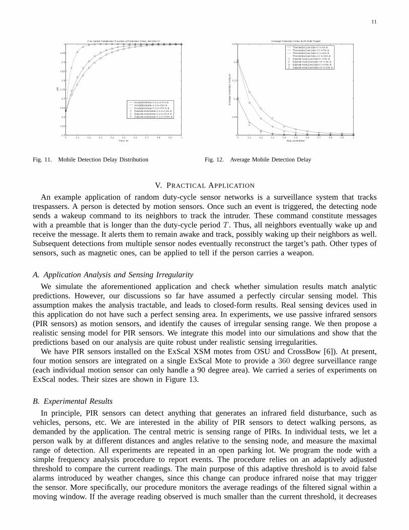
The settings for simulation verification with mobile target tracking are the same as the stationary setting,except that now the target has a velocity. We only consider type II target detection in this section, andother types can be similarly verified. The simulation result is shown in Figure 11. Observe that velocity2.5m/s means a slow target, according to our threshold. In particular, its cumulative detection probabilityhas a relatively long tail, compared to the distribution of targets with higher velocity, implying that forslower targets, there is a higher chance for the target to remain undetected after the scheduling cycle T .Again, we observe that our analysis and the simulation results match well.

In the second set of simulations, we choose various λ values (5 and 10), velocity (5m/s and 50m/s),and β values (0, 0.1, 0.2, ..., 1), and run simulations to gather the average detection delays. Other settingsare the same as in the previous set. We compare the average detection delays with the theoretical expecteddetection delays obtained in the analysis section and plot figure 12. The figure shows that the averagedelays are very close to the analytical expected delays.

The simulation results demonstrate the viability of using our results to predict the system performance.For example, suppose that we have a deployment of λ = 5 and T = 1s, in order to make sure that theexpected detection delay to be no larger than 0.1s, we can calculate that β must be at least 0.14. Thesimulation results confirm this calculation (Figure 10).

11

0 0.1 0.2 0.3 0.4 0.5 0.6 0.7 0.8 0.9 10.5

0.55

0.6

0.65

0.7

0.75

0.8

0.85

0.9

0.95

1Cum ulative Distribution Function of Detection Delay (lam bda=5)

Tim e (s)

cdf

Analytical-beta=0.2,v=2.5 m /sAnalytical-beta=0.2,v=25m /sAnalytical-beta=0.2,v=250 m /sExperim ental-beta=0.2,v=2.5m /sExperim ental-beta=0.2,v=25 m /sExperim ental-beta=0.2,v=250m /s

Fig. 11. Mobile Detection Delay Distribution

0 0.1 0.2 0.3 0.4 0.5 0.6 0.7 0.8 0.9 10

0.05

0.1

0.15

0.2

0.25

duty cycle(beta)

Average Detection Delay(s)

Average Detection Delay for M obile Target

Theoretical Lam bda=5 v=5m /sTheoretical Lam bda=10 v=5m /sTheoretical Lam bda=5 v=50m /sTheoretical Lam bda=10 v=50m /sExperim ental Lam bda=5 v=5m /sExperim ental Lam bda=10 v=5m /sExperim ental Lam bda=5 v=50m /sExperim ental Lam bda=10 v=50m /s

Fig. 12. Average Mobile Detection Delay

V. PRACTICAL APPLICATION

An example application of random duty-cycle sensor networks is a surveillance system that trackstrespassers. A person is detected by motion sensors. Once such an event is triggered, the detecting nodesends a wakeup command to its neighbors to track the intruder. These command constitute messageswith a preamble that is longer than the duty-cycle period T . Thus, all neighbors eventually wake up andreceive the message. It alerts them to remain awake and track, possibly waking up their neighbors as well.Subsequent detections from multiple sensor nodes eventually reconstruct the target’s path. Other types ofsensors, such as magnetic ones, can be applied to tell if the person carries a weapon.

A. Application Analysis and Sensing Irregularity

We simulate the aforementioned application and check whether simulation results match analyticpredictions. However, our discussions so far have assumed a perfectly circular sensing model. Thisassumption makes the analysis tractable, and leads to closed-form results. Real sensing devices used inthis application do not have such a perfect sensing area. In experiments, we use passive infrared sensors(PIR sensors) as motion sensors, and identify the causes of irregular sensing range. We then propose arealistic sensing model for PIR sensors. We integrate this model into our simulations and show that thepredictions based on our analysis are quite robust under realistic sensing irregularities.

We have PIR sensors installed on the ExScal XSM motes from OSU and CrossBow [6]). At present,four motion sensors are integrated on a single ExScal Mote to provide a 360 degree surveillance range(each individual motion sensor can only handle a 90 degree area). We carried a series of experiments onExScal nodes. Their sizes are shown in Figure 13.

B. Experimental Results

In principle, PIR sensors can detect anything that generates an infrared field disturbance, such asvehicles, persons, etc. We are interested in the ability of PIR sensors to detect walking persons, asdemanded by the application. The central metric is sensing range of PIRs. In individual tests, we let aperson walk by at different distances and angles relative to the sensing node, and measure the maximalrange of detection. All experiments are repeated in an open parking lot. We program the node with asimple frequency analysis procedure to report events. The procedure relies on an adaptively adjustedthreshold to compare the current readings. The main purpose of this adaptive threshold is to avoid falsealarms introduced by weather changes, since this change can produce infrared noise that may triggerthe sensor. More specifically, our procedure monitors the average readings of the filtered signal within amoving window. If the average reading observed is much smaller than the current threshold, it decreases

12

Fig. 13. Illustration of ExScal Sensor Node

20

40

60

80

100

120

140

160

180

200

220

240

260

280

300

0 30 60 90 120 150 180 210 240 270 300 330 360

Sen

sing

Ran

ge(in

ches

)

Direction(degrees)

Node ANode B

Fig. 14. Sensing Range with Different Directions

the threshold by taking a weighted average. On the other hand, if the average energy is close to or largerthan the threshold for a certain period, the sensor decides that the weather is noisy, and increases thethreshold. Practically we are able to filter out almost all false alarms using this technique. We note thatthis technique also filters out those slight disturbances that may, in fact, be caused by the target. Thus, theresults proposed below present effective sensing range in slightly noisy environments, which are differentfrom precisely controlled environments.

We measured the sensing range from 24 equally divided directions. At each direction, a person moveswith different distances from the sensor node. If the fluctuation of the filtered sensor reading exceeds apredefined noise threshold due to the nearby motion, the measured point is within the sensing range. Ifthe motion does not cause a fluctuation greater than the threshold, the measured point is out of the sensingrange. In the experiments we found out that the sensitivity of the sensors changes dramatically at the edgeof the sensing range. The motion can always be detected in the sensing range and the motion 10 inchesbeyond the sensing range never triggers the sensors. Therefore, the precision of the range measurementis always within 10 inches (the range itself being hundreds of inches). The experimental results for tworepresentative nodes are shown in Figure 14. Obviously, with four sensors, the range is far from beingcircular. A more intuitive illustration is shown in Figure 15, where the sensing range in each direction isplotted to scale.

Based on the experimental results of multiple tests, we have the following observations regarding the PIRsensing capability. First, the sensing range of one node is not isotropic, that is, the node exhibits differentranges in different directions. Second, the boundary of the sensing range is delineated quite sharply, withpredictably no detection when the range is exceeded by about 3-7%. Third, we can consider the variationof ranges relatively continuous. We do observe sudden changes in the sensitivity of some nodes, but thisis very uncommon. Therefore, a model may consider connecting sensitivity ranges in different directionsusing continuous curves. Forth, the sensing range distribution in different directions roughly conforms toa Normal Distribution. This conclusion is based on statistical analysis of our experimental data using aKolmogorov-Smirnov Test [26]. We concluded from our experimental data set that the sensing range inone direction can be approximated with a Normal Distribution with an expectation of 217 inches and astandard deviation of 32 inches.

C. Realistic Sensing Model for PIR sensors

In this section, we present a realistic sensing model for PIR nodes. This model is designed to reflectthe three key observations: non-isotropic range, continuity and normality. First, the model determinessensing ranges for a set of equally-spaced directions. Each range can either be specified based onactual measurements or obtained from a representative distribution, for example, the normal distributionN(217, 322). Next, sensing ranges in all other possible directions are determined based on a interpolationmethod. For simplicity, we use linear interpolation to specify the boundary of the sensing area. As an

13

Fig. 15. Sensing Range of Two Nodes Fig. 16. Approximations of Realistic Range

0 0.1 0.2 0.3 0.4 0.5 0.6 0.7 0.8 0.9 10.3

0.4

0.5

0.6

0.7

0.8

0.9

1

1.1

Time(s)

cdf

Analytical−beta=0.1Analytical−beta=0.2Analytical−beta=0.3Analytical−beta=0.4Realistic Experimental−beta=0.1Realistic Experimental−beta=0.2Realistic Experimental−beta=0.3Realistic Experimental−beta=0.4

Cumulative Distribution for Stationary Target Detection Delay under Realistic Sensing Model

Fig. 17. Realistic Sensing Effect

0 0.1 0.2 0.3 0.4 0.5 0.6 0.7 0.8 0.9 10.6

0.65

0.7

0.75

0.8

0.85

0.9

0.95

1

Time(s)

cdf

Analytical−beta=0.2,v=2.5 m/sAnalytical−beta=0.2,v=25 m/sAnalytical−beta=0.2,v=250 m/sRealistic Experimental−beta=0.2,v=2.5 m/sRealistic Experimental−beta=0.2,v=25 m/sRealistic Experimental−beta=0.2,v=250 m/s

Cumulative Distribution Function of Detection Delay under Realistic Sensing Model (lambda = 5)

Fig. 18. Realistic Sensing Effect

0.00%

0.20%

0.40%

0.60%

0.80%

1.00%

1.20%

0 0.05 0.1 0.15 0.2 0.25 0.3 0.35 0.4 0.45 0.5 0.55 0.6 0.65 0.7 0.75 0.8 0.85 0.9 0.95 1

Time(s)

Err

or

rela

tive

to

Pre

dic

tio

n V

alu

e

Stationary beta=0.2 Realistic Range Model

Stationary beta=0.4 Realistic Range Model

Mobile beta=0.2 v=2.5m/s Realistic Range Model

Mobile beta=0.2 v=25m/s Realistic Range Model

Mobile beta=0.2 v=250m/s Realistic Range Model

Fig. 19. Robustness of Theoretical Predictions

example, the approximation of the two representative nodes based on this model are shown in Figure 16.Clearly, our simplified model pretty accurately reflects the fluctuations of sensing ranges in differentdirections.

D. Additional Notes

Despite the fact that we proposed a realistic sensing model based on experimental results for PIRsensor, we have simplified many other aspects of the application. For the detection part, we assumed thatindividual node duty cycle is so large that the sensor warmup time is negligible. We also assumed that theexistence of targets within sensing range can be determined in sufficiently short time. For the target part,we also do not address more complex movements of the target. We acknowledge that introduction of anyof these factors will considerably increase the complexity of the analysis. However, our analysis is stillinnovative and useful in the sense that it reveals quantitative relationships between system parameters andperformance. Such understanding will considerably advance our knowledge of the underlying principlesof the design and deployment of general sensor networks.

E. Robustness of Theoretical Predictions to Realistic Sensing Model

We now incorporate the realistic sensing range model into simulations to test the robustness of the perfor-mance predictions to sensing irregularity. We scaled the normal distributionN(217, 322) to N(10, 1.472)to fit the simulation setting. To illustrate the difference, we also plot the error relative to theoreticalpredictions. The results are shown in Figure 17 to Figure 19.

We have two observations regarding these results. First, sensing irregularity has a very small effect.One primary reason is that even though the detection ranges do vary with different directions, the overalldegree of coverage for the area remains almost the same, approximated byλ. Therefore, the overall

14

detection delay distribution is almost not affected. Second, we observe that the maximal error relative totheoretical predictions is no more than 1.2%. As an example to show its implications, suppose that wehave a set of system parameters that guarantees that 99% of intruding targets are detected within a certaintime. Then, the actual detection rate should be no less than 97% with the existence of irregularity. Basedon this observation, we conclude that our model is quite robust to realistic sensing conditions.

At last, we acknowledge that so far, our modeling of the realistic sensing model is only concernedwith PIR sensors. Other types of sensors may well exhibit different characteristics, therefore, may havevaried effect on the detection performance. However, we envision that with a relatively large systemwith considerable density, the effect of sensing irregularity will be considerably limited, leading toimprovements in the accuracy of the aforementioned results.

VI. RELATED WORK

Research on minimizing energy consumption has been one central topic in the sensor network com-munity in recent years. Various effective techniques have been proposed, evaluated and implemented.Protocols to schedule nodes while maintaining full coverage have been proposed by [25], [29], [22], [10].The full sensing coverage model is very suitable for areas where continuous vigilance is required, butconsumes considerable energy. There exists a lower bound on the minimal energy consumption if therequirement of full sensing coverage is to be fulfilled. To guarantee a longer sensor network lifetime, incertain situations, the designer may wish to keep partial sensing coverage in exchange of longer productlifetime.

Recent research efforts [9], [17], [11] has turned attention to the study of target tracking in the contextof partial sensing coverage. In [9], the authors proposed the metric of quality of surveillance, which isdefined as the average traveled distance of the target before it is detected. This is consistent with themodel in our paper, where the average detection delay rather than distance is used. However, the authorsdidn’t address the precise determination of this metric, instead, they used an approximation model basedon coverage process theory. Their attention is mainly focused on evaluating various sleep models inrespect to the average travel length, which lead to considerably different results compared with ours. Thework in [17] considers an equivalent problem to the type II target detection of our paper. However, we aremore interested in deriving closed-form expressions for all four scenarios, whereas [17] only considers fasttargets and does not present closed-form results for detection delay or stealth distance. Another interestingwork is [11], which considered the effect of different random and coordinated scheduling approaches.However, none of these papers derived the closed form results as in our paper, and therefore, we believeour work is a necessary complement towards thorough understanding of detection delay performance.

VII. CONCLUSION

This paper is the first to derive closed-form formulas for the distribution and expectation of detectiondelay for both stationary and mobile targets, and is also the first to propose and evaluate a realistic sensingmodel for sensor networks, to the best of the authors’ knowledge. Extensive simulations are conducted andthe results show the validity of the analysis. The analytical results are of high importance for designersof energy efficient sensor networks for monitoring and tracking applications. Designers can apply theseformulas to predict the detection performance without costly deployment and testing. Based on theseformulas, they can make decisions on key system or protocol parameters, such as the network densityand the duty cycle, according to the detection requirements of the system. Therefore, this work is a majorcontribution towards a thorough understanding of the relationship between system and protocol parametersand achievable detection performance metrics.

REFERENCES

[1] J. Aslam, Z. Butler, F. Constantin, V. Crespi, G. Cybenko, and D. Rus. Tracking a moving object with a binary sensor network. InProceedings of Sensys, 2003.

15

[2] M. Batalin, M. Rahimi, Y. Yu, S. Liu, G. Sukhatme, and W. Kaiser. Call and response: Experiments in sampling the environment. InProceedings of Sensys, 2004.

[3] K. Chakrabarty, S. S. Iyengar, H. Qi, and E. Cho. Grid coverage for surveillance and target location in distributed sensor networks. InIEEE Transaction on Computers, 51(12), 2002.

[4] B. J. Chen, K. Jamieson, H. Balakrishnan, and R. Morris. Span: An energy-efficient coordination algorithm for topology maintenancein ad hoc wireless networks. In Proceedings of Mobicom, 2002.

[5] C. F. Chiasserini and M. Garetto. Modeling the performance of wireless sensor networks. In IEEE Infocom, 2004.[6] CrossBow. In http://www.xbow.com.[7] D. Ganesan, R. Cristescu, and B. Berefull-Lozane. Power-efficient sensor placement and transmission structure for data gathering under

distortion constraints. In Proceedings of IPSN, 2004.[8] D. Goldberg, A. Andreou, P. Julian, P. Pouliquen, L. Riddle, and R. Rosasco. A wake-up detector for an acoustic surveillance sensor

network: Algorithm and vlsi implementation. In Information Processing in Sensor Networks (IPSN), 2004.[9] C. Gui and P. Mohapatra. Power conservation and quality of surveillance in target tracking sensor networks. In ACM Mobicom, 2004.

[10] T. He, S. Krishnamurthy, J. Stankovic, T. Abdelzaher, L. Luo, R. Stoleru, T. Yan, L. Gu, J. Hui, and B. Krogh. An energy-efficientsurveillance system using wireless sensor networks. In the Second International Conference on Mobile Systems, Applications andServices (MobiSys), 2004.

[11] C. Hsin and M. Y. Liu. Network coverage using low duty-cycled sensors: Random and coordinated sleep algorithms. In InformationProcessing in Sensor Networks(IPSN), 2004.

[12] J. J. Liu, J. Liu, J. Reich, P. Cheung, and F. Zhao. Distributed group management for track initiation and maintenance in targetlocalization applications. In Proceedings of IPSN, 2003.

[13] S. Megerian, F. Koushanfar, G. Qu, and M. Potkonjak. Exposure in wireless sensor networks. In Proceedings of Mobicom, 2001.[14] S. Meguerdichian, F. Koushanfar, M. Potkonjak, and M. B. Srivastava. Coverage problems in wireless ad-hoc sensor networks. In

Proceedings of IEEE Infocom, 2001.[15] S. Pattem, S. Poduri, and B. Krishnamachari. Energy-quality tradeoff for target tracking in wireless sensor networks. In Proceedings

of IPSN, 2003.[16] S. Port. Theoretical Probability for Applications. John Wiley and Sons,Inc, 1994.[17] S. Ren, Q. Li, H. N. Wang, X. Chen, and X. D. Zhang. Probabilistic coverage for object tracking in sensor network. In Mobicom

2004 Poster Session, 2004.[18] C. Schurgers, V. Tsiatsis, S. Ganeriwal, and M. Srivastava. Optimizing sensor networks in the energy-latency-density design space. In

IEEE Transactions on Mobile Computing, 2002.[19] V. Shnayder, M. Hempstead, B. R. Chen, G. W. Allen, and M. Welsh. Simulating the power consumption of large-scale sensor network

applications. In the Second ACM Conference on Embedded Networked Sensor Systems (SenSys), 2004.[20] G. Simon, A. Ledeczi, and M. Maroti. Sensor network-based countersniper system. In Proceedings of Sensys, 2004.[21] R. Szewczyk, A. Mainwaring, J. Polastre, and D. Culler. An analysis of a large scale habitat monitoring application. In Proceedings

of Sensys, 2004.[22] D. Tian and N. D. Georganas. A node scheduling scheme for energy conservation in large wireless sensor networks. In Wireless

Communications and Mobile Computing Journal, 2003.[23] G. Veltri, Q. F. Huang, G. Qu, and M. Potknonjak. Minimal and maximal exposure path algorithms for wireless embedded sensor

networks. In Proceedings of Sensys, 2003.[24] P. J. Wan, K. M. Alzoubi, and O. Frieder. Distributed construction of connected dominating set in wireless ad hoc networks. In IEEE

Infocom, 2002.[25] X. R. Wang, G. L. Xing, Y. F. Zhang, C. Y. Lu, R. Pless, and C. Gill. Integrated coverage and connectivity configuration in wireless

sensor networks. In First ACM Conference on Embedded Networked Sensor Systems (SenSys), 2003.[26] E. W. Weisstein. Kolmogorov-smirnov test. In MathWorld at http://mathworld.wolfram.com/Kolmogorov-SmirnovTest.html.[27] J. Wu and M. Gao. On calculating power-aware connected dominating sets for efficient routing in ad hoc wireless networks. In

Proceedings of the 30th Annual International Conference On Parallel Processing, 200l.[28] N. Xu, S. Rangwala, K. Chintalapudi, D. Ganesan, A. Broad, R. Govindan, and D. Estrin. A wireless sensor network for structural

monitoring. In Proceedings of SenSys 2004, 2004.[29] T. Yan, T. He, and J. A. Stankovic. Differentiated surveillance for sensor networks. In First ACM Conference on Embedded Networked

Sensor Systems (SenSys), 2003.[30] F. Ye, G. Zhong, J. Cheng, S. W. Lu, and L. X. Zhang. Peas:a robust energy conserving protocol for long-lived sensor networks. In

IEEE International Conference on Distributed Computing Systems(ICDCS), 2003.