J.Stat.M

ech.(2006)

P06018

ournal of Statistical Mechanics:An IOP and SISSA journalJ Theory and Experiment

Exact asymptotic expansions for thecylindrical Poisson–Boltzmann equation

Gabriel Tellez1 and Emmanuel Trizac2,3

1 Departamento de Fısica, Universidad de Los Andes, AA 4976, Bogota,Colombia2 CNRS, Universite Paris Sud, UMR 8626, LPTMS, Orsay Cedex, F-91405,France3 Center for Theoretical Biological Physics, UC San Diego, 9500 Gilman DriveMC 0374, La Jolla, CA 92093-0374, USAE-mail: gtellez@uniandes.edu.co and trizac@lptms.u-psud.fr

Received 24 February 2006Accepted 2 June 2006Published 28 June 2006

Online at stacks.iop.org/JSTAT/2006/P06018doi:10.1088/1742-5468/2006/06/P06018

Abstract. The mathematical theory of integrable Painleve/Toda type systemssheds new light on the behaviour of solutions to the Poisson–Boltzmann equationfor the potential due to a long rod-like macroion. We investigate here the caseof symmetric electrolytes together with that of 1:2 and 2:1 salts. Small andlarge scale features are analysed, with particular emphasis on the low salinityregime. Analytical expansions are derived for several quantities relevant forpolyelectrolyte theory, such as the Manning radius. In addition, accurate andpractical expressions are worked out for the electrostatic potential, which improveupon previous work and cover the full range of radial distances.

Keywords: complex fluids, polymers

c©2006 IOP Publishing Ltd and SISSA 1742-5468/06/P06018+31$30.00

J.Stat.M

ech.(2006)

P06018

Exact asymptotic expansions for the cylindrical Poisson–Boltzmann equation

Contents

1. Introduction 2

2. Formal solution to the problem 4

3. Asymptotic expansions 63.1. Short distance behaviour . . . . . . . . . . . . . . . . . . . . . . . . . . . . 63.2. Connecting small and large scale features . . . . . . . . . . . . . . . . . . . 83.3. Applying the boundary condition at polyion contact . . . . . . . . . . . . . 93.4. What are the associated threshold potentials and charges? . . . . . . . . . 10

4. A few limiting cases 124.1. a = 0 and arbitrary ξ . . . . . . . . . . . . . . . . . . . . . . . . . . . . . . 124.2. ξ → 0 and arbitrary a < 1 . . . . . . . . . . . . . . . . . . . . . . . . . . . 154.3. ξ = ξManning and arbitrary a < 1 . . . . . . . . . . . . . . . . . . . . . . . . 164.4. ξ > ξManning and arbitrary a < 1 . . . . . . . . . . . . . . . . . . . . . . . . 16

5. Results at finite salt and discussion 175.1. Counterion condensation and Manning radius . . . . . . . . . . . . . . . . 175.2. Effective charges . . . . . . . . . . . . . . . . . . . . . . . . . . . . . . . . 225.3. Electric potential . . . . . . . . . . . . . . . . . . . . . . . . . . . . . . . . 23

6. Effective charge at saturation and the largest eigenvalue of the operators Ka 23

7. Conclusion 26

Acknowledgments 28

Appendix A: Painleve classification; a brief reminder 28

Appendix B: Short distance behaviour for λ > λc 29

References 31

1. Introduction

Polyelectrolytes are polymer molecules bearing charged units. Within the associatedrelevant cylindrical geometry, the long range character of Coulombic interactions isresponsible for the phenomenon of counterion condensation. In essence, the electricpotential created by the charged polyion features a logarithmic dependence on radialdistance. The competing entropy of confinement is of a similar functional form,which may result in a condensation of counterions onto the charged cylinder, whenCoulombic interactions prevail, that is when the polyelectrolyte line charge exceeds agiven threshold (see e.g. [1]). Strongly charged linear polyelectrolytes thereby effectivelyreduce their line charge density. This was realized by Onsager in the 1960s and formalizedsubsequently [2, 3]. It turns out that the mean field Poisson–Boltzmann (PB) theory

doi:10.1088/1742-5468/2006/06/P06018 2

J.Stat.M

ech.(2006)

P06018

Exact asymptotic expansions for the cylindrical Poisson–Boltzmann equation

offers a valuable framework for discussing and analysing the phenomenon in detail [4]–[15]. Unfortunately, even within the mean field, exact results are scarce, and one has toresort to numerical resolution or propose approximations.

This paper is dedicated to the derivation of exact results within PB theory. We willbe interested in the behaviour of a unique infinite charged cylinder of radius a and uniformline charge density e/b, where e > 0 is the elementary charge and b may be viewed as anequivalent average spacing between charges along the polyion. This macroion is immersedin an infinite electrolyte containing two species of microions (salt): their bulk densities n1

and n2 far from the cylinder define the Debye length 1/κ through κ2 = 4πB(n1z21 +n2z

22).

Here, zie denotes the charge of species i and B = βe2/ε is the Bjerrum length, whichinvolves the solvent dielectric permittivity ε and the inverse temperature β. We will focuson the three situations where analytical progress is possible: 1:1 electrolytes (or moregenerally symmetric z:z electrolytes), together with the 1:2 and 2:1 cases. We denote by1:2 the situation where coions are monovalent (z+ = 1 for a positively charged polyion) andcounterions are divalent (z− = −2 or more generally, z− = −2z+). On the other hand,the notation 2:1 refers to divalent coions with monovalent counterions. To be specific,introducing the dimensionless radial distance r = κr, the equations to be solved for thedimensionless electrostatic potential y = βeψ (ψ being the electric potential) read

d2y

dr2+

1

r

dy

dr= sinh(y) (1:1) (1.1a)

d2y

dr2+

1

r

dy

dr=

1

3

(e2y − e−y

)(1:2) (1.1b)

d2y

dr2+

1

r

dy

dr=

1

3

(ey − e−2y

)(2:1). (1.1c)

The solution should satisfy the boundary conditions at a = κa

limr→a

rdy

dr= −2 ξ (1.2)

and limr→∞ y(r) = 0. We have introduced here the dimensionless bare line chargeξ = B/b, that plays a key role below. It is understood that the cylinder is positivelycharged, without loss of generality4.

We shall not comment here the well documented limitations of the mean fieldapproximation (see e.g. [16]–[21]), but only summarize the main findings. In a solventlike water at room temperature, mean field provides an accurate description in the 1:1case for all existing polyelectrolytes. We also expect the 2:1 situation to be correctlydescribed, while in the 1:2 case, microionic correlations, discarded within the meanfield, play an important role at large values of ξ. Schematically, the coupling parameterΓ = z3/2

√ξB/(2πa) allows one to appreciate the importance of those correlations where

z stands for the counterion valency. When Γ < 2, the mean field holds.The crux of our approach lies in the mapping between equations (1.1) and

Painleve/Toda type equations (see below), that are in particular relevant for describing thespin–spin correlator in the two-dimensional Ising model, and have been the subject of deep

4 Note that the 1:2 case with ξ > 0, with coions of valency z1 = +1 and counterions of valency z2 = −2, isidentical to the case z1 = +2, z2 = −1 with ξ < 0. Equation (1.1c) and the boundary condition (1.2) is of courseformally equivalent to equation (1.1b) after the substitutions y → −y and ξ → −ξ.

doi:10.1088/1742-5468/2006/06/P06018 3

J.Stat.M

ech.(2006)

P06018

Exact asymptotic expansions for the cylindrical Poisson–Boltzmann equation

mathematical investigations [22]–[24]. It seems that this body of work has not been fullytransposed into the language of polyelectrolyte physics, with the exception of for the limitκa → 0+ (e.g. realized with a charged line—of vanishing thickness—at finite salt) whereit allowed several authors to show rigorously the existence of the condensation [9, 10] andalso provided exact results for the electric potential [9, 11]. However, it will appear belowthat the limit κa → 0+ is approached logarithmically slowly so that finite salt correctioncannot be neglected in practice. It also turns that to the best of our knowledge, thecase of 2:1 electrolytes has not been considered in the physics literature, whereas someresults have been reported in the reverse 1:2 case, but below the condensation thresholdand again in the limit a → 0 [11]. Our aim is to fill these gaps. Our formulae will proveextremely accurate when compared to the numerical solutions of (1.1).

The paper is organized as follows. In section 2, the formal solutions of equations (1.1)will be given. As such, these relations are not useful in practice, and deriving ‘ready-to-use’ and operational expressions will be the purpose of the subsequent analysis. Section 3will then be devoted to the derivation of asymptotic expansions for the electric potential,and to the connection between short and long distance features. These results identifya change in the short distance behaviour when increasing the charge density above athreshold ξc, which will be worked out. This is the fingerprint of counterion condensation,which turns out to be smoothed by salt (strictly speaking, the phenomenon is critical inthe limit κa → 0 only). Section 4 will analyse a few limiting cases of particular interest.Analytical expressions for several important quantities such as the Manning radius willbe given and compared in section 5 to the numerical data obtained solving the non-linearPB equation. A similar analysis will be performed for the electric potential, which willassess the validity of the analytical results. Although particular attention will be paid tothe low salinity regime (the results of sections 3–5 rely on expansions that typically breakdown for κa > 1), we will also report in section 6 some results concerning the effectivecharge of the polyion, valid for all values of κa. A preliminary account of parts of thiswork has been published in [25].

Before embarking on the analysis of the properties of equations (1.1), we note that fora macroion with a small reduced linear charge density ξeff , the problem may be linearizedwith the solution

ylin(r) =2ξeff

aK1(a)K0(r). (1.3)

Here K0 and K1 are the modified Bessel functions. Since the solution to the non-linearproblem (1.1) vanishes when r → ∞ we necessarily have that for large distances r, y(r)behaves as (1.3). However in the non-linear case the constant ξeff is not the bare chargeof the rod. This quantity is called the effective charge and depends on salinity conditions,bare charge, temperature etc. In the weak overlap approximation where the double layersof different macroions are well separated (it is typically the case when their mutual distanceis larger than 1/κ), the (squared) effective charge governs the amplitude of the interactionfree energy.

2. Formal solution to the problem

The Poisson–Boltzmann equation (1.1a) in the 1:1 case has been solved in [22] in thecontext of the Painleve III theory, since ey/2 obeys a particular case of the Painleve III

doi:10.1088/1742-5468/2006/06/P06018 4

J.Stat.M

ech.(2006)

P06018

Exact asymptotic expansions for the cylindrical Poisson–Boltzmann equation

equation (see e.g. [26] and appendix A; more details together with a relevant bibliographymay be found in [27]). More generally, equations (1.1a), (1.1b) and (1.1c) are the firstequations of the hierarchy of cylindrical Toda equations. In [23], a class of solutionsto these Toda equations has been reported, and hence the solutions to the Poisson–Boltzmann equations (1.1a), (1.1b) and (1.1c). These solutions obey a boundary conditionat r → ∞, given in terms of a constant λ by

y11(r) ∼ 4λK0(r) (2.1a)

for the 1:1 case,

y(r) ∼ 6λK0(r) (2.1b)

for both 1:2 and 2:1 cases.The solutions are expressed as determinants of certain operators. For 1:1 salts, we

have

y11(r) = 2 ln det(1 + λKr) − 2 ln det(1 − λKr) (2.2)

with Kr an integral operator on R+ with kernel

Kr(u, v) =exp(−r(u + u−1)/2)

u + v. (2.3)

In the 1:2 case the solution reads

y12(r) = ln det(1 − λK(0)r ) − ln det(1 − λK

(2)r ) (2.4)

while in the 2:1 situation it is

y21(r) = ln det(1 + λK(2)r ) − ln det(1 + λK

(1)r ) (2.5)

where

K(0)r = (ζ − ζ2)O

(1)r + (ζ2 − ζ)O

(2)r (2.6a)

K(1)r = (ζ2 − 1)O

(1)r + (ζ − 1)O

(2)r (2.6b)

K(2)r = (1 − ζ)O

(1)r + (1 − ζ2)O

(2)r . (2.6c)

Here ζ = ei2π/3 and O(1)r and O

(2)r are integral operators on R

+ with kernel

O(1)r (u, v) =

exp(−r[(1 − ζ)u + (1 − ζ2)u−1]/(2√

3))

−ζu + v(2.7)

and O(2)r (u, v) = O

(1)r (u, v), the bar denoting complex conjugation. It can be shown [23]

that det(1 − λK(1)r ) = det(1 − λK

(0)r ) (making use of a change of variable u → u−1);

thus from the solution to the case 1:2, y12, one can obtain the solution for the case 2:1 asy21 = −y12 with the change λ → −λ, as previously announced.

To solve completely the problem we are interested in, we should impose the boundarycondition (1.2) to express λ in terms of the bare charge ξ. Notice that the constant λ

doi:10.1088/1742-5468/2006/06/P06018 5

J.Stat.M

ech.(2006)

P06018

Exact asymptotic expansions for the cylindrical Poisson–Boltzmann equation

introduced above is closely related to the effective charge ξeff . Indeed,

ξeff = 2aK1(a) λ (1:1) (2.8a)

ξeff = 3aK1(a) λ (1:2) (2.8b)

ξeff = 3aK1(a) λ (2:1). (2.8c)

The determination of the effective charge in terms of the bare one is interesting per se,since it allows one to use, at large distances, the linear theory expression, provided that thebare charge is replaced by the effective one. Writing down the boundary condition (1.2)gives the bare charge as a function of the effective one. In the limiting case a → 0, thisrelation may be inverted since the associated (so-called) connection problem was solved:knowing the large distance behaviour (2.1) of the solutions (2.2), (2.4) and (2.5), the shortdistance behaviour for r → 0 follows [24]. The 1:1 and 1:2 cases for a = 0 were studied indetail by Tracy and Widom in [11]. The 2:1 situation, even for a = 0, was not explicitlyconsidered in [11], although it can be obtained following the same lines as are exposedin [11].

The situation with a = 0 is analytically more difficult, but we will show below thatuseful expressions may nevertheless be derived there, that rely on accurate approximationsfor certain key quantities related to the parameter λ. These expressions allow one to fullycover the regime of thin cylinders and/or low salt a < 1, whereas the discussion of resultsvalid at arbitrary salt content is deferred to section 6.

3. Asymptotic expansions

The results reported are obtained from the limit a → 0 but turn out to be reliable fora < 1 (see below).

3.1. Short distance behaviour

The general results of [24] for the cylindrical Bullough–Dodd equation (which belongsto the Toda family and onto which the above asymmetric PB equation can be mapped)allow one to find the short distance asymptotics of y(r) given in equation (2.4) for 1:2electrolytes. Allowing for negative values of ξ will therefore also provide the solution tothe 2:1 case. Similarly, the 1:1 behaviour encoded in equation (2.2) follows from theorem 3of [22] and its corollaries (in particular those derived in section IV.I of [22]).

It turns that the parameter λ plays an essential role here. Its position with respectto a threshold value λc discriminates two different small scale behaviours. The thresholdvalues read

λ(1:1)c =

1

π(3.1a)

λ(1:2)c =

1

2√

3 π(3.1b)

λ(2:1)c =

√3

2 π. (3.1c)

doi:10.1088/1742-5468/2006/06/P06018 6

J.Stat.M

ech.(2006)

P06018

Exact asymptotic expansions for the cylindrical Poisson–Boltzmann equation

We will show that the condition λ < λc is equivalent to ξ < ξc where ξc is somethreshold charge. In the limit κa = a → 0, ξc coincides with the known Manningparameter beyond which counterion condensation sets in:

ξ(1:1)Manning = 1 (3.2)

ξ(1:2)Manning = 1/2 (3.3)

ξ(2:1)Manning = 1. (3.4)

However, as soon as a = 0, it will appear that ξc significantly differs from ξManning. Forλ < λc, we have [9, 22]

y11(r) = −2A ln r + 2 lnB − 2 ln

[1 − B2r2−2A

16(1 − A)2

]+ O(r2+2A) (1:1) (3.5a)

y12(r) = −2A ln r + ln B − ln

[1 − B2r2−4A

12(2A − 1)2

]+ O(r2+2A) (1:2) (3.5b)

y21(r) = −2A ln r + ln B − 2 ln

[1 − r2−2AB

24(1 − A)2

]+ O(r2+4A) (2:1) (3.5c)

where A is a function of λ, see equations (3.11) and (3.13) below, and

B = 23A Γ ((1 + A)/2)

Γ ((1 − A)/2)(1:1) (3.6a)

B = 33A22A Γ ((1 + A)/3) Γ ((2 + 2A)/3)

Γ ((2 − A)/3) Γ ((1 − 2A)/3)(1:2) (3.6b)

B = 33A22A Γ ((2 + A)/3) Γ ((1 + 2A)/3)

Γ ((1 − A)/3) Γ ((2 − 2A)/3)(2:1). (3.6c)

Here Γ is the Euler Gamma function.On the other hand, for λ > λc (or equivalently ξ > ξc), the short distance behaviour

is characterized by a parameter µ > 0 and we have

e−y11/2 r

4µsin

[−2µ log(r) − 2µ C(1:1)

](3.7a)

e−y12 r

3√

3µsin

[−3µ log(r) − 3µ C(1:2)

](3.7b)

e−y21/2 √

2r

3√

3µsin

[−3

2µ log(r) − 3

2µ C(2:1)

]. (3.7c)

For the sake of notational simplicity, we do not explicitly mention that µ depends on thesituation 1:1, 1:2 or 2:1 considered. The constants C appearing above are defined as

C(1:1) = γ − 3 log 2 −1.502 (3.8)

C(1:2) = γ − 13log 2 − 3

2log 3 −1.301 (3.9)

C(2:1) = γ − log 2 − 32log 3 −1.763 (3.10)

doi:10.1088/1742-5468/2006/06/P06018 7

J.Stat.M

ech.(2006)

P06018

Exact asymptotic expansions for the cylindrical Poisson–Boltzmann equation

where γ 0.5772 . . . is the Euler constant. We emphasize that expressions (3.7) do nothave the same status of mathematical rigour as their counterparts (3.5) valid for λ < λc,as appears in appendix B. The constants C in (3.7) arise from the linearization of a µdependent function, which is justified from a practical point of view since for physicallyrelevant situations, µ is small enough to allow for the corresponding Taylor expansions.For the exact expressions see appendix B.

We note here that the relation between surface potential and surface charge followsfrom the expressions given in the present section. At this point, the electric potentialdepends on a parameter A for λ < λc or on a parameter µ for λ > λc. These twoparameters are related to the bare reduced charge ξ of the cylindrical polyion through theboundary condition (1.2). Before clarifying this relation, we make precise the connectionbetween small r and large r behaviour.

3.2. Connecting small and large scale features

For 1:1 electrolytes, the connection problem was solved in [9, 22], with the result

λ =1

πsin

(πA

2

)for λ < π−1 (or ξ < ξc) (3.11)

λ =1

πcosh(πµ) for λ > π−1 (or ξ > ξc). (3.12)

Since λ is related to the effective charge which governs the far field behaviour (see (2.8)),the above expressions realize an interesting connection between small and large r features.

For asymmetric electrolytes and λ < λc

A = −1

4+

3

2πarcsin

(1

2+

λ

2λc

)(1:2) (3.13a)

A =1

4+

3

2πarcsin

(−1

2+

3λ

2λc

)(2:1). (3.13b)

In these two expressions, the values of λc differ (λ(2:1)c = 3λ

(1:2)c ; see (3.1)) in such a way

that expressing A as a function of λ(1:2)c in both cases would provide the same expression,

but a change in sign in A and in λ. This reflects the original symmetry of 1:2 and 2:1situations, when ξ is allowed to change sign. This symmetry is broken here by the choiceξ > 0 in both cases, which illustrates the practical difference between them.

From a more formal point of view, the expressions (3.11) and (3.13) hold even forcomplex parameters, provided by

λ /∈ (−∞,−λ(1:1)c ] ∪ [λ(1:1)

c ,∞) (1:1) (3.14a)

λ /∈ (−∞,−λ(2:1)c ] ∪ [λ(1:2)

c ,∞) (1:2) (3.14b)

λ /∈ (−∞,−λ(1:2)c ] ∪ [λ(2:1)

c ,∞) (2:1). (3.14c)

doi:10.1088/1742-5468/2006/06/P06018 8

J.Stat.M

ech.(2006)

P06018

Exact asymptotic expansions for the cylindrical Poisson–Boltzmann equation

Figure 1. Small scale exponent A (relevant for λ < λc) as a function of barecharge for a 1:1 salt. Four salinities are displayed: from left to right, a = 10−2,10−3, 10−6 and 0+, the latter coinciding with the first bisectrix. The values of ξwhere A = 1 correspond to an end point which defines the threshold bare chargeξc.

Alternatively, for λ > λc, we have

λ

λc+ 1 = 2 cosh(πµ) (1:2) (3.15a)

3λ

λc− 1 = 2 cosh(πµ) (2:1). (3.15b)

3.3. Applying the boundary condition at polyion contact

In order to have a closed problem, we need to impose the boundary condition (1.2) atr = a which relates A to ξ (and therefore λ to ξ from the connection formulae) if λ < λc

and similarly relates µ to ξ if λ > λc.A straightforward computation gives in the 1:1 situation

ξ = A − (2 − 2A)(κa)2−2A

16(1 − A)2B2 − (κa)2−2A(3.16)

(ξ − 1) tan [2µ log(κa/8) + 2µγ] = 2µ (3.17)

where it is understood that the first line holds for λ < λc while the second is relevant forλ > λc, in which case µ is the smallest positive root of the equation. Here again, γ denotesthe Euler constant. The dependence of µ and A upon ξ is shown in figures 1 and 2.

In addition for the 1:2 situation, we get

ξ = A − (1 − 2A)(κa)2−4AB2

12(2A − 1)2 − B2(κa)2−4A(3.18)

(2ξ − 1) tan[3µ log(κa) + 3µ C(1:2)

]= 3µ (3.19)

doi:10.1088/1742-5468/2006/06/P06018 9

J.Stat.M

ech.(2006)

P06018

Exact asymptotic expansions for the cylindrical Poisson–Boltzmann equation

Figure 2. Small scale exponent µ relevant for λ > λc = 1/π versus reduced barecharge (1:1 salt). The three curves correspond from left to right to a = 10−2,10−3 and 10−6. The limit a → 0 gives µ = 0. The salt dependent threshold valuesξc are shown by the arrows, which correspond to the end points where A = 1 infigure 1. The dashed curves correspond to approximation (4.13a).

while for the 2:1 case

ξ = A − 2(1 − A)(κa)2−2AB

24(1 − A)2 − (κa)2−2AB(3.20)

(ξ − 1) tan[

32µ log(κa) + 3

2µ C(2:1)

]= 3

2µ (3.21)

The values of B are given in (3.6).At this point, we emphasize that the above expressions are not mathematically exact,

since use was made of the asymptotic expansions given in section 3.1 to compute dy/drin (1.2). They nevertheless become asymptotically exact for κa = a → 0,5 and will beshown to provide excellent results for the full range of thin cylinders a < 1.

Finally, it is important to remember that

A → ξManning for λ → λ−c (or ξ → ξ−c ) (3.22)

µ → 0 for λ → λ+c (or ξ → ξ+

c ). (3.23)

In the vicinity of the threshold ξc, it can be checked that A − ξManning and µ scale like√ξ − ξc, as may be expected from figures 1 and 2.

3.4. What are the associated threshold potentials and charges?

To understand the change of behaviour of the electrostatic potential below or above λc,it is instructive to compute the associated threshold charge ξc. There are several ways to

5 In this respect, there is a further approximation in (3.17) compared to (3.16) since it relies on (3.7c), which isnot exact. A similar remark holds for (3.19) or (3.21). It is however a simple task to get rid of this extra degreeof approximation using the expressions given in appendix B. In any case, the resulting relation between ξ and µis only asymptotically exact in the limit a → 0, and resorting to the full expressions of appendix B brings verylittle improvement in terms of numerical accuracy.

doi:10.1088/1742-5468/2006/06/P06018 10

J.Stat.M

ech.(2006)

P06018

Exact asymptotic expansions for the cylindrical Poisson–Boltzmann equation

perform such a computation, either from below taking the limit λ → λ−c and considering

the relations between A and ξ, or from above (λ → λ+c ) manipulating µ. By construction

(see appendix B for the details of the analytic continuation method used), these two routesprovide the same short distance potentials, that read for the three different electrolytes

y11(r)λ=λc= −2 log

(r

2

)− 2 log

[− log(r) − C(1:1)

](3.24a)

y12(r)λ=λc= − log

(r√3

)− log

[− log(r) − C(1:2)

](3.24b)

y21(r)λ=λc= −2 log

(r√6

)− 2 log

[− log(r) − C(2:1)

]. (3.24c)

Limiting ourselves to the region a < 1 (as for all the results reported in this section 3))ensures here that the previous expressions are real. Equations (3.24a) and (3.24b)were already given in [9, 11, 22, 24] and are repeated here for the sake of completeness(expression (3.24b) appeared under number (3.2) with misprints in [11], where the notation21 used there corresponds to our 1:2 case6).

From equations (3.24), it is straightforward to compute the integrated charge q(r) ina cylinder of radius r which reads q(r) = −(r/2) dy/dr from Gauss’s law. Evaluating thisexpression at r = a, we recover (1.2), and hence the value of ξ associated with λc:

ξ(1:1)c = 1 +

1

log(κa) + C(1:1)(3.25a)

ξ(1:2)c =

1

2+

1

2 log(κa) + 2 C(1:2)(3.25b)

ξ(2:1)c = 1 +

1

log(κa) + C(2:1)(3.25c)

where the constants C are given in (3.8). We will see in section 4.1 that these thresholdvalues, which discriminate λ < λc behaviour from that at λ > λc, can be associated withthe phenomenon of counterion condensation.

Expressions (3.25) correspond to the leading order behaviour of ξc and may beimproved from the accurate expressions obtained in [22, 24]. In the 1:1 case, inclusionof the so far omitted dominant correction leads to

e−y11/2 =r

2Ω(r) +

r5 Ω(r)

29+ O

(r5 log2(r)

), (3.26)

with

Ω(r) = − log(r) − C(1:1). (3.27)

Equation (3.24a) corresponds to truncating the right-hand side of (3.26) after the firstterm. The integrated charge q(r) associated to (3.26) reads, including only the dominantcorrection to the q(r) leading to (3.25a),

q(r) = 1 − 1

Ω(r)+

r4 Ω2(r)

16+ O

(r3 Ω3(r)

). (3.28)

6 We also note that references [9, 10] suffer from several typographic errors that make detailed comparison quitedifficult.

doi:10.1088/1742-5468/2006/06/P06018 11

J.Stat.M

ech.(2006)

P06018

Exact asymptotic expansions for the cylindrical Poisson–Boltzmann equation

From q(a) = ξ, we get that the error made in (3.25a)—which corresponds to the firsttwo terms on the right-hand side of (3.28) evaluated at r = a—is of order a4(log a)2.More quantitatively, the terms neglected in (3.25a) are below 2 × 10−3 and are thereforeirrelevant given that the term in 1/ log a in (3.25a) may be of order 0.1 or larger underreasonable salt conditions. A similar analysis could be performed to improve overexpressions (3.25b) and (3.25c).

Finally, note that exactly at ξ = ξc, effective charges take a particularly simple form(making use of equations (2.8) and (3.1)) since then λ = λc.

4. A few limiting cases

4.1. a = 0 and arbitrary ξ

It is instructive to discuss first the case a = 0 (at fixed κ > 0) where the analyticalsolutions take simple forms and λ can be found explicitly. From equations (3.16), (3.18)or (3.20) we find A = ξ and

λ =1

πsin

πξ

2(1:1) (4.1a)

λ =1

2√

3π

[2 sin

(2π

3

(ξ +

1

4

))− 1

](1:2) (4.1b)

λ =1

2√

3π

[2 sin

(2π

3

(ξ − 1

4

))+ 1

](2:1). (4.1c)

From these results we obtain the effective charge of the rod. For a = 0, we simply have(see equation (2.8)) ξeff = 2λ (1:1) and ξeff = 3λ (1:2) or (2:1), and thus

ξeff =2

πsin

πξ

2(1:1) (4.2a)

ξeff =

√3

2π

[2 sin

[2π

3

(ξ +

1

4

)]− 1

](1:2) (4.2b)

ξeff =

√3

2π

[2 sin

[2π

3

(ξ − 1

4

)]+ 1

](2:1). (4.2c)

Equations (4.2a) and (4.2b) may be found in [9] and [11]. These formulae are valid only ifthe conditions (3.14) on λ are satisfied. Given that, for a = 0, the threshold charges (3.25)read

ξ(1:1)c = ξ

(1:1)Manning = 1 (4.3a)

ξ(1:2)c = ξ

(1:2)Manning = 1

2(4.3b)

ξ(2:1)c = ξ

(2:1)Manning = 1 (4.3c)

doi:10.1088/1742-5468/2006/06/P06018 12

J.Stat.M

ech.(2006)

P06018

Exact asymptotic expansions for the cylindrical Poisson–Boltzmann equation

expressions (4.2) hold provided

ξ < 1 (1:1) (4.4a)

ξ < 1/2 (1:2) (4.4b)

ξ < 1 (2:1) (4.4c)

or, in the most general case allowing for negative values of the bare charge,

−1 < ξ < 1 (1:1) (4.5a)

−1 < ξ < 1/2 (1:2) (4.5b)

−1/2 < ξ < 1 (2:1). (4.5c)

We recover here the Onsager–Manning–Oosawa criterion for counterion condensa-tion [2, 3, 9, 10, 13, 15, 25]. Strictly speaking, if ξ does not satisfy (4.4) there is no physicalsolution of the Poisson–Boltzmann equation for a = 0. As explained in [2], if the barecharge ξ is above the Manning–Oosawa threshold given in equations (4.4), the Boltzmannfactor of the interaction between the rod and a counterion is not integrable at short dis-tances, and thus would lead to a collapse between the macroion and the counterions. Thesituation is similar to the one in the theory of two-dimensional Coulomb systems [28, 29],with logarithmic interaction, where a system of point particles is stable only if the chargeof the particles is small enough so that the Boltzmann factor of the interaction betweentwo oppositely charged particles is integrable. Otherwise only a system with hard coreparticles (or with other short distance regularization of the Coulomb potential) is stable.

For the 1:2 electrolyte, the value ξ = ξ(1:2)Manning = 1/2 corresponds to Manning–Oosawa

threshold [2, 3]. Beyond the threshold (ξ ≥ 1/2), the effective charge ξeff attains itssaturation value, ξsat

eff =√

3/(2π) 0.275. One may check that in the linear regime (weakcharges, ξ 1), ξeff and ξ coincide, as they should. For the 2:1 electrolyte, the Manning–

Oosawa threshold is for ξ = ξ(2:1)Manning = 1 and beyond this threshold the effective saturated

charge is given by ξsateff = 3

√3/(2π); it is three times larger than in the 1:2 case. In the

symmetric 1:1 electrolyte case, the Manning–Oosawa threshold is for ξ = ξ(1:1)Manning = 1

and the corresponding effective saturated charge is ξsateff = 2/π 0.636. We note that this

result is in harmony with exact bounds derived by Odijk in [30]: 0.59 < ξsateff < 0.67.

This analysis clarifies the relationship between two different notions, the Manning–Oosawa threshold for counterion condensation and the notion of effective charge. The keypoint here is that the Manning–Oosawa threshold ξManning for the bare charge is differentfrom the value of the saturated effective charge ξsat

eff . The fact that ξsateff < ξManning is

of course a non-linear effect which means that even accounting correctly for counterioncondensation, the remaining layer of ‘uncondensed’ or ‘free’ microions cannot be treatedwithin a linearized (Debye–Huckel-like) theory. This exact result contrasts with commonbelief in the field, which possibly takes its roots in the work of Manning [2].

In figures 3 and 4, we compare the results of equations (4.2b) and (4.2c) for a 1:2 and2:1 electrolyte, respectively, with numerical data, for two low values of κa. All numericalPB data have been obtained following the method discussed in [31]. One may conclude

doi:10.1088/1742-5468/2006/06/P06018 13

J.Stat.M

ech.(2006)

P06018

Exact asymptotic expansions for the cylindrical Poisson–Boltzmann equation

0 0.2 0.4 0.6 0.8ξ

0

0.05

0.1

0.15

0.2

0.25

0.3

ξ eff κa = 10

–6

κa = 10–3

κa = 0+

Figure 3. Effective versus bare line charge for an infinite charged rod (1:2 case).The analytical result (4.2b) valid in the low salt or thin rod limit κa → 0, shownby the thick continuous curve, is compared to the numerical solution of Poisson–Boltzmann theory for κa = 10−6 and κa = 10−3.

0 0.2 0.4 0.6 0.8 1 1.2 1.4ξ

0

0.2

0.4

0.6

0.8

1

ξ eff

κa = 10–3

κa = 10–6

κa = 0+

0 0.2 0.4 0.6 0.80.9

1

1.1

1.2

ξ eff/ ξ

Figure 4. Same as figure 3 but for the 2:1 electrolyte. Inset: ξeff/ξ for smallvalues of ξ. Notice the initial overshooting effect ξeff > ξ.

that the limiting behaviour κa → 0 is reached very slowly, in fact, logarithmically, as wewill show below.

It is interesting to note in figure 4 that in the 2:1 electrolyte we have the overshootingeffect, previously reported in [32], where the effective charge becomes larger than the barecharge for intermediate values of the latter. Indeed for |ξ| 1, from equations (4.2), wehave for a 2:1 electrolyte

ξeff = ξ +πξ2

3√

3− 2π2ξ3

27+ O(ξ4) (2:1) (4.6)

doi:10.1088/1742-5468/2006/06/P06018 14

J.Stat.M

ech.(2006)

P06018

Exact asymptotic expansions for the cylindrical Poisson–Boltzmann equation

and for a 1:2 electrolyte

ξeff = ξ − πξ2

3√

3− 2π2ξ3

27+ O(ξ4) (1:2). (4.7)

The first deviation of the effective charge from linear behaviour is positive in the 2:1 case(overshooting effect) and negative in the 1:2 case (no overshooting). For a 1:1 electrolyte,

ξeff = ξ − π2

24ξ3 + O(ξ5). (4.8)

The first deviation of the effective charge from the bare one is of order ξ3 (as in the caseκa 1 [32]) and negative (thus no overshooting). There is no term in ξ2 as opposed tothe case for the charge asymmetric electrolytes 1:2 and 2:1. The physical origin of theovershooting effect lies in the fact that in the 2:1 case, the divalent coions are expelledfurther away in the double layer than the monovalent ones in the 1:1 situation, whichresults in a stronger electrostatic potential at large distances. Similarly, the screening for1:2 electrolytes is more efficient since divalent counterions are available, which not onlyresults in the fact that ξeff < ξ, but also in the lower value of ξsat

eff . We therefore speculatethat the overshooting effect is generic in a z:z′ electrolyte, with coions of valency z largerthan that of counterions (z′).

4.2. ξ → 0 and arbitrary a < 1

In the limit where ξ → 0, the solution (1.3) becomes exact for all distances, and onehas ξeff/ξ → 1, as was simply checked for a = 0 in section 4.1. At finite salt however,the requirement ξeff/ξ → 1 when ξ → 0 provides quite a non-trivial benchmark for ouranalytical expressions. It turns that the results of sections 3.2 and 3.3 are not sufficient—at finite a—to show ξeff/ξ → 1. This is because in equations (3.5) we neglected terms oforder r2+2A in the 1:1 and 1:2 cases and terms of order r2+4A in the 2:1 case. As ξ → 0,we have A → 0; thus these terms become of order r2 and are of the same order of the lastterm in the logarithms of equations (3.5). Then, to properly compute the short distanceasymptotics as ξ → 0, we need the next order terms in equations (3.5). These can beeasily obtained by replacing the small r asymptotics (3.5) into the Poisson–Boltzmanndifferential equation (1.1). For example for the 1:1 case, we obtain, if A < 1,

e−y11/2 =rA

B

[1 − r2

16

(B2r−2A

(1 − A)2− r2A

B2(1 + A)2

)+ O(r2(2+2A))

]. (4.9)

Notice the expected symmetry in the two terms when one changes A → −A (in which,from the definition of B, gives B → B−1). Taking the limit A → 0 we obtain

y11(r) = −2A

[ln

r

2+ γ +

r2

4

(γ + ln

r

2− 1

)]+ O(r4). (4.10)

We recognize the small r expansion of the Bessel function K0(r). On the other hand (3.11)says that for A → 0, A = 2λ = ξeff/(aK1(a)). We conclude that the small rexpansion (4.10) is the small r expansion of the linear solution (1.3) and that, clearly,imposing the boundary condition (1.2) at r = a will yield ξ = ξeff .

doi:10.1088/1742-5468/2006/06/P06018 15

J.Stat.M

ech.(2006)

P06018

Exact asymptotic expansions for the cylindrical Poisson–Boltzmann equation

A similar conclusion is reached for the asymmetric cases. For the 2:1 case the smallr expansion, for A < 1, reads

e−y21/2 = rAB−1/2

[1 − r2−2AB

24(1 − A)2+

r2+4A

24B2(2A + 1)2+ O(r2(2+4A))

](4.11)

while the one for y12 can be obtained from the preceding expression through thesubstitution A → −A and B → B−1. It can be directly verified that in the limit A → 0,the asymptotics (4.11) yield again (4.10); that is the small r asymptotics of y12 and y21

are those of the Bessel function K0(r), the solution of the linear problem.

4.3. ξ = ξManning and arbitrary a < 1

It is in general not possible to find analytically the solution to the transcendental equationssatisfied by the parameter µ, which quantifies the behaviour at short distances above thesalt dependent threshold, i.e. for ξ > ξc. However, if ξ = ξManning (which is always beyondξc), the relevant roots of equations (3.17), (3.19) and (3.21) read

µ(1,1) = − π

4[log a + C(1:1)](4.12a)

µ(1,2) = − π

6[log a + C(1:2)](4.12b)

µ(2,1) = − π

3[log a + C(2:1)]. (4.12c)

These expressions will be useful in section 5.

4.4. ξ > ξManning and arbitrary a < 1

The limit of large enough ξ allows one to derive a useful approximation for µ, that willturn out to be important from a practical point of view. Coming back to equations (3.17),(3.19) and (3.21), we note that for diverging ξ, the arguments of the tangent functionsshould be close to −π, so that the tangent functions vanish, to be compatible with a finitevalue of µ. Expanding then the tangent to first order, we obtain

µ(1,1) − π

2[log a + C(1:1) − 1/(ξ − 1)](4.13a)

µ(1,2) − π

3[log a + C(1:2) − 1/(2ξ − 1)](4.13b)

µ(2,1) − 2 π

3[log a + C(2:1) − 1/(ξ − 1)]. (4.13c)

The domain of validity of these relations is estimated to be ξ > ξManning + O(1/ log a), asmay be observed in figure 2 in the 1:1 case. In the vicinity of ξManning where (4.13) fails,one should resort to expressions (4.12). We finally note that when ξ diverges, µ saturatesto a finite value (twice those reported in (4.12))

µ(1,1)sat = − π

2[log a + C(1:1)](4.14a)

µ(1,2)sat = − π

3[log a + C(1:2)](4.14b)

µ(2,1)sat = − 2 π

3[log a + C(2:1)]. (4.14c)

doi:10.1088/1742-5468/2006/06/P06018 16

J.Stat.M

ech.(2006)

P06018

Exact asymptotic expansions for the cylindrical Poisson–Boltzmann equation

From equations (3.12) and (3.15) we conclude that λ also saturates: a corollary is thateffective charges—directly related to λ through (2.8)—saturate, a generic feature of meanfield theories [33].

5. Results at finite salt and discussion

The results reported in sections 3 and 4 are based on asymptotic expansions in the limita → 0. This limit is approached logarithmically slowly, so that finite a corrections shouldalways be important in practice. We now therefore address the question of the reliabilityof our expressions at finite salt, by confronting them with the numerical solution of thenon-linear PB equation (1.1).

5.1. Counterion condensation and Manning radius

One of the most interesting features emerging here is that it is possible to generalizethe notion of counterion condensation to finite salt systems. It is important howeverto emphasize here that condensation is not an all or nothing process, that would occurprecisely at ξc. Instead, it is a gradually built up phenomenon. This is particularly true atfinite salt density but already in the limit of vanishing salt κa → 0, it is noteworthy thatnon-linear effects play an important role for ξ < ξc, as revealed by the fact that ξeff/ξ = 1.

We concentrate here on a 1:1 salt, but the same analysis also holds for 1:2 and 2:1salts. The value ξc discriminates between the short distance behaviours (3.5a) for ξ < ξc

and (3.7a) for ξ > ξc. As may be observed in figure 1, A is close to ξ except in thevicinity of the threshold charge ξc, so that to dominant order, y11 behaves as −2ξ log r,which corresponds to the potential of a bare cylinder with reduced charge ξ, unaffected byscreening. At ξ = ξc, the potential develops an additional log log r term (see section 3.4)while for ξ > ξc, the behaviour stemming from (3.7a) is more complex. For high enough ξ(more precisely, for ξ > ξManning + |O(1/ log a)| > ξManning (which is itself larger than ξc),one may resort to approximation (4.13) and after some manipulations, rewrite (3.7a) as

e−y11/2 ra r

2

[log

(r

a

)+

1

ξ − 1

]. (5.1)

Here, we have used the fact that

2µ(log r + C(1:1)

)= −π + 2µ log

(r

a

)+

2µ

ξ − 1(5.2)

so that equation (5.1) holds for log(r/a) O(1/µ). Equation (5.1) had alreadybeen derived by Ramanathan [7] (see also appendix A of [34]) and implies that todominant order, the potential behaves like −2 log r at short distances, which correspondsto the bare potential of a polyion with ξ = ξManning = 1, and is the fingerprint ofcounterion condensation. We also note that for high ξ, equation (5.1) yields a totalconcentration of ions close to the rod that is proportional to the square of the surfacecharge density, as in the planar case [35]. To complement the above results that assumeξ > ξManning+|O(1/ log a)|, we also mention that for ξ = ξManning (i.e. above the threshold),

doi:10.1088/1742-5468/2006/06/P06018 17

J.Stat.M

ech.(2006)

P06018

Exact asymptotic expansions for the cylindrical Poisson–Boltzmann equation

the results of section 4.3 yield

e−y11/2 ra − r

π

(log a + C(1:1)

). (5.3)

The dominant behaviour for y11 is therefore again −2 log r. Finally, decreasing further ξto investigate the regime where it is close to the threshold ξc (but still larger than ξc), onemay take advantage of µ vanishing at ξ = ξc to get equations (3.24)

e−y11/2 = − r

2

(log r + C(1:1)

)(5.4a)

e−y12 = − r√3

(log r + C(1:2)

)(5.4b)

e−y21/2 = − r√6

(log r + C(2:1)

). (5.4c)

The dominant behaviour at small scales is again y −2ξManning log r, which is theunscreened potential created by a rod of reduced charge ξManning. This is quite remarkablegiven ξc < ξManning since it holds in particular for a cylinder with ξ verifying (ξc <)ξ <ξManning. Such a remark is nevertheless quite misleading since at finite values of κa,the requirement r > a does not allow one to take the limit r → 0 where the differentleading and sub-leading contributions to the potential can be identified: ‘corrections’to the ‘leading’ term are important. In other words, the full expression is required toapproximate y in (5.4) and the ‘dominant’ term −2ξManning log r is in practice a badapproximation.

Our analytical expressions identify a mathematical change in the behaviour of theelectric potential at ξ = ξc, that may be considered as being associated with counterioncondensation. Such a terminology may however be confusing since at finite a, nosingularity signals the crossing of the threshold value ξc. This restriction should beborne in mind. Of particular interest is the condensate structure, completely encodedin equations (3.7), and in particular the condensate thickness [13, 15]. Its definition isnecessarily arbitrary. The so-called Manning radius is often considered when it comesto quantifying the condensate size. It is defined as the distance rm where the integratedcharge q(r) = −(r/2) dy/dr equals ξManning. Since we have seen that ξc < ξManning, itis clear that such a criterion is inoperant for ξc < ξ < ξManning, which constitutes quitea deficiency, but the corresponding value rm nevertheless exhibits remarkable featureswithin its domain of definition ξ > ξManning. We first compute q(r), that follows directlyfrom equations (3.7):

q(1:1)(r) = 1 + 2µ tan

[−2µ log

(r

r(1:1)m

)](5.5a)

q(1:2)(r) =1

2+

3µ

2tan

[−3µ log

(r

r(1:2)m

)](5.5b)

q(2:1)(r) = 1 +3µ

2tan

[−3µ

2log

(r

r(2:1)m

)]. (5.5c)

doi:10.1088/1742-5468/2006/06/P06018 18

J.Stat.M

ech.(2006)

P06018

Exact asymptotic expansions for the cylindrical Poisson–Boltzmann equation

with

κr(1:1)m = exp

(−C(1:1) − π

4µ

)(5.6a)

κr(1:2)m = exp

(−C(1:2) − π

6µ

)(5.6b)

κr(2:1)m = exp

(−C(2:1) − π

3µ

). (5.6c)

In these expressions, one observes that q(r) = ξManning for r = rm, which means thatthe rm appearing in (5.5) are by definition Manning radii. When ξ = ξManning, then bydefinition the Manning radius should coincide with the polyion radius a. This is indeedthe case here, as a consequence of equations (4.12). For large enough ξ, we obtain anexpression in closed form from approximation (4.13):

κr(1:1)m 2

√2κa exp

(−γ

2− 1

2(ξ − 1)

)(5.7a)

κr(1:2)m 33/4

21/3

√2κa exp

[−γ

2− 1

2(2ξ − 1)

](5.7b)

κr(2:1)m 33/4

√2κa exp

[−γ

2− 1

2(ξ − 1)

]. (5.7c)

In the cell model, the previous definition

q(rm) = ξManning (5.8)

offers a geometric construction for computing rm:q(r) plotted as a function of log r displaysan inflection point at r = rm (see [13] where it was also shown that this criterion could beextended beyond the mean field and used in molecular dynamics simulations to define afraction of condensed ions). From the functional form of equations (5.5)—with a shiftedtangent as a function of log r, i.e. the same form as in the salt free cell model case—wesee that a similar inflection point criterion holds here. This will be illustrated further insection 5.3.

For a 1:1 electrolyte, (5.7a) is precisely the result obtained in [15]. The present worktherefore makes precise the domain of validity of this expression, and offers with (5.6a)supplemented with (3.17) a better approximation (see figure 5). By construction, theaccuracy of our expressions improves upon decreasing a. To test the worst cases, wetherefore chose a relatively ‘high’ value a = 0.01 in figure 5, where the agreement is seento be very good, while (5.7a) fails when ξ is too close to ξManning = 1. Figure 6 illustratesthe effect of increasing salinity and displays the results associated with three values ofa. It is observed that at high ξ, the analytical predictions deviate all the more from thenumerical results computed for PB theory as a is increased. For the highest value a = 0.3of figure 6, the error made when ξ → ∞ is of the order of 30%. It also appears that evenat relatively high a, the analytical prediction is reliable for low ξ (bearing in mind that ξmust be larger than ξManning to allow for the definition of rm through equation (5.8)). Forcompleteness, we present results for the 1:2 case as well in figure 7, changing a at fixedcharge ξ = 0.55 which is just above the value ξManning = 1/2. The results at saturationare also reported (dashed line and squares). One needs to push a beyond 0.1 to notice a

doi:10.1088/1742-5468/2006/06/P06018 19

J.Stat.M

ech.(2006)

P06018

Exact asymptotic expansions for the cylindrical Poisson–Boltzmann equation

1.0 2.0ξ

0

5

10

15r m

/a

0 2 4 6 8 10ξ0

5

10

15

20

r m/a

Figure 5. Manning radius rm as defined from equation (5.8) versus reducedbare charge ξ, for a 1:1 salt with κa = 10−2 (a is the polyion radius). Thecontinuous curve shows the results obtained from the numerical solution of PBequation, while the circles stand for expression (5.6a) where µ is the smallestpositive root of (3.17) (see figure 2 for a plot of µ as a function of bare charge).The squares indicate the prediction (5.7a) (see the dashed line in figure 2 forthe associated µ) which becomes asymptotically correct for large ξ. The insetdisplays the corresponding charge regime, where rm/a saturates at high ξ to thevalue 2

√2/a exp(−γ/2) indicated by the dashed horizontal line.

difference between (5.6b) and the numerical PB result (see the inset). Figure 7 illustrateshow finite salt effects influence the scaling exponent α in the relation κrm ∝ (κa)α. Ifξ > ξManning + |O(1/ log a)|, that is at high enough ξ or low enough a, we have α = 1/2as dictated by equations (5.7) and evidenced by the dotted line in the main graph. If onthe other hand one sits in the region ξManning < ξ < ξManning + |O(1/ log a)|, the exponentα changes continuously, and increasing a at fixed ξ drives the system toward the regimeα = 1, a feature—visible for the data at ξ = 0.55 in figure 7—which simply reflects thefact that rm → a. Finally, we emphasize that the behaviours in all three 1:1, 1:2 and 2:1situations are qualitatively very similar so that the conclusions reached and phenomenaobserved are transferable from one situation to another.

The inflection point feature stemming from (5.8) has the merit of unifying the presentinfinite dilution/finite salt phenomenology with the finite density/vanishing salt situationof the cell model. It should be kept in mind however that (5.8) does not allow one to definea Manning radius for ξc < ξ < ξManning, where the condensation phenomenon is alreadypresent, at least from a mathematical point of view with a change in the short distancebehaviour of y(r). In addition the scaling rm ∝ (a/κ)1/2 valid for large enough ξ (see (5.7))is definition dependent. An alternative to (5.8) could be defining a characteristic radiusof the condensate through q(r∗) = ξc. Making use of (4.13) then implies that for a 1:1 saltκr∗ ∝ (κa)α with α = (arctan π)/π 0.402 instead of α = 1/2 in (5.7). As (4.13), thisis limited to high enough ξ. For ξ = 1, the results of section 4.3 allow for an analyticalcomputation of r∗ and yield α = (2/π) arctan(π/2) 0.639.

doi:10.1088/1742-5468/2006/06/P06018 20

J.Stat.M

ech.(2006)

P06018

Exact asymptotic expansions for the cylindrical Poisson–Boltzmann equation

1 2 3 4 5ξ

0.0

0.5

1.0

κrm

κa = 10–2

κa = 10–1

κa = 0.3

Figure 6. The Manning radius rm versus the reduced bare charge ξ for a 2:1salt, for different values of κa. The continuous curve shows the prediction ofequation (5.6c) while the triangles correspond to the numerical solution of PBtheory.

10–6

10–5

10–4

10–3

10–2

10–1

100

κa

10–6

10–5

10–4

10–3

10–2

10–1

100

κrm

0 0.2 0.4 0.6 0.8 10

1

2

3

κrm

κa

ξ=0.55 saturation

Figure 7. Manning radius as a function of salinity a for two different chargesand a 1:2 salt. The symbols show the prediction of equation (5.6b) (trianglesfor ξ = 0.55 and squares in the saturation limit corresponding to ξ → ∞). Thecontinuous and dashed lines display the corresponding numerical solution of PBtheory. The dotted line is a guide for the eye indicating a slope α = 1/2. Theinset shows the same data on a linear scale.

Our expressions also allow one to discuss several quantities that directly follow fromthe electric potential, such as the Bjerrum radius rB considered in [36] and defined as thelocus of an inflection point in the integrated counterion density when plotted as a functionof radial distance. For 1:1 and 2:1 salts, this definition implies q(rB) = 1/2 while in the1:2 case, we have q(rB) = 1/4. Making use of equations (5.5) provides a transcendentalequation from which rB follows.

doi:10.1088/1742-5468/2006/06/P06018 21

J.Stat.M

ech.(2006)

P06018

Exact asymptotic expansions for the cylindrical Poisson–Boltzmann equation

10–7

10–6

10–5

10–4

10–3

10–2

10–1

κa

0.5

0.6

0.7

0.8

0.9

1.0

1.1

1.2

1.3

ξ sat

0 0.1 0.2 0.3 0.4 0.5κa0

1

2

3

4

ξ sat

Figure 8. Effective linear charge density at saturation, ξsat as a function ofthe radius a of the rod for a symmetric 1:1 electrolyte. The full line is theanalytical expression (5.9a); the circles have been obtained by solving numericallythe Poisson–Boltzmann equation. The inset shows the same data on a linear scale.

5.2. Effective charges

Of particular interest for describing interactions at large distances (typically r > κ−1

as will be discussed in section 5.3) is the effective charge defined from the far fieldasymptotics (1.3). This quantity is given by equations (2.8) where λ follows from theexpressions given in sections 3.2 and 3.3. The results pertaining to the limit a → 0 havebeen given in section 4.1, but it is also possible to derive closed form relations in thesaturation limit ξ → ∞ where µ is given by (4.14). We therefore have (denoting ξsat

eff byξsat)

ξ(1:1)sat = aK1(a)

2

π

[cosh

(π2

2[log a + C(1:1)]

)](5.9a)

ξ(1:2)sat = aK1(a)

√3

π

[cosh

(π2

3[log a + C(1:2)]

)− 1

2

](5.9b)

ξ(2:1)sat = aK1(a)

√3

π

[cosh

(2 π2

3[log a + C(2:1)]

)+

1

2

]. (5.9c)

Figures 8 and 9 show that the analytical expressions (5.9) are in good agreement withthe numerical results for κa = a < 0.1. For a > 0.1, deviations become apparent (see theinset of figure 8). We will propose in section 6 an alternative approach that covers thewhole range of κa.

We have also checked that the effective charges are correctly described by theanalytical predictions of section 3, not only in the saturation regime but also for arbitraryvalues of the charge ξ provided a < 0.1.

doi:10.1088/1742-5468/2006/06/P06018 22

J.Stat.M

ech.(2006)

P06018

Exact asymptotic expansions for the cylindrical Poisson–Boltzmann equation

10–7

10–6

10–5

10–4

10–3

10–2

10–1

κa

0.5

1.0

1.5

2.0

ξ sat

10–6

10–5

10–4

10–3

10–2

10–10.2

0.4

0.6

2:1

1:2

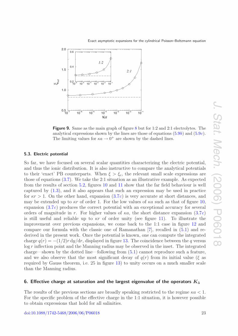
Figure 9. Same as the main graph of figure 8 but for 1:2 and 2:1 electrolytes. Theanalytical expressions shown by the lines are those of equations (5.9b) and (5.9c).The limiting values for κa → 0+ are shown by the dashed lines.

5.3. Electric potential

So far, we have focused on several scalar quantities characterizing the electric potential,and thus the ionic distribution. It is also instructive to compare the analytical potentialsto their ‘exact’ PB counterparts. When ξ > ξc, the relevant small scale expressions arethose of equations (3.7). We take the 2:1 situation as an illustrative example. As expectedfrom the results of section 5.2, figures 10 and 11 show that the far field behaviour is wellcaptured by (1.3), and it also appears that such an expression may be used in practicefor κr > 1. On the other hand, expansion (3.7c) is very accurate at short distances, andmay be extended up to κr of order 1. For the low values of κa such as that of figure 10,expansion (3.7c) produces the correct potential with an exceptional accuracy for severalorders of magnitude in r. For higher values of κa, the short distance expansion (3.7c)is still useful and reliable up to κr of order unity (see figure 11). To illustrate theimprovement over previous expansions, we come back to the 1:1 case in figure 12 andcompare our formula with the classic one of Ramanathan [7], recalled in (5.1) and re-derived in the present work. Once the potential is known, one can compute the integratedcharge q(r) = −(1/2)r dy/dr, displayed in figure 13. The coincidence between the q versuslog r inflection point and the Manning radius may be observed in the inset. The integratedcharge—shown by the dotted line—following from (5.1) cannot reproduce such a feature,and we also observe that the most significant decay of q(r) from its initial value (ξ asrequired by Gauss theorem, i.e. 25 in figure 13) to unity occurs on a much smaller scalethan the Manning radius.

6. Effective charge at saturation and the largest eigenvalue of the operators Ka

The results of the previous sections are broadly speaking restricted to the regime κa < 1.For the specific problem of the effective charge in the 1:1 situation, it is however possibleto obtain expressions that hold for all salinities.

doi:10.1088/1742-5468/2006/06/P06018 23

J.Stat.M

ech.(2006)

P06018

Exact asymptotic expansions for the cylindrical Poisson–Boltzmann equation

10–3

10–2

10–1

100

101

κr

0

10

20y 21

(r)

0 1 2 3 4 5κr

10–2

10–1

100

101

y 21

Figure 10. Electrostatic potential in a 2:1 electrolyte as a function of radialdistance for a rod with a high bare charge (ξ 11) and κa = 10−3. The circlesrepresent the numerical solution of PB theory, the dotted line is for the shortdistance formula (3.7c) and the dashed line is for the far field expression (1.3).In the inset, the same results are shown on a linear–log scale.

0 1 2 3 4κr

0

1

2

3

4

5

6

7

8

9

y 21(r

)

0 1 2 3 4 5κr

10–2

10–1

100

101

y 21

Figure 11. Same as figure 10 but with ξ 40 and κa = 0.3, on a linear scale.

The effective charge at saturation, for any arbitrary value of a, has an interestingrelation with the largest eigenvalue of the operators defined in equations (2.3) and (2.6).To see this, consider first the 1:1 electrolyte, and the solution (2.2) to the Poisson–Boltzmann equation. As the bare charge ξ increases the parameter λ (related to theeffective charge ξeff) increases. At saturation (ξ → +∞), λ = λsat is such that theelectric field obtained from the solution (2.2) diverges at r = a. Clearly this happens ifdet(1 − λKa) = 0, and thus if λ is the inverse of an eigenvalue of Ka.

7 Now, since when

7 This analysis is for (positive) saturation when ξ > 0. In the case ξ < 0, the saturation is reached whendet(1 + λKa) = 0.

doi:10.1088/1742-5468/2006/06/P06018 24

J.Stat.M

ech.(2006)

P06018

Exact asymptotic expansions for the cylindrical Poisson–Boltzmann equation

10–3

10–2

10–1

100

κr

0

10

20y 11

(r)

PB solution this work Ramanathan

Figure 12. Comparison of the numerical solution of PB theory withexpansion (3.7a) shown by the dotted line and with the formula of Ramanathan(see (5.1) and dashed line) for κa = 10−3, ξ = 25 and a 1:1 salt.

10–3

10–2

10–1

100

κr

0

5

10

15

20

25

q(r)

10–3

10–2

10–1

100κr

0.0

1.0

2.0

q(r

)

Figure 13. Integrated charge as a function of rescaled distance for the sameparameters as in figure 12 (symbols and lines have the same meaning here).The inset shows the same data in the vicinity of the predicted Manning radius,indicated by the arrow. The prediction follows from (5.6a) or equivalently (5.7a)since we consider here a highly charged rod.

ξ = 0, λ = 0 and it increases as ξ increases, it appears that at saturation λ = λsat is equalto the inverse of the largest eigenvalue of Ka.

The same analysis applies to the 1:2 and 2:1 electrolytes. For a 1:2 electrolyte, for

positive saturation ξ → +∞, λsat is the inverse of the largest eigenvalue of K(2)a , whereas

for a 2:1 electrolyte, when ξ → +∞, λsat is the inverse of the largest eigenvalue of −K(0)a .

We have not been able to find explicitly the eigenvalues of the operators Ka, K(0)a

and K(2)a , for any arbitrary value of a. However one can use approximate methods to find

estimates for the largest eigenvalue.

doi:10.1088/1742-5468/2006/06/P06018 25

J.Stat.M

ech.(2006)

P06018

Exact asymptotic expansions for the cylindrical Poisson–Boltzmann equation

For the 1:1 electrolyte, it is shown in the appendix of [37] that for any function

φ ∈ L2(0,∞, e−a(u+u−1)/2 du), the largest eigenvalue λ−1sat of Ka satisfies

(φ, Kaφ)

(φ, φ)≤ λ−1

sat (6.1)

where (· , ·) is the scalar product of L2(0,∞, e−a(u+u−1)/2 du). Using the test functionφ(u) = 1/

√u, we obtain

λsat ≤K0(a)

πΓ(0, 2a)(6.2)

with K0 the modified Bessel function and Γ(0, z) =∫ +∞

ze−t/t dt. Using equation (2.8a),

this finally gives an upper bound for the effective charge at saturation, for a 1:1 electrolyte,for any arbitrary value of a, ξsat

eff ≤ ξsat,up, with

ξsat,up =2aK1(a)K0(a)

π Γ(0, 2a). (6.3)

As a → 0, ξsat,up → 2/π, and thus has the same limit as the exact ξsateff . This is expected

since in the appendix [37], this upper bound was used to prove that the supremum of thelargest eigenvalue of Ka as a → 0 is π.

Interestingly, when a 1 we have

ξsat,up = 2a + 32

+ O(a−1) (6.4)

which is the same asymptotic behaviour as for the true effective saturated charge ξsateff

obtained in [38] by a and approach different to the present one. It is the effective chargeof an infinite plane (2κa) plus a correction (3/2) that is obtained using a small curvatureexpansion.

Figure 14 shows a comparison between ξsat,up from equation (6.3) and the effectivecharge at saturation ξsat

eff obtained numerically. Surprisingly, it turns out ξsat,up is notonly an upper bound for ξsat

eff but also a very good estimate for ξsateff for any value of a. If

a > 10−1 it is in very good agreement with the numerical data. However, for very smallradius a 1, the estimate (5.9a) of section 5.2, is better than the ansatz (6.3) (see theinset of figure 14 and compare it to figure 8).

7. Conclusion

The mathematical results derived in the framework of Painleve/Toda type equationsprovide much insight into the screening behaviour of microions in the vicinity of a chargedrod-like macroion. Although the mapping between the Poisson–Boltzmann equation fora certain class of electrolytes (1:1, 1:2 and 2:1) onto a Painleve/Toda equation is initself not new, previous analyses were concerned with the no salt limit where the ratioof macroion radius a to Debye length κ−1 vanishes, and the practical consequences andimplications of a finite salt concentration had not been drawn. We have shown here thatsystematic logarithmic, and thus strong, corrections arise for various quantities of interest.All finite salt results reported here are new, and significantly improve previously availableexpressions. In addition, the 2:1 situation worked out here had not been considered before,even in the limit of vanishing salt content.

doi:10.1088/1742-5468/2006/06/P06018 26

J.Stat.M

ech.(2006)

P06018

Exact asymptotic expansions for the cylindrical Poisson–Boltzmann equation

10–4

10–3

10–2

10–1

100

κa

0.0

2.0

4.0

6.0

8.0

ξsat,u

p

10–6

10–5

10–4

10–3

10–2

10–1

κa0.5

0.7

0.9

1.1

1.3

ξsat,u

p

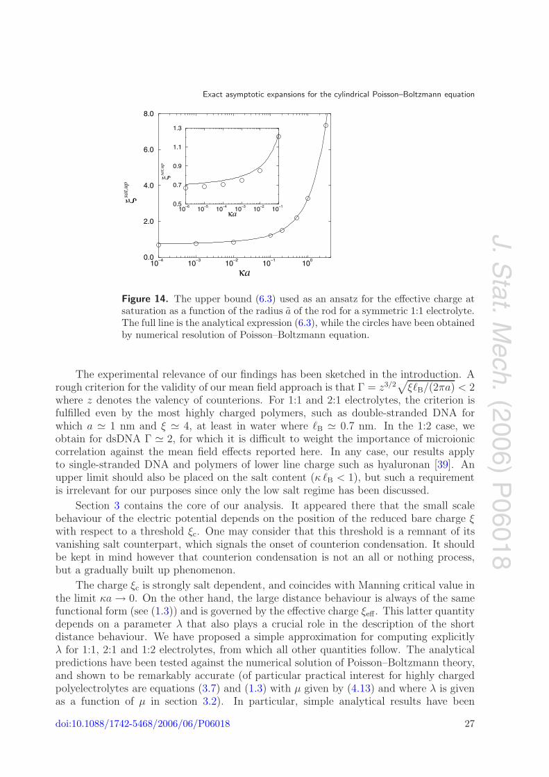
Figure 14. The upper bound (6.3) used as an ansatz for the effective charge atsaturation as a function of the radius a of the rod for a symmetric 1:1 electrolyte.The full line is the analytical expression (6.3), while the circles have been obtainedby numerical resolution of Poisson–Boltzmann equation.

The experimental relevance of our findings has been sketched in the introduction. Arough criterion for the validity of our mean field approach is that Γ = z3/2

√ξB/(2πa) < 2

where z denotes the valency of counterions. For 1:1 and 2:1 electrolytes, the criterion isfulfilled even by the most highly charged polymers, such as double-stranded DNA forwhich a 1 nm and ξ 4, at least in water where B 0.7 nm. In the 1:2 case, weobtain for dsDNA Γ 2, for which it is difficult to weight the importance of microioniccorrelation against the mean field effects reported here. In any case, our results applyto single-stranded DNA and polymers of lower line charge such as hyaluronan [39]. Anupper limit should also be placed on the salt content (κ B < 1), but such a requirementis irrelevant for our purposes since only the low salt regime has been discussed.

Section 3 contains the core of our analysis. It appeared there that the small scalebehaviour of the electric potential depends on the position of the reduced bare charge ξwith respect to a threshold ξc. One may consider that this threshold is a remnant of itsvanishing salt counterpart, which signals the onset of counterion condensation. It shouldbe kept in mind however that counterion condensation is not an all or nothing process,but a gradually built up phenomenon.

The charge ξc is strongly salt dependent, and coincides with Manning critical value inthe limit κa → 0. On the other hand, the large distance behaviour is always of the samefunctional form (see (1.3)) and is governed by the effective charge ξeff . This latter quantitydepends on a parameter λ that also plays a crucial role in the description of the shortdistance behaviour. We have proposed a simple approximation for computing explicitlyλ for 1:1, 2:1 and 1:2 electrolytes, from which all other quantities follow. The analyticalpredictions have been tested against the numerical solution of Poisson–Boltzmann theory,and shown to be remarkably accurate (of particular practical interest for highly chargedpolyelectrolytes are equations (3.7) and (1.3) with µ given by (4.13) and where λ is givenas a function of µ in section 3.2). In particular, simple analytical results have been

doi:10.1088/1742-5468/2006/06/P06018 27

J.Stat.M

ech.(2006)

P06018

Exact asymptotic expansions for the cylindrical Poisson–Boltzmann equation

derived for the Manning radius, that is often used to quantify the lateral extension ofthe condensate that may form around a cylindrical polyion. A few other measures of thecondensate thickness have been commented upon.

Our approach is free of the matching procedures [40]–[42] or ad hoc though educatedassumptions [43] underlying previous work, and therefore provides expansions withcontrolled error for the electric potential. The analysis of sections 3–5 requires thata < κ−1. For larger salinities, contributions that have been neglected here becomerelevant. However, the spectral analysis of section 6 provides for all values of κa an upperbound for the far field signature of the polyion, from which an excellent approximation ofthe effective charge at saturation may be obtained.

The analytical results obtained emphasize the essential difference between the criticalManning charge for condensation and effective charge of the macroion, the latter beingdefined from the large scale electric behaviour. A consequence is that within a simplifiedtwo-state model where the population of microion is divided into a condensed region anda free population, free ions cannot be treated within a linearized theory, at variance withcommon belief and practice. Consistency with exact results requires that non-linear effectsare still at work in the free region and significantly decrease the effective charge comparedto the critical one. In the 1:2 case at ultralow salt, for all bare charges ξ larger than ξc,the ratio of ξeff to ξc (with ξc equal to ξManning here since κa → 0) is equal to

√3/π 0.55.

This ratio is closer to unity for 2:1 electrolytes [3√

3/(2π) 0.83], and intermediate fora 1:1 salt (2/π 0.64). We therefore emphasize that the distinction between bound andfree ions is not only arbitrary but also potentially misleading.

Acknowledgments

We would like to thank T Odijk for useful remarks. This work was supported by a ECOSNord/COLCIENCIAS action of French and Colombian cooperation. GT acknowledgepartial financial support from COLCIENCIAS grant 1204-05-13625 and from Comite deInvestigaciones de la Facultad de Ciencias de la Universidad de los Andes. This work wassupported in part by the NSF PFC-sponsored Center for Theoretical Biological Physics(Grants No PHY-0216576 and No PHY-0225630).

Appendix A: Painleve classification; a brief reminder

Polynomial non-linear differential equations of the form

A(x, y)d2y

dx2+ B(x, y)

dy

dx+ C(x, y)

(dy

dx

)2

+ D(x, y) = 0, (A.1)

where the functions A, B, C, D are polynomial in y and analytic in x, have been classifiedwith respect to the character of the singular points of the solutions. Of special interestare the equations for which branch points and essential singularities do not depend oninitial conditions (and hence the only movable singularities are poles). Fifty canonicaltypes of equations with the above property have been uncovered, most of which (44) areintegrable in terms of elementary functions. Solving the remaining six types requires theintroduction of new (Painleve) transcendental functions. The third member (Painleve III)

doi:10.1088/1742-5468/2006/06/P06018 28

J.Stat.M

ech.(2006)

P06018

Exact asymptotic expansions for the cylindrical Poisson–Boltzmann equation

of this family of 6 corresponds to the generic form

xyd2y

dx2= x

(dy

dx

)2

− ydy

dx+ ax + by + cy3 + dx y4. (A.2)

Appendix B: Short distance behaviour for λ > λc

For a highly charged rod, when ξ > ξc, we have Re(A) = ξManning. Then, the last ‘higher’order terms in equations (3.5) become of the same order as the O(1) terms. Thus thesmall r asymptotics of y(r) are different, when ξ > ξc, to the ones given by equations (3.5).

In [22] the asymptotics for λ > 1 in the 1:1 case were studied and in [24] the ones forthe 1:2 case for λ > λc were obtained. We will not reproduce those calculations here, butto illustrate the method from [22, 24], we will compute the small r asymptotics for the 2:1

case, for λ > λ(2:1)c , which has not been previously considered.

The asymptotic form (3.5c) is actually valid even if λ is complex, provided that itsatisfies (3.14). To study the asymptotics when λ > λc we can consider that λ approachesthe cut [λc, +∞) from below, for instance. Then we can rewrite (3.13b) as

A = 1 − 32iµ (B.1)

with

µ =1

πln

√(3λ

2λc− 1

2

)2

− 1 − 1

2+

3λ

2λc

(B.2a)

=1

πcosh−1

(3λ

2λc− 1

2

)> 0. (B.2b)

Replacing into (3.5c) and keeping only the first two dominant terms (which are of thesame order) gives

e−y21/2 =−r

3√

6µi(z − z) + O(r8) (B.3)

with

z =

(r

6√

3

)3iµ/2 [Γ (1 − i(µ/2))Γ(1 − iµ)

Γ (1 + i(µ/2))Γ(1 + iµ)

]1/2

. (B.4)

If one chooses λ to approach the cut [λc, +∞) from above then µ is changed into −µ andthe final result is unchanged.

Finally, the potential y21 is given by

e−y21/2 =2r

3µ√

6sin

[−3µ

2ln

r

6√

3− Ψ(2:1)(µ)

]+ O(r8) (B.5)

where

Ψ(2:1)(µ) = Im

ln

[Γ

(1 − iµ

2

)Γ(1 − iµ)

]. (B.6)

doi:10.1088/1742-5468/2006/06/P06018 29

J.Stat.M

ech.(2006)

P06018

Exact asymptotic expansions for the cylindrical Poisson–Boltzmann equation

For the sake of completeness, we reproduce here small r asymptotics for the 1:1 andthe 1:2 cases which were computed in [22] and [24], respectively. For the 1:1 electrolyte,

when λ > λ(1:1)c , the electric potential is given by

e−y11(r)/2 =r

4µsin

[−2µ ln

r

8+ 2Ψ(1:1)(µ)

]+ O(r5) (B.7a)

with

µ =1

πcosh−1(πλ) > 0 (1:1) (B.7b)

and

Ψ(1:1)(µ) = Im [ln Γ(1 + iµ)] . (B.7c)

For the 1:2 electrolyte, when λ > λ(1:2)c , the asymptotics are [24]

e−y12(r) =r

3µ√

3sin

[−3µ ln

r

6√

3− 2Ψ(1:2)(µ)

]+ O(r4) (1:2) (B.8)

now with

µ =1

πcosh−1

(1

2+

λ

2λc

)> 0 (B.9)

and

Ψ(1:2)(µ) = Im

ln

[Γ

(1 − iµ

2

)Γ(1 − iµ)

]. (B.10)

For practical purposes, since µ is at most of order 1/| ln a|, we can expand the functions

Ψ(1:1)(µ) = −γµ + O(µ3) (B.11)

Ψ(1:2)(µ) = µ(

32γ + ln 2

)+ O(µ3) (B.12)

Ψ(2:1)(µ) = 3γµ/2 + O(µ3). (B.13)

The asymptotics presented in equations (3.7) in the main text use this approximation forΨ(µ).

In principle this means that our expressions in the main text for µ are accurate onlyto order O(1/| ln a|2). However, an explicit computation using further terms in the Taylorexpansion of Ψ(µ) shows that our results, in the form presented in the main text, areactually accurate up to order 1/| lna|3 for µ and order 1/| ln a|4 for the effective charges.

To illustrate this, consider, for example, the value of µsat for the 1:1 case. Using aTaylor expansion of Ψ(1:1)(µ) up to order µ3 gives

µ(1:1)sat =

π

2 ln(a/8)

[1 − γ

ln(a/8)+

γ2

(ln(a/8))2− γ3 + (π2/24)ψ(2)(1)

(ln(a/8))3

]+ O

((ln a)−5

)(B.14)

where ψ(x) = d ln Γ(x)/dx is the digamma function and ψ(2)(x) its second derivative.Replacing this expression into equations (3.12) and (2.8), yields the effective charge at

doi:10.1088/1742-5468/2006/06/P06018 30

J.Stat.M

ech.(2006)

P06018

Exact asymptotic expansions for the cylindrical Poisson–Boltzmann equation

saturation

ξ(1:1)sat = aK1(a)

[2

π− π3

4 (ln(a/8))2 +γπ3

2 (ln(a/8))3 +−144γ2π3 + π7

192 (ln(a/8))4

+π3(48γ3 − γπ4 + π2ψ(2)(1))/48

(ln(a/8))5 + O((ln a)−6

)]

. (B.15)

A direct comparison of equations (B.15) and (B.14) with (4.14a) and (5.9a) shows thatthe (more compact) expressions presented in the main text are indeed accurate up toorder 1/| ln a|3 for µ and order 1/| ln a|4 for ξsat.

References

[1] Khokhlov A, 2000 Soft and Fragile Matter (Scottish Graduate Textbook Series) ed M E Cates andM R Evans (Bristol: IoP)

[2] Manning G S, 1969 J. Chem. Phys. 51 924[3] Oosawa F, 1971 Polyelectrolytes (New York: Dekker)[4] Alfrey T Jr, Berg P W and Morawetz H, 1951 J. Polym. Sci. 7 543

Fuoss R M, Katchalsky A and Lifson S F, 1951 Proc. Nat. Acad. Sci. 37 579[5] Fixman M, 1979 J. Chem. Phys. 70 4995[6] Gueron M and Weisbuch G, 1980 Biopolymers 19 353[7] Ramanathan G V, 1983 J. Chem. Phys. 78 3223[8] Le Bret M and Zimm B H, 1984 Biopolymers 23 287[9] McCaskill J S and Fackerell E D, 1988 J. Chem. Soc., Faraday Trans. 84 161

[10] Kholodenko A L and Beyerlein A L, 1995 Phys. Rev. Lett. 74 4679[11] Tracy C A and Widom H, 1997 Physica A 244 402[12] Levin Y, 1998 Physica A 257 408[13] Deserno M, Holm C and May S, 2000 Macromolecules 33 199[14] Hansen P L, Podgornik R and Parsegian V A, 2001 Phys. Rev. E 64 021907[15] O’Shaughnessy B and Yang Q, 2005 Phys. Rev. Lett. 94 048302[16] Belloni L, 2000 J. Phys.: Condens. Matter 12 R549[17] Hansen J-P and Lowen H, 2000 Ann. Rev. Phys. Chem. 51 209[18] Grosberg A Y, Nguyen T T and Shklovskii B I, 2002 Rev. Mod. Phys. 74 329[19] Levin Y, 2002 Rep. Prog. Phys. 65 1577[20] Netz R R, 2001 Eur. Phys. J. E 5 557

Naji A and Netz R R, 2003 Eur. Phys. J. E 13 43[21] Levin Y, Trizac E and Bocquet L, 2003 J. Phys.: Condens. Matter 15 S3523[22] McCoy B M, Tracy C A and Wu T T, 1977 J. Math. Phys. 18 1058[23] Widom H, 1997 Commun. Math. Phys. 184 653[24] Tracy C A and Widom H, 1998 Commun. Math. Phys. 190 697[25] Trizac E and Tellez G, 2006 Phys. Rev. Lett. 96 038302[26] See e.g. Davis H T, 1962 Introduction to Nonlinear Differential and Integral Equations (New York: Dover)[27] Benham C J, 1983 J. Chem. Phys. 79 1969[28] Samaj L and Travenec I, 2000 J. Stat. Phys. 101 713[29] Cornu F and Jancovici B, 1987 J. Stat. Phys. 49 33[30] Odijk T, 1983 Chem. Phys. Lett. 100 145[31] Trizac E, Bocquet L, Aubouy M and von Grunberg H H, 2003 Langmuir 19 4027[32] Tellez G and Trizac E, 2004 Phys. Rev. E 70 011404[33] Tellez G and Trizac E, 2003 Phys. Rev. E 68 061401[34] Netz R R and Joanny J-F, 1998 Macromolecules 31 5123[35] Weisbuch G and Gueron M, 1981 J. Phys. Chem. 85 517[36] Qian H and Schellman J A, 2000 J. Phys. Chem. B 104 11528[37] Tracy C A, 1991 Commun. Math. Phys. 142 297[38] Aubouy M, Trizac E and Bocquet L, 2003 J. Phys. A: Math. Gen. 36 5835[39] Buhler E and Boue F, 2004 Macromolecules 37 1600[40] MacGillivray A D and Winkleman J J Jr, 1965 J. Chem. Phys. 45 2184[41] Philip J R and Wooding R A, 1970 J. Chem. Phys. 52 953[42] van Keulen H and Smit J A M, 1995 J. Colloid Interface Sci. 170 134[43] Tuinier R, 2003 J. Colloid Interface Sci. 258 45

doi:10.1088/1742-5468/2006/06/P06018 31