- 1 -

ESTIMATION AND TESTING OF

DYNAMIC ECONOMETRIC MODELS FROM PANEL DATA

by

Manuel Arellano Gonzalez

1985

Thesis submitted for the degree of

Doctor of Philosophy

at the

London School of Economics

Univexsity of London

- 2 -

This thesis is dedicated to my parents.

- 3 -

ABSTRACT

This research develops methods of estimation and test statistics

of dynamic single equation models from panel data when the errors are

serially correlated. It is assumed that the number of time periods

is fixed while the number of cross-section observations is large.

This makes it possible to consider prediction equations of the initial

observations based on the exogenous variables corresponding to all

periods available in the sample, as well as to leave unrestricted the

covariances of the prediction errors with the remaining errors in

the model.

The concentrated likelihood function is derived both for cases where

the prediction error is left unrestricted and where it is assumed to

have the marginal distribution of the stationary process. The performance

of maximum likelihood methods is investigated, either for correct models

or under several misspecifications, by resorting to Monte Carlo methods

using antithetic variates.

Dynamic models from panel data can be seen as a specialisation

of a triangular system with covariance restrictions. In this context,

the asymptotic distribution of the estimators that maximise the gaussian

likelihood function is derived when normality holds and also when the

errors are non-normal. In particular, it is shown that in the latter case

the estimator that takes into account the covariance restrictions

is not generally more efficient than the estimator that leaves the co­

variance matrix unrestricted.

The possibility of obtaining consistent estimates of the unrestricted

intertemporal covariance matrix is used to develop test statistics of

covariance restrictions arising from various random effects specifications.

A Wald test and a minimum chi-square test, which are robust to the non­

normality of the errors, and appropriate asymptotic probability limits

for the quasi-likelihood ratio test are proposed. Monte Carlo experiments

are conducted to study the performance of these test criteria. In order

to illustrate these procedures, QML estimates of dynamic earnings functions

from the Michigan Panel are obtained.

- 4 -

Joint minimum distance estimators of slope and covariance

parameters are defined that are generally efficient relative to QML

estimators when normality is not imposed and the covariance matrix

is restricted. Finally, it is shown that there exist separate

minimum distance estimators of the covariance parameters and generalised

least squares estimators of the slope parameters that are efficient.

A simulation is also carried out to examine the performance of these

methods.

- 5 -

ACKNOWLEDGEMENTS

I wish to thank my supervisor Professor J.D. Sargan for his

constant help, advice and encouragement. His many comments and suggestions

have been a constant source of inspiration for which I am particularly

grateful. But above all I must express my gratitude to Professor Sargan

for all I have learnt from him throughout the whole period of my research

which has profoundly influenced my understanding of econometrics.

Special thanks are due to Olympia Bover for her help, encouragement

and patience during the three years in which I worked on this thesis.

I have benefited from innumerable discussions with Olympia and her

careful reading of the manuscript has also led to numerous improvements

for which I am most grateful.

I am indebted to various other people for assistance in the prepar­

ation of this thesis. I thank A. Bhargava for the use of his maximum

likelihood computer program at the early stages of my work; G. Chowdhury

for making her data base available; and F. Srba for allowing me to go

through the program NAIVE and for his readiness to help. I am especially

grateful to J. Magnus for his help and useful comments. I would also

like to thank S. Peters and S. Marwaha for their help in my computing

work.

Financial support from the London School of Economics in the form

of a Suntory-Toyota Scholarship, the Caja de Ahorros de Barcelona and

the ESRC DEMEIC Econometric Project at L.S.E. is gratefully

acknowledged.

Finally, I am very happy to thank Christine Wills for typing the

bulk of the manuscript and ~1arianna Tappas for typing Chapter 4 in such

an efficient way.

- 6 -

CONTENTS

ABSTRACT

ACKNOWLEDGEMENTS

CHAPTER 1 DYNAMIC ECONOMETRIC MODELS FROM PANEL DATA

1.1 Introduction

1.2 The Model of Interest

1.3 The Problem of the Initial Observations

1.4 Estimating Models with Unrestricted Prediction

Equation for YiO

1.5 Serial Correlation and Unrestricted Intertemporal

Covariance

1.6 Correlation between the Explanatory Variables

and the Individual Effects

Notes

CHAPTER 2 QML ESTIMATION OF DYNAMIC MODELS WITH SERIALLY

CORRELATED ERRORS

2.1 Introduction

2.2 Three Alternative Models with ARMA Errors

2.3 Quasi-Maximum Likelihood Estimation

2.4 Estimation with Arbitrary Intertemporal Covariance

2.5 Experimental Evidence

2.6 A Model with Arbitrary Heteroscedasticity Over Time

Notes

3

5

9

10

12

19

24

28

36

38

39

43

52

55

61

70

Appendix 2.A The Determinant and the Inverse of the

Covariance Matrix for the Stationary ARMA(l,l) Process 71

CHAPTER 3 THE ASYMPTOTIC PROPERTIES OF QML ESTIMATORS IN A

TRIANGULAR MODEL WITH COVARIANCE RESTRICTIONS

3.1 Introduction

3.2 The Model and the Limiting Distribution of the

QML Estimator

3.3 The Asymptotic Variance Matrix of the QML Estimators

when the Errors are Normal

74

75

83

- 7 -

3.4 The Asymptotic Variance Matrix of the QML Estimators

when the Errors are Possibly Non-normal

3.5 A Simple Two Eqnation Model

Notes

Appendix 3.A The First and Second Derivatives of the

Quasi-log-likelihood Function with respect to e and T,

and the Matrices ~ , ~ , e , e and ~-lu r u r u

Appendix 3.B Derivation of Wr,ll and Wr ,22

88

94

101

102

110

CHAPTER 4 WALD AND QUASI-LIKELIHOOD RATIO TESTS OF RANDOM EFFECTS

SPECIFICATIONS IN DYNAMIC MODELS

4.1 Introduction 114

4.2 The AVM of ~-Unrestricted QML Estimators for Panel Data 115

4.3 Wald and Quasi-Likelihood Ratio Tests 119

4.4 Simulation Results 123

4.5 Estimation of Earnings Funct-ions for the us 125

Notes

CHAPTER 5 MINIMUM DISTANCE AND GLS ESTIMATION OF TRIANGULAR MODELS

WITH COVARIANCE RESTRICTIONS

5.1 Introduction

5.2 Joint Minimum Distance Estimation of Slope and

Covariance Parameters

139

141

143

5.3 The Asymptotic Variance Matrix of the Optimal Joint MDE 149

5.4 Efficient MDE of Covariance Parameters and Minimum Chi-

Square Specification Tests of Covariance Constraints

5.5 Generalised Least Squares Estimation of Regression

Coefficients

5.6 Subsystem Estimation

Notes

Appendix 5.A The Limiting Distribution of the Minimum Distance

Estimator

152

155

161

166

169

- 8 -

CHAPTER 6 EFFICIENT MD AND GLS ESTIMATORS APPLIED TO PANEL DATA

6.1 Introduction 171

6.2 The Estimators 172

6.3 Numerical Results 178

CONCLUSION 187

REFERENCES 189

- 9 -

CHAPTER 1

DYNAMIC ECONOMETRIC MODELS FROM PANEL DATA

1.1 Introduction

The dynamic error components mOdel has been a major subject of

attention for econometricians ever since economists began to make use

of panel data to estimate economic relationships. A reason why this

interest has so scarcely materialised in applied work is that, despite

recent relevant contributions, a complete answer to the problem of

estimating and testing dynamic models from panel data still does not

exist. It is the purpose of this rcscarch to present a further

contribution to this end.

The fact that typically a panel involves a large number of

individuals, but only over a short number of time periods, makes it

necessary to rely only upon the increase in the number of individual

units in developing the asymptotic properties of the statistical methods

under consideration. Treating the number of time periods as fixed

creates different problems to those encountered in time series analysis,

particularly a careful specification of initial conditions is required,

but it is also the basis of new and fruitful ways of approaching

dynamic modelling.

In what follows we introduce the dynamic error components model,

and we will survey the relevant literature as we discuss the implications

of different assumptions concerning the specification of the basic

equation.

- 10 -

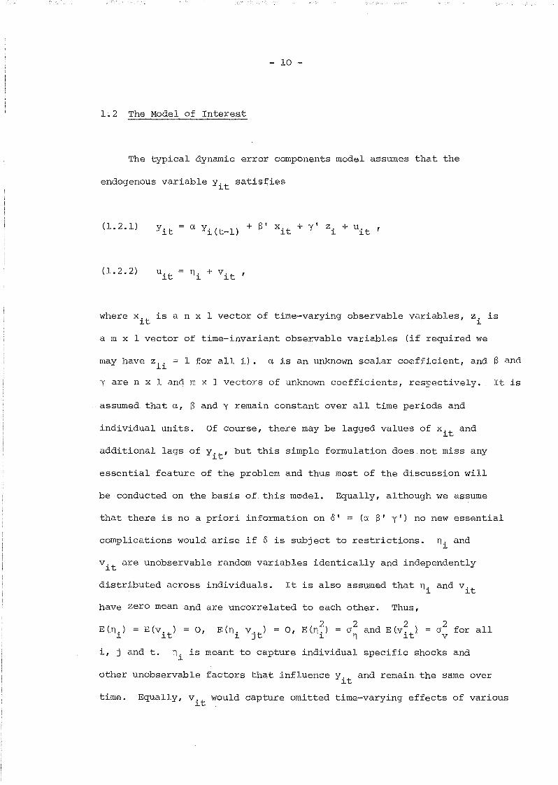
1.2 The Model of Interest

The typical dynamic error components model assumes that the

endogenous variable Yit satisfies

(1.2.1)

(1.2.2)

where xit

is a n x 1 vector of time-varying observable variables, zi is

a m x 1 vector of time-invariant observable variables (if required we

may have zli = 1 for all i). a is an unknown scalar c00fficient, and f3 and

y are n x 1 and m x 1 vectors of unknown coefficients, respectively. It is

assumed that a, 13 and y remain constant over all time periods and

individual units. Of course, there may be lagged values of xit

and

additional lags of Yit' but this simple formulation does not miss any

essential feature of the problem and thus most of the discussion will

be conducted on the basis of this model. Equally, although we assume

that there is no a priori information on 8' = (a 13' y') no new essential

complications would arise if 8 is subject to restrictions. ni

and

vit

are unobservable random variables identically and independently

distributed across individuals. It is also assumed that ni

and vit

have zero mean and are uncorrelated to each other. Thus,

E(n.) = E(V.t

) = 0, E(n. v.t

) = 0, E(n~) = 02

and E(VJ.~t)J. J. J.J J. n

2o for all

v

i, j and t. ni

is meant to capture individual specific shocks and

other unobservable factors that influence Yit and remain the same over

time. Equally, vit

would capture omitted time-varying effects of various

- 11 -

kinds that we assume can be well represented by a random error with the

same properties for different individuals, though the effects embodied in

vit

can induce serial correlation. We could also assume a time specific

component in uit

' but as we shall consider inference for a fixed

number of time observations, it will not be a problem to condition on

the time specific effects that are in the sample if desired (by treating

them as a further set of coefficients to be estimated), and therefore

we omit them for simplicity in this general discussion.

There remains the question of what properties to attribute to the

observable variables x. and z.. The simplest possibility is to~t ~

assume that xit and zi are stochastic variables independent of uit .

In this case we would be conducting inference conditional on the

values of xit and zi that are in the sample, and so there is no

difference if we regard these sample values as being fixed. Moreover,

this provides a more natural framework since we shall encounter many cases

where some exogenous variables cannot be considered as random. Indeed,

this is the assumption that We shall make throughout the remaining

chapters of this work. However, if we think of n. as a latent variable~

representing relevant but unobserved characteristics, it would be

reasonable to assume that some or all the observed explanatory variables

are correlated with n .. This situation has been extensively studied~

for static models in the literature (cf. Mundlak (1978) and Hausman

and Taylor (1981), among others). In fact, some authors would point

to the ability of controlling unobserved individual heterogeneity as

one of the main purposes in using panel data. This point will be

discussed further in Section 1.6.

- 12 -

We assume that our sample consists of N individual units (i=l, •.• ,N)

observed through (T+l) consecutive time periods (t=O,l, ... ,T).

Nevertheless, there is no reason to believe that the process of the

dependent variable started at the same time at which we started

sampling, and even in this case it would be unreasonable to assume that

the individual effects ni did not play a role in determining YiO'

If lal<l and the process of Yit started in the distant past, our

model implies the following equation for YiO

(1.2.3)co

I ak

a' xi (-k) + Y*' Zi + nr + vIok=O

-1 -1with y* = (l-a) y, n~ = (l-a) n. and v~O

111

It is the presence of time-varying exogenous

co

\' a kL vi (-k) .

k=Ovariables in our original

equation what complicates matters, as it makes YiO to depend on the

entire past history of such variables. In this sense, even if we know

the distribution of uit

' further assumptions about the initial observat-

ions are required to be able to define maximum likelihood estimators

of (a a y). In the next Section we shall discuss different solutions that

have been proposed in the literature to circumvent this problem and

their implications for panel data.

1.3 The Problem of; the Initial Observations

If we complete the model (1. 2 .1) by assuming that the values of

YiO are fixed for all i, xit and zi are nonstochastic and there is no

serial correlation among the vit

' we have the model of Balestra and

- 13 -

Ner10ve (1966). Further assuming that the uit

are normally distributed,

Balestra and Nerlove defined the maximum-likelihood estimator and also

a generalised least squares estimator (the 'two round' estimator).

This model and related estimation methods have been the object of

detailed analysis in a series of Monte Carlo studies by Nerlove and

Maddala (cf. Nerlove (1967), Nerlove (1971) and Maddala (1971)). The

difficulty here is that these methods of estimation will only be

consistent (as N + 00) if the YiO are truly fixed or stochastic but

independent of n.; otherwise they will fail to control for the lack~

of orthogonality between YiO and uil in the equation for Yir.

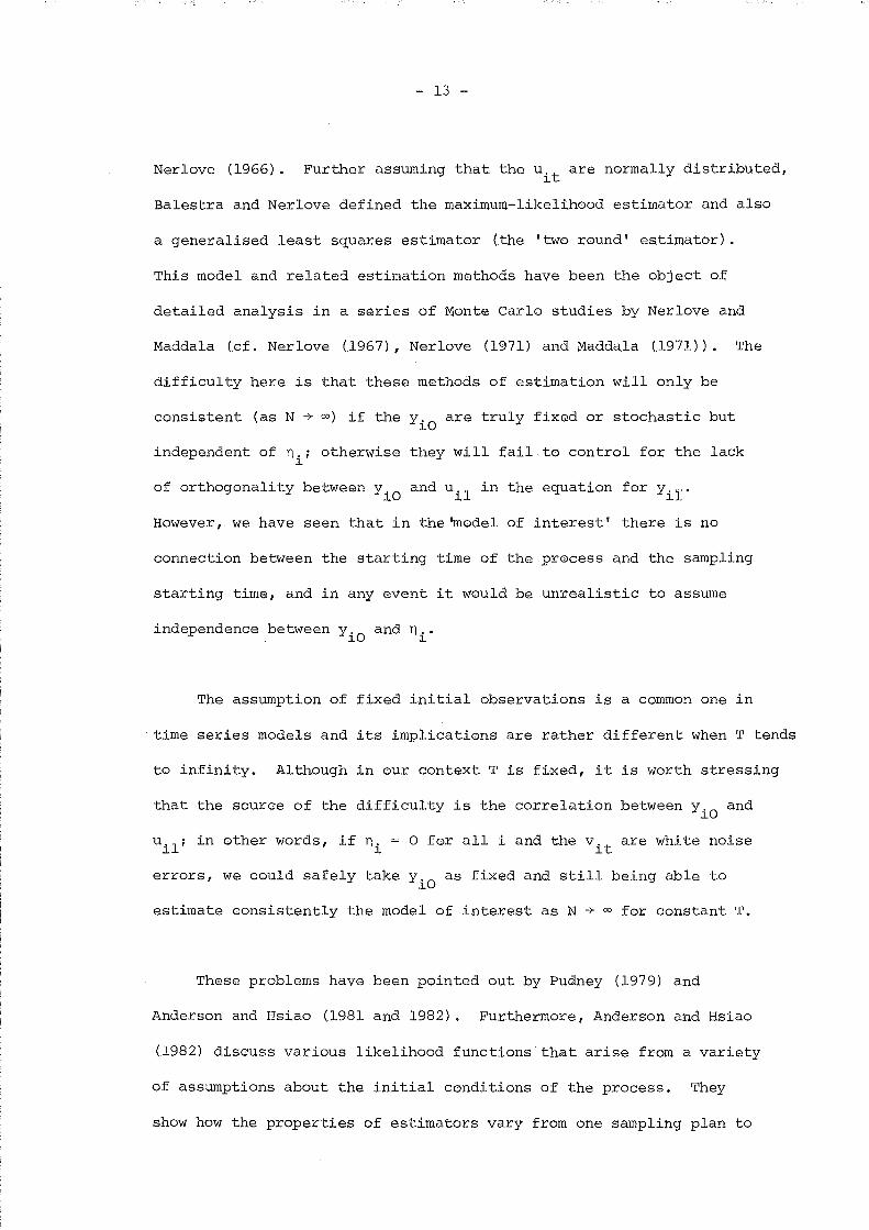
However, we have seen that in the 'model of interest' there is no

connection between the starting time of the process and the sampling

starting time, and in any event it would be unrealistic to assume

independence between y.O and n .•~ ~

The assumption of fixed initial observations is a common one in

time series models and its implications are rather different when T tends

to infinity. Although in our context T is fixed, it is worth stressing

that the source of the difficulty is the correlation between YiO and

u. l ; in other words, if n. = 0 for all i and the v. are white noise~ ~ ~t

errors, we could safely take y. as fixed and still being able to~O

estimate consistently the model of interest as N + 00 for constant T.

These problems have been pointed out by Pudney (1979) and

Anderson and Hsiao (1981 and 1982). Furthermore, Anderson and Hsiao

(1982) discuss various likelihood functions that arise frOm a variety

of assumptions about the initial conditions of the process. They

show how the properties of estimators vary from one sampling plan to

- 14 -

another and also depend on the way in which the sample becomes large

(N + 00 or T + 00). However, it would be useful to discuss the relative

merits of different assumptions about the initial observations as

approximations to what we call the model of interest.

The solution adopted in this work is to complete the system in

Section 1.2 with an unrestricted prediction equation of the form

(1.3.1) +)1. I X + +)1' x + ~I Z + Uo iO ••. T iT S i iO (i=l, ... ,N).

This alternative has been advocated by Bhargava and Sargan (1983)

and Chamberlain (1984), although rationalising equation (1. 3.1) in

different frameworks. On the one hand, Chamberlain assumes

(y~ x~ z~) where y~ = (y y) x' - (x' x') to be1. 1. 1. 1. iO' ... , iT' i - iO' ... , iT'

independent and identically distributed according to some common

multivariate distribution with finite moments up to the fourth order.

Under this sole assumption there is no reason a priori for the

regression function E(y'olx" z,) to be linear, but a minimum mean-1. 1. 1.

square error linear predictor can always be specified

E*(y'Olx., z,)1. 1. 1. Yio' say.

Furthermore, if E (y , 0 Ix" z,) t- E* (y, 0 Ix., z,), U +1.'0 will be heteroscedastic,1. 1. 1. 1. 1. 1.

since it will contain {E(y'olx" z,) - E*(y Ix z)} On the other hand,1. 1. 1. iO i' i .

Bhargava and Sargan assume uit

to be normally distributed, and xit

and

zi to be independent of uit

· Then if we let YiO

to be systematic

part of (1. 2 . 3)

- 15 -

00

I ()',k 13 I Xi (-k) + y*' zik==O

they assume yio to be the optimal predictor of YiO condition~l upon

d h * ' 1xi an zi' were €i YiO - YiO ~s a so

distributed for all i with variance 02

•€

normally and identically

These assumptions allow

+Bhargava and Sargan not only to ensure the homoscedasticity of uiO

but also to characterise the form of its variance and the covariances

with uil' ... ,uiT ; that is, since

(1.3.2) € + n~ + v*i ~ iO

if la\<l and vit is stationary we then have

(1.3.3) E (. +2)uiO

2o€

+

2o

_-..:.n_ + E (vi5)Cl-a) 2

(1.3.4)

2o

---1n + E(V~O V't)-a ~ ~(t==l, ... ,T) .

Furthermore, if vit is white noise (the case considered by Bhargava

and Sargan), E(vi~)2 2

0v/(l-a ) and E(vio v

it) == 0 for t==l, ... ,T.

In any event, notice that our model, once completed with the

prediction equation for y. above, can be written as~O

(1.3.5) u, (i==l, ... ,N)~

where B(a) is the (T+l) square matrix

- 16 -

1 a a a a

1-a 1 a a aB(a)

Ia a a . .-a 1

J

Cx

(ll,(3) is the (T+l) x (T+l)n matrix

ll'1

(3 ,

a

ll' )T

a

Cz(~'Y) is the (T+l) x m matrix

and u~l

The variance matrix of u. is given byl

(1.3.6) E (u. u ~ Ix" z.)l l l l

E(U:a2Ix.,z.) . E(U: u'llx.,z)l l l la l l ~

2(J 11' + V

11

J

where V is the variance matrix of (vil ..•v iT) and 1 is a T x 1 vector

of ones.

Thus our model can be expressed as a simultaneous triangular system

of T+l equations with linear restrictions linking the coefficients of the

last T equations. Indeed, since the parameters of interest (a, (3, y) are

- 17 -

confined to this subset of equations (the 'structural block') and the

prediction equation for YiO is unrestricted, explicit estimation of

the coefficients of the latter will not usually be required. We postpone

the discussion about the implications of the covariance matrix structure

to the next Section.

Nerlove (1971) and Pudney (1979) have proposed to use lagged values

of the exogenous variables as instruments for the lagged dependent

variable in order to ensure consistent estimation of the model of

interest. It has also been pointed out that, following this approach,

the best choice of instruments is not obvious, since the number of time

observations available depends upon the number of instrwilents chosen.

It is therefore of some interest to highlight the instrumental variables

implications of the unrestricted prediction equation for y. discussedlO

above.

The simplest consistent estimator of a set of equations in a

simultaneous system is well known to be the IV estimator that ignores

the fact that the covariance matrix is not a scalar matrix (what in the

absence of cross-equation restrictions is simply equivalent to 2SLS

estimation of separate equations). This is Sargan's Crude Instrumental

Variable estimator (CIV), and we can define the CIV estimator of

0' = (a S' y') for the block of the last T equations in the system

(1.3.5) by choosing 0CIV to

(1.3.7) -1min [vec (0)]' (Z* (z* I Z*) Z*, §:ll IT) vec (D)o

- 18 -

where U' = (ul u 2 ... uN)' Zi' = (xi, zi) and Z*' = [zi •.• z;].l

i.e. Z* is an N-rowed matrix of observations on the exogenous variables

with (T+l)n+m columns.

In order to relate 6CIV

to other estimators suggested in the

literature, let us introduce the following NT-vectors

we also define the NT x n matrix of time-varying exogenous variables

and the NT x ill matrix of time-invariant exogenous variables

Z ' [ z 1 ••. z1 •.• zN ... zN] .

Furthermore, introducing the NT x (n+m+l) matrix X+ = [Y-l

: X : Z],

we can write our structural block of T equations in the usual regression

form

(1.3.8) Y+X 6 + U •

- 19 -

Now, a simple explicit expression of 0CIV can be obtained by

noting that vec(U) = u. Then straightforward minimisation of

gives

(1.3.9)°CIV

Clearly, the matrix of instruments in regression form is the

NT x T [ (T+l) n+m] matrix (Z* ~ IT). This is an optimal set of instruments

in the absence of any prior knowilledge about the way in which the process

of Yit started off when T is fixed. Obviously, this requires Z* to be

of full column rank for identification and therefore if a subset of

variables in the vector xit

do not vary across individuals, they must

not be used as instruments in the definition of z*, although they will

be included in x+ (cf. Bhargava and Sargan (1982) for a discussion on

macro-variables) .

1.4 Estimating Models with unrestricted Prediction Equation for YiO

In this Section we survey the methods that have so far been proposed

for estimating models with unrestricted prediction equations for the

initial observations.

Under Chamberlain's assumptions E (u;-2Ix. ,z.) and E (u+l'0 u. t Ix. , z. )lO l l l l l

(t=l, .•• ,T) will be arbitrary functions of x. and z. and therefore, inl l

- 20 -

general, heteroscedastic. writing model (1.3.5) in reduced form we

have

(1.4.1) (px 1

z. J1.

+ V.1.

where P = (Px

-1C ) and V. = B (a) u.. The

Z 1. 1.

constraints in B, C and C imply a set of non-linear restrictions onx z

P. Let P be the unrestricted least squares estimator of P

N r N rP I y. z*' I I '7'.* z':<'i

~.

i=l1.

l i=l1. 1.

Allowing E(V. v~ Ix., z.) to be an arbitrary function of x. and z.,1. 1. 1. 1. 1. 1.

Chamberlain (1982 and 1984) follows White (1980) 's approach to show

that

A Dmvec(p-p) + N(O, W)

where

and

W-1 1

E [\!. \!' ~ M (z ':< z, ':< ' ) M- ]1. i 1. 1.

M E(Z~Z7')1. 1.

A consistent estimator of W can be obtained from the corresponding

sample moments

- 21 -

w

with

z* z*'i i

Then Chamberlain proposes to use a minimum distance procedure to impose

the nonlinear restrictions on P. That is, we minimise the following

criterion function with respect to the free parameters in p2

A_l[vec(P-P)] r w vec(P-P).

Alternatively, Chamberlain suggests to use the structural form and apply

a 'generalised three-stage least squares' estimator, which achieves

the same limiting distribution as the minimum distance estimator

sketched above; the advantage of the latter is that as the restrictions

in the structural form are linear there is no need to use numerical

methods of optimisation.

Under Bhargava and Sargan's assumptions, the variance matrix of the

error, ~* say, is fully specified and remains the same across individual

units. Relying upon the assumption of normality they specify the log-

likelihood function for the complete system

L k - ~ N log det(~*) -N

~ I u~ ~*":'l u.i=l

1. 1.

Bhargava and Sargan discuss two types of estimators. First, assuming ~*

to be an arbitrary (T+l)x(T+l). symmetric matrix, they consider the

- 22 -

likelihood function concentrated with respect to ~* and the coefficients

in the prediction equation ~ and ~ as an straightforward application

of the LIML method from the classical simultaneous equations theory.

Second, concentrating only ~ and ~ out of the likelihood function they

enforce on ~* the error components restrictions given by (1. 3 .3), Cl. 3.4)

and Cl.3.6). This likelihood function has to be maximised with the

restriction that laJ<l.

As it stands, the comparison of the two approaches suggests a

trade-off between robustness and efficiency. If the errors are truly

normally dis"tributed we may expect maximum likelihood estimators to

make an optimal use of the constraints in the covariance matrix, thus

leading to efficient estimators of all parameters in the model. However,

since in many practical situations there are no particular reasons to

assume normality (and frequently sample measures of skewness and kurtosis

will contradict this assumption) it is of interest to investigate the

properties of the estimators obtained by maximising the gaussian

likelihood function when the assumption of normality is false.

The early work from the Cowles Commission (cf. Koopmans, Rubin and

Leipnik (1950)) demonstrated that maximum likelihood estimators of the

simultaneous equations model with unrestricted covariance matrix

maintained the same asymptotic distribution even when the errors are

non-normal, and called them quasi-maximum likelihood (QML) estimators.

However, as the discussion in Chapter 3 will make it clear, this is not

the case in the presence of a priori knowledge about the covariance

matrix. In this situation, the QML estimator does not make optimal use

of the prior information and its asymptotic distribution depends on

- 23 -

higher order moments of the errors. Moreover, it will be shown that

it can be the case that the covariance restricted-QML estimator of the

slope coefficients is less efficient than the QML estimator that leaves

the covariance matrix unrestricted.

Chamberlain's procedure is very robust in the sense that by allow-

ing the reduced form errors variance matrix to be an arbitrary

function of x. and z., we can make consistent inferences about (a, S', y')~ ~

in a wide variety of situations. However, while there are no particular

reasons to believe that u~o is homoscedastic, the variance components

structure for uil, •.. ,uiT is one of the basic features of the model that

we are int.erested in test.ing. Moreove-r, if a structure of this kind

(possibly including an autoregressive-moving average scheme for the

transitory component vit

) is not rejected, the implied constraints can

be exploited in order to obtain more efficient estimates of (a, S', y').

In view of this consideratio~,we shall make the simplifying

+2 +assumption that E(u. ) and E(u, u. ), t=l, ..• ,T, do not depend upon

~O ~O ~t

z~ (possibly accompanied by a White (1980a) 's heteroscedasticity test),~

while assuming that (u~o uil' ... ,uiT) are independently and identically

distributed according to some multivariate distribution, not necessarily

normal, with finite moments up to the fourth order. Furthermore,

we can replace Bhargava and Sargan's stationarity assumptions about the

, b + dcovar~ances etween uiO

an uil, .•. ,uiT ' wOl

' w02 , .•. ,wOT say, by assuming

that they are a further set of T arbitrary coefficients. Note that the

+variance of u iO ' woo' is already effectively unrestricted in

2Bhargava and Sargan's formulation given the presence of 0. This

E:

- 24 -

approach has been introduced in Arellano (1983, 1984) and has various

3advantages. First, it allows us to consider nonst~tionary schemes

for the v. taking advantage of the availability of a large number ofl.t

observations per-period (see Section 1.5 below), and it also makes

unnecessary to restrict a to lie inside the unit circle. Second,

under this formulation, the error covariance matrix is constrained but

independent of the slope parameters, what will lead to enormously

simplified efficient methods of estimation for both regression and

covariance parameters (see Chapters 5 and 6). In particular, it is

worth noticing that in the QML context, it is possible to concentrate

Woo' wOl,···,wOT out of the likelihood function, thus leading to

simpler manipulation and lesser computational burden.

1.5 Serial Correlation and Unrestricted Intertemporal Covariance

The effect of random shocks acting through the time-varying

errors, while deteriorating over time, may persist longer than one

period. The vit may also include unobservable variables which are

serially correlated. Since both situations are likely to occur in

practice, it is unrealistic to make the assumption that the vit are

white noise errors. This fact has been acknowledged for a long time,

and many researchers have allowed for serial correlation - mostly first

order autoregressive schemes - in the estimation of st~tic equations

from panel data (ef. Lillard and Willis (1978), Bhargava, Franzini and

Narendranathan (1982), Chowdhury and Nickell (1982), and MaCu:r;dy (1982),

among others).

- 25 -

However, given the fact that T is fixed and N is la~ge we a~e able

to estimate arbitrary intertempo~al cova~iance matrices, thus ~voiding

4to place restrictions in the form of the serial co~relation of uit .

Therefore, if the objective is simply 'to allow for' serial correlation,

a robust solution is to obtain ~* unrestricted estimates of ~, Sand y.

The problem of specifying serial correlation in panel data then becomes

a problem of modelling ~* (for example, researchers can be inteJ:;'ested

in testing the existence and the magnitude of a permanent component

in the error term). A consequence of this is that it is possible to

consider a broader family of models than in time series models. Various

kinds of non-stationarity can be introduced, like autoregressive

schemes with the roots on or outside the unit circle, arbitrary forms

of time heteroscedasticity, or ARMA schemes with changing coefficients

(cf. MaCurdy (1982)). Nevertheless, it is convenient to preserve the

interpretability of the error structures under consideration and in

this regard the models that display a stationary correlation pattern

are the more interesting. Incidentally, notice that it is possible to

allow for arbitraryheteroscedasticity over time and at the Same time

to specify a stationary serial correlation pattern for vit

; this can

be achieved by setting

where Vit follows some stationary ARMA process with i.i.d. (0,1) white

noise errors. Now we have coy (v, t' V. ) = (J (J COV (v~ ,v~ ) and thusl lS t s It lS

Corr (v't'V, ) = Corr (v~t'v'I; ) foX" any i. This is not the case if wel lS l lS

consider instead an ARMA process where the variance of the white noise

error is varying over time. However, more general non-stationary models

- 26 -

are still possible, and see Ms.Curdy (1982) and Tiao and Ali (1971)

for suggestions about the treatment of initial conditions when stationary

correlation is not assumed.

MaCurdy (1982) has also proposed a method of selecting autoregressive­

moving average schemes for the vit

in models that are not dynamic.

His suggestion is to use least-squares residuals of the equation in

first differences (thus avoiding the complications originated by the time

invariant error component) to construct sample correlograms and sample

partial correlation functions, which can be used as a basis for choosing

an appropriate specification for the ARMA process generating the

transitory components. Then since differencingsimply introduces an

unit root in the moving average polynomial, its effects can be undone

in the sense that one can reconstruct the ARMA process associated with

levels. MaCurdy also suggests an ingenious method to estimate simple and

partial autocorrelations using a constrained seemingly unrelated equations

procedure. Once a particular specification is chosen, he proposes to

estimate the restricted cQvariance matrix by using conditional QML

methods (see also Ma'Curdy (1981) for a discussion of its properties) .

While this approach could be generalised to dynamic models (e.g.

by basing the calculation of correlograms on three-stage least-squares

residuals) and it can be of interest in indicating models to consider,

the possibility of obtaining consistent estimates of ~* unrestricted

suggests to base a formal specification search on a sequence of tests

of particular structures against ~* unrestricted in increasing order of

complexity. This is the approach advocated by Bhargava and Sargan (1983),

which rely upon likelihood ratio statistics to test the white noise error

- 27 -

components model against ~* unrestricted. Unfortunately, unlike the

case of regression parameters constraints, likelihood ratio tests

of covariance restrictions are asymptotically distributed as a chi-

squared on the null hypothesis only under the assumption of normality

of the error term (a point noticed by M~Curdy (1981) and that will be

discussed in Chapter 4). The asymptotic distribution of the

likelihood ratio test under the null hypothesis can still be calculated

when the errors are non-normal, but it seems convenient to construct

tests that are robust to the non-normality of the errors. Among these,

we shall develop Wald tests (Chapter 4) and minimum chi-square l tests

(Chapters 5 and 6). The advantage of the former is that it only

requires the estimation of the unrestricted model. However, as it is

well known there are two different ways of expressing exact prior

information. If W is the (T+l) (T+2)/2 vector of different elements

of ~*, a set of r constraints can be expressed as a set of equations

of the form

f. (w)J

o (j=l, ••• ,r) •

Alternatively, we may assume that the elements of ware related

functionally to a second set of (T+l) (T+2)/2-r parameters T

W=W(T).

Setting up Wald tests requires explicit expressions of the

constraint equations f. (j=l, .•. ,r) which can be difficult to obtain inJ

some cases. On the contrary, minimum chi-square· statistics are

- 28 -

expressed in terms of the constrained parameters T, what, ~or our

purposes, will usually be a straightforward way of handling the

problem.

1. 6 Correlation between the Explanatory Variables and the Individual

Effects

A leading objective in the estimation of models from panel data

has been to obtain estimates of the regression coefficients free of

bias due to the omission of relevant individual-specific effects. In

static models, this has traditionally been achieved by sUbtracting

time means to individual observations, thus removing all time-invariant

terms in the equation. Clearly, in this way the coefficients on the

time-invariant variables y cannot be estimated. In fact, if all the

xit

and zi are correlated with the individual effects, the y's are

not identified. Different alternatives arise if we are willing to

assume that some of the included explanatory variables are uncorrelated

with the individual effects. This is the case studied by Hausman and

Taylor (1981) for static models and Bhargava and Sargan (1983) for

dynamic models.

In the latter context, we still assume that xit

and zi are

independent of vit

but now we introduce the partitions

Xit = (xii t ; x 2i t) of dimension (1 x n l , 1 x n 2) and zi = (zli : z2i)

of dimension (1 x ml,l x ffi2

) such that xlit

and x2it

are, respectively,

vectors of variablesuncorrelated and correlated with the n., andI

similarly for zli and z2i. The suggestion of Hausman and Taylor is to

use the individual means of the xl' variables as instruments for theIt

- 29 -

z2i' and thus a necessary condition for the identification of 13 and '(

(in their model a is equal to zero) is that n l ~ m2 . If the rank

condition does not fail and nl

> m2

, the Hausman and Taylor1s

estimator of 13 differs from and is more efficient than the within-

groups estimator, while if nl

= m2

the two estimators are identical.

Incidentally, note that Hausman and Taylor1s reduced form equation for

z2i can be replaced by

(1.6.1)

Indeed, they assume ~O =... = ~T· These restrictions can be appropriate

if T is large and xlit is stationary, but in general they are not

justified in the present context (see Chamberlain (1980 and 1982) for

a discussion of this point). Using a general reduced form for z2i'

each variable in xlit

provides a set of T+l instruments for the z2i

and the order condition for identification becomes (T+l)nl~ m2 .

Bhargava and Sargan adopt a similar approach for dynamic models,

but they further assume that the deviations from time means of the

x 2it are uncorrelated with ni' what enables them to have a set of Tn2

extra instruments at the expense of only n 2 neW variables - the time

means of the x 2it - that are correlated with ni

. Let us consider

this model in some more detail. In general, we can write

(1.6.2) (t=O,l, •.. ,T)

where S. is independent of n ..It l

But if we assume KO

- 30 -

(1.6.3) (t=l, ..• ,T)

where x2i

1T+l

T

I x2it and ~it=o

1T+l

T

It=o

s. , so that the X 2 't are~t ~

independent, of Tl i . The vector of inst.rument.al variables is now

and the complete model can be expressed as

(1.6.4) B(ex) Yi + C x, + C Z, = u,x ~ Z l. l.

(1.6.5)+

f;:ziz2i F z. + ,l.

(1.6.6)+

!;xix2i G z. +l.

(1.6.7) (t=l, ... ,T) •

T .:.. 4, nl

> 0,

Substituting the last set of T identities into the first block of

equations, we obtain a system of (T+l) + m2 + n2 equations whose

+' -endogenous variables are given by y, = (y ~, z2'., x

2'.). The

l. l. l. l.

identification of this model, as shown by Bhargava and Sargan, requires

N + +'P lim(l;. l(z. z. )/N) to be positive definite and the

l.= l. l.

matrix Fx to be of full rank, where F =: (F : F ) and F correspondx z z

to the columns of cQefficients on zli' A crude instrumental variables

estimator of 0' =: (ex S' y'), equivalent to (1.3.9) minimises

(1.6.8)+ +' + -1 +'

[vec (U) ] I (z (z z) z· ~ IT) vec (U)

where

(1.6.9)

+'z

- 31 -

(z+ +) d' t' . b1 "",ZN ' an ~ ~s g~ven y

+' + +' + -1 +1 + -1 +1 + +' + -1 +'[x (z (z z) z ~ IT)X] x (Z (Z z) z ~ IT)y.

Using CIV residuals, uit

say, we can compute an unrestricted estimate

of the covariance matrix of (ui1 ' .•. ,uiT )

(1. 6.10) A {l NQ = - LN . 1

~=

(t,s=l, .•• ,T)

which in turn can be used to construct a three stage least-squares

estimator of °

(1.6.11) 03SLS

03SLS is asymptotically equivalent to the Q-unrestricted LIML estimator

suggested by Bhargava and Sargan. They also apply ,to this case the

constrained LIML procedures that enforce the error components

restrictions on the covariance matrix.

None of these methods can be applied when the individual effects

are suspected to be correlated with all the observed explanatory

variables. Regrettably, the within-group estimates for dynamic models

are inconsistent as N tends to infinity if T is kept fixed. Analytical

expressions for these inconsistencies have been given by Nickel1 (1981) •

The problem is that transformations like deviations from time means or

first differences fail to remove the correlation between the lagged

endogenous variables and the disturbance term. However, they do remOve

- 32 -

the permanent component of the errors and so the source of correlation

with the remaining explanatory va:r;iables. Thus, if proper account is

taken of the correlation between lagged y's and errors, consistent

estimation of the coefficients corresponding to time-varying variables

is still possible. But this is precisely the problem that the methods

introduced in Sections 1.3 and 1.4 are intended to solve, and they

can be easily extended to cover such cases.

For example, transforming to first differences our original

equation we have

(1.6.12)

(1.6.13) u*it

(t=2, .•. ,T).

Now, the model has to be completed with prediction equations for

YiO and Yil (see Chamberlain (1984))

(1.6.14) YiO

(1.6.15) Yil

If vit follows an ARMA(l,l) scheme with coefficients ~ and A , ult

will

follow an ARMA(l,2) scheme of the form

(1.6.16) u*it

- 33 -

2In particular, if v

itis white noise with variance 0 , the covariance

matrix of (ui2, •.• ,uiT) will be a (~-l) x (T-l) matrix of the form

( 2 -1 0 0 tI2

I-1 2 -1 0

20 0 ~o' say.

l I0 o ... -1 2

J

Since T is fixed, none of the time series problems that appear in the

estimation of models with moving average errors when the root lies

on the unit circle are relevant here. If the vit

are known to be

white noise errors, ~o can be used to construct a 3SLS estimator of

a and S by minimising

(1.6.17) S (a, S) [vec (U*)] I

where X' == (xl' •.. ,xN) and U*' == (ui' •• ·'u~) with ui' == (ui2,···,uiT).

Moreover, noting that vec(U*) == u* where u* is a N(T-l) x 1 vector of

errors in first differences

and that

u* (IN @ D)u

where u is defined in Section 1.3 and D is the (~-l) x T matxix

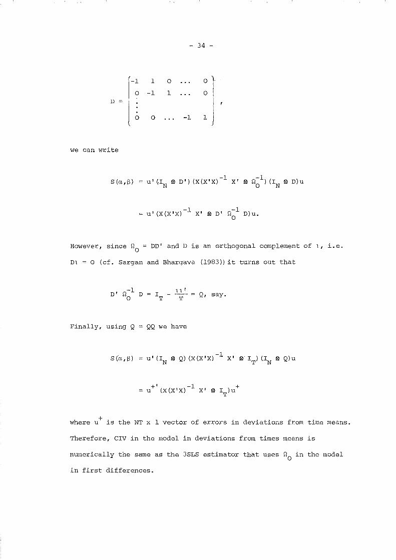
- 34 -

( -1 1 0 0 I0 -1 1 QD I

0 0 -1 1 J

we can write

Sea,S)-1 -1

u' (IN ~ D') (X(X'X) X' ~ rlo )(IN ~ D)u

However, since rlo = DD' and D is an orthogonal complement of 1, i.e.

D1 = 0 (cL Sargan and Bhargava (1983)) it turns out that

Q, say.

Finally, using Q

Sea,S)

QQ we have

+' -1 +u (X ex' X) X' ~ IT) u

where u+ is the NT x 1 vector of errors in deviations from time means.

Therefore, CIV in the model in deviations from times means is

numerically the same as the 3SLS estimator that uses rlo in the model

in first differences.

- 35 -

The estimator that replaces no in (1.6.17) by an unrestricted

estimate of the covariance matrix will be asymptotically equivalent

to the minimiser of (1.6.17). However, it has the advantage that

its asymptotic distribution remains unchanged when the vit

are

serially correlated.

Note that the previous model in first differences is a particular

case of the model

(1.6.18) Yit

with the linear constraints a l + a 2 = 1 and Po + Sl =~. Interestingly,

a dynamic model in which the xit

are correlated with the individual

effects can be seen as a special case of a more general dynamic model

in which the x, are completely exogenous variables and no individualIt

effects are present.

The purpose of the previous discussion has been to emphasise the

relevance of the basic dynamic model with exogenous variables and

serially correlated errors to cover a variety of situations of interest.

- 36 -

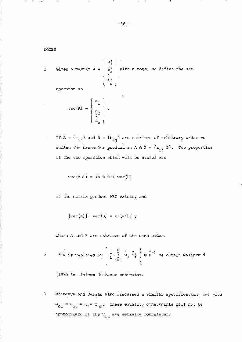
NOTES

1 Given a matrix A

operator as

a'n

with n rows, we define the vec

vec(A)

If A = {a,.} and B = {b. ,} are matrices of arbitrary order we~J ~J

define the Kronecker product as A ~ B = {a" B}. Two properties~J

of the vec operation which will be useful are

vec(ABC) (A ~ C') vec (B)

if the matrix product ABC exists, and

[vec (A) ]' vec (B) tr(A'B) ,

where A and B are matrices of the same order.

2 If W is replaced by l(.!:. ~

N L v,i=l ~

v' ] ~i

A_lM we obtain Malinvaud

(1970) 's minimum distance estimator.

3 Bhargava and Sargan also discussed a similar speci:Ucation, but with

WOl = w02

= ... = wOT

' These equality constraints will not be

appropriate if the vit are serially correlated.

- 37 -

4 The implications of this procedure Were studied by Kie;eer (1980)

in the context of a 'fixed effects' treatment of a static

model.

- 38 -

CHAPTER 2

QML ESTIMATION OF DYNAMIC MODELS WITH SERIALLY CORRELATED ERRORS

2.1 Introduction

This Chapter is concerned with the formulation and estimation by

quasi-maximum likelihood (QML) methods of dynamic random effects models

with first-order autoregressive-first-order moving average time-varying

errors.

Quasi-maximumlikelihood estimators are of interest because they

provide a broad framework for the estimation of mOdels under general

constraints. For this reason they have been commonly used when prior

information on covariance matrices is available. They are specially

attractive in our context, i.e. that of a system of (T+l) equations,

T of which are linked by linear constraints and the remaining one -

the prediction equation for YiO - is in reduced form, since the

nuis,ance coefficients in the latter equation can be easily concentrated

out of the likelihood function (what in fact is an application of the

LIML technique for a subset of equations in a simultaneous system), thus

leading to a criterion function that only depends on the parameters of

interest and where we can still introduce constraints in the covariance

coefficients. However, since normality is not assumed, we cannot rely

upon maximum likelihood asymptotic theory in discussing the properties

of these estimators.

- 39 -

This discussion will be the purpose of Chapter 3. Section 2.2 in

this Chapter introduces the models arising from three different

assumptions about the covariancesbetween the errors in the equation for

YiO and the remaining disturbances in the model. Section 2.3 derives

the concentrated likelihood functions for these three alternative models.

Section 2.4 considers QML estimation with arbitrary intertemporal co-

variance and other alternative asymptotically equivalent methods.

In Section 2.5, the performance of QML methods is investigated, either

for correct models or under several misspecifications - though always

using normal variates - by resorting to experimental evidence. Finally,

Section 2.6 discusses an extended model with arbitrary heteroscedasticity

over time.

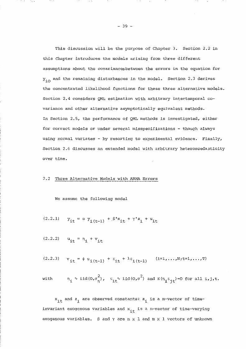
2.2 Three Alternative Models with ARMA Errors

We assume the following model

(2.2.1)

(2.2.2)

a y, ( 1) + B'x't + y'z, + U'tl t- . l l l

n, + V'tl l

(2.2.3) (i=l, ... ,Nit=l, ... ,T)

with

X't and z, are observed constantst z, is a m-vector of time-l l l

invariant exogenous variables and xit

is a n-vector of time-varying

exogenous variables. Band y are n x 1 and m x 1 vectors of unknown

- 40 -

parameters, respectively, and a is an unknown scalar parameter. We

also observe t=O, so that (T+l) time series observations are available

on N cross-sectional units. It is also assumed that I~I < 1 and IAI < 1

so that the error process is stationary and invertible.

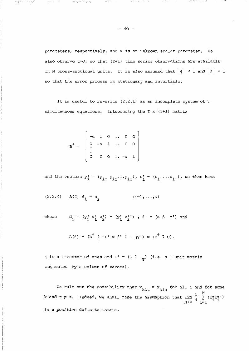
It is useful to re-write (2.2.1) as an incomplete system of T

simultaneous equations. Introducing the T x (T+l) matrix

-a 1 0

o -a 1

o 0

o 0

o 0 0 .. -a 1

and the vectors y~J.

(2.2.4) A(o) d.J.

u,J.

(i=l, ••. ,N)

where d'i

(y ~ x' z ~) = (y ~ z:,') , 0'J. i J. J. J. (a 13' y') and

A (0) -I* ~ 13' - ty') c) •

1 is a T-vector of ones and I* = (0

augmented by a column of zeroes).

IT) (1. e. a T-unit matrix

We rule out the possibility that xk

' = xk

' for all iJ.t J.S

k and t ~ s. Indeed, we shall make the assumption that limN-+oo

is a positive definite matrix.

and for someN

1 'i'- L (z:,z:,')N i=l J. J.

- 41 -

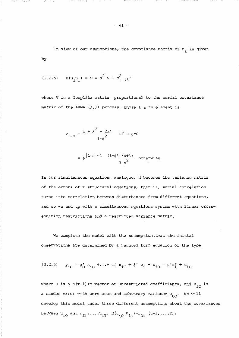
In view of our assumptions, the covariance matrix of u, is given~

by

(2.2.5) E(u,u~)~ ~

2 2~ = 0 V + 0 11'n

where V is a Toeplitz matrix proportional to the serial covariance

matrix of the ARMA (1,1) process, whose t,s th element is

vt

_s if t-s=O

It-sl-lep

(l+ep;\') (ep+;\,)

l_ep2otherwise

In our simultaneous equations analogue, ~ becomes the variance matrix

of the errors of T structural equations, that is, serial correlation

turns into correlation between disturbances from different equations,

and so we end up with a simultaneous equations system with linear cross-

equation restrictions and a restricted variance matrix.

We complete the model with the assumption that the initial

observations are determined by a reduced form equation of the type

(2.2.6) 11 ' z*. + U~ iO

where 11 is a n(T+l)+m vector of unrestricted coefficients, and uiC

is

a random error with zero mean and arbitrary variance woo. We will

develop this model under three different assumptions about the covariances

between u'O and uil, ••• ,u'T' E(u U't)=w (t=l, .•. ,T):~ ~ iO ~ Ot

- 42 -

(i) wOl =•.. = WOT = o. Thus YiO can be regarded as an exogenous

variable in the simultaneous system and so (2.2.4) becomes a

complete model. This is equivalent to the assumption that the

YiO (i=l, .•. ,N) are fixed and known constants.

(ii) Further assuming lal < 1 we may restrict wOl"",wQT on the lines

suggested by Bhargava and Sargan (1983) for models with white

noise errors. In this case we take u. to be1.0

(2.2.7)n.

.,. +_1._+Si l-a

00

Lk=O

ka vi (-k)

where Z;. is a prediction error defined as1.

(2.2.8) Z;.1.

00

L ak

(S'x1.' (-k) + y'z.) - ~'z~k=O 1. 1.

2which is assumed to have constant variance aZ; for all i. So we have

(2.2.9)

with

(2.2.10) 02

2a__n__ + ~t-l ° 2l-a 2 a

(l+~A) (~+A)

(l-a~) (1-~2) ,

(t=l, •.. ,T)

in particular if vit

follows purely a moving average scheme, ~=O and

202 = A, and then, except wOl ' all covariances are equal to an/Cl-a).

2woo is still unrestricted but it can be expressed in terms of aZ; as

follows

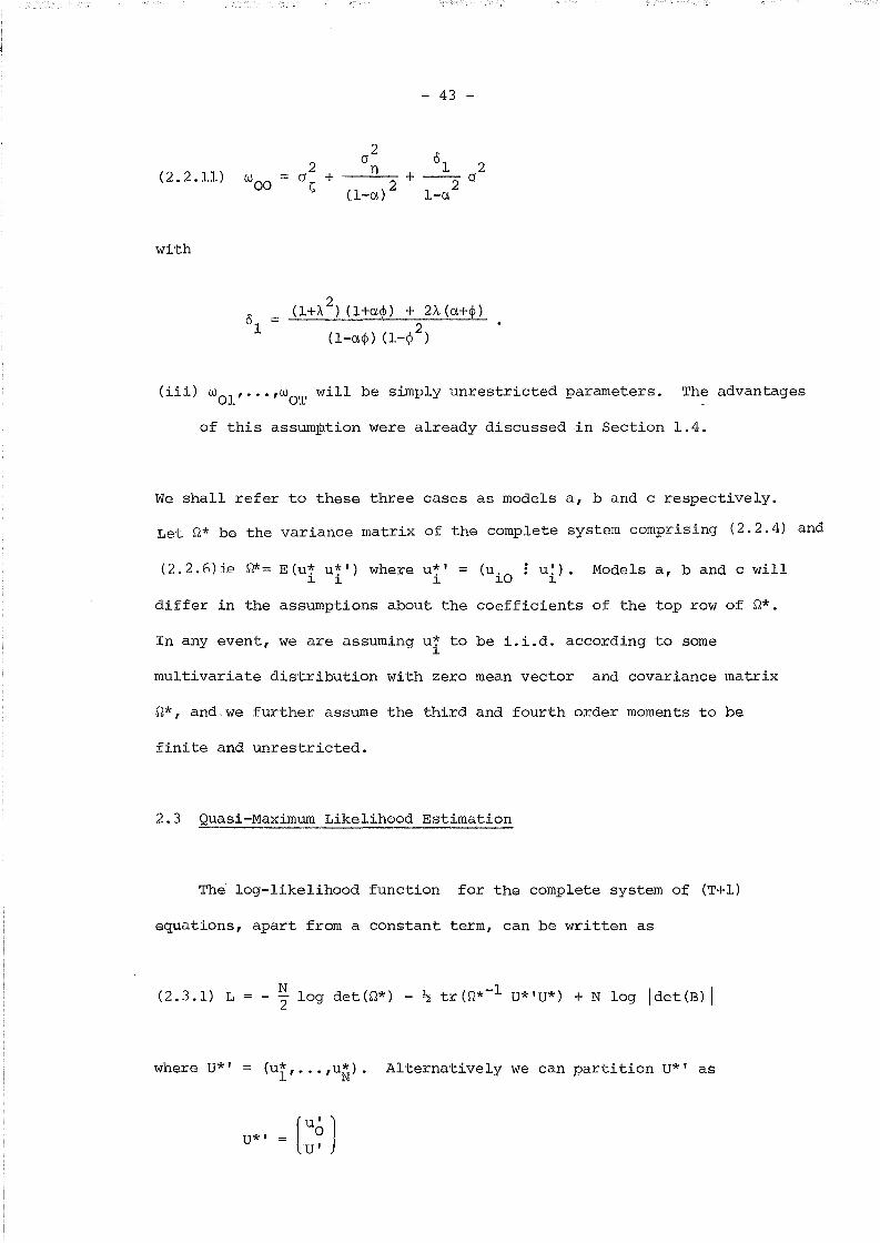
(2.2.11)

with

2(J

n2

(l-a)

- 43 -

(\ 2+ --·-2 (J

l-a

(iii) wOl, ..• ,wOT

will be simply unrestricted parameters. The advantages

of this assumption were already discussed in Section 1.4.

We shall refer to these three cases as models a, band c respectively.

Let ~* be the variance matrix of the complete system comprising (2.2.4) and

(2.2.6)ie ~~ E(u~ u~') where u*' ~ (u.O

: u~). Models a, band c will1 1 i 1 1

differ in the assumptions about the coefficients of the top row of ~*.

In any event, we are assuming u~ to be i.i.d. according to some1

multivariate distribution with zero mean vector and covariance matrix

~*, and we further assume the third and fourth order moments to be

finite and unrestricted.

2.3 Quasi-Maximum Likelihood Estimation

The log-likelihood function for the complete system of (T+l)

equations, apart from a constant term, can be written as

(2.3.1) LN2' log det W*) ~ tr(~*-l U*'U*) + N log \det(B) I

where U*' ~ (ui, •.. ,uN). Alternatively we can partition U*' as

U*' ~ (:? J

- 44 -

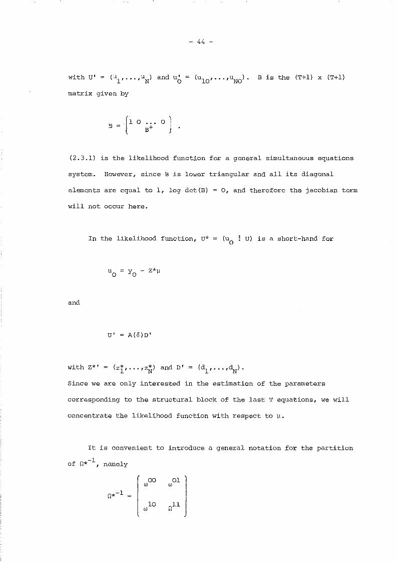
matrix given by

(U lO , .•. ,uNO). B is the (T+l) x (T+l)

Bo '\

J

(2.3.1) is the likelihood function for a general simultaneous equations

system. However, since B is lower triangular and all its diagonal

elements are equal to 1, log det(B) = 0, and therefore the jacobian term

will not occur here.

In the likelihood function, U*

and

U' A(o)D'

U) is a short-hand for

Since we are only interested in the estimation of the parameters

corresponding to the structural block of the last T equations, we will

concentrate the likelihood function with respect to ~.

It is convenient to introduce a general notation for the partition

of rt*-l, namely

00 01tU tU

- 45 -

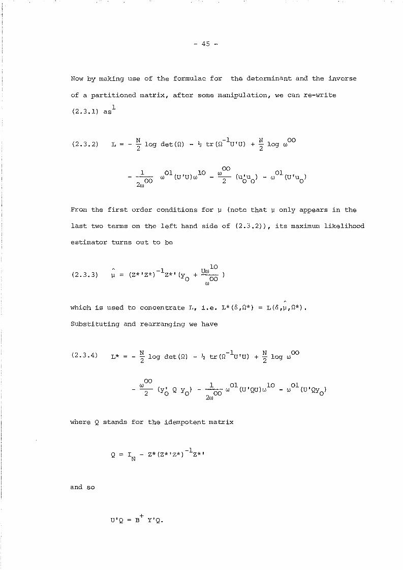
NoW by making use of the formulae for the determinant and the inverse

of a partitioned matrix, after some manipulation, we can re-write

1(2.3.1) as

(2.3.2)N

L = - 2 log det(~) --1 N 00

~ tr(~ U'U) + 2 log w

00wOl(U'U)wlO _ w

201

(u'u ) - w (U'uO

)o 0

From the first order conditions for ~ (note that ~ only appears in the

last two terms on the left hand side of (2.3.2)), its maximum likelihood

estimator turns out to be

(2.3.3)-1(z* , z*) z*' (y

ouw lO

+-­00

w

which is used to concentrate L, i.e. L*(8,~*)

Substituting and rearranging we have

L (8,~,~*) •

(2.3.4) L* = N2 log det (Q) --1 N 00

~ tr(~ U'U) + 2 log w

00w

21 01 10

(y ' Q y) -- w (U'QU)wO 0 - 00

2w

where Q stands for the idempotent matrix

and so

Q

U'Q

I - z*(z*'z*)-lz*'N

+B Y'Q.

01W = 0

- 46 -

In what follows we specialise the likelihood function (2.3.4) to the

models a, band c introduced in the previous section.

Model a

00In model a, ~Ol = (W01, ••. ,WOT ) = (0, .•. ,0) so that W = l/Woo '

and Qll = Q-l. Enforcing these restrictions in (2.3.4) we

obtain

(2.3.5) N- "2 log det(Q) -

Since the last two terms are irrelevant in so far as the maximisation

with respect to 0 and the constraint parameters in Q is concerned,

we may just consider maximising

(2.3.6) L aN -1- "2 log det(Q) - ~ tr(Q UIU)

This is the kind of likelihood function that was considered by

Balestra and Nerlove (1966).-1Note that tr(Q UIU) =

-1(vec (D)] I (IN e S""l ) vec (U), and using the stacked regression notation

introduced in Chapter 1 we have

(2.3.7)-1 + -1 +

trW DIU) = (y - X O)'(IN

e Q )(y - X 0)

Here, we follow Bhargava and Sargan (1983) in parameterising Q as

(2.3.8) (J2

(V + p2

\ 1 I )

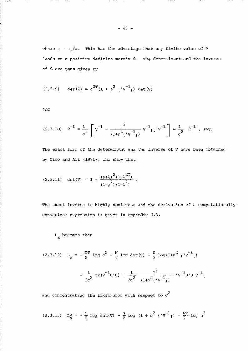
- 47 -

where p. = a la. This has the advantage that any finite value of Pn

leads to a positive definite matrix~. The determinant and the inverse

of ~ are thus given by

(2.3.9)

and

det(Q)

(2.3.10)-1

~1

2a

--1~ , say.

The exact form of the determinant and the inverse of V have been obtained

by Tiao and Ali (1971), who show that

(2.3.11) det(V)

The exact inverse is highly nonlinear and the derivation of a computationally

convenient expression is given in Appendix 2.A.

L becomes thena

(2.3.12) La

NT 2 N N 2-12 log a - 2" log det(V) - 2" log(HP 1 IV 1)

2P

2 -1(Hp 1 IV 1)

-1 -11 IV UIU V 1

2and concentrating the likelihood with respect to a

(2.3.13) L*a

N N 2 -1 NT 2- 2" log det(V) - 2" log (1 + P 1 IV 1) - ~ log s

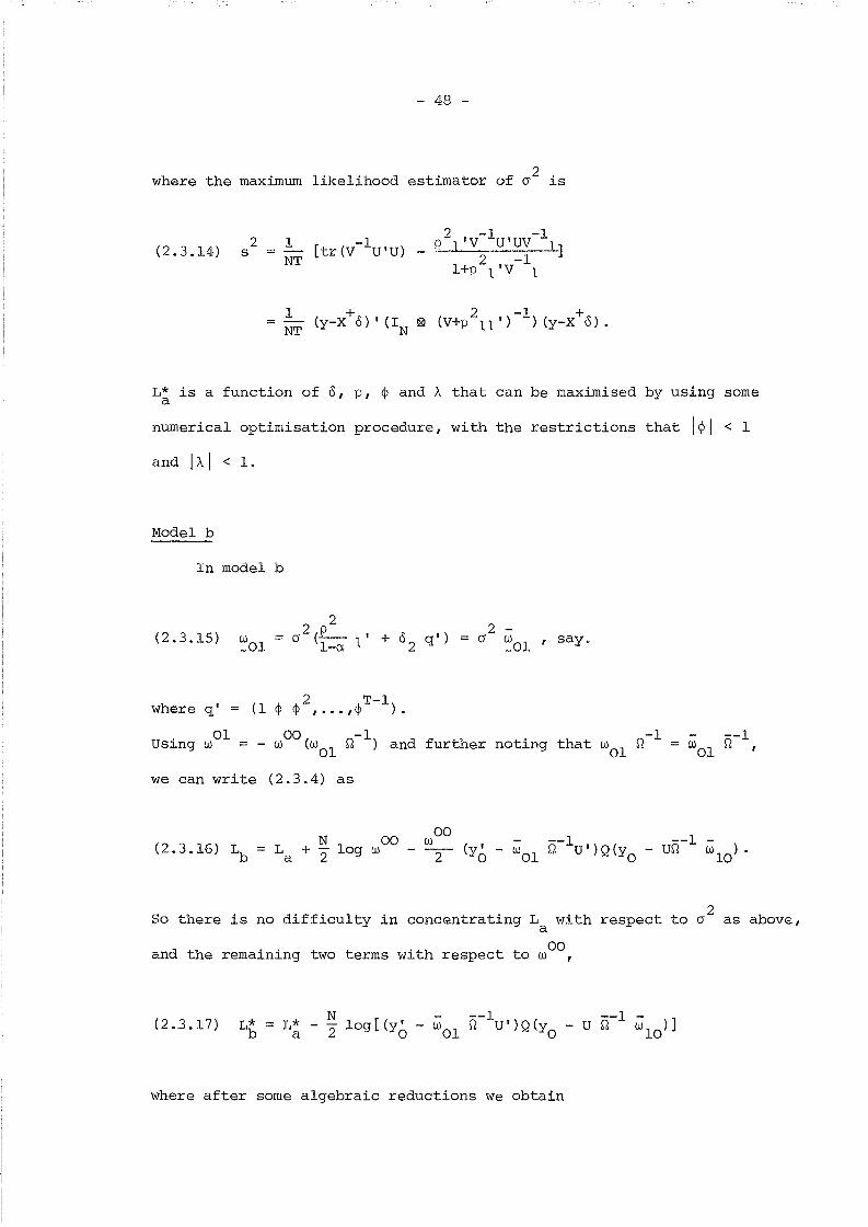
- 48 -

2where the maximum likelihood estimator of cr is

(2.3.14)2

s2 -1 -1

1 -1 P 1 'V U'UV 1NT [tr(V U'U) - 2 -1 ]

l+p 1 'V 1

1 + 2 -1 +NT (y-X 0)' (IN ~ (V+p 11') ) (y-X 0).

L* is a function of 8, p, ~ and A that can be maximised by using somea

numerical optimisation procedure, with the restrictions that I~I < 1

and IAI < 1.

Model b

In model b

(2.3.15) ~Ol

2cr 2 (_p__ l' + °

2q')

I-a2 -

cr ~Ol' say.

2 T-lwhere q' = (1 ~ ~ , •.. ,~ ).

Using wOl = - WOO(WOl

Q-l) and further noting that wOl

Q-l

we can write (2.3.4) as

--1= (001 n ,

2So there is no difficulty in concentrating L with respect to cr as above,

a

and the remaining two terms with respect to wOO,

(2.3.17) L*b

L*a

N- log[ (y'2 °

where after some algebraic reductions We obtain

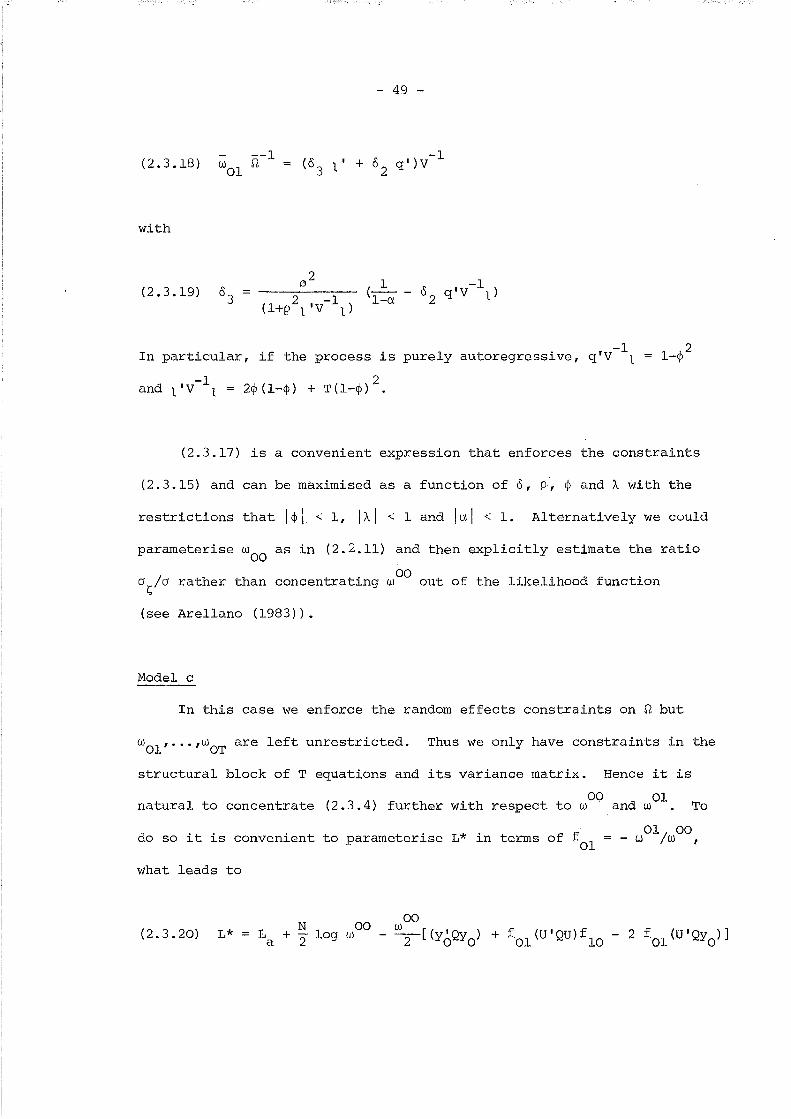
(2.3.18 )

with

- 49 -

-1(01'+0 q')V

3 2

(2.3.19) 03

. 1 ., -1 1-"2In particular, if the process ~s pure y autoregress~ve, q V 1 ~

-1 2and l' V 1 = 2~ (l-~) + T (1-~ ) •

(2.3.17) is a convenient expression that enforces the constraints

(2.3.15) and can be maximised as a function of 0, P, ~ and A with the

restrictions that I~I < 1, 1\1 < 1 and lal < 1. Alternatively we cuulu

parameterise wOO as in (2.2.11) and then explicitly estimate the ratio

00as/a rather than concentrating w out of the likelihood function

(see Arellano (1983)).

Model c

In this case we enforce the random effects constraints on ~ but

W01, ... ,WOT

are left unrestricted. Thus we only have constraints in the

structural block of T equations and its variance matrix. Hence it is

00 01natural to concentrate (2.3.4) further with respect to wand W • To

. 01 00do so it is convenient to parameterise L* ~n terms of f

Ol= - W /w ,

what leads to

(2.3.20) L*N 00

La + 2 log w00T[(Y~QYo) + f

Ol(U'QU)f

lO- 2 f 01 CU'QYo )]

- 50 -

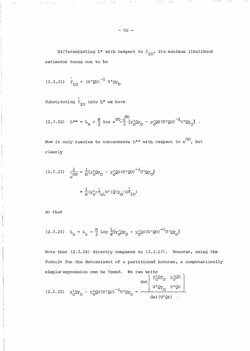
Differentiating L* with respect to f lO ' its maximum likelihood

estimator turns out to be

(2.3.21) 1=~10

-1(U'QU) U'QYO

A

Substituting flO

into L* we have

(2.3.22) L**

00Now it only remains to concentrate L** with respect to w but

clearly

(2.3.23) A~O = ~[YoQYo - YoQU(U'QU)-lU'QYo]w

so that

(2.3.24) Lc

La ~ log ~[YoQYo

Note that (2.3.24) directly compares to (2.3.17). However, using the

formula for the determinant of a partitioned inverse, a computationally

simpler expression can be found. We can writeYo'Qyo y'QU

det 0

(2.3.25)-1

y'Qy - y'QU(U'QU) U'Qy000 0

U'Qy U'QUo

det (U'QU)

- 51 -

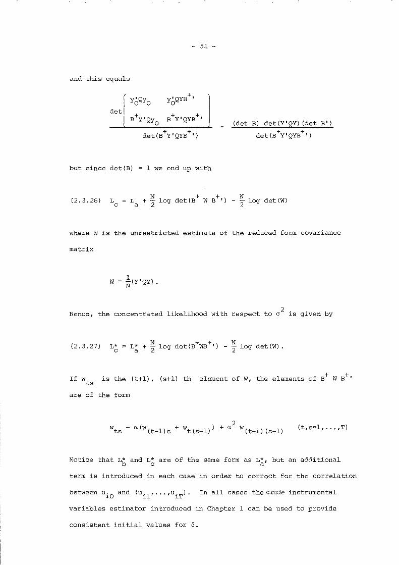
and this equals

rdetl

I+ +det(B Y'QYB ')

(det B) det(Y'QY) (det B')

det (B+Y'QYB+')

but since det(B) 1 we end up with

(2.3.26) Lc

N + + NLa + 2 log det(B W B ') - 2 log det(W)

where W is the unrestricted estimate of the reduced form covariance

matrix

W ~(Y'QY) .

2Hence, the concentrated likelihood with respect to a is given by

(2.3.27) L*c

If w is the (t+l), (s+l) th element of W, the elements of B+ W B+'ts

are of the form

2wts - et (w (t-l) s + wt (s-l)) + et 'iN (t-l) (s-l) (t, s=1, ••. , T)

Notice that Lb and L~ are of the same form as L~, but an additional

term is introduced in each case in order to correct for the correlation

between u iO and (uil' ... ,uiT). In all cases thec~de instrumental

variables estimator introduced in Chapter 1 can be used to provide

consistent initial values for o.

- 52 -

2.4 Estimation with Arbitrary Intertemporal Covariance

We can define the QML estimator of 0 that treats ~* as an

arbitrary symmetric positive definite matrix. Since (2.3.26) has

already been concentrated with respect to V, wOO' wOl, ... ,wOT ' the relevant

likelihood here can be obtained simply by concentrating (2.3.26) further

with respect to ~, where L is now as given in (2.3.6). The maximuma

likelihood estimation of ~ is

(2.4.1) .!.. U'UN

N

~A(O)( Ii=l

d.d~)A' (0)1. 1.

so that we obtain a likelihood function which only depends on 0 (cf.

Bhargava and Sargan (1983)) given by

(2.4.2) N log det(U'U) + N log det(B+WB+') - ~ log det(w)2 N 2 2

Since the covariance matrix is unrestricted, this is an application

of the limited information (quasi) maximum likelihood (LIML) method

to a subset of equations, and its asymptotic properties are well known

in the literature.2

In particular, it is asymptotically equivalent to

the three stage least squares (3SLS) estimator applied to that subset

of equations (e.g. see Sargan (1964)). The advantage of the latter

is that, since the restrictions in A(O) are linear, it is the solution

of a set of linear equations and therefore it can be calculated without

requiring iterative optimization techniques. However, we are still

interested in the QML estimator as it will allow us to discuss (quasi)

likelihood ratio tests of covariance restrictions at a later stage and,

more generally, its relation to the QML procedures discussed in Section 2.3.

- 53 -

In any event, the 3SLS estimator of °minimises

(2.4.3)-1 ~-l

[vec (D)] , (Z* (Z* I Z*) Z* I ® rI ) vec (D)

where rI is a consistent estimator of ri, e.g. rIA N A

(l/N)A(o ) (L. ld.d~)A' (oCI )CIV ~= ~ ~ V

and 0CIV is the crude instrumental variables estimator of ° introduced

in Section 1.3. Again, using vec(D) = y-x+o, the explicit solution

of (2.4.3) is given by

(2.4.4)

However, (2.4.4) is not an useful expression from a computational

point of view. The reason is that since N is large and T is small,

it is convenient to compute the second order moments datq matrix

(l/N)\~ l(d.d~) just once and construct from it the relevant statistics,L~= 1. ~

thus avoiding the storage of arrays of dimension N, or having to perform

successive summations of N products. First, notice that

+ +where X

tis the N x (l+n+m) matrix X

t= (Yt-l X

tZ) and d

tis aT-vector

with one in the th position and zero elsewhere. Equally

so that

- 54 -

T;-1) [

T[ I (x+' d')] (z* (z*' z*) -lz* I I (x

+~ d )]~ ~

t=l t t s=l s s

Letting~-l {:ts}, and since d'

~-l

d~ts

Q = Q w we havet s

T T~ts A+, A+ -1 T T _

A+,(2.4.5)

°3SLS( L I w X

tx ) I I w

ts Xt Ys

t=l s=ls

t=l s=l

where

(2.4.6)

and

Z*(Z*'Z*)-l(Z*'y )t

(t=O , 1, •.. ,T)

Moreover using the fact that d~ d s = 0 for t f sand dt dt

= 1, the

corresponding expression for the crude instrumental variables

estimator is

(2.4.7)T

( It=l

Finally, we make some remarks on identification issues. The basic

identification condition is that lilUN-+=(l/N) (Z*'Z*) should be positive

definite; if further T > 1 and at least some element of the vector ~O

is non-zero, the mOdel with unrestricted covariance matrix is identified.

Alternatively, if we are not willing to state conditions in terms of

- 55 -

~o' the requirements are that at least some element of S is non-zero

and T > 2. Therefore, a necessary condition for identification is

that n > 1. Turning to restricted models,if T=l, Q* has three

different elements so that a random effects specification with white

noise time-varying errors of type b is just identified. Identification

of ARMA(l,l) models requires that T > 3.

2.5 Experimental Evidence

Given the existence in the literature of a certain amount of

conflicting Monte-Carlo results on the performance of v~rious maximum­

likelihood methods for dynamic random effects models, (cf. Nerlove (1971),

Maddala (1971), Bhargava and Sargan (1983)) it was decided to carry

out some simulation experiments in order to investigate the practical

performance of the methods introduced in this Chapter. We are

particularly interested in the consequences of incorrectly specifying

yO as exogenous when the errors are serially correlated. We also wish

to obtain some insight into how the methods that do not constrain Q*

compare to those in which the covariance restrictions are enforced,

and how models band c compare in turn. Finally, it is important to

inspect the ability of these procedures in distinguishing among different

serial correlation schemes and between dynamics (lagged endogenous

variables) and serial correlation.

Five different sets of samples were generated from models of the

form

- 56 -

E:i (t-l)

(i 1, ... ,100 t 1, ••• , 20)

where ni

~ NID(O, .16), E:it

~ NID(O, .25)

YiO

= viO

= o.

2(Le . .p .64), and

The exogenous

previous studies

variables were generated in a similar way as in

where P't ~ NID(O,l) and r. ~ NID(O,l). The first ten cross-sectionsl l

were discarded so that YO is an endogenous variable in the system

and the same process for v, has been holding in the past.It

We are thus left with T = 9 and N = 100.

The five sets of data correspond to the following values of

a, </> and A:

- 57 -

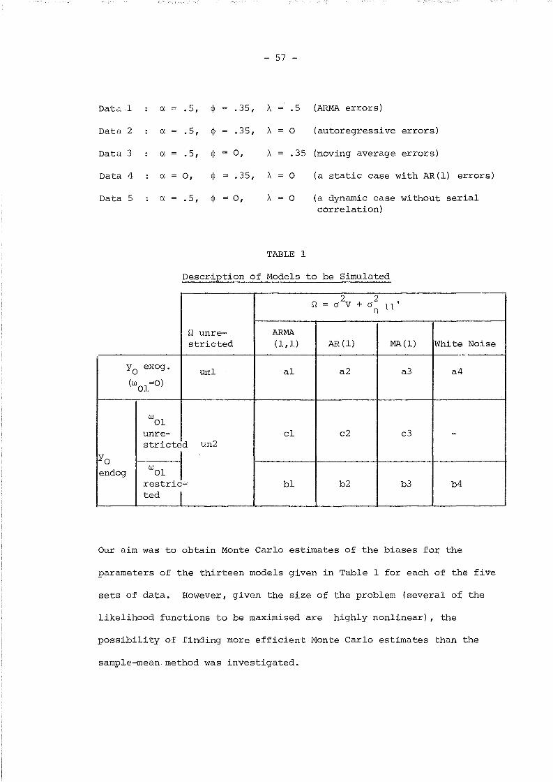
Data 1 a = .5, </> .35, A .5 (ARMA errors)

Data 2 a = .5, </> .35, A- 0 (autoregressive errors)

Data 3 a = .5, </> 0, A- .35 (moving average errors)

Data 4 a = 0, </> .35, A- 0 (a static case with AR(l) errors)

Data 5 a = .5, </> 0, A- 0 (a dynamic case without serialcorrelation)

TABLE 1

Description of Models to be Simulated

Q2 2

11 '= (J V + (J

n

Q unre- ARMAstricted (1,1) AR(l) MA(l) White Noise

yo exog. unl al a2 a3 a4(W

Ol=0)

W01

unre- cl c2 c3 -stricted un2

yo

~endogrestric..;... bl b2 b3 b4ted I

Our aim was to obtain Monte Carlo estimates of the biases for the

parameters of the thirteen models given in Table 1 for each of the five

sets of data. However, given the size of the problem (several of the

likelihood functions to be maximised are highly nonlinear), the

possibility of finding more efficient Monte Carlo estimates than the

sample-mean method was investigated.

- 58 -

If the bias is denoted by 8=E(o - 0), its standard Monte-Carlo

A H A

estimate based on H replications is given by 8 = (l/H) Lj=l (OJ-o), where

O. is the estimate of 8 obtained in the jth replication, and e isJ

unbiased for 8. 8. depends on a particular set of (0,1) normalJ

variates obtained from some pseudo-random numbers generator, i.e.

0,.= o(u,). In the antithetic variate technique a second unbiasedJ:: J

estimator 8* is sought, having negative correlation with 8. Then

6 = ~(8 + 8*) will also be an unbiased estimator of 8 with variance

Var(6) = ~ Var(8) + ~ Var(8*) + ~ Cov(8,8*). If 8* is a sample

mean that has been constructed from a further set of random

replications, then Cov(8,8*) = o. However, since u. are standardJ

normal variates so are -u. and, clearly, an estimator 8* of theJ

form

H8* 1 L (8 (-u ,) - 0)

H j=l J

will also be an unbiased estimator of 8. Now since u. and -u, areJ J

perfectly negatively correlated, it can be the case that a negative

covariance is induced between 8 and 8*, so that 8 would have a smaller

variance than the sample mean estimator based on an equal number of

replications (cf. Hammersley and Handscomb (1964) and Hendry (1984)).

In previous studies it has been noticed the difficulty of finding

antithetic transformations which reduce the variance of Monte Carlo

estimators for dynamic models (cf. Hendry and Harrison (1974)).

However, the simultaneous equationsanal09ue provides a different

perspective in the case of models from panel data and in this context

it seemed worth to re-use the random numbers in pairs of opposite sign.

- 59 -

The situation can be illustrated by mean of a simple example.

If we take T = 1, n = 1 and m = 0, our general model becomes

(i=l, ••. ,N)

This model is exactly identified so that the QML estimator of

0' = (a S) that leaves ~* unrestricted is identical to the 2SLS

estimator, and it equals

-1(X'W) X'y

1

with X (Yo xl)' After some manipulation we have

1;;' u1a - a

where ~ is the vector of least squares residuals from regressing

constant over the replications, and so is c, that is given by c = ~'X~.

Now, notice that a trial of a-a based on (-uo' -ul ) yields

transformation, a negative covariance is still generated between these

antithetic pairs.

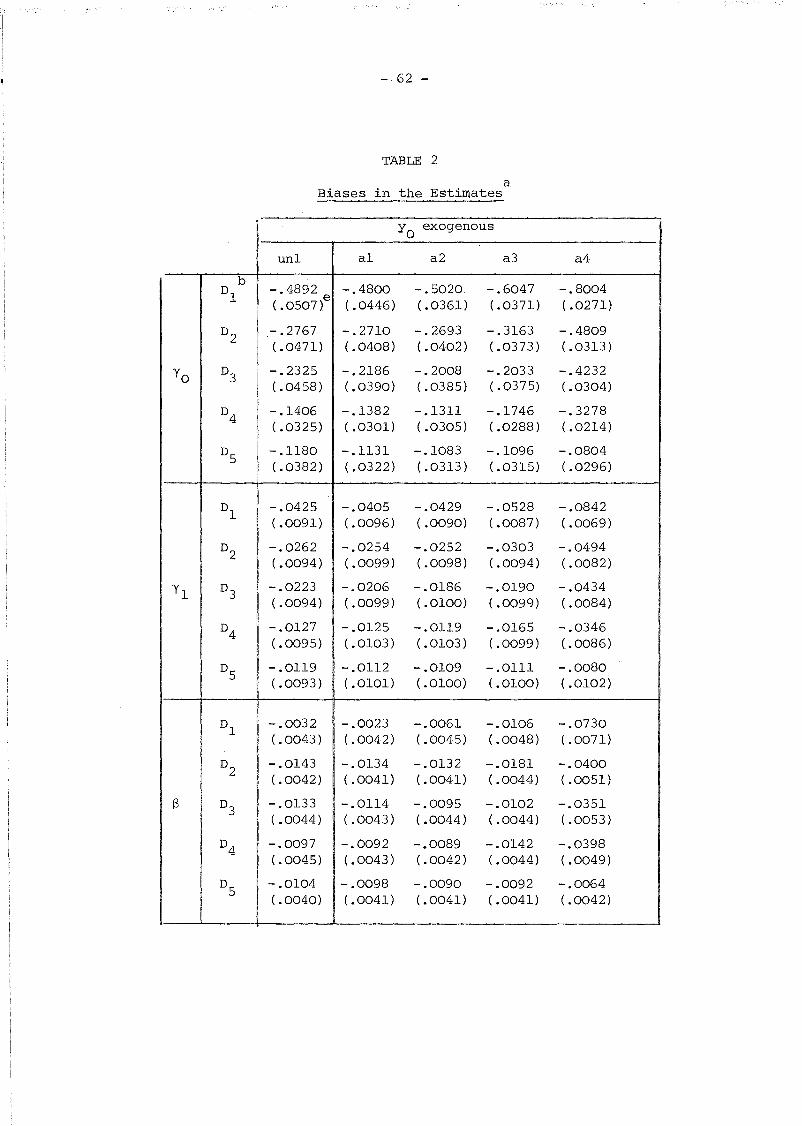
Thus the results reported in Table 2 were obtained from 20

replications corresponding to 10 antithetic pairs (uit ' - uit) , Le.

every trial was performed twice, and the resulting estimates were

- 60 -

averaged. In all cases, the non-deriv~truve Gill-Murray-Pitfield algorithm

E04JBF implemented in the Nag Library, Mark IX was used to optimise

the log-likelihood functions.

First considering the consequences of misspecifying the initial

conditions, Le. wrongly assuming that w01

=- ••• = wOT

= 0, our results

for the set of samples with white noise time-varying errors (data 5)

and models unl and a4 fairly generally agree with those reported by

Bhargava and Sargan (1983). Indeed, these biases are rather small with

the exceptions perhaps of the intercept; for example, the bias of a

is .0396 for model unl and .0263 for model a4. However, as one would

expect, the consequences of treating yo as exogenous are rather more

serious when the vit

are also serially correlated. To take an extreme

case, for the ARMA(l,l) samples (data 1) and model a4 the biases of

a and yoare ten times larger than those obtained with the same model

for data 5, but even if the ARMA(l,l) structure is properly specified

and model al is used, these biases still are between 5 and 6 times

bigger.

The cases where the endogeneity of yo is properly specified (both

for models b and c) and no misspecifications are present in vit ' perform

extremely well and the biases are almost negligible. Turning to the

comparison between model un2 and models band c, the Monte Carlo finite

sample standard deviation of the estimates (which is just I2lJ times the

standard errors of bias) are slightly lower for models band c in the

case of a and yO' and roughly the same for Yl and S; on the other hand,

it does not appear to be any noticeable difference, both in terms of

- 61 -

bias and standard deviation, between models band c. These results

suggest that in the QML framework un2 is a highly convenient method

of estimation at the early stages of model building and that if we are

interested in the structure of Q*,models c, that leave wOl, ..• ,wOT

unrestricted, can achieve similar results to models b at a lower

computational cost.

Data 4 (with a=O and ~=.35) were generated to check the ability

of our simulated model to distinguish systematic dynamics from serial

correlation, and at least in this case, the results turned out to be

extremely satisfactory. No doubt, this ability will depend on the

characteristics of the process generating the time-varying exogenous

variables.

Finally, we remark that models bl and cl (those allowing for

ARMA(l,l) errors) are able to identify the correct serial correlation

scheme in every case and therefore they are useful in order to choose

between purely autoregressive and purely moving average schemes.

2.6 A Model with Arbitrary Heteroscedasticity over Time

If the presence of heteroscedasticity over time in the random

effects model is suspecte~equation (2.2.3) can be extended on the

lines suggested in Section 1.5 by assuming:

(2.6.1)

(2.6.2) ~vi (t-l) + s·it + AS i (t-l) (i=l, •.. ,Ni t=l, •.. ,T)

- 62 -

TABLE 2

aBiases in the Estimates

Yo exogenous

, un1 a1 a2 a3 a4

b-.4892 -.4800 -.5020 -.6047 -.8004D

1 e(.0446) ( .0361) ( .0371) ( .0271)(.0507)

D2

-.2767 -.2710 -.2693 -.3163 -.4809( .0471) ( .0408) ( .0402) ( .0373) (.0313)

YOD

3-.2325 -.2186 -.2008 -.2033 -.4232(.0458) (.0390) ( .0385) ( .0375) ( .0304)

D4

-.1406 - .1382 -.1311 -.1746 -.3278( .0325) ( .0301) ( .0305) ( .0288) ( .0214)

D5

- .1180 -.1131 -.1083 -.1096 -.0804( .0382) ( .0322) (.0313) ( .0315) ( .0296)

D1

j-.0425 -.0405 -.0429 -.0528 -.0842( .0091) ( .0096) ( .0090) ( .0087) ( .0069)

D2

-.0262 -.0254 -.0252 -.0303 -.0494( .0094) ( .0099) ( .0098) ( .0094) ( .0082)

Y1D

3-.0223 -.0206 -.0186 -.Ol90 -.0434( .0094) ( .0099) ( .0100) ( .0099) ( .0084)

D4

-.0127 -.0125 -.0119 -.0165 -.0346(.0095) (.0103) ( .0103) ( .0099) (.0086)

D5

-.0119 - .0112 -.0109 -.0111 -.0080(.0093) ( .0101) ( .0100) ( .0100) ( .0102)

D1

-.0032 -.0023 -.0061 -.0106 -.0730( .0043) (.0042) ( .0045) ( .0048) (.0071)

D2

-.0143 -.0134 - .0132 -.0181 -.0400(.0042) ( .0041) ( .0041) (.0044) ( .0051)

(3 D3

-.0133 -.0114 -.0095 -.0102 -.0351( .0044) (.0043) ( .0044) ( .0044) (.0053)

D4

-.0097 -.0092 -.0089 -.0142 -.0398( .0045) (.0043) ( .0042) ( .0044) ( .0049)

D5

-.0104 -.0098 -.0090 -.0092 -.0064( .0040) (.0041) (.0041) ( .0041) ( .0042)

TABLE 2 continued

- 63 -

y exogenous0

unl al a2 a3 a4

D1

.1319 .1283 .1370 .1676 .2677( .01l0) (.0095) ( .0075) ( .0079) ( .0068)

D2

.0846 .0820 .0814 .0976 .1580( .0106) ( .0088) ( .0087) ( .0080) ( .0072)

Cl'. D3 .0722 .0667 .0605 .0617 .1390

(.0102) ( .0082) ( .0080) ( .0077) ( .0069)

D4 .0861 .0840 .0800 .1l00 .2263

( .0123) ( .01l1) ( .01l1) ( .0105) ( .0064)

D5

.0396 .037-6 .0358 .0362 .0263( .0081) (.0066) ( .0063) ( .0064) ( .0057)

,

D1 -.3397 -.5633 -.3509 -.5044

(.0335) ( .0207) (.0294) ( .0134)

D2 - .1858 -.1874 -.1958 -.3091

(.0295) ( .0296) ( .0286) ( .0218)

p D3 -.1600 -.1872 -.1558 -.3056

( .0302) (.0283 ) (.0296) (.0213)

D4 -.0761 -.0520 -.0574 -.1954

( .0253) ( .0245) (.0242) ( .0159)

D5 -.0596 -.0702 -.0707 -.0532

( .0239) ( .0260) ( .0261) ( .0246)

D1 -.1123 .2491

( .0105) (.0056)

D2 -.1054 -.0725

( .0203) ( .0068)

cl> D3 -.0809 d

( .0191)

D4 .0159 -.0859

( .0205) ( .01l4)

D5 c -.0317

( .0060)

D1 .0079 .1460

( .0072) ( .0052)

D2 .0324 d

( .0163)

A- D3 .0275 -.0423

(.0159) ( .0048)

D4 -.1021 d

(.0221)

D5 c -.0332

( .0065)

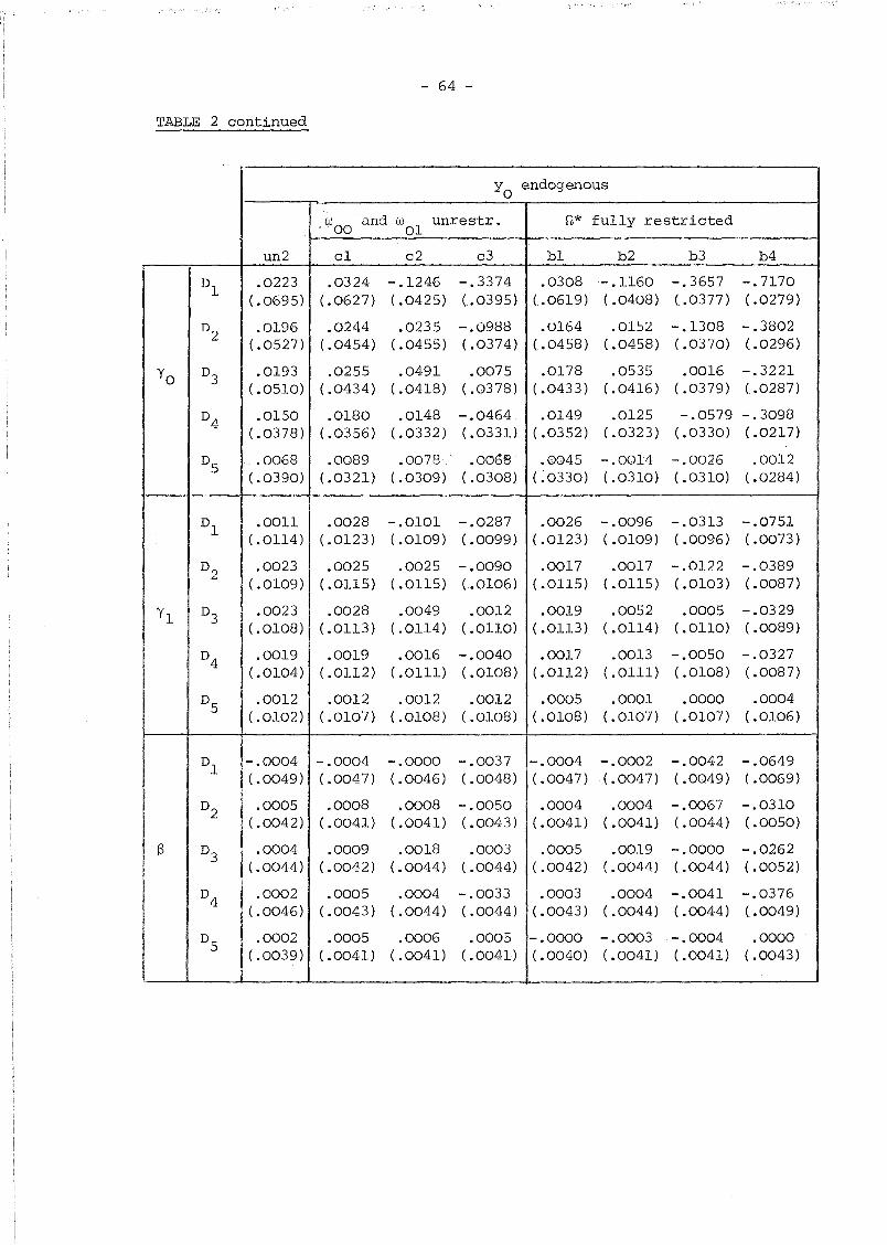
TABLE 2 continued

- 64 -

YOendogenous

w and w unrestr. $1* fully restricted00 01

un2 cl c2 c3 bl b2 b3 b4,D

l.0223 .0324 -.1246 -.3374 .0308 -.1160 -.3657 -.7170

( .0695) ( .0627) ( .0425) (. .0395) (.0619) ( .0408) (.0377) ( .0279)

D2

.0196 .0244 .0235 -.0988 .0164 .0152 -.1308 -.3802( .0527) (.0454) ( .0455) ( .0374) ( .0458) ( .0458) ( .0370) (.0296)

Yo D3

.0193 .0255 .0491 .0075 .0178 .0535 .0016 -.3221(.0510) ( .0434) ( .0418) (.0378) (.0433) (.0416) (.0379) (.0287)

D4

.0150 .0180 .0148 -.0464 .0149 .0125 -.0579 -.3098(.0378) (.0356) (.0332) (.0331) (.0352) (.0323) (.0330) ( .0217)

D5

.0068 .0089 .0078, .0ObB' .0045 -.0014 -.0026 .0012( .0390) ( .0321) ( .0309) ( .0308) ( .0330) ( .0310) ( .0310) ( .0284)

D1

.0011 .0028 -.0101 -.0287 .0026 -.0096 -.0313 -.0751( .0114) (.0123) ( .0109) ( .0099) ( .0123) ( .0109) ( .0096) (.0073)

D') .0023 .0025 .0025 -.0090 .0017 .0017 -.O1/.2 -.0389'" ( .0109) ( .0115) ( .0115) ( .0106) ( .0115) ( .01l5) ( .0103) ( .0087)

YlD

3.0023 .0028 .0049 .0012 .0019 .0052 .0005 -.0329

(.0108) ( .0113) (.0114) (.01l0) ( .01l3) ( .01l4) (.01l0) ( .0089)

D4

.0019 .0019 .0016 -.0040 .0017 .0013 -.0050 -.0327(.0104) ( .01l2) ( .01ll) ( .0108) ( .01l2) (.Olll) ( .0108) ( .0087)

D5

.0012 .0012 .0012 .0012 .0005 .0001 .0000 .0004( .0102) ( .0107) ( .0108) ( .0108) (.0108) (.0107) (.0107) ( .0106)

Dl

-.0004 -.0004 -.0000 -.0037 -.0004 -.0002 -.0042 -.0649( .0049) ( .0047) ( .0046) ( .0048) (.0047) ( .0047) ( .0(49) ( .0069)

D2

.0005 .0008 .0008 -.0050 .0004 .0004 -.0067 -.0310( .0042) ( .0041) ( .0041) ( .0043) ( .0041) ( .0041) ( .0044) ( .0050)

13 D3

.0004 .0009 .0018 .0003 .0005 .0019 -.0000 -.0262( .0044) ( .0042) ( .0044) ( .0044) ( .0042) ( .0044) ( .0044) ( .0052)

D4

.0002 .0005 .0004 -.0033 .0003 .0004 -.0041 -.0376( .0046) ( .0043) (.0044) ( .0044) ( .0043) ( .0044) ( .0044) (. .0049)

D5

.0002 .0005 .0006 .0005 -.0000 -.0003 -.0004 .0000( .0039) ( .0041) ( .0041) ( .0041) ( .0040) ( .0041) (.0041) ( .0043)

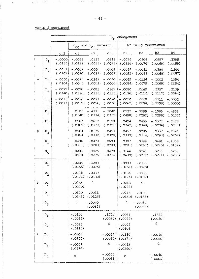
TABLE 2 continued

- 65 -

Yo endogenous

WOO and w01

unrestr. Q* fully restricted

un2 cl c2 c3 bl b2 b3 b4

D1

-.0050 -.0079 .0329 .0919 -.0074 .0309 .0997 .2395( .0144) (.0129) ( .0083) (.0073 ) (.0126) ( .0076) ( .0069) (.0059)

D2

-.0051 -.0069 -.0066 .0301 -.0044 -.0041 .0399 .1244( .0109) ( .0090) ( .0091) ( .0069) (.0091) ( .0092) ( .0069) ( .0057)

a DJ -.0050 - .0073 -.0112 -.oo?-O -.0049 -.OEi4 -.0002 .1054( .0104) ( .0085) ( .0081) ( .0068) (.0084) ( .0079) (.0069) (.0054)

D4

-.0079 -.0098 -.0081 .0287 -.0080 -.0069 .0357 .2139(.0140) (.0128) (.01l5) (.01l5) (.0126) ( .01l0) (.0117) ( .0064)

D5

-.0015 -.0026 -.0023 -.0020 -.0010 .0008 .001l -.0002( .0077) ( .0059) (.0056) ( .0056) ( .0062) ( .0056) (.0056) (.0050)

D1

.0503 -.4331 -.1040 .0727 -.3095 -.1565 -.4953( .0540) (.0334) (.0357) (.0498) ( .0260) ( .0296) (.0132)

D2

.0567 .0612 .0129 .0424 .0455 - .0377 -.2478(.0365) ( .0373) ( .0321) (.0342) (.0349) ( .0289) (.02ll)

p D3

.0563 .0175 .0453 .0457 .0285 .0337 -.2391(.0363 ) ( .0332) (.0328) ( .0338) ( .0314) (.0298) (.0202)

D4

.0496 .0473 .0693 .0387 .0399 .0491 -.1859(.0311) (.0283) ( .0299) ( .0291) (.0267) (.0270) (.0162)

D5

-.0284 .0425 .0420 -.0144 .0241 .0235 .0253( .0478) (.0275) ( .0274) (.0430) ( .0272) (.0271) (.0253 )

D1

.0204 .3209 .0089 .2935(.0155) ( .0075) ( .0161) ( .0070)

D2

.0138 .0039 .0134 .0036(.0176) ( .0100) ( .0174) ( .0102)

~ D3

.0345 d .0218 d( .0210) ( .0233)

D4

.0120 .0051 .0216 .0109(.0145) ( .0128) ( .0160) (.0133 )

D5

c -.0040 c -.0037( .0065) ( .0066)

D1

-.0103 .1724 .0061 .1722( .0069) (.0052) ( .0062) ( .0050)

D2

-.0093 d -.0097 d

(.01l7) (.0108

A- D3

-.0306 -.0057 -.0189 -.0046( .0155) (.0054) (.0172) (.0050)

D4

-.0041 d -.0085 d

( .0174) (.0190)

D5 c -.0048 c -.0046

(.0064 ) (.0065)

- 66 -

NOTES TO TABLE 2

aN = 100, T 9, 20 replications (10 pairs of antithetic variates) •

b D.1.

Data i.

~ = -:\.

c

d

The ARMA(l,l) process degenerates into a white noise for any

Therefore, if the process generating v. is white noise1.t

(as in DS) ~ and :\ are not identified for models al, bl and cl. For

our 20 replications the results turned out to be the following

Model al Model bl Model cl

Converged to </>=:\=0 11 13 16

Converged to ~=l, :\=-1 J 3 3

Converged to ~=-l, :\=1 1 0 1

Converged to otherantithetic pairs S 4 0

When the true vit's are autoregressive (moving average) and the

estimated model only allows for a moving average (autoregressive)

scheme, the MA (AR) coefficient picks up the effect of the serial

correlation, so that it cannot be regarded as an estimate of its

(zero) true value.

e Standard errors of bias are in parentheses.

- 67 -

with bit ~ iid (0,1). This reduces to the former case if 0t = 0 for

all t and we noted that with this formulation the serial correlation

pattern remains stationary. The covariance matrix of ui

now becomes

(2.6.3)2

SVS+O 11'11

where S = diag{Ot}. Nevertheless in setting up the likelihood

function it is convenient to parameterise Q as

(2.6.4)

where R

As a consequence of the nonstationarity of the variance, the

specification of models of type b is now more complicated. If, as in

(2.2.7), we take

11 i 00 ksJ.' + - + '\ al-a L,

k=Ovi(_k)

The covariances E(UiO

uit

) are given by

(2.6.5)

2

°nl-a

00

L °(-k) (a </J) kk=O

(t=l, ... ,T)

Thus the terms wOt would depend on the infinite series °0

,°(_1) , ...

and cannot, in general, be estimated.

- 68 -

This is not the case when Vit follows a pure moving average process

2 2since then we have w

Ol= Gn/(l-a) + GOG1A and w

ot= Gn/(l-a) for

t=2, •.. ,T. In the general case, we can still assume that the infiniteco

summation L G(_k) (a ~)k converges, and then treat it as a furtherk=O

parameter to be estimated. However, it seems reasonable to concentrate

our attention to models of type c in defining likelihood methods for

heteroscedastic models. Thus it is a matter of imposing the restrictions

derived from (2.6.4) in

(2.6.6) L - ~ N log det ~ --1 N + +

~ tr W u' U) +"2 log det (B WB ') -

N- log det (W)2

2(2.6.6) can be concentrated with respect to G yieldingn

(2.6.7) Le

~ N log det ~2

1:i NT log s n

N"2 log det (W)

+ +'N log det(B WB ) -

2where the QML estimator of G is

n

(2.6.8) 2sn

1 --1trW U'U).

NT

The determinant and the inverse of ~ are given by

(2.6.9)T -2 -1

{ IT p } det (V) [1 + l' eR V R) 11t=l t

(2.6.10)--1~

-1R V R-

- 69 -

(RV-1R) ] ] ' (RV-1R)

1 + 1 I (RV-lR) 1

L can be maximised numerically, as a function of 0, ~, A,e

Pl' ... 'PT

, with the restrictions that I~I < 1 and 1\1 < 1.

- 70 -

NOTES

1 We make use of the following formulae:

det (Q*)1

- det cm00w

and

the latter being solved for ~ll.

2 Remark that since an alternative 'structural' equation for YiO

is

not available, LIML and FIML methods are equivalent here. The

use of the term 'limited information' in this context simply

reflects the technical fact that the likelihood function has been

concentrated with respect to the coefficients in the equation for

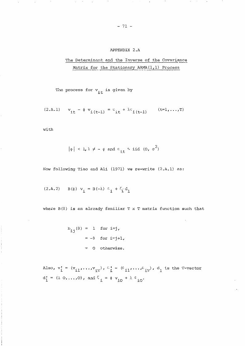
- 71 -

APPENDIX 2.A

The Determinant and the Inverse of the Covariance

Matrix for the Stationary ARMA(l,l) Process

The process for v. is given by1.t

(2.A.l)

with

E.it + A,Ei (t-l) (t=l, ... , T)

I~ I < 1, A :f - ~ and Eit

'U iid (0, a2

)

Now following Tiao and Ali (1971) we re-write (2.A.l) as:

(2.A.2) B (~) V.1.

where B(8) is an already familiar T x T matrix function such that

b .. (8)1.J

1 for i=j,

-8 for i=j+l,

o otherwise.

Also, vi = (vil,···,viT ), Ei = (Sil,···,s·iT)' d l is the T-vector

di = (1 0, .•. ,0), and t; i = ~ viO + A, S iO·

- 72 -

Furthermore, note that

( '\1 0 0

8 1 0

B- l (8) 82

8 0

I·T-l ·T-2

J8 8 1

and that detB(8) det B- l (8) 1.

Since we have assumed stationarity, s. is distributed independently of~

E:. wi th E ( S.) = 0 and~ ~

(2.A.3) E (s~)1.

2C5 K , say.

Now the covariance of (2.A.2) is

B(~) E(v.v~) B' (</»J. J.

Hence

v = .!-.-2 E (v. v ~ )~ ~

C5

or

(2.A.4)

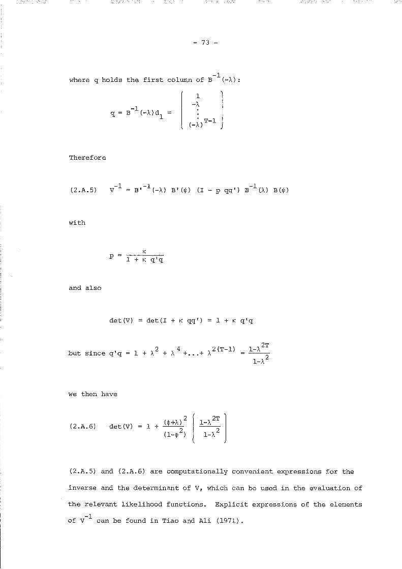
- 73 -

where g holds the first column of B-1

(-A,) :

Therefore

-1g = B (-A,)d

1

1-A,

(2 .A. 5)

with

and also

-1V

pK

1 + K g'g

det(V) det (I + K gg I ) 1 + K g'g

but since g'g

we then have

2 4 2 (T-l)1 + \ + \ +...+ \

1_\2T

1_\2

(2.A.6) det(V)

(2.A.5) and (2.A.6) are computationally convenient expressions for the

inverse and the determinant of V, which can be used in the evaluation of

the relevant likelihood functions. Explicit expressions of the elements

of v- lcan be found in Tiao and Ali (1971).

- 74 -

CHAPTER 3

THE ASYMPTOTIC PROPERTIES OF Q~1L ESTIMATORS IN A

TRIANGULAR MODEL WITH COVARIANCE RESTRICTIONS

3.1 Introduction

We have seen that the structure of dynamic models from panel data

is that of a simultaneous equations system of (T+l) equations where the

matrix of coefficients of the endogenous variables has a triangular

structure and the error covariance matrix is constrained. Generalising

the problem, this Chapter examines the asymptotic properties of quasi­

maximum likelihood estimators of triangular systems with general

restrictions in both the slope and the covariance coefficients. However,

we do not treat the case where there are restrictions relating the slope

coefficients to those in the covariance matrix, so that the results

presented below will primarily apply to random effects models with

unrestricted covariances between initial observations errors and the

remaining errors. In this context, it is natural to assume ~ll pre­

determined variables to be exogenous and therefore standard central

limit theorems for independent observations can be applied.

Normality is not imposed but we assume that the error vector is

generated by a distribution where the third order moments vanish and

the fourth order moments are finite. Indeed we are mainly concerned

with the role of non-normal kurtosis when estimating models with

covariance restrictions by quasi-maximum likelihood methods. This

role is more relevant, both for slope and covariance parameters

estimates, when covariance restrictions are enforced than when the

- 75 -

covariance matrix is left unrestricted. Distributions with long t~ils

are common in practice due to the presence of extreme observ~tions

in the sample, and they lead to large fourth moments relative to the

variances and covariances.

The structure of this Chapter is as follows. Section 3.2 states

the assumptions concerning the model and the quasi-log-likelihood

function, and derives limiting matrices of second partial deviatives

and products of first partials of the log-likelihood function when the

covariance matrix is not restricted and also when restrictions are

present. These results are extensively used below in deriving useful

expressions for the asymptotic variance matrix of the QML estimates when

normality holds (Section 3.3) and when the errors are possibly non-normal

(Section 3.4). It turns out that in the latter case imposing the

covariance restrictions may lead to an efficiency loss relative to the

estimators that leave the covariance matrix unrestricted. We give an

explicit condition on the fourth order moments to characterise this

situation. Finally, Section 3.5 discusses a simple two equation model

in order to illustrate our general results.

3.2 The Model and the Limiting Distribution of the QML Estimator

Yi is a n x 1 vector of dependent variables, and zi is a k x 1

vector of nonstochastic exogenous variables.

explained by

We assume that the y. are1

(3.2.1) B(8) y. + C(8)z.1 1

A(8)x.1

U.1

(i=l, ... ,N)

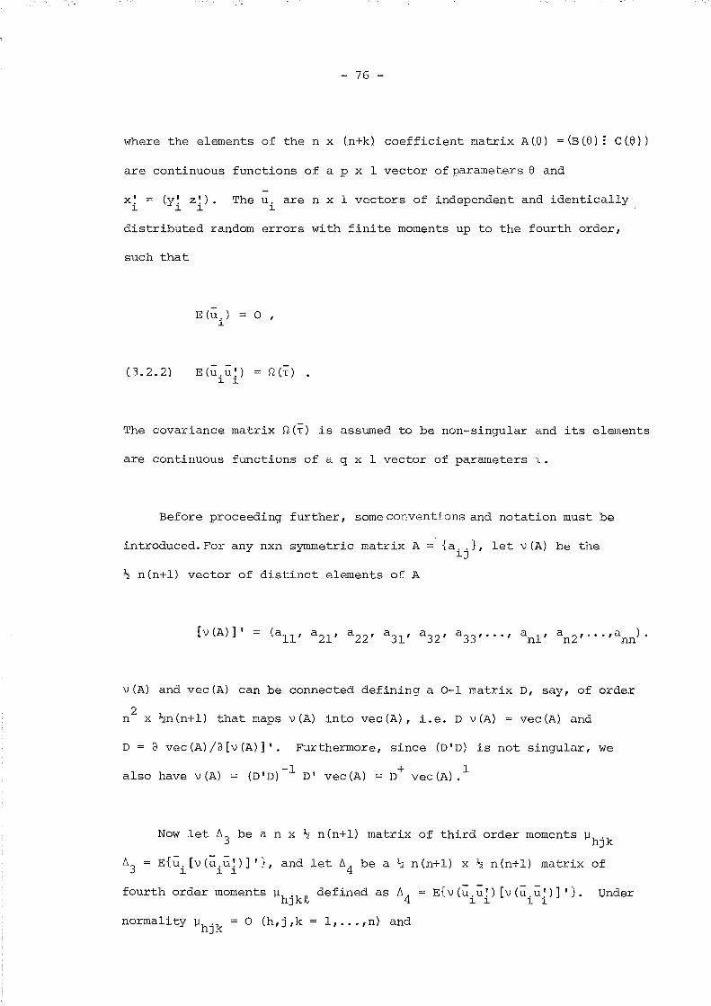
- 76 -

where the elements of the n x (n+k) coeft'icient matrix A(e) =(B(8): C(e»

are continuous functions of a p x 1 vector of parameters e and

x~ = (y~ z~). The u. are n x 1 vectors of independent and identicallyl l l l

distributed random errors with finite moments up to the fourth order,

such that

E(U,) 0,l

(3.2.2) $1 (T)

The covariance matrix Q(T) is assumed to be non-singular and its elements

are continuous functions of a q x 1 vector of parameters T.

Before proceeding further, some conventions and notation must be

introduced. For any nxn symmetric matrix A = {a .. }, let v (A) be thelJ

~ n(n+l) vector of distinct elements of A

[v (A) ] ,

veAl and vec(A) can be connected defining a 0-1 matrix D, say, of order

2n x ~n(n+l) that maps veAl into vec(A), Le. D veAl = vec(A) a.nd

D = 3 vec(A)/3[v(A)]'. Furthermore, since (D'D) is not singular, we

also have veAl = (D'D)-l D' vec(A) = D+ vec(A).l

Now let 63 be a n x ~ n(n+l) matrix of third order moments ].1hjk

/::'3 = E{u. [v(u,u~)] '}, and let /::'4 be a ~ n(n+l) x ~ n(n+l) matrix ofl l l

fourth order moments ].1hjk~ defined as /::'4

normality ].1hjk = 0 (h,j,k = l, ... ,n) and

E{v (u . u ~ ) [v (u . u ~ ) ] , }. Underl l l l

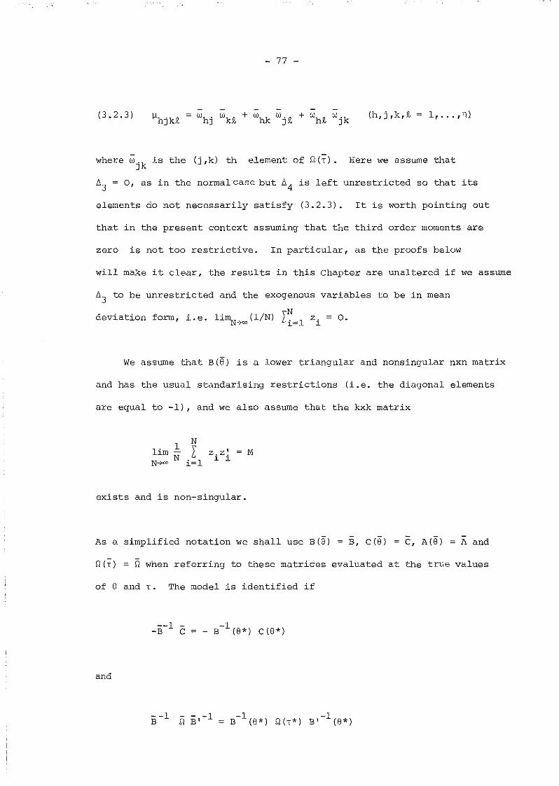
(3.2.3)

- 77 -

(h, j , k,.Q, 1, ... , n)

where wjk

is the (j,k) th element of S"2(t). Here we assume that

~3 = 0, as in the normal case but ~4 is left unrestricted so that its

elements do not necessarily satisfy (3.2.3). It is worth pointing out

that in the present context assuming that the third order moments are

zero is not too restrictive. In particular, as the proofs below

will make it clear, the results in this Chapter are unaltered if we assume

~3 to be unrestricted and the exogenous variables to be in mean

deviation form, i.e. li~+oo(l/N) 2.~=1 zi = o.

We assume that B(8) is a lower triangular and nonsingular nxn matrix

and has the usual standarising restrictions (i.e. the diagonal elements

are equal to -1), and we also assume that the kxk matrix

1 Nlim L z.z~ MN+oo N i=l 1. 1.

exists and is non-singular.

As a simplified notation we shall use B(8)-A and

S"2(t) = ~ when referring to these matrices evaluated at the true values

of e and T. The model is identified if

and

- -1B

- 78 -

for some S* and T* in the parameter space, implies that S* = e and

T* = T. However, since we are also interested in considering the quasi-

maximum likelihood estimator of S without imposing the restrictions in

the covariance matrix, we assume that the model is identified by mean of

the prior restrictions implicit in the matrix A(S) alone.

Let L be the gaussian log-likelihood function that leaves ~u

unrestricted, Lu

,N L withLi=l u,i

(3.2.4) L . (S,w)U,l

k ­o :!z log det ~ - ~ x~A' (S) ~-1 A(S) x.1 1

and let L be of the same form as L but in this case some set ofr u

constraints in ~ are enforced so that

(3.2.5) Lr

L (S, T)r

L (S,WeT))u

where V[~(T)], and accordingly we ~et w

The first order conditions for the estimators of e and T that maximise

L are given byr

(3.2.6)-1

R' (S) W (T) iI?l X'X) vec A(S) o

(3.2.7)-1 -1

G I (T) D I W (T) ® ~ (T)) vec [A (S) X' X A I (S) - ~ (T) ] o

where R(S)o vec A(S)

oS' , G(T)o W(T)---'---'- and X I X

OT Ix.x~

1. 1

(see Appendix 3.A). Let Sand T be the QML estimators.r

These solve

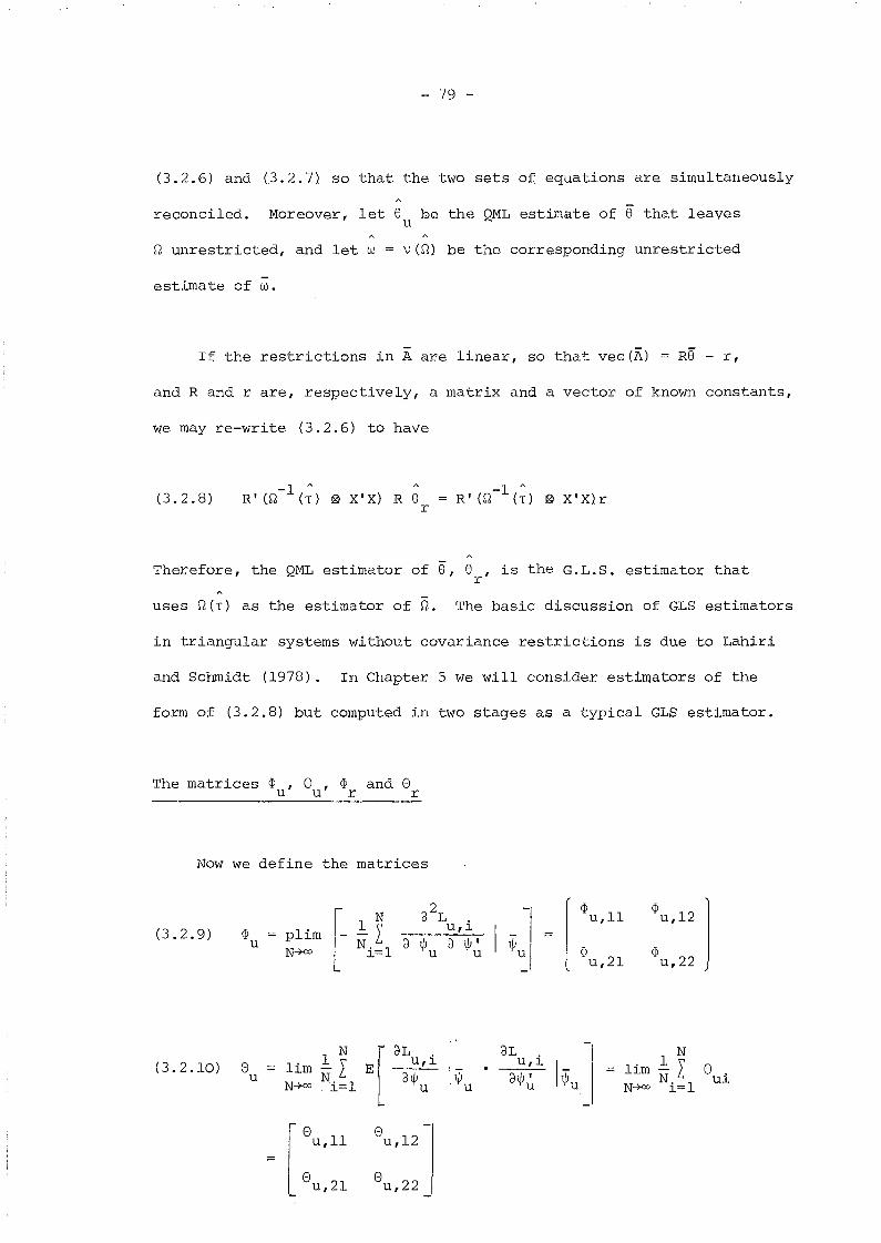
- 79 -

(3.2.6) and (3.2.7) so that the two sets 0;1'; equations are simultaneously

reconciled. Moreover, let e be the QML estimate of e that leavesu

Q unrestricted, and let w = \! (Q) be the corresponding unrestricted

estimate of iD.

If the restrictions in Aare linear, so that vec(A) Re - r,

and Rand r are, respectively, a matrix and a vector of known constants,

we may re-write (3.2.6) to have

(3.2.8)-1 A A

R' W (T) ~ X I X) R er

Therefore, the QML estimator of e, e , is the G.L.S. estimator thatr

uses Q(T) as the estimator of Q. The basic discussion of GLS estimators

in triangular systems without covariance restrictions is due to Lahiri

and Schmidt (1978). In Chapter 5 we will consider estimators of the

form of (3.2.8) but computed in two stages as a typical GLS estimator.

The matrices ~ , 8 , ~ and 8u u r r

Now we define the matrices

f1 N Cl

2L

r

~u,ll ~u,12

](3.2.9) ~ plim -I u,iu N. 1 Cl 1J; Cl 1J;' 1J;u ~ ~N-+co l= U u

u,21 u,22~

(3.2.10) 8u

=

1 NHrn -- IN-+co Ni=l

8 u,21

[

ClL .E· U,l

Cl1J;U

8u,12

8u,22

ClL .U,l

Cl1J;~

1 Nlim-I 8.N. 1 UlN-700 l=

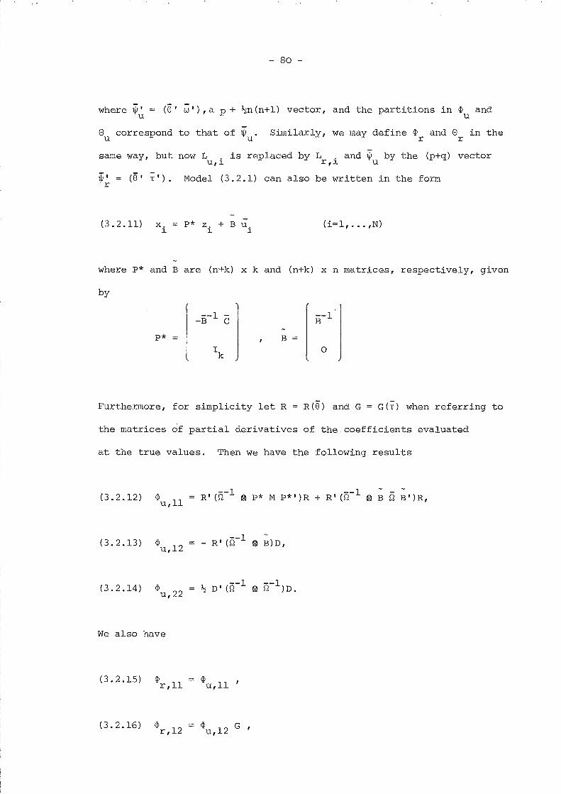
where ~,u

- 80 -

(8' w'),a p + ~n(n+l) vector, and the partitions in ~ andu

8 correspond to that of ~. Similarly, we may define ~ and 8 in theu u r r

same way, but now L ,is replaced by L ,and ~ by the (p+q) vectorU,l r,l u

~, = (8' T'). Model (3.2.1) can also be written in the formr

(3.2.11) x.1

p* Z, + B u.1 1

(i=l, ••• ,N)

where p* and Bare (n+k) x k and (n+k) x n matrices, respectively, given

by

I .1--1 - --1

-B C B

p* BI

k0

Furthermore, for simplicity let R = R(8) and G = G(T) when referring to

the matrices of partial derivatives of the coefficients evaluated

at the true values. Then We have the following results

(3.2.12)

(3.2.13)

(3.2.14)

~u,ll

~u,12

~u,22

We also have

(3.2.15)

(3.2.16)

~r,ll

~r,12

~u,ll

~ 2 G ,u,l

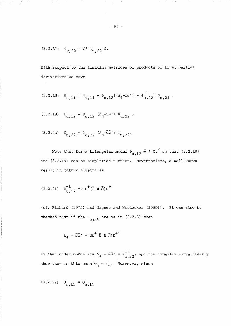
(3.2.17) ifJ r,22 G' ifJu ,22 G.

- 81 -

With respect to the limiting matrices of products of first partial

derivatives we have

(3.2.18 )

(3.2.19)

(3.2.20)

8u,ll

8u,12

8u,22

ifJ (L14-ww') ifJu,12 _ u,22

_ 2Note that for:a triangular model ifJ

u,12 w = 0, so that (3.2.18)

and (3.2.19) can be simplified further. Nevertheless, a well known

result in matrix algebra is

(3.2.21)

(cf. Richard (1975) and Magnus and Neudecker (1980)). It can also be

checked that if the llhjk£ are as in (3.2.3) then

L1 4 = ww'+ - - +,

+ 2D (Si ~ Si) D

so that under normality L14 - ww' -1= ifJu ,22' and the formulae above clearly

show that in this case 8 = ifJ. Moreover, sinceu u

(3.2.22) 8r,ll 8u,ll

(3.2.23)

(3.2.24)

(3r,12

(3r,22

(3 Gu,12

G' (3 Gu,22

- 82 -

also (3r

~ under normality.r

The proofs of (3.2.12) to (3.2.20) and (3.2.22) to (3.2.24) are given

in Appendix 3.A.

Having assumed that our model is identified, by using the

arguments in Sargan (1975), it follows that the quasi-maximum likelihood

estimators of 8 and T obtained by maximising L (8,T) are consistentr

even when the u. are not normally distributed.l.

A

Now since (oL /(1)J ) 11)Jr r r o by the definition of 1)Jr' an exact first

order Taylor series expansion of oL /(1)J about 1)Jr yieldsr r

(3.2.25)1 NN I

i=l

1 N-IIN i=l

where 1)J* lies between ,I, and 1)J .r ~r r

Since oL ./(1)J I~ are independently distributed random vectors withr,l. r r

zero mean' and covariance matrices (3 ., given our assumptions,r,l.

standard (Liapunov) central limit theorem (e.g. see Rao (1973), p.147)

ensures that

(3.2.26) 1

IN

N

Li=l

oL. dr,l.

1

- +N(O, (3).(1)Jr 1)Jr r

- 83 -

Finally, if we note that since 1jJr is consistent for ~r so is 1jJ~

and thus plimN

{- (l/N) I~ 1 (a 2L . /a1jJ a1jJ I) I",*} 1', using the Cramer+00 1= r,l r r ~ r

rlinear transformation theorem we have

(3.2.27)

with

d- ~ ) -+ N (0, W )

r r

(3.2.28) Wr

-1l' .

r

Clearly, the same is true for 1jJu (8 w) I as it can be regarded asu

a specialisation of the previous result to weT) = T. So

(3.2.29)

with

d- ~ ) -+ N(O, W )

u u

(3.2.30) wu

-1l' .

u

3.3 The Asymptotic Variance Matrix of the QML Estimators when the

Errors are Normal

Under normality, in view of the equivalence between l' and El (theyr r

are, respectively, the hessian and outer product forms for the information

matrix), the asymptotic variance matrix (AVM) of 1jJ reduces to Wr r

In what follows we report some results concerning the partitions of

-1 -1l' and l' . Letting

u r

-1l' .

r

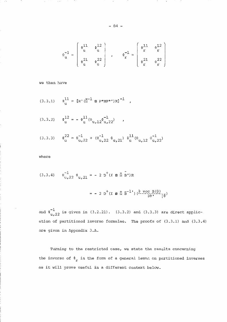
- 84 -

<I> 11 <I> 12

-1u u

<I>u

<I> 21 <I>22u u

-1<I>

r

we then have

(3.3.1) <I> 11 [R I (~-l ~ P*MP* I) R]-lu

(3.3.2) <I> 12 11 -1<I> (<I> 12<I> 22)u u u, u,

(3.3.3) <I> 22 -1 -1<I>u,21) <I>11 (<I> -1

<I>u,22 + (<I>u,22 u,12 <I>u,22)u u

where

(3.3.4) <I>-l <I>u,22 u,21

-1and <I>u,22 is given in (3.2.21). (3.3.2) and (3.3.3) are direct applic-

ation of partitioned inverse formulae. The proofs of (3.3.1) and (3.3.4)

are given in Appendix 3.A.

Turning to the restricted case, we state the results concerning

the inverse of <I> in the form of a general lemma on partitioned inversesr

as it will prove useful in a different context below.

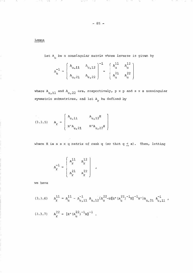
- 85 -

Lemma

Let A be a nonsingular matrix whose inverse is given byu

A-1 All A

12

]A

u,12-1

u,ll u uA

A2l

A22u

A Au,2l u,22 u u

where Au,ll and Au ,22 are, respectively, p x p and s x s nonsingular

symmetric submatrices, and let A be defined byr

(3.3.5) Ar

AU ,12H 1

H'Au ,22H J

where H is a s x q matrix of rank q (so that q < s). Then, letting

rAll A

12

-1r r

A lrA

2lA

22r r

we have

(3.3.6)

(3.3.7)

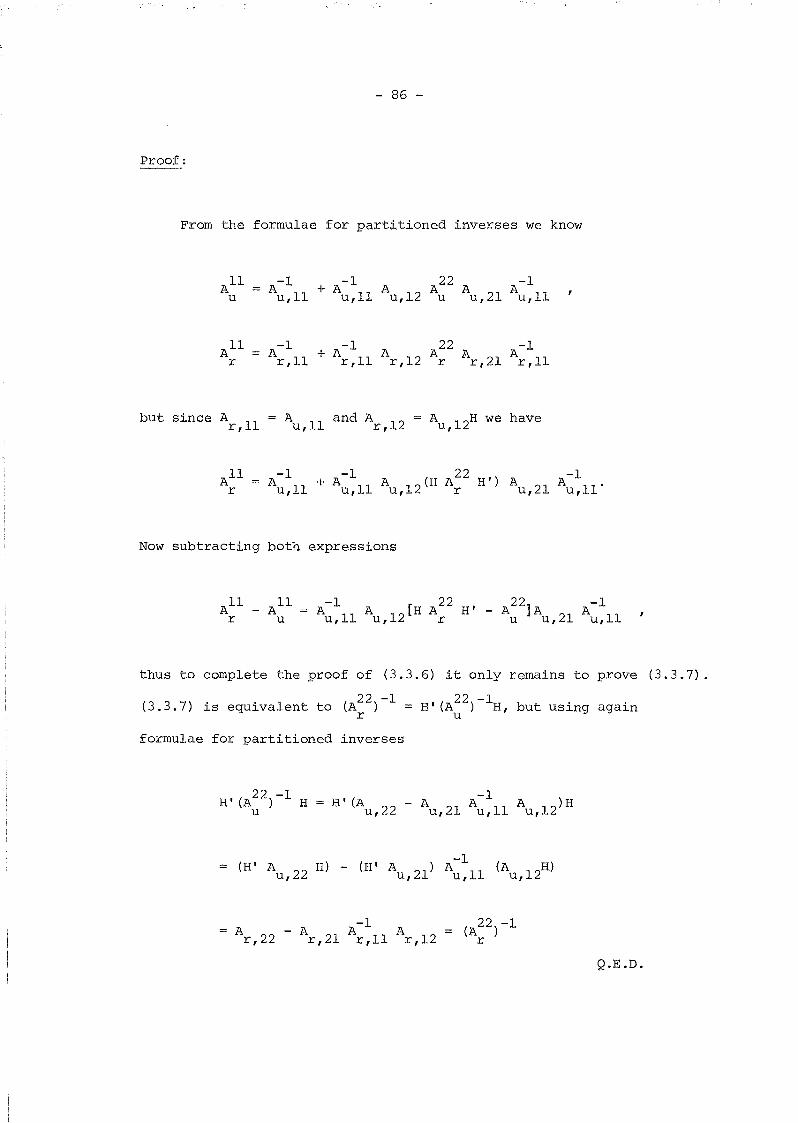
- 86 -

Proof:

From the formulae for partitioned inverses we know

-1 -1 A A22 -1A + Au,ll 12 A 21 A 11u,ll u, u u, u,

-1 A- l A A22 -1Ar,ll + 11 12 A 21 A 11r, r, r r, r,

but since Ar,ll

All A- l + A- l A (H A22 H') A A- lr u,ll·· u,ll u,12 r u,2l u,ll·

Now subtracting both expressions

All 11

- Ar u

thus to complete the proof of (3.3.6) it only remains to prove (3.3.7).

(3.3.7) is equivalent to (A22 )-1 = H' (A22 )-lH, but using againr u

formulae for partitioned inverses

(H' A H) - (H' A ) A-l

(Au,12H)u,22 u,21 u,ll

Ar,22

A A- l Ar,21 r,ll r,12

Q.E.D.

- 87 -

Note that

(3.3.8)

22 -1 -1 22 -1whore P = a[H' (A ) Hl Il' (A ) .

A u uGo that if A// is positive

u

definite (3.3.8) will be positive semi-definite.

Also note that an alternative expression for (All)-l is given byr

The proof of (3.3. 6a) paralels that of (3.3.6), but now we use

and

-1A - A A Ar,ll r,12 r,22 r,21

Au,ll A 12H (H'A 22H)-lH'A 21u, u, u,

Au,ll

A A- l Au,12 u,22 u,21

subtracting both expressions the result follows.

In view of this Lemma, for-restricted models we have

(3.3.9) <I:>Hr

<I:>-l <I:> {<I:>22u,ll u,12 u

(3.3.10) <I:>22r

- 88 -

11 11When normality holds, cP and cP are the asymptotic variance

u r

matrices of the QML estimators of e based on Land L , respectively,u r

e and e Since {cp22 - G[G' (cp22) -lG] -lG'} is positive semi-definite,u r u u

(3 3 9) '1' h ('1'.11 ",,11), " , d f' . t S th t.• ~mp ~es t at.~ - ~ ~s pos~t~ve sem~- e ~n~ e. 0 au r

3under normality e is efficient relative to e. This result wasr u

first shown by Rothenberg and Leenders (1964) who analised the cases

where ~ is either a diagonal matrix or is completely known, and it

was further investigated in Rothenberg (1973). Recently, a similar

result for simultaneous (non-triangular) models has been given an

instrumental variables interpretation, in the sense that when some

a priori information on ~ is available, the ML estimator is able to form

better instruments for the endogenous variable (cf. Hausman, Newey and

Taylor (1983)). Nevertheless, for a triangular model the QML estimator

solves a set of "generalised" least squares equations and so, in this

case, the efficiency . gain of e with respect to e can be regarded asr u

a direct consequence of the efficiency gain of ~(T) with respect to ~

in estimating~. In particular, if Q is completely known, then

cp22 = 0 so that (3.3.9) becomesr

cpUr

-1 22 -1cp 11 cp 12(~ )CP 21 ~ ·11u, u, u u, u,

cp11u

-1cpu,ll

3.4 The Asymptotic Variance Matrix of the QML Estimators when the Errors

are Possibly Non-normal

and 1fJr

are given by

-1~ , respectively.

r-1

~ and Wu r~-l 8

u u

When the errors are not normal the AVM's of ,I,'l'u

cp-l 8r r

the general formulae Wu

To be more specific, this will be the case when the fourth order moments

- 89 -

do not satisfy (3.2.3) as this is the only non-normal feature of the

actual distribution that is relevant in the present context.

Starting with ~-unrestricted estimators, the partition of W isu

given by

(3.4.1)

(3.4.2)

(3.4.3)

Wu,ll

Wu,12

Wu,22

iPHu

h An, th 1 fAd l't 1.' .e. An = w-w-, + ffi-l

were u4

1.S e va ue 0 u4

un er norma 1. y, u - ~4 u,22

Proofs:

- 90 -

and simply noting that

rq)u,12

(q)ll. q)12 )(3.4.4) I o ,

u u

l q)u,22

we have

Wu,ll

q)ll (q)ll) -1 q)llu u u

Equally, to prove (3.4.2) we write

Wu,12 o

o

o

q)u,12

+q)u,22

but using again (3.4.4), we have

Wu,12

q)ll (q)1l) -1 q)12u u u

Finally, Wu ,22 is given by

[(q)ll) -1

')

0

I(q)21 • q)22)u

Wu,22 u u

0 0 J(

q)12

Iq)u,12 u

+ (11 - WW I ) (q)u , 21 . q) )q)22l q) 4 u,22

u,22 u

- 91 -

Using that

r1>u,12

](1)21 : 1> 22) Iu u

l 1>u,22

we have

W 1>21 (1)11) -1 1>12 + (b, - ww·)u,22 u u u 4

but in view -1 1>22 1>21 (1)11) -1 1>12 Wu ,22 equalsthat 1>u,22 u u u u '

1>22 -1 (b, - ww' )Wu,221> +

u u,22 4

what proves (3.4.3).

(3.4.1) shows that the A.V.M. of e (i.e. the QML estimator of 8u

based on Q unrestricted) equals 1>11 independently of non-normality.u

This is not the case, however, for the A.V.M. of W (i.e. the

unrestricted QML estimator of w): for a leptokurtic distribution

(i.e. b,4 - b,~ > 0, where the inequality sign is taken in the usual

matrix sense) the A.V.M. of w will be larger as compared with the

A.V.M. of w under normality, whereas for a platykurtic distribution

the conclusion will be the opposite. Nevertheless, the first case is

more likely to occur in practice than the latter, as the presence of

outliers among the sample observations tends to increase the value of

fourth order moments above their gaussian levels.

- 92 -

Turning to QML estimators based on ~ restricted, we have the

following results:

(3.4.5) Wr,ll

where

(3.4.6) Wr,22

or equivalently,

(3.4.6a) Wr,22

The proofs of (3.4.5), (3.4.6) and (3.4.6a) are given in Appendix 3.B.

The expression for Wr,ll in (3.4.5) has important implications.

In the first place, notice that the A.V.M. of e , contrary to whatr

happens with e , does depend on non-normality. But more relevant, nowu

it is not generally guaranteed that the QML estimator of e that takes

into account the constraints in ~ is efficient relative to the QML

estimator of e that leaves ~ unrestricted. Actually, if the fourth

order moments of the distribution of the errors are large enough, it

can be the case that imposing the constraints in ~ implies an efficiency

loss with respect to e. We state this result formally in the followingu

proposition.

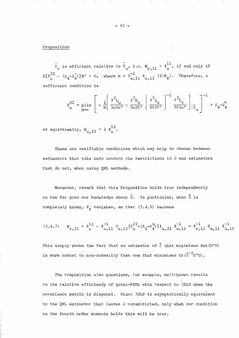
- 93 -

Proposition

er is efficient relative to eu' i.e. Wr,ll",11

< '" ,U

if and only if

sufficient condition is

q:,22 r-l[ d2L d2

L [ d2L r d2

L ]r' lJu u u u

I~u -'plim 3WdW' dWde' de de' de dW I

> 6 -6u L NI.

4 4N-+<x>

. 1 1 2 ",22.or equlva ent y, Wu ,22 < "'u

These are verifiable conditions which may help to choose between

estimato~s that take into account the restrictions in ~ and estimators

that do not, when using QML methods.

Moreover, remark that this Proposition holds true independently

on how far goes our knowledge about~. In particular, when ~ is

completely known, Pq:, vanishes, so that (3.4.5) becomes

(3.4.7) Wr,llq:,-l 0 q:,-lu,ll u,ll u,ll

This simply shows the fact that an estimator of e that minimises det(U'U)

is more robust to non-normality than one that minimises tr(~-lu,U).

The Proposition also questions, for example, well-known results

on the relative efficiency of quasi-FIML with respect to 3SLS when the

covariance matrix is diagonal. Since 3SLS is asymptotically equivalent

to the QML estimator that leaves ~ unrestricted, only when our condition

on the fourth order moments holds this will be true.

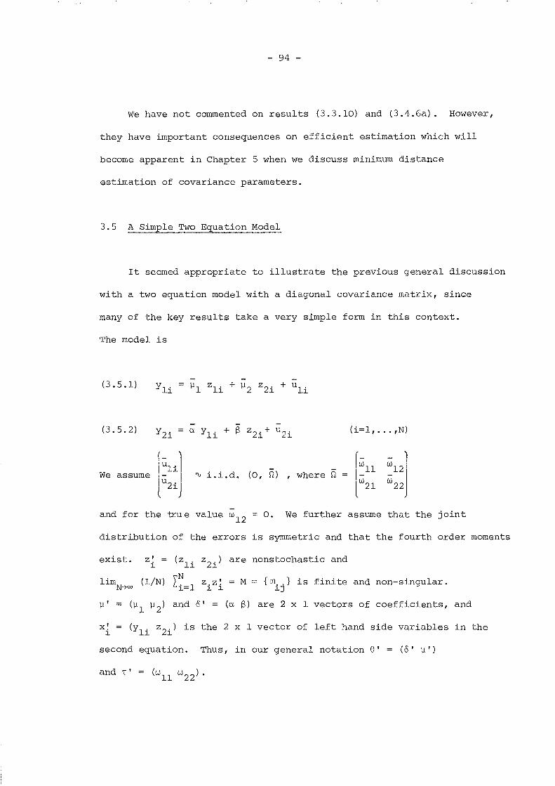
- 94 -

We have not commented on results (3.3.10) and (3.4.6a). However,

they have important consequences on efficient estimation which will

become apparent in Chapter 5 when we discuss minimum distance

estimation of covariance parameters.

3.5 A Simple Two Equation Model

It seemed appropriate to illustrate the previous general discussion

with a two equation model with a diagonal covariance matrix, since

many of the key results take a very simple form in this context.

The model is

(3.5.1)

(3.5.2) Y2i = a Yli + (3 z2i + u2i (i=l, ... ,N)

~li](-

~12]IWll

We assume tU LLd. (0, m , where Q 1-u2i lW 21w

22

and for the true value w12

= o. We further assume that the joint

distribution of the errors is symmetric and that the fourth order moments

Z2i) are nonstochastic andexist. zi = (zli

(l/N) L~=l z.z~1. 1.

M = {m.. } is finite and non-singular.1.J

fl'

x'i

(fll

fl2

) and 0' = (a (3) are 2 x 1 vectors of coefficients, and

(Yli z2i) is the 2 x 1 vector of left hand side variables in the

second equation. Thus, in our general notation e' = (0' fl')

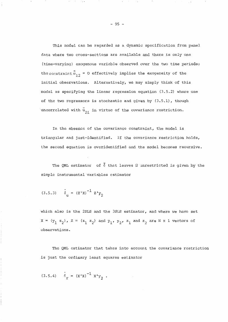
- 95 -

This model can be regarded as a dynamic specification from panel

data where two cross-sections are available and there is only one

(time-varying) exogenous variable observed over the two time periods;

theconstraintw12 = 0 effectively implies the exogeneity of the

initial observations. Alternatively, we may simply think of this

model as specifying the linear regression equation (3.5.2) where one

of the two regressors is stochastic and given by (3.5.1), though

uncorrelated with u2i

in virtue of the covariance restriction.

In the absence of the covariance constraint, the model is

triangular and just-identified. If the covariance restriction holds,

the second equation is overidentified and the model becomes recursive.

The QML estimator of 8 that leaves Q unrestricted is given by the

simple instrumental variables estimator

(3.5.3) 8u

-1(Z'X) Z'y

2

which also is the 2SLS and the 3SLS estimator, and where we have set

observations.

The QML estimator that takes into account the covariance restriction

is just the ordinary least squares estimator

(3.5.4) 8r-1

(X'X) X'y2

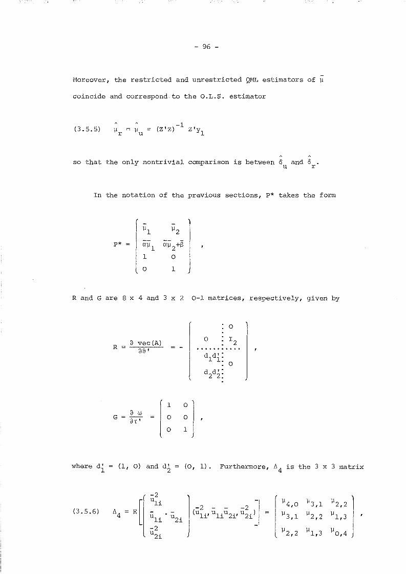
- 96 -

Moreover, the restricted and unrestricted QML estimators of ~

coincide and correspond to the O.L.S. estimator

(3.5.5) ~u(Z' z) -1 z 'y

1

so that the only nontrivia1 comparison is between 0 and 8u r

In the notation of the previous sections, p* takes the form

p* ==

~2

a~2+i3

o

1

Rand G are 8 x 4 and 3 x 2 0-1 matrices, respectively, given by

r

· 0')

Ia vec(A) 0 · 1 2

R ae' ...........I d 1di:

l · 0d 2d2:

r1 0

1a wG aT' 0 0

l 0 1 J

where di (1, 0) and d2 (0, 1) . Furthermore, 1:14 is the 3 x 3 matrix

Err-2 (Uli

1 - I ~4,0 ~3,1 ~2,2-2 - - -2(3.5.6) 1:14 (Uli, u liu 2i' u 2i ) =

l~3,1 ~2,2 ~1,3

L[u1i u

2i-2

J-

u2i

~2,2 ~1,3 ~0,4

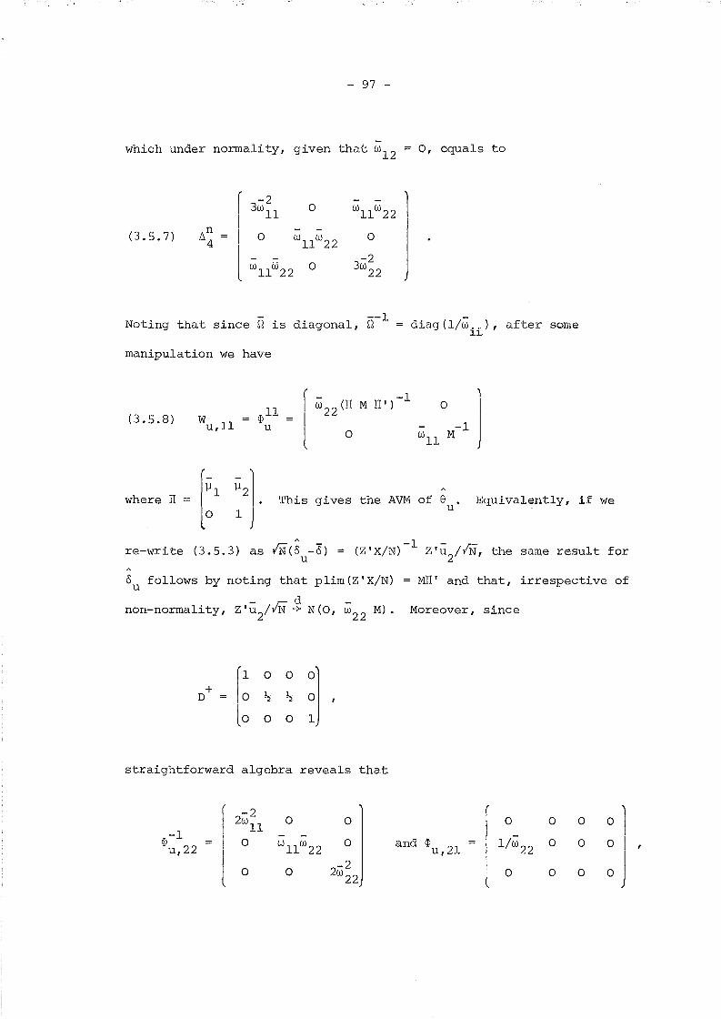
- 97 -

which under normality, given that w12 = 0, equals to

(3.5.7) /::,.n4

--1Noting that since ~ is diagonal, ~

manipulation we have

diag (l/w .. ), after someJ..J...

(3.5.8) Wu,llcpU

u - 0 -1 JI

wll

M

Equivalently, if wewhere IT = ["1 "21. This gives the AVM of 8o 1 J u

re-write (3.5.3) as !N(8u-8) = (Z'X/N)-l Z'u

2/!N, the same result for

8 follows by noting that plim(Z'X/N) = MIT' and that, irrespective ofu

_ cd -non-normality, Zl u2/ vN + N(O, w

22M). Moreover, since

o 0

o 0

straightforward algebra reveals that

r-2 (

12w u 0 0 0 0 0 0-1cp I 0 w

llw

220 and cp 1/w22

0 0 0 Iu,22

lu,21

J-2

0 0 2w22 0 0 0 0

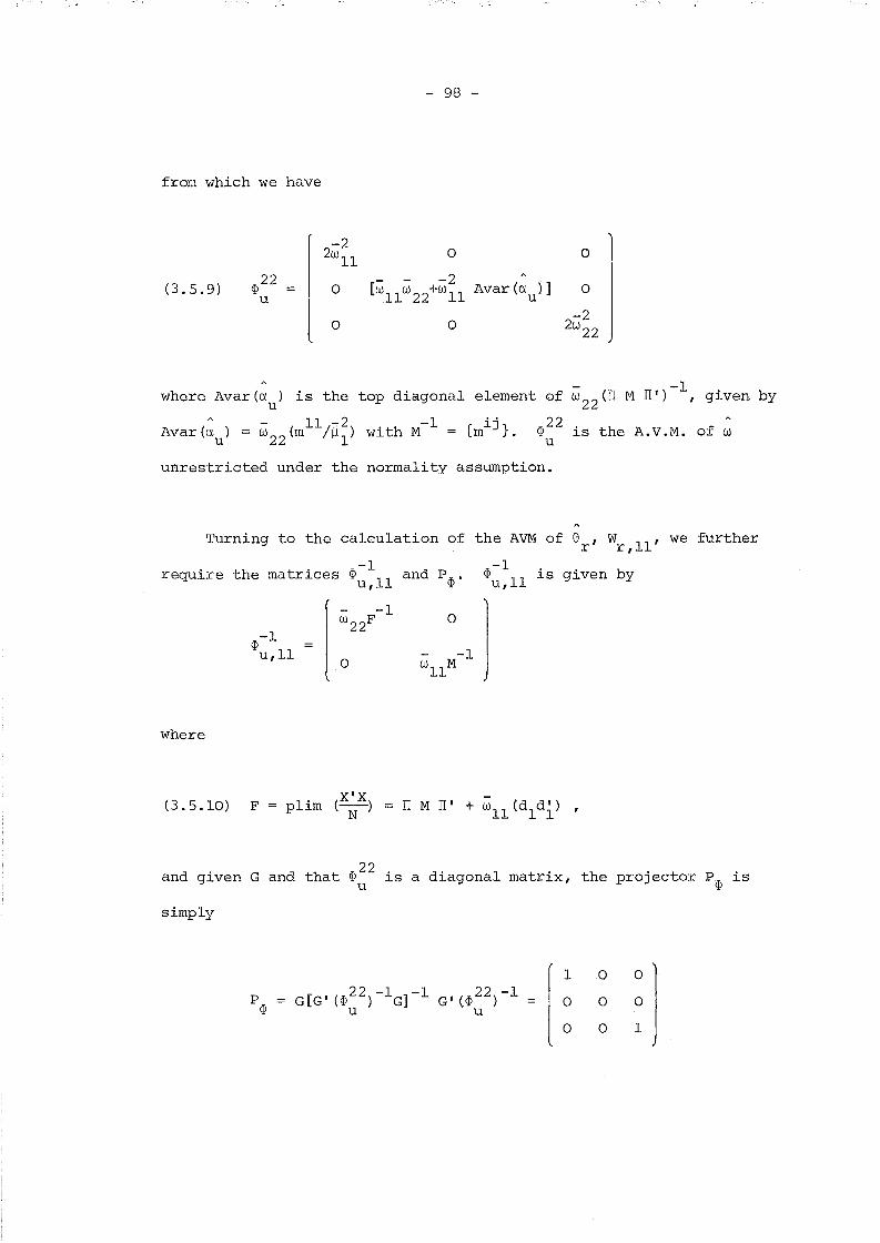
- 98 -

from which we have

r

-2 I2wll

0 0

<IJ22 - - -2 Avar(a )](3.5.9) 0 [(jJll

w22

+wll

0u

lu

-20 0 2w

22

where Avar(a ) is the top diagonal element ofu

- 11 72 -1 ij 22Avar(au ) = w

22(m /~l) with M = {m }. <IJ

u

unrestricted under the normality assumption.

-1w22

(IT M IT') , given by

is the A.V.M. of w

Turning to the calculation of the AVM of e ,W 11' we furtherr r,-1

require the matrices <IJu,ll and P<IJ.-1

<IJ is given byu,ll

-1<IJu,ll

where

o

o

(3.5.10) F

and given G and that <IJ~2 is a diagonal matrix, the projector P<IJ is

simply

1

o

o

o

o

o

o

o

1

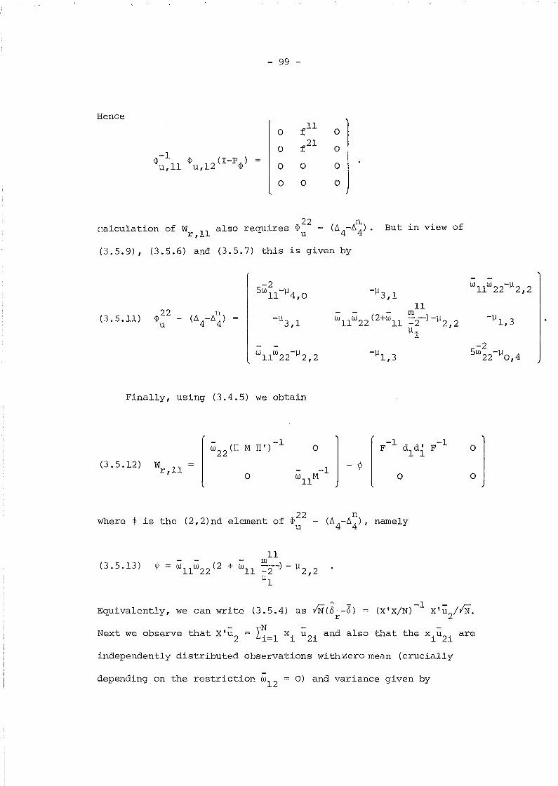
- 99 -

Hence

0 fll 0

0 f2l 0-1

.pu,12(I-P.p) l.p ==u,ll 0 0 0

0 0 0

"'U22 - (,A

4_A

n'4'). " fcalculation of Wr,ll also requires ~ ~ D But In Vlew 0

(3.5.9), (3.5.6) and (3.5.7) this is given by

-2 WllW22-).l2,25wll-]14,0 -).l3,1

11.p22 ,n

Wll

w22

(2+Wll

m(3.5.11) (!14-~4) -]13,1 - -)-]1 -]11,3u -2 2,2

]11

-2W11W22-]12, 2 -]11,3 5W 22-]10,4

Finally, using (3.4.5) we obtain

W22

(IT M n,)-1 0

]-1

dldi-1

0F F

(3.5.12) Wr,ll - -1 - <P0 W

11M 0 0

where <P is the (2,2)nd element of .p22u

(3.5.13)11

m=-2) -]12 2]1 ,

1

Equivalently, we can write (3.5.4) as /N(8 -8)r

- \'N -Next we observe that X'u2 == ~i=l xi u 2i and also that the x,u

2' are

l l

independently distributed observations with zero mean (crucially

depending on the restriction w12

== 0) and variance given by

- 100 -

(3.5.14) r

A

Therefore, IN(o - 8)r

w22

F-l r F-1 = w22

(IT

1 N(O, w22

F-1 r F-l ). It can be shown that

-1 -1 -1M IT') -~. F dldi F as in (3.5.12). Remark

that under normality or, more generally, if uli

and u2i

are independent,

- - - 11-2~2,2= w

llw22 so that r F and also ~ = wllw22 (1 + wllm /~l) which is

clearly non-negative.

However, in general

(3.5.15) AVAR(O)r

and therefore

AVAR(O ) < AVAR(O )r u

if any only if~. > 0 or

11m

(3.5.16)

-2 -2E (u

liu

2i)

-----<2+w11 -2

~l

-1 -1given the fact that F d

1di F is positive semi-definite. (3.5.16)

particularises to this example the necessary and sufficient condition

stated in the Proposition of Section 3.4.

- 101 -

NOTES

1 D is the duplication matrix whose properties are extensively

.. +studied in Magnus and Neudecker (1980), and D is the Moore-Penrose

inverse of D.

2 In view of (3.2.13) we have ~u,12 w R' Cfi- l0 ~)D iD =

- R' vecCB'). A typical element of this

vector is given by

- [vec (A .)], vec CB' )J

- tr CA '. B')J

aA (8)where A. = = (B.

J ae. le JJ

and

--1Cj ),> (;;i=l, ... ,p). But B A j = B B j ~ .

--1since B. is strictly lower.triangular and B is lower triangular,

]

--1 --1·the diagonal elements ofB Bj are all zero so that tr(B Bj) 0

(j=l, •.• ,p).

3 Incidentally, notice that in a multivariate regression model

(i.e. where B is a unit matrix) 8 and 8 are equivalent, as inu r

this case ~ = 0 so that ~ll ~ll.u,12 r u

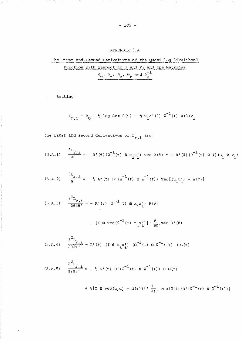
- 102 -

APPENDIX 3.A

The First and Second Derivatives of the Quasi-log-likelihood

Function with respect toe and T, and the Matrices

~ , ~ , Su' S and ~-lu r r u

Letting

L .r,]. k ­o ~ log det neT) - ~ x ~ A I (8) n-1 (T ) A (8 ) x .]. ].

the first and second derivatives of L . arer,].

(3.A.l)dL .r,].

d8- R' (8) en-leT) ~ x.x~) vec A(8)

]. ].

-1- R' (8) en (T) ~ I) (u. 2 x.)

]. ].

(3 .A. 2)

(3 .A. 3)

(3 .A. 4)

(3 .A. 5)

dL .r,].dT

2d L .r,].

d8 d8 I

2d L .r,].d8 dT I

2d L .r,].dTdT '

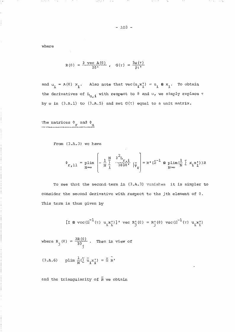
- 103 -

where

R (8)~ vec A(8)

d8 I

dW (1')dT I

and U o = A(8) X O '

1. 1.Also note that vec Cu 0 x ~) = u 0 ~ x 0 • To obtain

1. 1. 1. 1.

the derivatives of L 0 with respect to 8 and w, we simply replace TU,1.

by W in (3.A.l) to (3.A.5) and set GCT) equal to a unit matrix.

The matrices ~ and ~r u

From (3.A.3) we have

~r,ll

plimN-+oo

1 N-IN 1

2d L 0

r,1.

dEl d8 I IJ. ] = R' (i1-1 ~ plim(~ I x.x~))R~r N-+oo 1. 1.

To see that the second term in (3.A.3) vanishes it is simpler to

consider the second derivative with respect to the jth element of 8.

This term is thus given by

-1[I ~ vec W (1') u 0 x ~ ) ] I vec R! (8) =

1. 1. J

where R. (8)CJR (8)

Then in view ofd8J j

(3 .A. 6) plim l(I UoX ~) = r2 B 'N 1. 1.

and the triangularity of B we obtain

-1R! (8) vec W (T) u 0 x ~ )

J 1. 1.

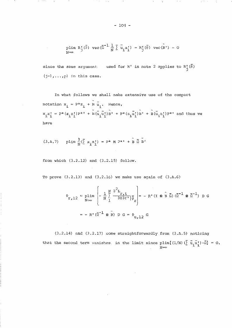
- 104 -

--1 1 \plim R~ (8) vec (r2 -N· L u.x~)

J ~ ~N-+oo

Rj (8) vec(B I ) o

since the same argument

(j=l, ... ,p) in this case.

used fOr R I in note 2 applies to R ~ (8)J

In what follows we shall make extensive use of the compact

-notation x. = P*z. + B u.. Hence,

~ ~ ~

x.x~~ ~

have

P*(Z.Z~)p*I + B(u.U~)B' + P*(z.u~)B' + B(u.Z~)P*' and thus we~ ~ ~ ~ ~ ~ ~ ~

(3.A.7) pl {m 1.(\ x x I)-'- N L ..~ ~

p* M p*I + B r2 B '

from which (3.2.12) and (3.2.15) follow.

To prove (3.2.13) and (3.2.16) we make use again of (3.A.6)

q,r,12

( 2 ]1 N 3 L .

plim [- NI 3~a~' I~ =N-+oo 1 r

- RI (f.i- l ~ B) D G q, Gu,12

(3.2.14) and (3.2.17) come straightforwardly from (3.A.5) noticing

that the second term vanishes in the limit since plim [ (l/N) (L u.u~ )-f.il o.N-+oo ~ ~

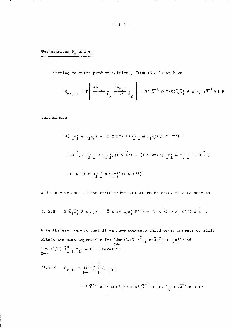
- 105 -

The matrices 8 and 8r u

Turning to outer product matrices, from (3.A.l) we have

8 = Eri,ll

furthermore

dL ,r,~

dS I~r

(I ~ p*) E (u ,u~ ~ z, z ~ ) (I ~ P*') +~ 1 1 1

(I ~ B)E(u,u: ~ u,;:;:~) (1 ~ B') + (I ~ P*)E(u,u~ ~ z,u~) (I ~ B')1 1 ~ 1 1 1 1 1

+ (I ~ B) E(u.u~ ~ u,z~) (I ~ P*')1 1 1 1

and since we assumed the third order moments to be zero, this reduces to

(3 .A. 8) E(U,u~ ~ x,x~)1 1 1 ~

(~ ~ p* z,z~ P*') + (I ~ B) D ~4 D' (I ~ B').1 1

Nevertheless, remark that if we have non-zero third order moments we still

obtain the same expression for lim{(l/N) IN E(u u' ~ x,x~)} ifi=l i ill

N+x>

lim{ (l/N) I~=l zi} = o. ThereforeN+x>

(3.A.9) er,ll

1 Nlim - '\ 8

N L. ri,llN+x> 1

- 106 -

what in view of (3.2.12) and (3.2.13) can be written as

8r,ll

Now to prove (3.2.18) it suffices to show that

(3.A.IO) R' ($1-1 ~ ~ rl B')R <I? <I?-l <I?u,12 u,22 u,21

From (3.2.13) and (3.2.21) we have

<I? <I?-l <I?u,12 u,22 u,21

Now using properties from Magnus and Neudecker (1980)

+ - - +, ,2 DD W ~ rl)D D

- - +' ,2 W ~ rl)D D

where K is the commutation matrix. Thus we have

(3.A.H) <I? <I?-l <I?u,12 u,22 u,21

- 3 vec(A') .The second term simplifies to R' (B' ~ B) ( 38' ) whlch equals zero

for B lower triangular. This establishes (3.A.IO) and indeed <3.2.18) and

(3.2.22). Incidentally, note that

23 log det B(8)

3838 'R' (B' §Il ~,) (d vec (A') )

38 '

which is non-zero if B is not triangular. This is a third extra term that

appears in the formula for <l?u,ll when the model is not triangular, in

- 107 -

order to take account of the Jacobian term in the quasi-log-likelihood

function. But as (3.A.ll) makes clear the result in (3.2.18) is still

valid in non-triangular cases.

Considering the off-diagonal terms in 8 and 8 , we haver u

8ri,12 I dL .r,1.

E de I~l r

dL .r,1.

dT I Iijjr

1 R' (~-l 0 I) (- - 0 - --1 0 ~-l) DG'2 OG lI.\l E u.u~ lI.\l x.u~) (Si lI.\l OG1. 1. 1. 1.

and given that E(U.X~)1. 1.

obtain

(I ~ B)D ~4 D' we

8 r,121 N

Hm - I 8N ri,12N-+ro 1

- --1+ ~ R' vec(B') [vec(Si )] I DG .

The second term vanishes since R' vec(B')

(3.2.13) and (3. 2.14)

o (see note 2), and using

8 r,12 ~ ~4 ~ Gu,12 u,228 G

u,12

what proves (3.2.19) and (3.2.23).

- 108 -

Finally, noting that

we have

i'i) [vec (u. u~~ ~

D(!'I - wW')D',4

E(U.U~ ~ U.U~) - vec(i'i) [vec(i'i)]'~ ~ ~ ~

8ri,22 l

(dL .r,~

E dT 10r

dL .r,~

dT' 10r

and in view of (3.2.14), then (3.2.20) and (3.2.24) follow.

-1The matrix <I>

u

In order to prove (3.3.1) we use the partitioned inverse result

and this yields

[R'(i'i- l ~ P*MP*')R + R'(i'i- l ~~. Q B')R

But in view of (3.A.10) the last two terms cancel and the result is proved

(our previous remark also applies here: this result is still valid if the

model is not triangular). (3.3.4) is proved in a similar way to (3.A.10).

In this case we have

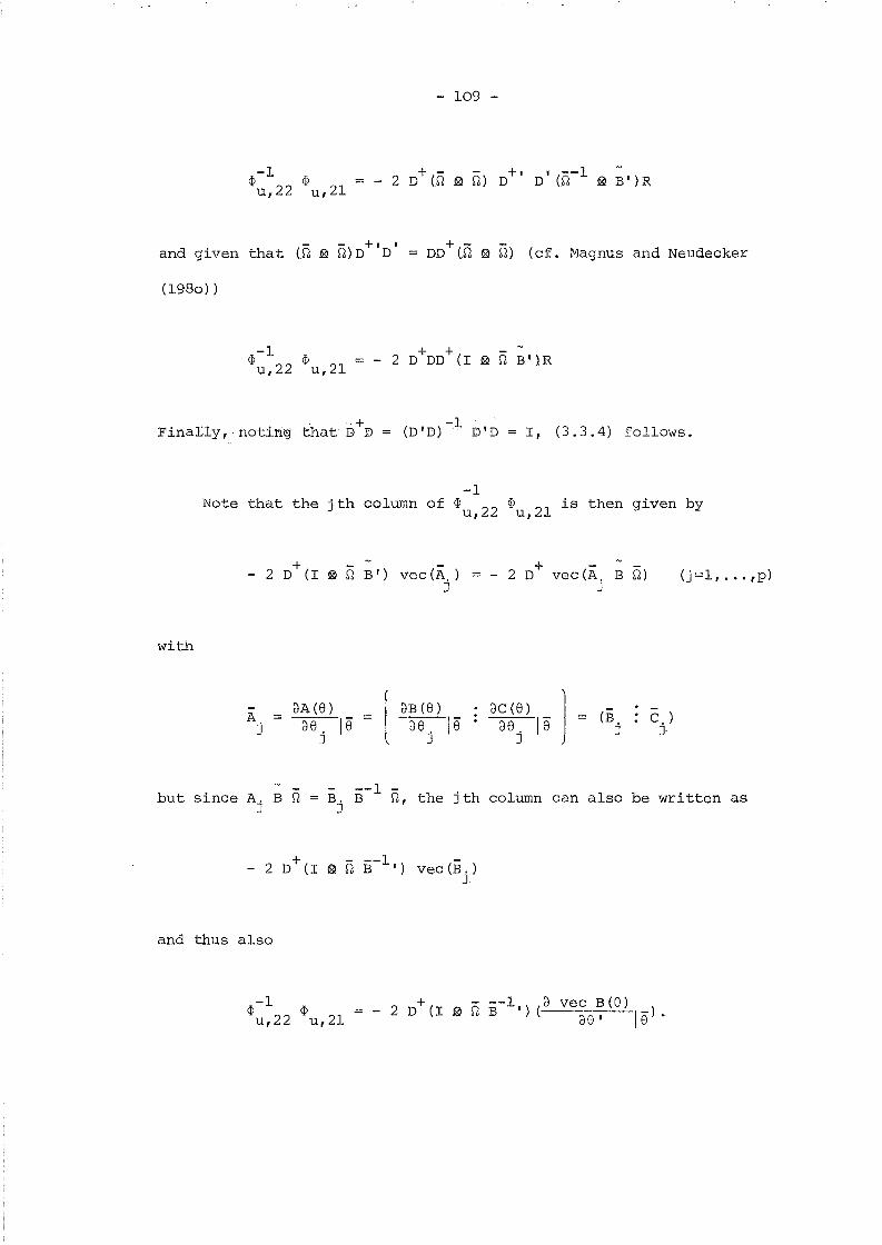
<jJ-l <jJu,22 u,21

- 109 -

+ - - +, I --1- 2 D (Q 0 &i) D D (Q ~ B')R

- - +, I

and given that W ~ &i) D D

(1980) )

DD+(n ~ n) (cf. Magnus and Neudecker

<jJ-l <pu,22 u,21

+ -1·FinaIly, notil1i3 that DD'" (D'D) .. D'D I, (3.3.4) follows.

-1Note that the jth column of <jJ <jJ is then given by

u,22 u,21

with

- 2 D+ vec(A, B &i)J

-A

j

dA(S)

dS, leJ

dB(S)

dS, leJ

• dC(S) ]de. le

J

(8j

C. )J

but since A. B &iJ

- --1B. B &i, the jth column can also be written as

J

and thus also

<jJ-l <pu,22 u,21

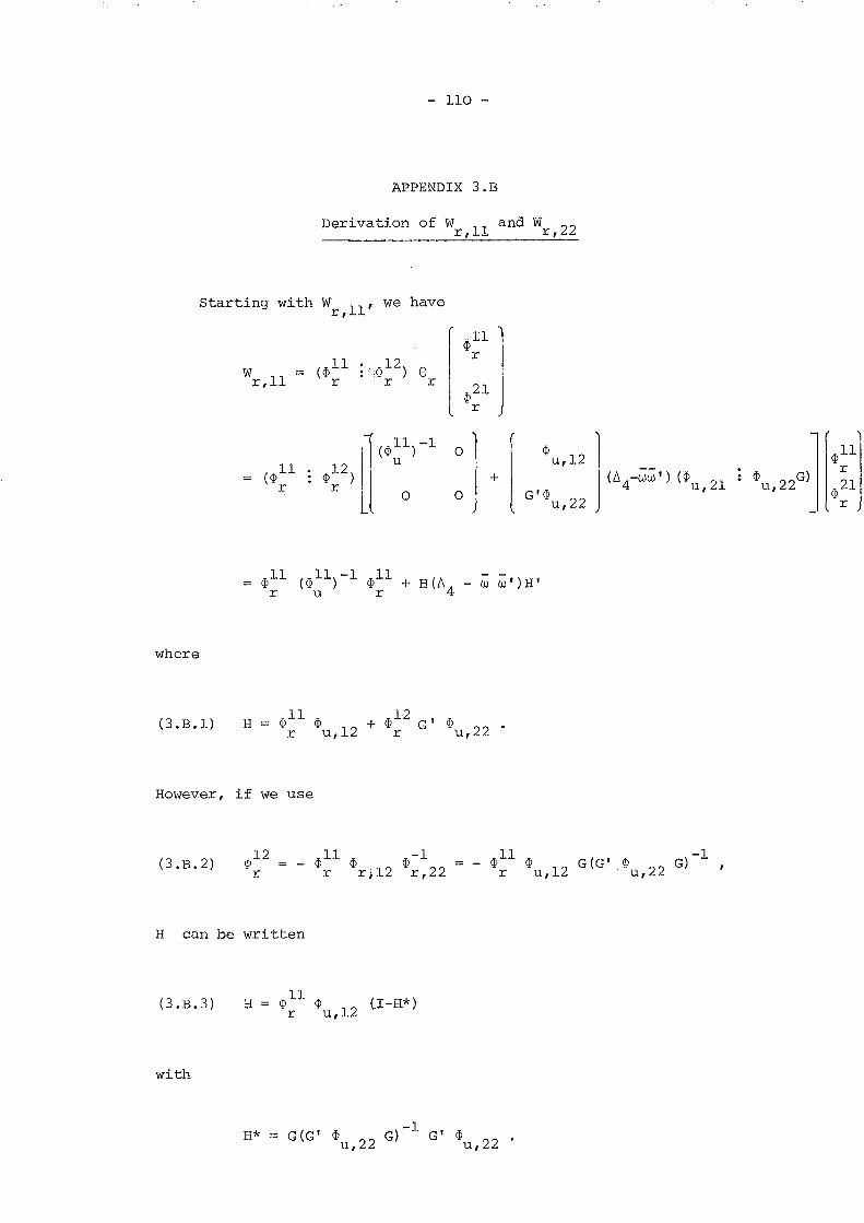
- 110 -

APPENDIX 3.B

Derivation of Wr ,11 and Wr ,22

Starting with Wr ,ll' we have

r<pH

(<P11 : !<p 12)

rWr,11

8r r r

l ;I:>21rr(0~1)-1 1

(

1OU'22

GJ')

0 <pu,12 .~lJ

(<P11

012

) lJ

+ J (L.I 4-ww') (<pu , 21<p

21r r 0 0 G'<Pu,22 r

where

(3.B.1) H <p 11 <p + <p12 G I <p

r u,12 r u,22

However, if we use

(3.B.2) <p 12r

<p ll <p <p-1r r}12 r,22

<p 11 <p G(G' <p G)-l ,r u,12 u,22

H can be written

(3.B.3)

with

H

H*

<p 11 <p CI-H*)r u,12

G(G' <p G)-l G' <pu,22 u,22

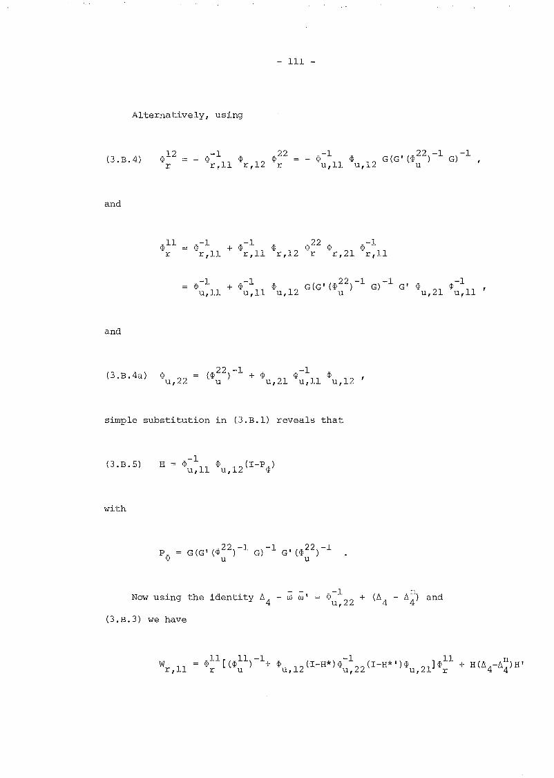
- 111 -

Alternatively, using

(3.B.4)

and

ep-l ep G(G' (ep22)-1 G)-l ,u,ll u,12 u

and

ep-l ep-l ep ep22 ep ep-l11 + r,ll 12 21 11r, r, r r, r,

ep-l ep-l ep G(G' (~22)-1 G)-l G' ep ep-l11 + u,ll 12 21 11u, u, u u, u!,

(3.B.4a) epu,22

(ep 2 2) -1 + ep ep -1 epu u,21 u,ll u,12

simple substitution in (3.B.l) reveals that

(3.B.5)

with

H

Now using the identity ~4 - w w'

(3.B.3) we have

ep-l + (~ _ ~n) andu,22 4 4

Wr,ll

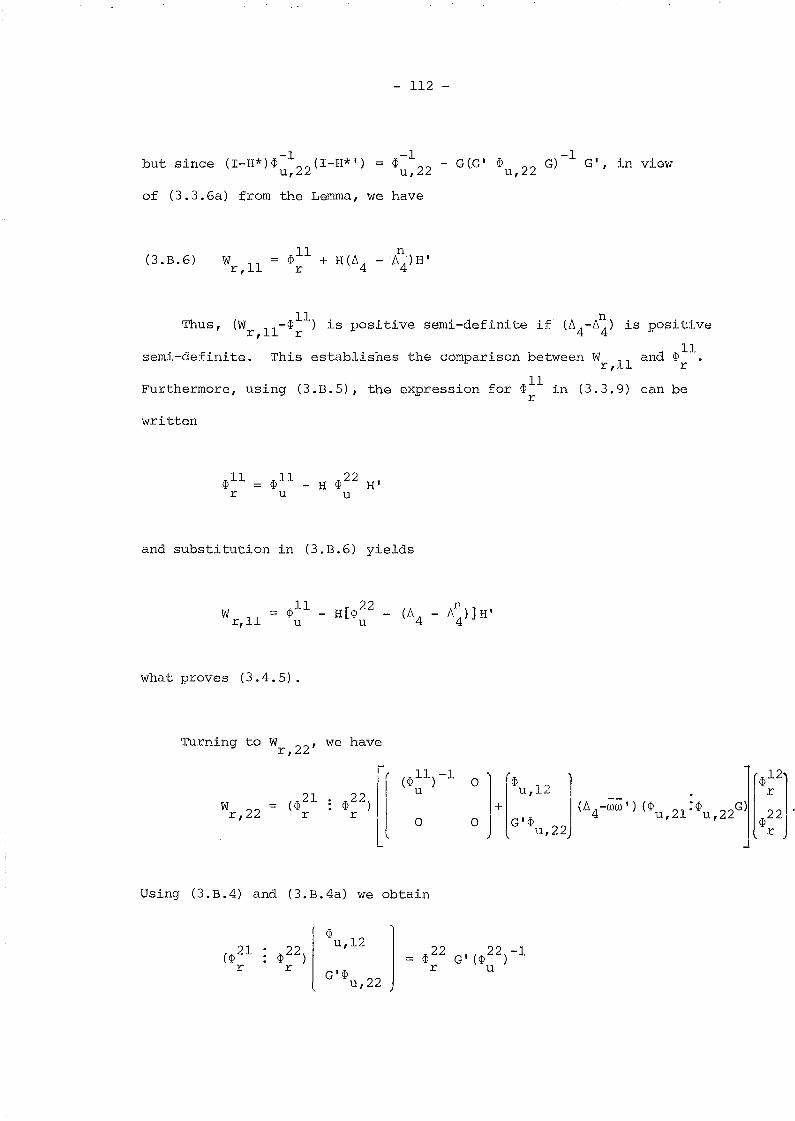
but since (I_H*)~-l (I-H*')u,22

- 112 -

-1 1~ - G(G' ~ G)- G', in viewu,22 u,22

of (3.3.6a) from the Lemma, we have

(3.B.6) Wr,ll

Thus, (Wr,l1-~~l) is positive semi-definite if (L'l4-~) is positive

semi-definite. This establishes the comparison between Wr,ll and ~~l.

Furthermore, using (3.B.5), the expression for ~ll in (3.3.9) can ber

written

~ll ~ll _ H ~22 H'r u u

and substitution in (3.B.6) yields

Wr,ll~ll

u

what proves (3.4.5).

Turning to Wr ,22' we have

If (~11) -1 0

1{U"2 ](;4-ww' Ho 21:. 22GW~J(~21u

Wr,22 .~2) lr

0 0 J G'~ u, u, ~ Ju,22 r

J

Using (3. B. 4) and (3. B. 4a) we obtain

(~21r

~ ]u,12

G'~u,22 =

~22 G' (~22)-1r u

- 113 -

Thus,

Wr,22

Again, using the identity LJ.4 - ww· = .p:~22 + (LJ. 4 - LJ.~) and noting that

from (3.B.4) we obtain

.p12r

we have

Wr,22

.p22 G' (.p22)-1[.p21(.pll)-1 .p12 + .p-l ] (.p22)-1 G .p22r u u u u u,22 u r

+ .p22 G' (.p22)-1(LJ. _ LJ.n) (.p22)-1 G .p22r u 4 4 u r

but .p22 .p21 (.p11)-1 .p12 -1and .p22 [G' (.p22) -lG]-lsince + .pu,22u u u u r u '

this simplifies to

Wr,22

what proves (3.4.6). Alternatively, writing

Wr,22

In view of (3.4.3), (3.4.6a) is also proven.

- 114 -

CMP~R4

WALD AND QUASI-LIKELIHOOD RATIO TESTS OF RANDOM EFFECTS

SPECIFICATIONS IN DYNAMIC MODELS

4.1 Introduction

This Chapter examines, in a quasi-maximum likelihood framework,

the problem of testing covariance restrictions arising from various

random effects specifications. We concentrate on dynamic models with

unrestricted initial observations errors of the type c considered in

Chapter 2. The availability of both ~-restricted and ~-unrestricted

QML estimates suggests the use of straightforward quasi-likelihood

ratio statistics. On the other hand, in cases where explicit expressions

for the constraint equations are available, Wald tests can also be used

as they only require the estimation of the ~-unconstrainedmodel.

Nevertheless, as first pointed out by Box (1953), if the fourth order

moments deviate from their gaussian values, the asymptotic size of tests

on variances that are based on the assumption of normality will be in­

correct. In our context, this has been made clear by the results of

Chapter 3, which show the dependence of the asymptotic distribution of

QML estimates of variance matrices on the value of the actual fourth

order moments of the errors.

Therefore, we start in Section 4.2 by specialising our previous

results to compute the limiting distribution of Qunrestricted for panel

data models. Section 4.3 discusses a Wald test which is robust to the

non-normality of the errors, and shows that appropriate asymptotic

probability limits can still be calculated for the quasi-LR and the

- 115 -

•normal-'Wald I tests when the errOrS are non-normal. In Section 4.4

a limited simulation is carried out in order to investigate how far

the diagnostics from the proposed tests statistics are likely to be

affected by the kurtosis measure of the errors being large compared to

that of the normal distribution. Finally, in Section 4.5 we use the

Michigan Panel to estimate an empirical earnings function for the US

with serially correlated transitory errors. The final specification

we choose is not rejected against the unrestricted model on the basis

of formal tests statistics. In this case, controlling for non-normality

of the errors is crucial as evidence is found that the distribution of

earnings errors has long tails.

4.2 The AVM of ~-Unrestricted QML Estimators for Panel Data

We begin by examining the variances of ~-unrestricted estimators of

the model developed in Chapter 2. Thus

(4.2.1)

(4.2.2)

ll ' z*. + U1 io

ay + Q' + 'z +i(t-l) ~ x it Y i u it(t=l, ... ,T)

E (u . u ~) = rz,1 1

E(u~u~'l = $4*,1 1

and E (u . u ~) = w 1.•10 1 0

Let

w* = \! (Q*) he the !z (T+l) (T+2) vector of variances and covariances

containing the lower triangle of ~*, and letA ...... 1\

El I = Cll I is I )

U U U

A

and w* be

the Q-unrestricted QML estimators of e andw* (Le. 8 maximises (2.4.2».u

A

Following the discussion in Chapter 3, the AVM of e is given by (3.3.1)u

irrespective of non-normality. In this case the coefficient derivative

matrix R is given by

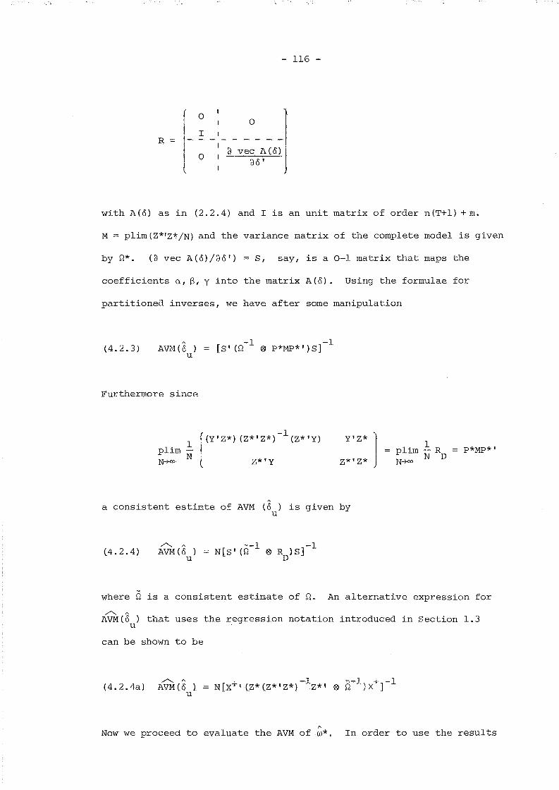
R

o

I

o

- 116 -

o

a vec Aeo)dO'

with A(o) as in (2.2.4) and I is an unit matrix of order n(T+l) +m.

M = plim(Z*'Z*/N) and the variance matrix of the complete model is given

by st*. (d vec A(0)/80') = S, say, is a 0-1 matrix that maps the

coefficients a, S, y into the matrix A(o). Using the formulae for

partitioned inverses, we have after some manipulation

(4.2.3)A

AVM (0 )u

-1 -1[S' W ® P*MP*')S]

Furthermore since

1plim NN-7<>O [

-1(Y'Z*) (Z*'Z*) (Z*'Y)

Z*'Y

Y'Z* ]

Z*'Z*

. 1pllm - RN-7<>O N D

P*MP*'

A

a consistent estimte of AVM (0 ) is given byu

(4.2.4)/'-.. A

AVM (0 )u

where st is a consistent estimate of st. An alternative expression for

/'" A

AVM(o ) that uses the regression notation introduced in Section 1.3u

can be shown to be

/'-.. A

(4.2.4a) AVM(a)u

!'I

Now we proceed to evaluate the AVM of w*. In order to use the results

- 117 -

in Chapter 3 we can either assume that the third order moments are

zero or, alternatively, we may think of the variables in equation (4.2.2)

as being expressed in deviations from cross-section means. Nevertheless,

this assumes that the original model has time specific intercepts (Le.,

if Y is the intercept for period t, this formulation does not enforceOt

the constraints YOl

= ... = YOT which rules out the possibility of

estimating the effect of particular individual-invariant variables).l

A

Using (3.3.3) and (3.4.3), the AVM of w* is given by

(4.2.5) www

A

HoAVM(8 )H' + & - w*w*'u 4

where, in view of (3.3.4), H is given by

H -2D+(I 0 g*B,-l) a vec B(a)

a8'

However since B only depends on a, all columns of H are zero except the

corresponding to the partial derivatives with respect to a. Let us

introduce the following (T+l)x (T+l) matrix

Ba

o

1

o

o

o

o

1

o

o

o

o

o

o

o

o

1

o

o

o

o

then the non-zero column of H is given by

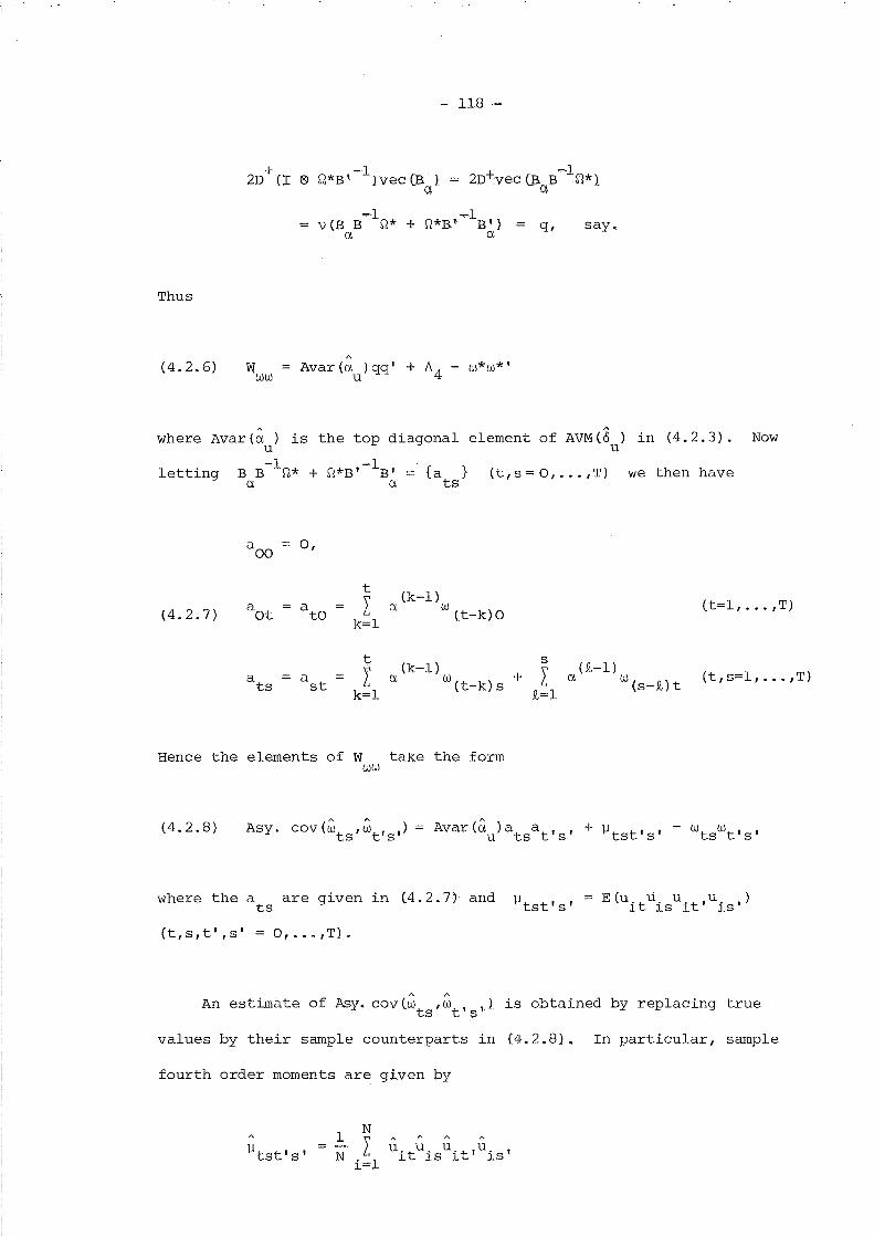
- 118-

+ ~ + ~2D cr @ ~*B' lvec CB. ) = 2Dvec (B B~*)0\ - q, -

Thus

(4.2.6) www

~l ~lv(B B Q* + Q*B' B'}

a a

"AvarCau)qq' + ~4 - w*w*'

CI, say.

"where Avar(a ) isu-1

letting B B Q*a

"-

the top diagonal element of AVMCo ) in (4.2.3).u

{a } (t , s = 0, ... , T) we then havets

Now

aoo 0,

tCk-l)

(4.2.7) aot

atO I a W (t-k)O (t=l, ... ,T)

k=l

t(k-l)

s (9,-1 )a a ! a W + I 0\ W (t,s=l, ... ,T)ts st

k=l(t-k)s 9,=1

(s-9,) t

Hence the elements of W take the formWw

(4.2.8) Asy. cov (Wts ' Wt,s') Avar(a)a a , , + ~ - w wu ts t s tst's' ts t's'

where the a are given in C4.2.7} and ~ts tst's'

Ct,s,t',s' =O, ••• ,T).

" (',

An estimate of Asy. covCWt

,Wt

, ,) is obtained by replacing trues s·

values by their sample counterparts in (4.2.8). In particular, sample

fourth order moments are given by

~tst's'1 ~ ,,(',- L u. u. u.t,u. ,N . 1 ~t lS 1 lS

1=

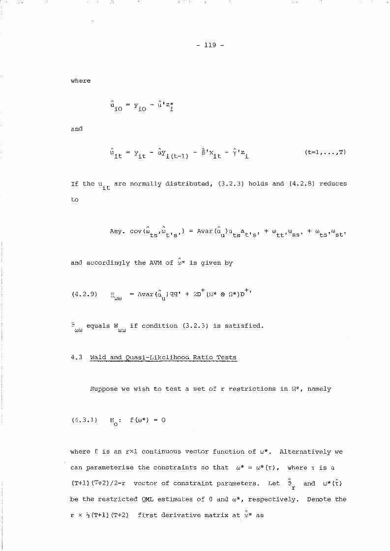
- 119 -

where

and

Y - ay - S'x - yA,Z.it i(t-l) it 1

(t=l, ... ,T)

If the uit

are normally distributed, (3.2.3) holds and (4.2.8) reduces

to

A A

Asy. cov(w ,Wt

, ,)ts s

A

Avar(a)a at' , + 00 00 + 00 00u ts s tt' ss' ts' st'

and accordingly the AVM of w~ is given by

(4.2.9)~ww

A + +Avar(a )qq' + 2D (~* 0 ~*)D I

u

equals W if condition (3.2.3) is satisfied.woo woo

4.3 Wald and Quasi-Likelihood Ratio Tests

Suppose we wish to test a set of r restrictions in ~*, namely

(4.3.1) H: f(w~)o

o

where f is an rxl continuous vector function of 00*. Alternatively we

can parameterise the constraints so that 00* = W*(T), where T is a

(T+l) (T+2) j2-r vector of constraint parameters.A

Let e and w*(~}r

be the restricted QML estimates of e and 00*, respectively. Denote the

A

r x ~(T+l) (T+2) first derivative matrix at w~ as

F

- 120 -

af CW~L

aW*'l "w*

Let Www

andWW

be consistent estimates of Www

and ~ ,ww

respectively.

Then we introduce the three following statistics

(4.3.2) WT

(4.3.3) NWT

(4.3.4) QLR

A A -1 A

Nf(w*)'(FW F ' ) f(W"'),ww

" A -1"NfCw*)' (FS F ' ) f(w*)ww '

A A A A

2[LCe ,w*) - L(e ,W*(T»].u r

WT is a robust Wald criterion of the type discussed by White (1982) and

on the null hypothesis it is distributed asymptotically as a X2 with r

degrees of freedom. NWT, henceforth 'Normal-Wald', is an appropriate

Wald criterion on the assumption of normality of the error term. Specifi-

cally, in addition that all constraints are satisfied, NWT also requires

that condition C3.2.3) is true in order to be distributed asymptotically

as a X2 • Furthermore, since the quasi-likelihood ratio statistic has

the same asymptotic distribution as NWT under the null hypothesis,

similar remarks apply to the statistic QLR. 2

"However, if the matrices Wand F are available we still can computeww

the asymptotic distribution of the QLR and NWT statistics under the null

hypothesis. To show this, note that if the restrictions are satisfied

we may define a standardised rxl random vector c such that

(4.3.5)

- 121 -

moreover, let us define the r~r matrix

(4.3.6)

so that

(4.3.7) NWT

~ ~ ~ -l ~ ~(FW F ') (F s: F I ) (FW F I )

WW ww ww

c''¥c

The canonical form of \jI is given by \jI = LAL', where A is a diagonal matrix

containing the latent roots of \jI and L is an orthogonal matrix. Because

of L'L = I, the elements of the transformed vector c+ = L'c still are

standard normal random variables in the limit. Therefore

(4.3.8) NWT

Hence the asymptotic distribution of NWT is a linear combination of

independent X2 variables with one degree of freedom and so is the asymp-

totic distribution of the quasi-likelihood ratio test, which can be

evaluated numerically from the central Imhof computing procedure (see

Imhof (1961) and Koerts and Abrahamse (1969)). The weights are given

by the latent roots of~ ~ -1

(FW F ' ) (FS: F ' ) which is a similar matrixww WW·

to \jI Cc£. Foutz and Srivastava (1977) and MaCurdy (1981)).

Summing up, likelihood ratio tests of covariance restrictions

crucially depend on the assumption of normality of the error term for

being asymptotically distributed as a X2 under the null hypothesis,

unlike the case of regression parameter restrictions. For practical

purposes, this means that in order to obtain a Wald or an LR test of

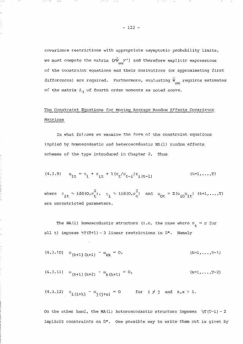
- 122 -

covariance restri.ctions with appropriate asymptotic probability limits,

we must compute the matrix (FW F' 1 and therefore explicit expressionsww

of the constraint equations and their derivatives (or approximating first

differences) are required.A

Furthermore, evaluating W requires estimatesww

of the matrix &1 of fourth order moments as noted above.

The Constraint Equations for Moving Average Random Effects Covariance

Matrices

In what fol~ows we examine the form of the constraint equations

implied by homoscedastic and heteroscedastic MA (l) random effects

schemes of the type introduced in Chapter 2. Thus

(4.3.9) (t=l, ... ,T)

where and

are unrestricted parameters.

The MA(l) homoscedastic structure (i.e. the case where 0t

all t) imposes ~T(T+l) - 3 linear restrictions in Q*. Namely

o for

(4.3.10) W(k+l) (k+l) - wkk0, (k=l, ••. , T-l)

(4.3.11) W(k+l) (k+2) - wk (k+l) 0, (k=1 , . . . , T- 2 )

(4.3.12) o for i ~ j and k,s > 1.

On the other hand, the MA (1) heteroscedastic structure imposes ~T (T-l) - 2

implicit constraints on Q*. One possible way to write< them out is given by

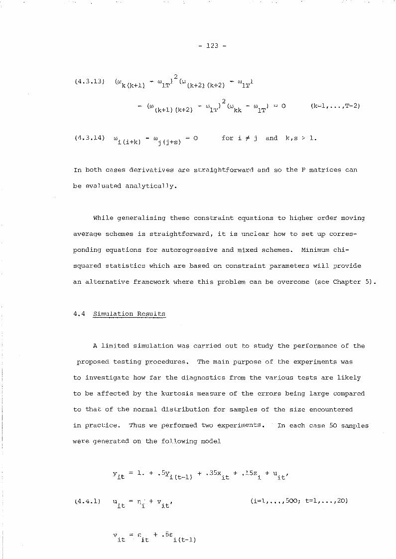
(4.3.13 )

- 123 -

2lWk Ck+U - wlT ) Lw (k+2J(k+2) ~ wlT )

2- (W tk+l) (k+2) - wlT ) (Wkk - wlT ) o (k=l, ... ,T-2)

(4.3.14) o for i ~ j and k,s > 1.

In both cases derivatives are straightforward and so the F matrices can

be evaluated analytically.

While generalising these constraint equations to higher order moving

average schemes is straightforward, it is unclear how to set up corres-

ponding equations for autoregressive and mixed schemes. Minimum chi-

squared statistics which are based on constraint parameters will provide

an alternative framework where this problem can be overcome (see Chapter 5).

4.4 Simulation Results

A limited simulation was carried out to study the performance of the

proposed testing procedures. The main purpose of the experiments was

to investigate how far the diagnostics from the various tests are likely

to be affected by the kurtosis measure of the errors being large compared

to that of the normal distribution for samples of the size encountered

in practice. Thus we performed two experiments.

were generated on the following model

In each case 50 samples

(4.4.1)

V 8 + .58it it i(t-l)

Ci=l, ••• ,500; t=l, ..• ,20)

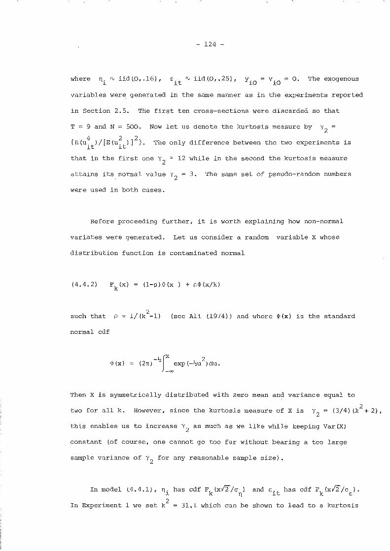
- 124 -

where ni

rv iid(O,.l61, Eit

rv iidCO,.251, YiO

= via = O. The exogenous

variables were generated in the same manner as in the experiments reported

in Section 2.5. The first ten cross-sections were discarded so that

T = 9 and N = 500. Now let us denote the kurtosis measure by y =2

4 2 2{E (u

it) / [E (u

it)] }. The only difference between the two experiments is

that in the first one Y2 ~ 12 while in the second the kurtosis measure

attains its normal value Y2

were used in both cases.

3. The same set of pseudo-random numbers

Before proceeding further, it is worth explaining how non-normal

variates were generated. Let us consider a random variable X whose

distribution function is contaminated normal

(4.4.2) Fk(X) (l-p)~(x ) + p~(x/k)

such that P

normal cdf

(see Ali (1974» and where ~(x) is the standard

~(x)1 JX 2-'2

(2TI) _ooexp(-~u )du.

Then X is symmetrically distributed with zero mean and variance equal to

two for all k. However, since the kurtosis measure of X is Y2

= (3/4) (k2

+ 2),

this enables us to increase Y2

as much as we like while keeping Var(X)

constant (of course, one cannot go too far without bearing a too large

sample variance of Y2

for any reasonable sample size).

In model (4.4.1), ni

has cdf Fk

(xl2/ern) and Eit

has cdf Fk

(xn/ers)'

In Experiment 1 we set k2

= :31.1 which can be shown to lead to a kurtosis

- 125 -

measure for u. of about twelve. In Experiment 2, k2

is simply set tolt

two.

For each replication both restricted and unrestricted QML estimates

were obtained and, from those, QLR, NWT and WT tests of the restrictions

(4.3.10) to (4.3.12) were calculated. Finally, the Imhof routine was

used to compute proper asymptotic limits for the QLR and the NWT statistics.3

Tables 1 and 2 summarise the results. WT appears to be slightly upward

biased (Le. too rejecting) especially in Experiment 2, while NWT shows a

smaller bias in the opposite direction. QLR lies in between and so it

seems to be the best option, at least in our example. However, the out-

standing feature of these results is the confirmation of the fact that in

practice tests of covariance matrix restrictions are useless without

controlling for departures of the errors from normality: when the dis-

tribution of the errors is long-tailed, the mean and the variance of the

QLR test under the null hypothesis are far greater than their X2 counter-

parts (in our case, the mean is 42 and the variance 84).

4.5 Estimation of Earnings Functions for the US

The purpose of this Section is to estimate empirical earnings

functions for panel data that take into account the dynamic features of

the sample under consideration. We wish to choose a specification that

is not rejected against a reasonably general maintained hypothesis on

the basis of formal test statistics. A standard earnings function is

best interpreted as a reduced form relation made up of a mixture of

several supply and demand factors, among which personal characteristics,

like years of education and work experience, play the central role. This

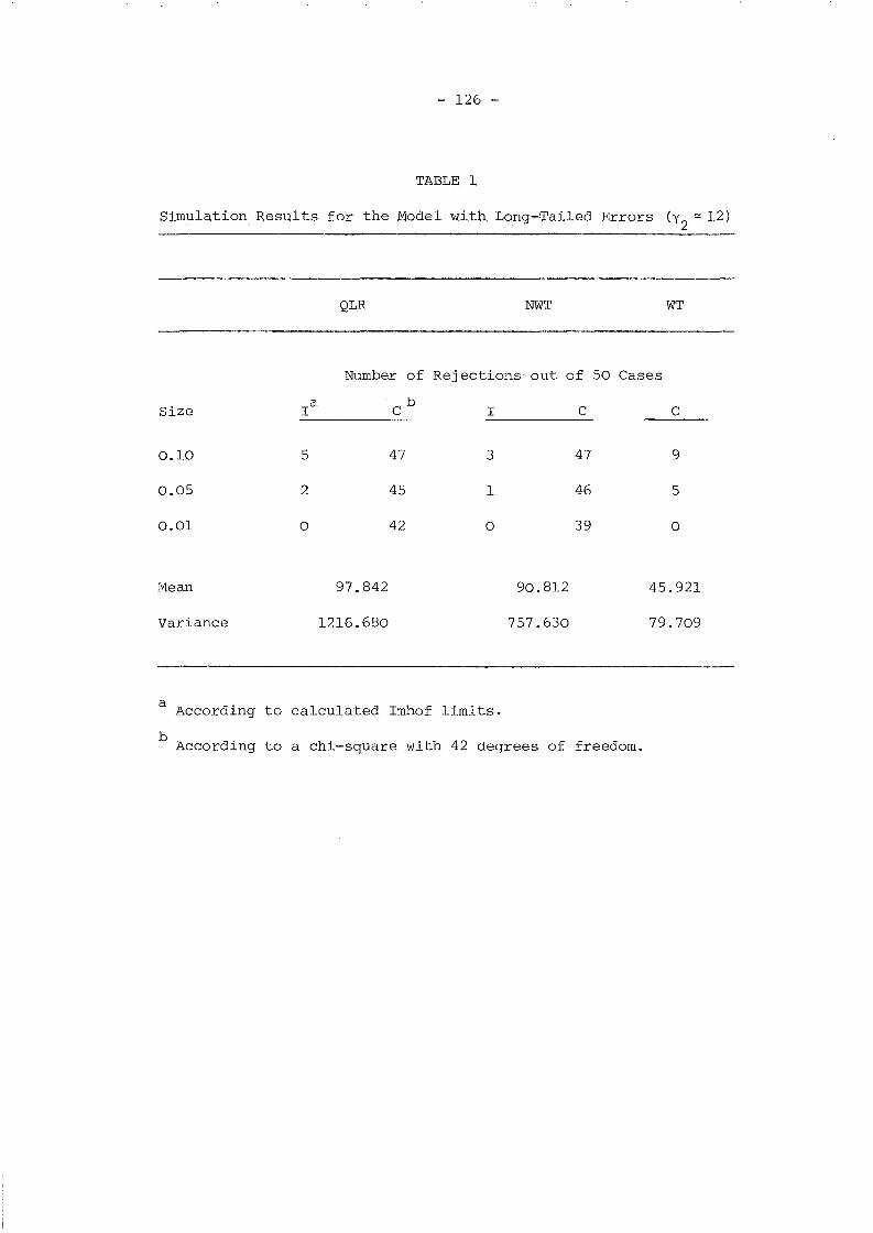
- 126 -

TABLE 1

Simulation Results for the Model wi th Long~Tai1ed Errors er2 '" 12)

QLR NWT WT

Number of Rejections out of 50 Cases

Size la cb I C C

0.10 5 47 3 47 9

0.05 2 45 1 46 5

0.01 0 42 0 39 0

Mean

Variance

97.842

1216.680

90.812

757.630

45.921

79.709

aAccording to calculated lmhof limits.

bAccording to a chi-square with 42 degrees of freedom.

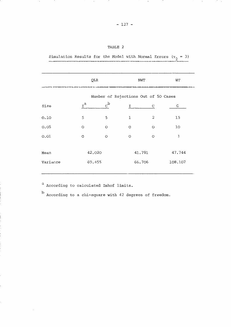
- 127 -

TABLE 2

Simulation Results for the Model with Normal Errors (Y2 3)

QLR NWT WT

Number of Rejections Out of 50 Cases

Ia b

Size C I C C

0.10 5 5 1 2 15

0.05 0 0 0 0 10

0.01 0 0 0 0 1

Mean

Variance

42.020

69.455

41.791

66.706

47.744

108.107

aAccording to calculated Imhof limits.

bAccording to a chi-square with 42 degrees of freedom.

- 128 -

means that some caution is required in drawing conclusions from the

estimated coefficients unless we are prepared to think in terms of the

mincerian schooling model.

Our sample corresponds to male heads of households observed through

ten consecutive years (1967-1976) of the Michigan Panel of Income

Dynamics, with the following characteristics: (i) were not included in

the SEO sample since it was non-random, lii) have remained the same over

the sample period (i.e., no split-off family units where the head has

changed), (iii) were not unemployed, retired or full-time students,

(iv) reported positive annual hours and earnings throughout the sample

period. In view of this, we are left with a sample of 742 individuals.

We decided to transform the data into deviations from cross-section

means (i.e., X~t = x t - (l/N)L~ lX't)i this is equivalent to introducing1. i 1.= 1.

a set of time dummies that capture the combined effect of all potential

4macroeconomic explanatory variables llike productivity changes) • Our

dependent variable is the logarithm of the real hourly earnings (in 1967

dollars) and, apart from lagged earnings, we consider some of the explan-

atory variables that are included in the most conventional earnings

functions: years of education, linear and quadratic age effects (note

that Ait

- At = AiO

- AO)' a dummy variaole for non-whites and another

binary variable for the professional and managerial occupational groups.

Given the absence of other measures of work experience in the sample, this

variable is usually defined as the time period that has elapsed since an

individual left school (e.g., Exp = Age - Schooling - 6), but as this

creates an artifical association between experience and schooling, nothing

is lost by using instead the age variable itself, On the other hand,

- 129 -

having an experience variable defined in such a way rules out the pos­

sibility of distinguishing a dynamic response of earnings to changes in

experience from a static one.

Table 3 gives the results of estimates for the model in which Q*

is treated as an unrestricted matrix. Crude instrumental variable

estimates have been used as initial consistent values in order to start

off the iterative procedure for the QML estimator. Asymptotic standard

errors have been calculated using structural form estimates of p* in

(4.2.3). The actual estimates we have found are very similar to the

results in other studies that assume exogenous regressors (e.g., Lillard

and Willis (1978»; using years of education, age, age squared and race

as explanatory variables, we obtain that an additional year of education

leads to a 7.3 per cent higher earnings. However, the introduction of

the occupational dummy (model 2 in Table 3) has the effect of reducing

the mean schooling coefficient to 5.1 per cent while leaving all other

coefficients unchanged.

Turning now to consider constrained models, in Tables 4 and 5 we

present the results for the homoscedastic models, and in Table 6 for the

heteroscedastic ones. In these cases, asymptotic standard errors have

been calculated by using the differencing estimates of the second deriv­

atives of the log-likelihood function, and thus they may be affected by

the non-normality of the errors. The estimated coefficients in the

homoscedastic cases show little variation in relation to those obtained

prior to enforcing the restrictions. The results for the ARMA(l,l)

specifications in Table 4 clearly point to models with moving average

errors, which are presented in Table 5.

- 130 -

When we let the variances of the transitory errors vary over time,

there is an increase in the moving average coefficient while the coef-

ficient of the lagged dependent variable decreases and the derived mean

effects of the independent variables remain fairly unchanged. This

suggests some degree of indetermination in the contribution of the

systematic component, relative to the moving average one, to the overall

time dependencies in the sample (the estimated asymptotic correlation

between the two coefficients is -.85). On the other hand, the estimated

A2ratios Pt' t=1,2, ... ,9, show some variation but there is no evidence of

any systematic pattern. In fact, it should be noticed that, since the

only time-varying explanatory variable we are including in the present

application is a trending one, the model with lagged endogenous variable

and moving average errors is not distinguishable from a static model

with ARMA errors. So, all we can say about the motion of this model is

that a stochastic individual level is determined by the observed charac-

tristics and the unobservable effect n~ = n,/(l-a) once for all before1 1

the start of the sample period; and then, as random shocks come out, the

log-earnings of a particular individual evolve around its random mean

following a serially correlated pattern controlled by a and \. In

particular, we obtain that unobserved permanent differences among in-

'd 1 f 61 f 1 ' . 5divl ua s account or per cent 0 tota error varlatlon.

Now we proceed to test the covariance restrictions implied by our

random effects specifications using the methods developed in Section 4.3.

, 6Table 7 glves the results. Clearly, if we rely on the assumption of

normality of the errors, and so we compare the QLR and the NWT criteria

against X2 limits, both the homoscedastic and the heteroscedastic sets

of constraints are rejected at any reasonable level of significance.

- 131 -

But the si.tuation is the opposite when we look a,t the Wald test and

when QLR or NWT are compared against limits calculated from their appro­

priate asymptotic distribution under the null hypothesis. Clearly, the

constraints for the heteroscedastic model are not rejected and, while

for the homoscedastic moving average scheme WT is somewhat higher than

its expected value of 42, all three tests accept the restrictions at

the 90 per cent level.

The values of the standardised fourth order cumulants of the errors

for the unrestricted model (version 1) are given in Table 8. These

values are rather high and this suggests that the distribution of the

errors is long-tailed. In fact, the shape of the distribution as perceived

by plotting the histogram of the errors is fairly normal. This points

to the fact that QLR and NWT are not X2 variates mainly as a consequence

of long tails in the density of the errors.

- 132 -

TABLE 3

QML Estimates with Unrestricted Covariance Matrix

Dependent Variable: Log Hourly Earningsa

Model 1 Model 2

EstimatesDerived

eMean Effects

EstimatesDerived

Mean Effects

Years of .0112 b .0730 .0099 .0510Education ( .0037) (.0034)

Age .0046 .0301 .0058 .0297(.0030) (.0034)

Age -.000046 -.0003 -.000059 -.0003Squared ( .000031) ( .000035)

c.0213 .1391 .0269 .1384Race

( .0131)

Occupationd

.0469 .2413( .0161)

Lagged .8469 .8057Dependent (.0445) (.0553)Variable

aData in mean deviation form (N= 742, T=9, period 1967-1976).

bStandard errors in parentheses.

cDummy variable: 1 if individual is white.

d Dummy variable: 1 if individual belongs to professional ormanagerial groups in 1967.

e Calculated as Y~ = Yk

/ (1-&) •

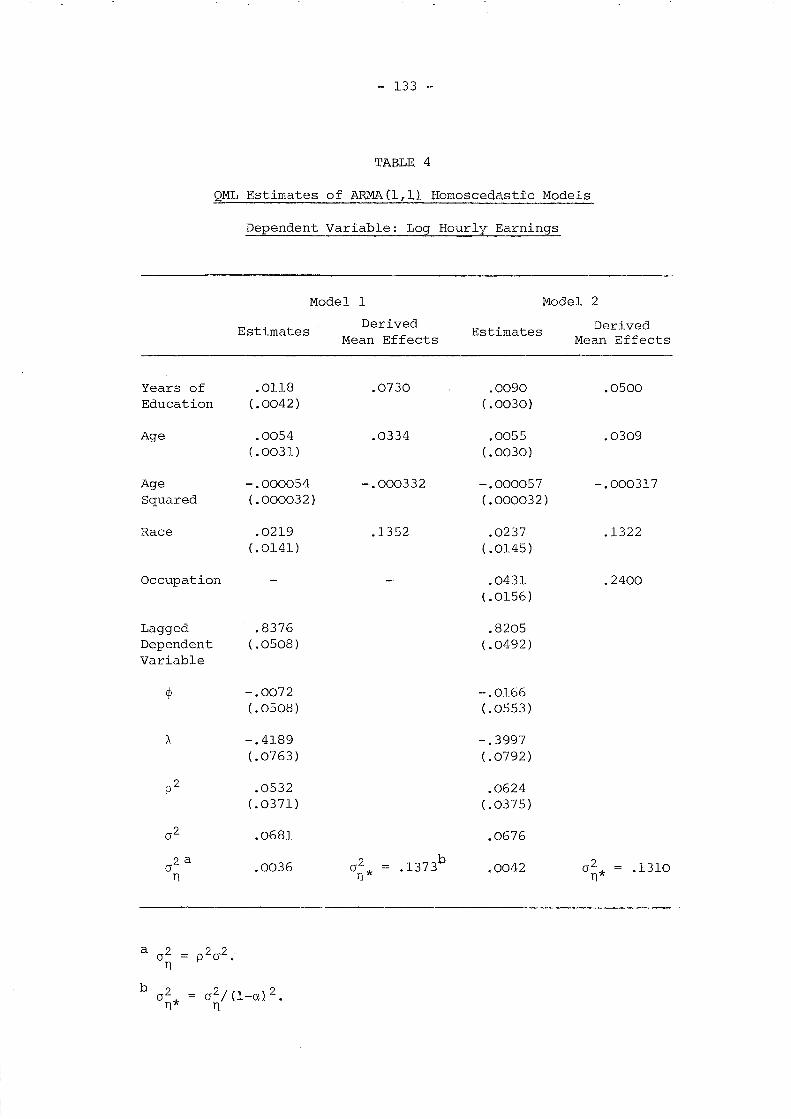
- 133 ..

TABLE 4

QML Estimates of ARMA (1 r U Homoscedastic Models

Dependent Variable: Log Hourly Earnings

Model 1 Model 2

EstimatesDerived

Estimates DerivedMean Effects Mean Effects

Years of .01l8 .0730 .0090 .0500Education ( .0042) (.0030)

Age .0054 .0334 .0055 .0309(.0031) ( .0030)

Age -.000054 -.000332 -.000057 -.000317Squared (.000032) ( .000032)

Race .0219 .1352 .0237 .1322(.0141) (.0145)

Occupation .0431 .2400(.0156)

Lagged .8376 .8205Dependent ( .0508) (.0492)Variable

<P -.0072 -.0166(.0508) (.0553 )

-.4189 -.3997(.0763) (.0792)

p2 .0532 .0624(.0371) (.0375)

0 2 .0681 .0676

2a .0036 0 2 .1373b

.0042 0 2 .13100n n* n*

- 134 -

TABLE 5

QML Estimates of Moving Average Romoscedastic Models

Dependent Variable: Log Hourly Earnings

Model 1 Model 2

EstimatesDerived

EstimatesDerived

Mean Effects Mean Effects

Years of .0116 .0728 .0086 .0498Education (.0036) (.0028)

Age .0053 .0331 .0052 .0304( .0030) (.0028)

Age -.000053 -.000333 -.000054 -.000314Squared ( .000031) ( .000029)

Race .0214 .1345 .0225 .1309(.0137) (.0137 )

Occupation .0413 .2398(.0135)

Lagged .8410 .8279Dependent (.0429) (.0440)Variable

A -.4287 -.4219(.0303 (.0295)

p2 .0511 .0579(.0318) (.0342)

0'2 .0681 .0676

0'2 .0035 0'2 .1378 .0039 0'2 .1322n n* n*

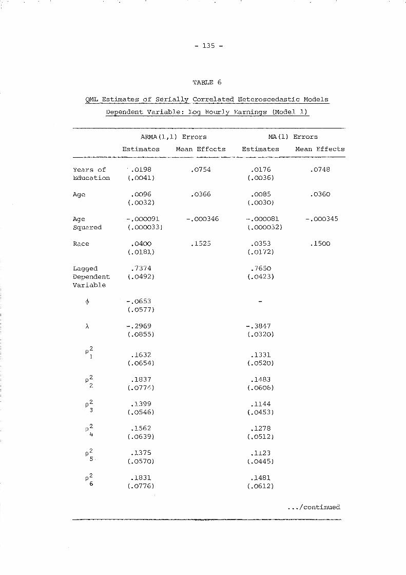
- 135 -

TABLE 6

QML Estimates of Serially Correlated aeteroscedastic Models

Dependent Variable: Log Hourly Earnings (Model 1).

ARMA(l,l) Errors MA(l) Errors

Estimates Mean Effects Estimates Mean Effects

Years of .0198 .0754 .0176 .0748Education ( .0041) ( .0036)

Age .0096 .0366 .0085 .0360(.0032) ( .0030)

Age -.000091 -.000346 -.000081 -.000345Squared ( .000033) ( .000032)

Race .0400 .1525 .0353 .1500(.0181) (.0172 )

Lagged .7374 .7650Dependent (.0492 ) (.0423)Variable

~ -.0653(.0577)

-.2969 -.3847( .0855) ( .0320)

p2.1632 .13311

(.0654) (.0520)

p2 .1837 .14832 ( .0774) ( .0606)

p2 .1399 .11443 (.0546) (.0453 )

p2 .1562 .12784 (.0639) (.0512)

p2 .1375 .11235 (.0570) (.0445)

p2 .1831 .14816 (.0776) (.0612)

••• /continued

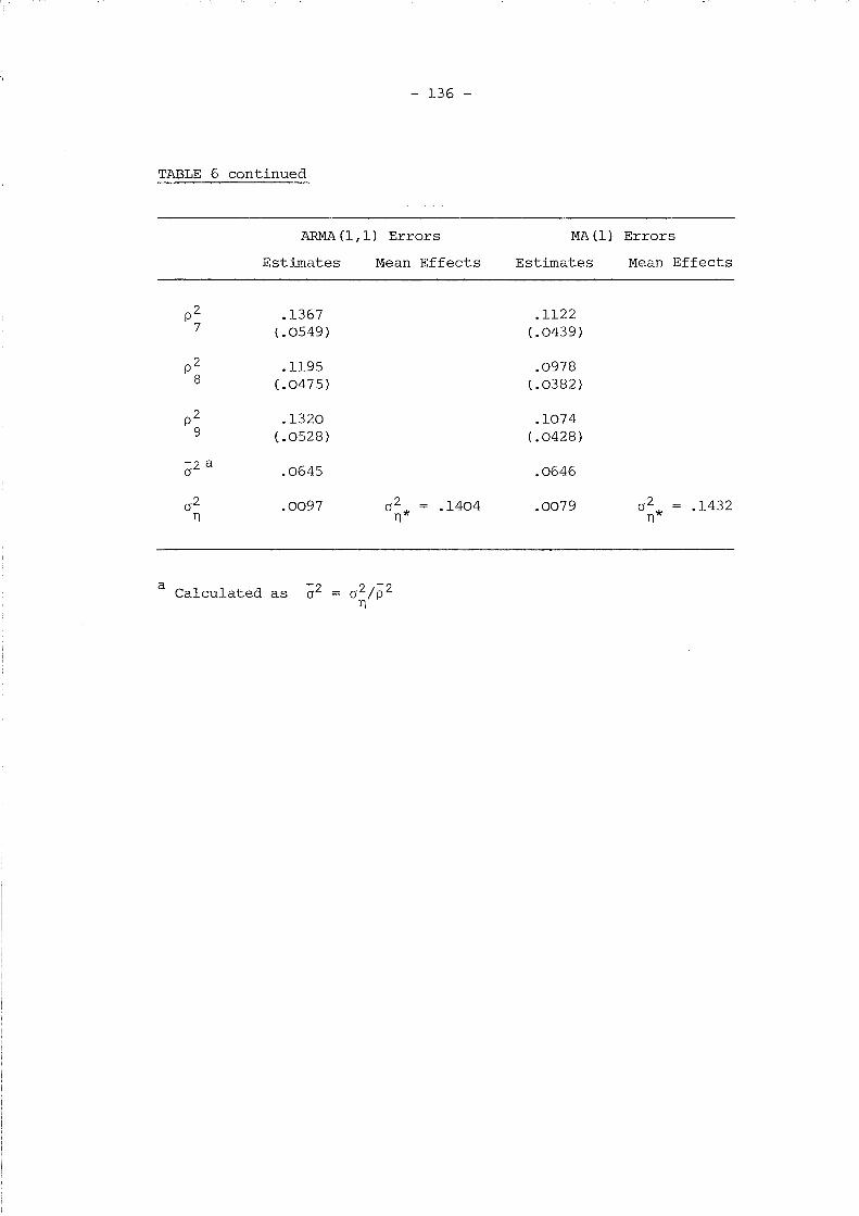
TABLE 6 continued

- 136 -

ARMA (1,1) Errors MA (1) Errors

Estimates Mean Effects Estimates Mean Effects

p2 .1367 .11227 (.0549) (.0439)

p2 .1195 .09788 (.0475) ( .0382)

p2 .1320 .10749 (.0528) (.0428)

0:2 a .0645 .0646

02 .0097 0 2 .1404 .0079 0

2 .143211 11* 11*

a Calculated as 0:2

- 137 -

TABLE 7

Asymptotic Tests of Random Effects Constraints (Model l)

Criteria x2

Prob. LimitImhof

Prob. Limit

Heteroscedastic Moving Average Scheme (D.F.=34)

Likelihood Ratio

Normal-Wald

Wald

82.7

80.8

32.1

1.00

1.00

0.44

<0.57

0.53

Homoscedastic Moving Average Scheme (D.F.=42)

Likelihood Ratio

Normal-Wald

Wald

138.5

142.5

51. 5

1.00

1.00

0.85

<0.78

0.79

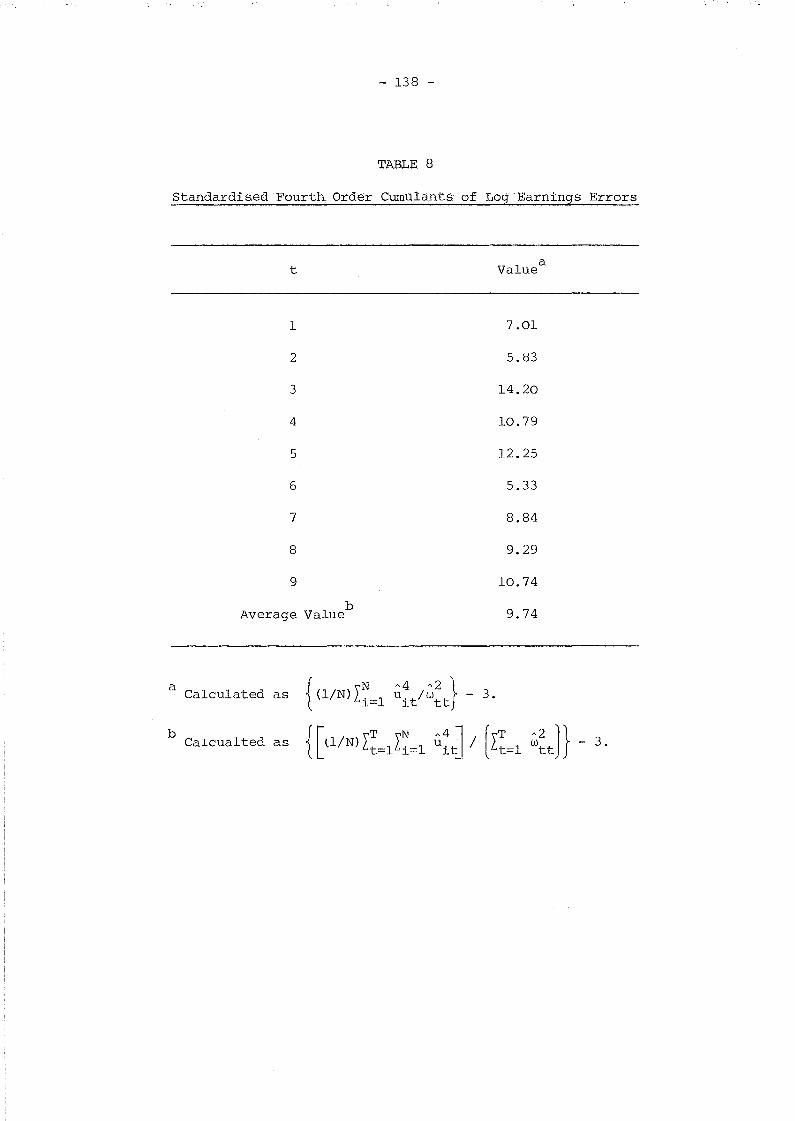
- 138 -

TABLE 8

Standardised Fourth Order Curnulants of LoSj" Earnings Errors

t Valuea

1 7.01

2 5. en

3 14.20

4 10.79

5 12.25

6 5.33

7 8.84

8 9.29

9 10.74

Average Valueb

9.74

a Calculated as

bCalcualted as

{ \N ~4 ~2}. (l/N) L. 1 u. tl W - 3.

l= l tt

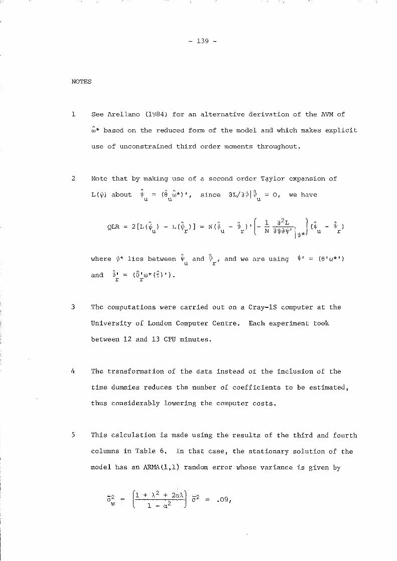
- 139 -

NOTES

1 See Arellano (1~84) for an alternative derivation of the AVM of

w* based on the reduced form of the model and which makes explicit

use of unconstrained third order moments throughout.

2 Note that by making use of a second order T~ylor expansion of

A

L(1jJ) about 1jJu (8 ~*)', since 3L/31)Jlw = 0, we haveu u

QLR 2 [1. (~ )u

1. C~ )]r

A

N(1jJu

where 1jJ* lies between ~ and ~ , and we are using 1jJ'u r

(8'w*')

and ~,r

(8'w*cT)').r

3 The computations were carried out on a Cray-lS computer at the

University of London Computer Centre. Each experiment took

between 12 and 13 CPU minutes.

4 The transformation of the data instead of the inclusion of the

time dummies reduces the number of coefficients to be estimated,

thus considerably lowering the computer costs.

5 This calculation is made using the results of the third and fourth

columns in Table 6. In that case, the stationary solution of the

model has an ARMA(l,l} random error whose variance is given by

.09,

- 140 -

therefore, total error variance for the stationary solution is

02 + a:2 .23.n* w

6 These results correspond to the model that excludes the occu-

pational dummy, but the inclusion of this variable leaves the

value of the test criteria almost unchanged.

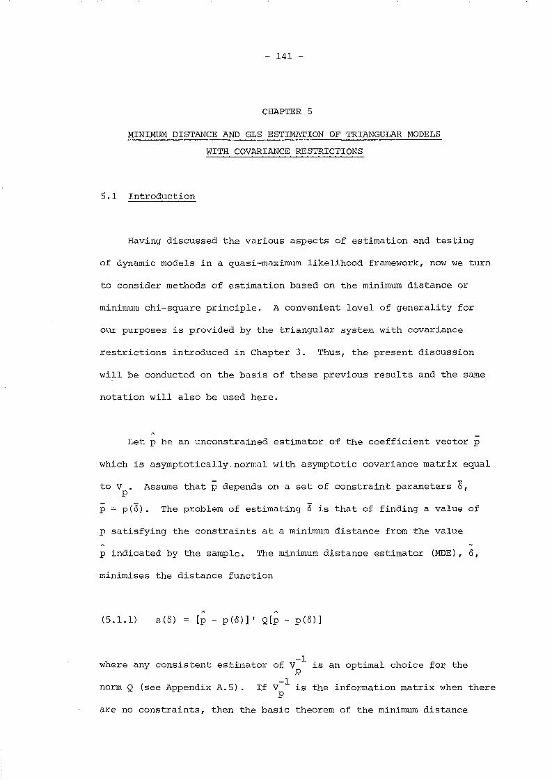
- 141 -

CHAPTER 5

MINIMUM DISTANCE AND GLS ESTIMATION OF TRIANGULAR MODELS

WITHCOVARIANCE RESTRICTIONS

5.1 Introduction

Having discussed the various aspects of estimation and testing

of dynamic models in a quasi-maximum likelihood framework, now we turn

to consider methods of estimation based on the minimum distance or

minimum chi-square principle. A convenient level of generality for

our purposes is provided by the triangular system with covariance

restrictions introduced in Chapter 3. Thus, the present discussion

will be conducted on the basis of these previous results and the same

notation will also be used here.

Let p be an unconstrained estimator of the coefficient vector p

which is asymptotically normal with asymptotic covariance matrix equal

Assume that p depends on a set of constraint parameters 8,to V .P

P = p(8). The problem of estimating 8 is that of finding a value of

p satisfying the constraints at a minimum distance from the value

p indicated by the sample. The minimum distance estimator (MDE), 0,

minimises the distance function

(5.1.1) s (0) [p - p(o)] I Q[p - p(o)]

-1where any consistent estimator of V is an optimal choice ~Qr the

p

norm Q (see Appendix A.5). If V-l

is the information matrix when therep

are no constraints, then the basic theorem of the minimum distance

- 142 -

method establishes that 0 is asymptotically e~ficient and therefore

asymptotically equivalent to the maxim.um likelihood estimator. More

generally, as discussed by Chamberlain (1982), the quasi-maximurq

likelihood estimator has the same limiting distribution as a certain

minimum distance estimator; but in general that minimum distance

estimator is not using the optimal norm. The cases where the AVM of the

unconstrained QML estimator of p remains the Same under non-normality

constitute a relevant exception. We know that this is not the case in

a simultaneous equation model if covariance constraints are available.

Thus, in our model we may expect to obtain estimators of both slope

and covariance parameters that are efficient relative to the QML

estimator by application ofi. the minimum distance method when the errors

are non-normal. Most of the basic discussion of the general principle

is contained in Chiang (1956) and Ferguson (1958). Malinvaud (1970)

considers the minimum distance estimation of multivariate nonlinear

regression models with unrestricted covariance. The non-normal case

and its relation to QML estimators of covariance parameters is discussed

in Chamberlain (1982).

The order of presentation in this Chapter is as follows. Section

5.2 defines the joint MDE of slope and covariance parameters that makes

use of the optimal norm. In Section 5.3 an expression of the AVM of

this estimator is derived which can be used as abound to characterise

efficient estimators. Section 5.4 deals with separate MDE of

covariance parameters based on 3SLS, MD or QML estimates of unrestricted

Q, which are shown to be efficient. Section 5.5 discusses various

generalised least squares estimators of the slope coefficients under

linear constraints, and an efficient GLS estimator robust to non-normality

is presented.l

Finally, Section 5.6 examines the problem of estimating

subsets of equations.

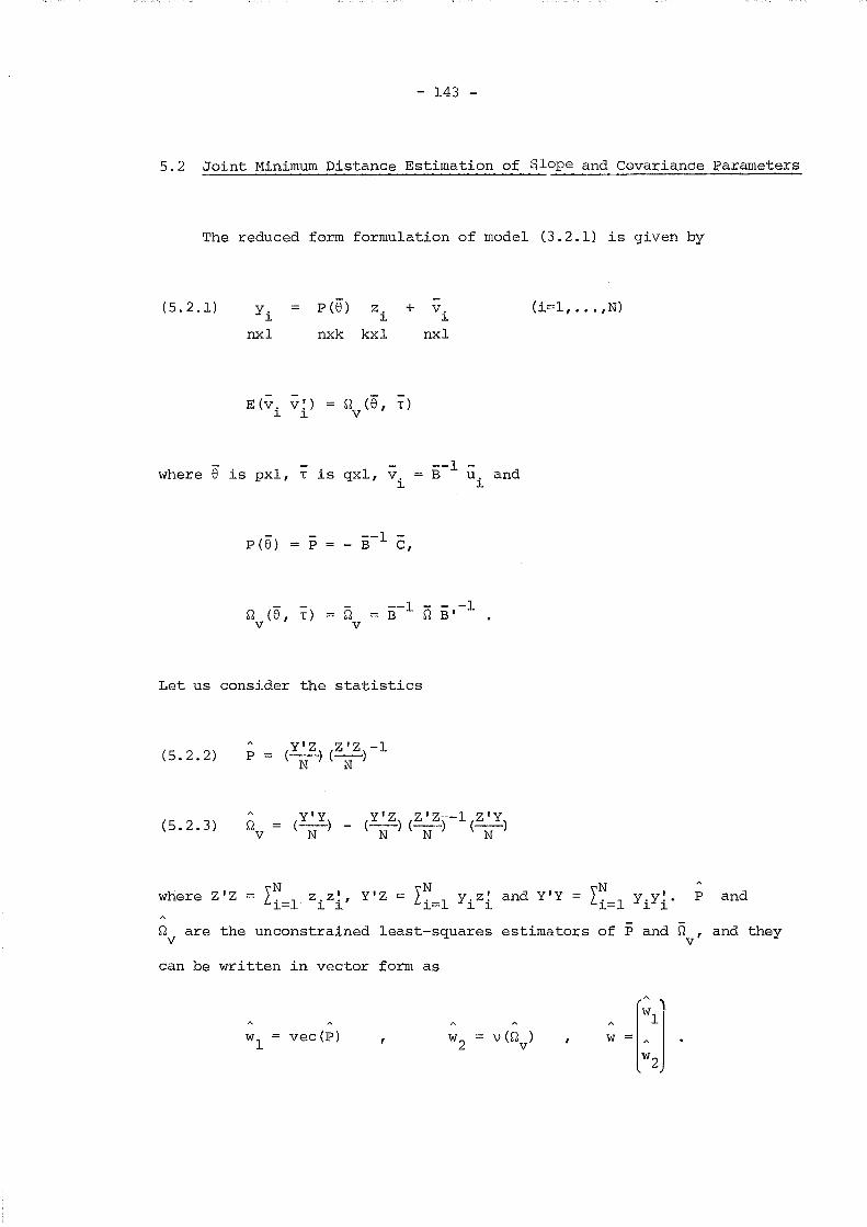
- 143 -

5.2 Joint Minimum Distance Estimation of Slope and CQvaria.nce )?arameters

The reduced form formulation of model (3.2.1) is given by

(5.2.1) P (6) z.~

nxk kxl

+ v.~

nxl

(i=l, ... ,N)

E(v. v ~ ) r2 (6, T)~ ~ v

6 --1 -where is pxl, T is qxl, v. B u. and~ ~

--1 -p(e) = p - B C,

fiv

Let us consider the statistics

(5.2.2)

(5.2.3)

p

r2v

(Y1Z) (ZIZ)-lN N

P andh I - IN "- IN 'd' - IN .,were Z Z - . 1 Z.Z., Y Z - . 1 y.z. an Y Y - . 1 y.y ..~=. ~ ~ ~= ~ ~ ~= ~ ~

r2 are the unconstrained least-squares estimators of P and fi , and theyv v

can be written in vector form as

vec(P) vW )v

w

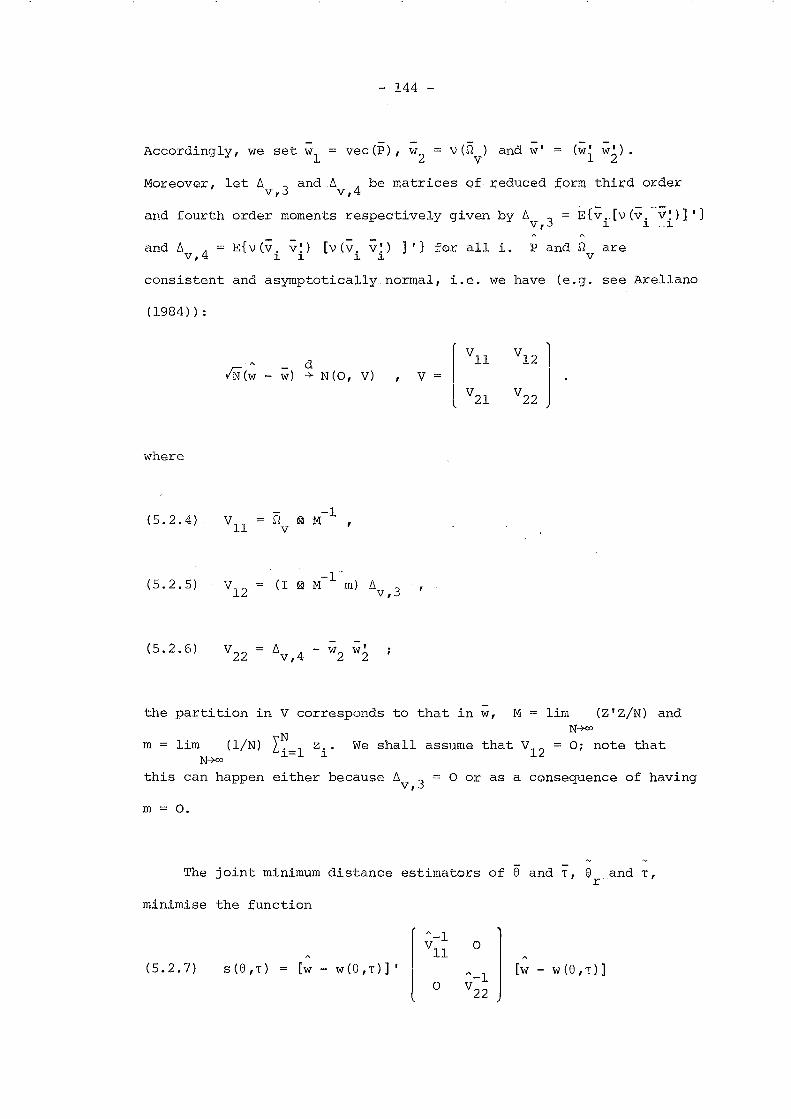
Accordingly, we set wl

- 144 -

vCS1 ) and w'V

(.w-, w-')1 2 .

Moreover, let 6 3 and 6 be matrices o~ xeduced torm third orderv, v,4

and fourth order moments respectively given by 6v,3

and 6v,4 E{VC~. ~~) [vC~' ~~) ] ,} for all i. P and n arel l l l V

consistent and asymptotically normal, i.e. we have (e.g. see Arellano

(1984)) :

where

.(5.2.4)

(5.2.5)

dw) -+ NCO, V)

n e M-I ,v

(1 e M-1 m) 6v,3

v

If Vu

V21

(5.2.6) 6v,4

the partition in V corresponds to that in w,

6 = 0 or as a consequence of havingv,3

m = lim (l/N) L~ 1 Z.. We shall assumeN-+oo l= l

this can happen either because

M = lim (Z'Z/N) andN-+oo

that V12

= 0; note that

m = o.

The joint minimum distance estimators of e and T, e and T,r

minimise the ~unction

o

(5.2.7) S(e,T) [w - Wce,T)]'

o[w - W(e,T)]

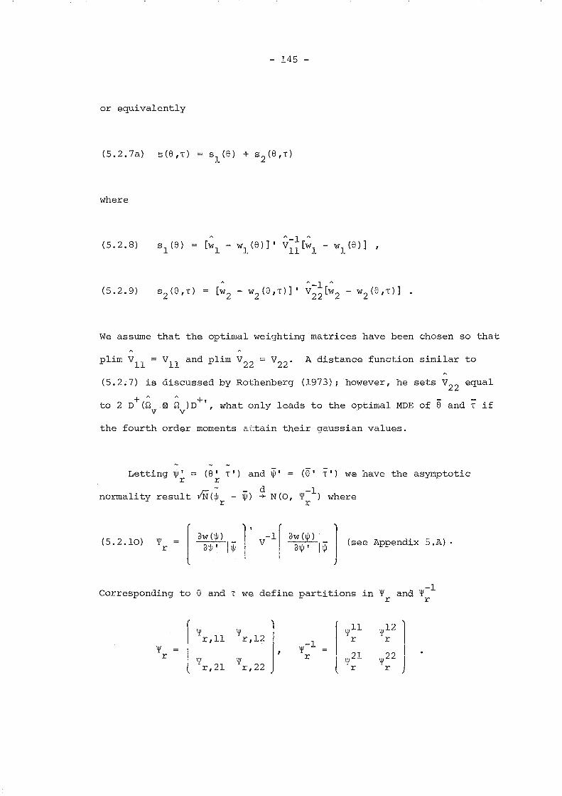
- 145 -

or equivalently

(5.2.7a) S(6,T)

where

(5.2.8)

(5.2.9)

We assume that the optimal weighting matrices have been chosen so that

plim Vll

= Vll and plim V22 = V22 . A distance function similar to

(5.2.7) is discussed by Rothenberg (1973); however, he sets V22

equal

to 2 D+(Q ~ Q )D+', what only leads to the optimal MDE of e and T ifv v

the fourth order moments attain their gaussian values.

Letting 1/J'r

(6' T') and ~,r

(8' T') we have the asymptotic

result ffl(1/J - ~)d If!-l)normality -+ N(O, wherer r

(5.2.10) If! [CJw (1/J) l' v-lf CJw(1/J)

1(see Appendix 5.A) .r CJ1/J ' I~ I CJ1/J ' I~

J

Corresponding to 6 and T we define partitions in If'r

-1and If'

r

If'r,2l

If'r

(

I If'r,ll

lIf'r,12

If' r,22

-1If'

r 1f'22r

- 146 -

In this context, we shall say that particular estimators o~ e and T

- 11 22are efficient if they attain the same AVM as e and T, ~ and ~

r r r

respectively. We have assumed ~ 4 to be finite and unrestricted;v,

alternatively we could consider a set of constraints in ~4 (e.g. in the

random effects model this can be done by assuming independence between

error components and that the fourth order moments are homoscedastic

over time) in which case more efficient estimators could be obtained

by including a further set of statistics in the definition of (5.2.7).

Thus, the estimators we propose, represent a feasible compromise: if

constraints are enforced in fourth order moments, determining their

sampling variances would require the evaluation of eighth order moments.

The same reasoning could apply to the latter and the process would

have no end.

If the errors are normally distributed ~ equalsr

<Pr plimN-+co[- (1/N)i>'d2

Lr /<l1V'd\)J I I~] where Lr is the log-likelihood

function associated to our model. But in general, \)Jr will be efficient

relative to the QML estimator since the latter is asymptotically

equivalent to the MDE whose norm converges in probability to

[n~; ® M 0 -ID I (~-l

I~ ® ~-l)D I

vv -'

which is not optimal.

The relation between the reduced form and the structural form

covariance matrices can be written in vector form as

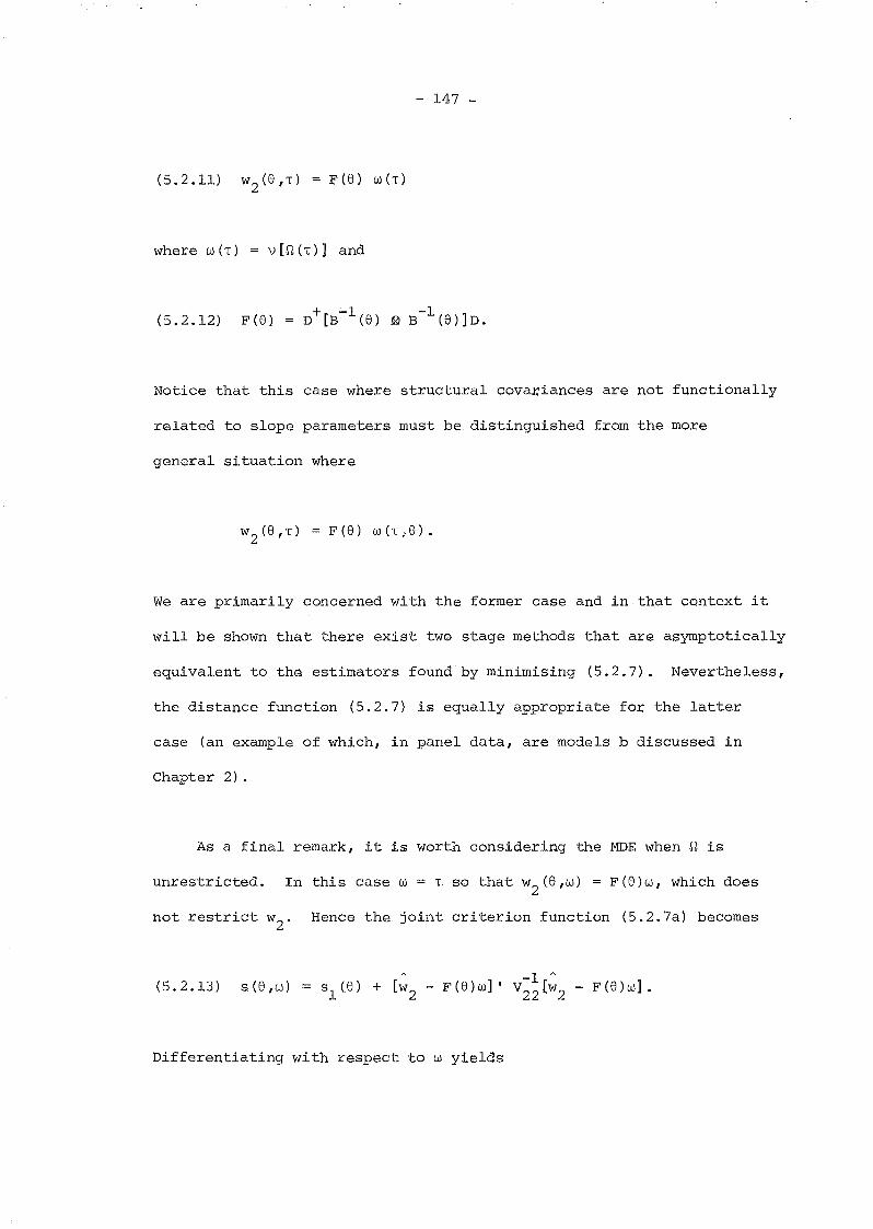
- 147 -

)'i'(8) wC-r)

where WeT) V[Q(T)] and

(5.2.12) F(8)

Notice that this case where structural covariances are not functionally

related to slope parameters must be distinguished from the more

general situation where

F (8) W (T ; 8) •

We are primarily concerned with the former case and in that context it

will be shown that there exist two stage methods that are asymptotically

equivalent to the estimators found by minimising (5.2.7). Nevertheless,

the distance function (5.2.7) is equally appropriate for the latter

case (an example of which, in panel data, are models b discussed in

Chapter 2).

As a final remark, it is worth considering the MDE when Q is

unrestricted. In this case W = T so that w2

(8,w) = )'i'(8)w, which does

not restrict w2

. Hence the joint criterion function (5.2.7a) becomes

(5.2.13) s(8,w)

Differentiating with respect to w yields

ds(8,w)dW

- 148 -

A_l A- 2 F I (8) V

22[W

2- F(8)w] = 0

A_lbut since F I (8) V

22is an ~ n(n+l) x ~ n(n+l) nonsingular matrix,

the MDE of w is just

or equivalently

(5.2.15) ft B (8) ft B I (8) •v

SUbstitution of (5.2.14) in (5.2.13) immediately reveals that the

concentrated distance function is simply sl (8). The minimiser of

sl(8), 8u

say, is the standard Malinvaudls minimum distance estimator of

a simultaneous equations model without covariance constraints, which

is well known to be asymptotically equivalent to the 3SLS and

ft-unrestricted QML estimators of e, 83SLS

and 8u

• Alternatively,

the IQML-type l of estimator of ft unconstrained takes the form

(5.2.16) ft A(8) (XIX) AI (8).N

Both ft and ft can be regarded as functions of 8 which provide a range

of asymptotically equivalent estimators of Q when evaluated indistinctly

at 8u ' 8u or 83SLS • The AVM of these estimators is given by Wu ,22 in

(3.4.3) .

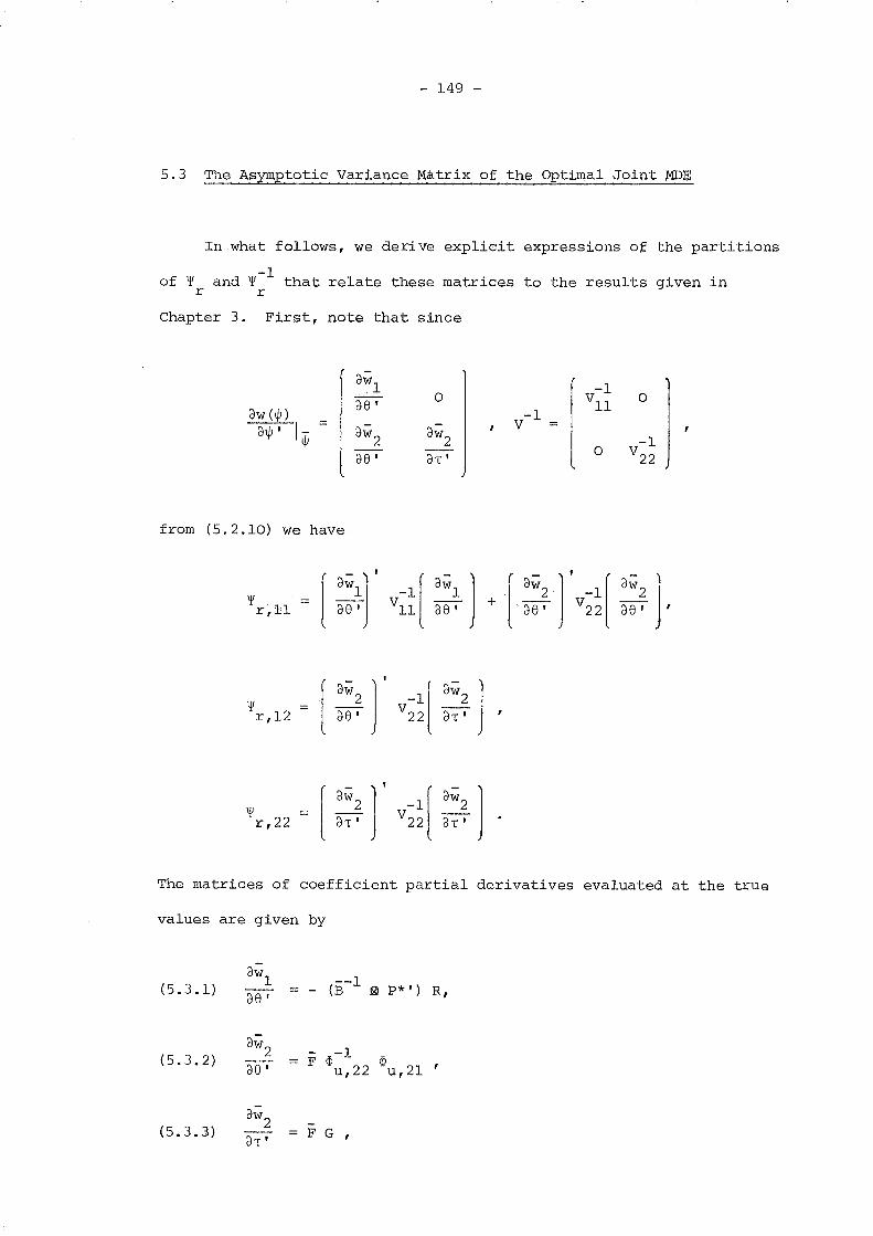
- 149 -

5.3 The As~totic Variance Matrix of the Optimal Joint MDE

In what follows, we derive explicit expressions of the partitions

-1of ~ and ~ that relate these matrices to the results given in

r r

Chapter 3. First, note that since

r oWl0

-10

dW (l/J) Ide'

-1Vu

dl/J • 1- dW2

dW2

VljJ I -1

l de • dT •0 V

22

from (5.2.10) we have

[-)'

dWl~ -­r,ll - d8')

( - ]' [dw2 · -1[3Ei' V22

~r,12 [

dW2 ] ,

d8 '-1[(V22

~r,22 [

dW2 ] ,

dT'

The matrices of coefficient partial derivatives evaluated at the true

values are given by

(5.3.1)dWl

(B-1.@ p* I)- R,d8 I

(5.3.2)dW

2 - -1

d8 •F <P <P

u,21u,22

(5.3.3)dW

2= F G ,

dT'

- 150 -

where F F(e), <P-1

22 <p 21 i~ given in (3.3.4), an p*, Rand G areu, u,

defined in Section 3.2. 2 It is convenient to re-write V22 as a function

of the struotural form fourth order moments, thus we have

(5.3.4) I::.v,4 W W'2 2

Hence sUbstituting (5.2.4) and (5.3.1) to (5.3.4) in our previous

expressions, since all terms F cancel, we have

(5.3.5) '¥ (<Pll) -1 + <p-1 - - -1 -1

r,ll u,12 <pu, 22 (I::. 4-w w' ) <p <pu,21u u,22

(5.3.6) '¥ <p -1 - - -1r,12 u,12 <PU ,22 (1::. 4 - w w') G

- - -1'¥ = G' (1::.

4- w w') G

r,22

- - -1Note that under normality (1::.4

- w w') <Pu ,22' so that '¥r <P •r

Next, let us define the matrix '¥ such thatu

thus

'¥u,ll

'¥u,12

'¥u,22

'¥ r,ll

-1 - - -1<P u ,12 <P U ,22 (1::. 4 - w w') ,

- - -1(I::. - w w') ,

4

(5.3.8)

'¥u,ll

- 151 -

~u,'2G 1G''¥u,22G J

Using the formulae for partitioned inverses it is straightforward to

check that '¥ is the inverse of the matrix W in Section 3.4. Thenu u

(5.3.9)-1

'¥u

r Wu,ll

l Wu,2l Wu,22

Finally, in view of (5.3.8) and (5.3.9) we may apply the Lemma in

Section 3.3 to obtain

(5.3.1O) ,¥ll -1W 22 (I-P')

-1W - W W 22{I-P) W Wr u,ll u,12 u, w u, w u,22 u,2l

(5.3.11) ,¥22 (G'-1 -1

W G)r u,22

with G{G'-1 G)-l G' -1

P W Ww u,22 u,22

11 22 .'¥ and'¥ are the asymptotlc covariance matrices of e and T,

r r r

respectively. Remark that Wu,ll is the AVM of the Q-unrestricted QML

and MD estimator of e, eu and eu. Thus, since Wu

,22 is a positive

definite matrix, from (5.3.10) we always have

AVM{e ) < AVM{e )r u

irrespective of non-normality.

- 152 -

5.4 EfficientMDE of Covariance Parameters and Minimum Chi-square

Specification Tests of CovarianceConstraints

Chamberlain (1982) advocates the use of MD estimators to impose

restrictions on covariance matrices in the context of i.i.d. random

vectors with unrestricted mean. Chamberlain shows that in general

the ~LE of the constraint parameters is less efficient than the

optimal MDE. We show that these results hold true for structural

covariance matrices. Furthermore, separate (optimal) MDE of covariance

parameters based on efficient unrestricted estimators of Q are

efficient in the sense of attaining the same limiting distribution as

the joint estimators defined in Section 5.2.

Thus let us consider the following. criterion function

(5.4.1) S (T)A_l A

[w - W(T) ] I V [W - W(T) ]W

where W v cm and Q is indistinctly the 3SLS, the MD or the QML

estimator of ~ unrestricted. We assume that plimN+oo Vw-V is

W

positive definite. Let TMD be the minimiser of S(T), so that TMD

solves the following system of equations

(5.4.2) o .

In particular, if the restrictions in Q are linear and homogeneous,

i~e~ WeT) = G T where G is a matrix of known constants, an explicit

solution for T D is availableM

- 153 -

(5.4.3)

Note that since (5.4.3) is linear, rl('MD) may not be positive definite.A _ d

Recalling that !:N(w - w) + N(O, Wu

,22) and in particular, under normality,

Wu

,22 = ~~2, the asymptotic distribution of 'MD follows as an application

of the results in Appendix 5.A. Thus, we have that !:N(TMD-T) ~ N(O,W, (Vw))

where

(5.4.4) W (V ) = -(G' '.1-1 G)-l (G' V- l W '.1-1 G) (G' V- l G)-lT w w wu,22 w w

This result applies to general constraints and so G is the matrix

of partial derivatives dW(,)/ch' evaluated at the true values. (5.4.4)

makes clear that the optimal choice for V is k W 2' where k is anw u,2

-1 -1 \,,22arbitrary real number, in which case W, reduces to (G' W

u,22 G) x r '

further establishing that the optimal 'MD is fully efficient.

Now we can refer to our results in (3.3.10) and (3.4.6a). It

turns out that the QML estimator of , is asymptotically equivalent to

22the MDE that sets V equal to k ~ , and therefore it is generally

w u

inefficient relative to the optimal MDE. Only under gaussian kurtosis

(or in the special case where Wu

,22 is proportional to ~~2) QML and

optimal MD are asymptotically equivalent. Thus,

(5.4.5)

(5.4.6)

and

W (W 22) \j!22,u, r

W > \j!22 •r,22 - r

- 154 -

Minimum Chi-square Specification Tests of Covariance Constraints

The assumption that w depends on a q x 1 vector of parameters T

imposes r = ~ n(n+l) - q restrictions on w. Suppose that we wish to

test this set of constraints. In Chapter 4 we discussed Wald and

quasi-likelihood ratio tests; alternatively we can rely on the

statistic N°S(TMD), since we have the following result

(5.4.7) MCS N[w

Proof: See Chamberlain (1982, Appendix B, Proposition 8).

That is, under the null hypothesis N°S(TMD) is asymptotically

distributed as a X2 variate with r degrees of freedom if TMD is the

optimal MDE and an optimal norm is used in setting up the statistic,

i.e. plim Wu ,22 = Wu ,22.

The advantage of the statistic MCS is that it does not require

explicit expressions of the constraint equations. This feature

makes the minimum chi-square tests specially attractive in panel data,

where serial covariance matrices are initially expressed in terms of

constraint parameters. Moreover, notice that since separate MDE of

T based on Q are efficient, we do not require Q-restricted estimates

of the slope coefficients in setting up the minimum chi~square statistics.

Finally, suppose that we consider testing an additional set of

constraints T = T(K) where K is sXl(s~q). Then KMD

minimises

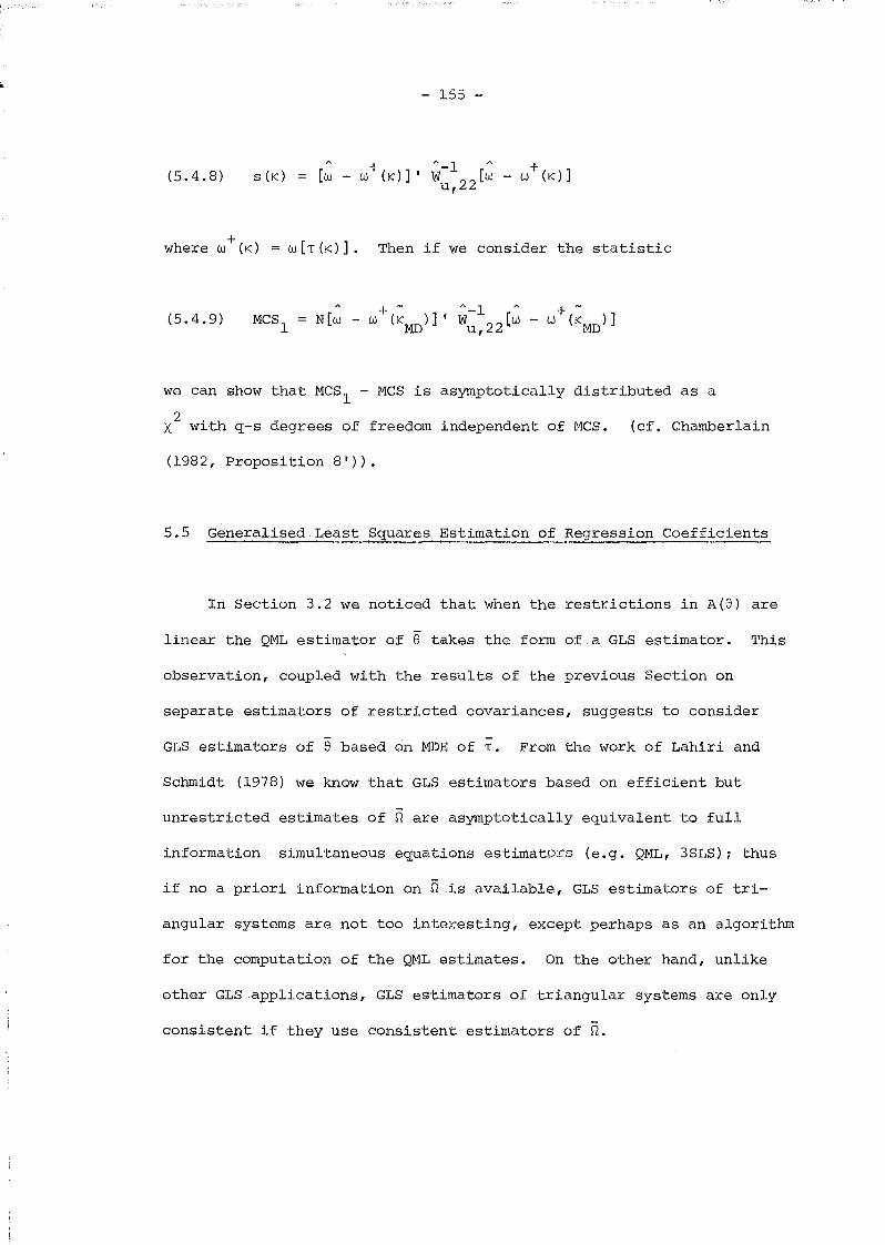
(5.4.8) S (K)

- 155 -

+where W (K) W[T(K)]. Then if we consider the statistic

(5.4.9) N[W

we can show that MCS l - MCS is asymptotically distributed as a

2X with q-s degrees of freedom independent of MCS.

(1982, Proposition 8')).

(cf. Chamberlain

5.5 Generalised Least Squares Estimation of Regression Coefficients

In Section 3.2 we noticed that when the restrictions in Ace) are

linear the QML estimator of e takes the form of a GLS estimator. This

observation, coupled with the results of the previous Section on

separate estimators of restricted covariances, suggests to consider

GLS estimators of e based on MDE of T. From the work of Lahiri and

Schmidt (1978) we know that GLS estimators based on efficient but

unrestricted estimates of n are asymptotically equivalent to full

information simultaneous equations estimators (e.g. QML, 3SLS)i thus

if no a priori information on nis available, GLS estimators of tri-

angUlar systems are not too interesting, except perhaps as an algorithm

for the computation of the QML estimates. On the other hand, unlike

other GLS applications, GLS estimators of triangular systems are only

consistent if they use consistent estimators of n.

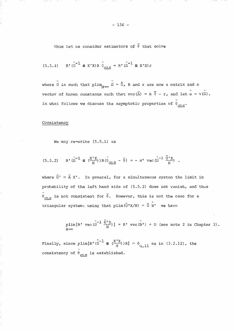
- 156 -

Thus let us consider estimators o£ 8 that solve

(5.5.1)~-l ~

R' (Q ~ X'X)R 8GLS

R' (~-l 2 X'X)r

where Q is such that pli~+oo Q Q, Rand r are now a matrix and a

vector of known constants such that vec CA) = R e - r, and let w = \! Cn) •

In what follows we discuss the asymptotic properties of 8 S.GL.

Consistency

We may re-write (5.5.1) as

(5.5.2)~-l U'X

- R' vecW --)N

where U' A X'. In general, for a simultaneous system the limit in

probability of the left hand side of (5.5.2) does not vanish, and thus

8GLS

is not consistent for 8. However, this is not the case for a

triangular system: using that plim(U'X/N) = S'i B' we have

~-l -,plim[R' vec(Q U X)]

NN+ooR' vec (B') o (see note 2 in Chapter 3).

--1 X'XFinally, since plim [R I W ~ CN )) R]

consistency of 8GLS

is established.

~ as in (3.2.12), theu,ll

- 157 -

Asymptotic Normality

If we regard C5.5.2) as a vector valued function of w, using a

first order expansion about wand resca1ing we can write

(5.5.3) [R' C;'-l ® X~X)RJ IN"C$GLS - 8) '"

where w* = vC~*) lies between wand w. Now notice that since

plim ~* = fi, in view of (3.2.13) we have plim[R' (I ~ X'u) (~-1 ~ ~:l)D] = - ~N * u,12

so that

(5.5.4) ~ 11 IN (8 GLSu,w) + 0 (1).

p

Next, assuming that ~ ~(TMD) where 'MD minimises a distance

function of the type (5.4.1), if we define the indempotent matrix

P= = G(G' v-1 G)-l G' v-1 , we havev w w

(5.5.5)A

p- !N(wv

w) + 0 (1).p

Thus, (5.5.4) becomes

(5.5.6) ~ 11 !NC8 GLSu,1 --1 -- R' vec W U'X)!N

~ F- !N(~u,12 v

w) + Q (1)p

3Moreover, it can be proved that

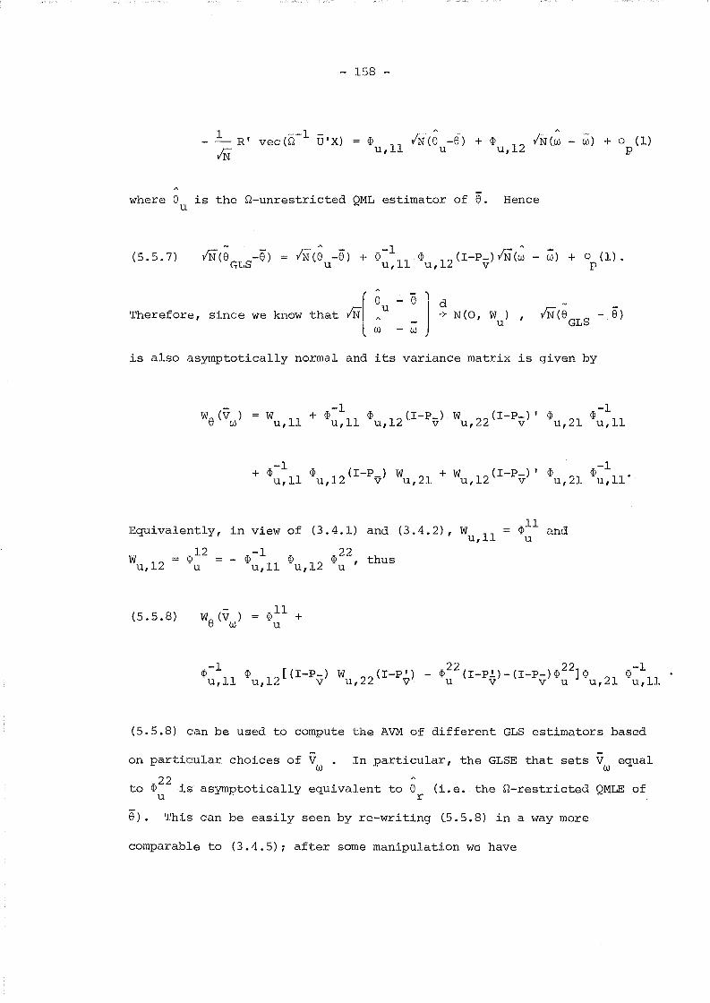
- ],'38 -

:=: IN (.e -8) IN(.~~u,ll u + ~u,12 w) + 0 (1)p

where 8 is the ~-unrestricted QML estimator of 8. Henceu

(5.5.7) !Nee -8) + ~-l ~ 12(I-l?-)!N(~ - w) + 9 (1).u u,ll u, v P

Therefore, since we know that- e

- w] ~ N(O, W )

u m(e SGLe)

is also asymptotically normal and its variance matrix is given by

-1 -1Wu,ll + ~u,ll ~u,12eI-l?v) wu ,22 (I-P:;:;) , ~u,21 ~u,ll

Equivalently, in view of (3.4.1) and (3.4.2), Wu,ll

~ll andu

Wu,12

(5.5.8)

~12u

ffi- l ffi ffi22 h'J! 'J! 'J! t usu,ll u,12 u'

~ll +u

~-ll1 ~ l2[(I-P-) W 22(I-P') - ~22(I_P~)_(I_P_)~22]~ 21 ~-1u, u, v u, V u v v u u, u,ll

(5.5.8) can be used to compute the AVM of different GLS estimators based

-on particular choices of Vw

In particular, the GLSE that sets V equalw

ffi22. . 1 . 1 e (. () dto 'J! ~s asymptot~cal y equ~va ent to .~.e. the ",-restricte QMLE ofu r

8). This can be easily seen by re-writing (5.5.8) in a way more

comparable to (3.4.5) ; after some manipulation we have

- 159 -

iP-1

iP 12{ (!-P.,.) [iP22

_ (6.4

-6.411

)] Cl:-Pvl.)u,ll u, V u

+ p_ iP 22 (I_Pl.) + (l-P-) iP 22Pl.}

V u V V U V

Simply noting that P~ iP22

(1_Pl.) = 0 it follows that'J! u V

(5.5.9) Wr,ll

-Another intuitively relevant choice for Vw is Wu ,22' that is,

the GLSE of e that uses the optimal MDE of T. Under normality

We (Wu ,22) = We(iP~2), but in general the matrix We(iP~2) - We (Wu ,22) is

indefinite. Making use of (5.5.-8) after some reductions we have

+ (p -P~) (W 22-iP22 ) + (W 22-iP22 ) (P'-P;)]<P 21 iP-lllw 'J! u, U u, u W 'J! u, U,

and although (Pw-PiP ) Wu,22(P~-P~) is positive semi-definite, the

matrix in square brackets on the right hand side of (5.5.10) is

indefinite. Therefore, none of these two estimators is generally

efficient in the sense introduced in Section 5.2.

An Efficient GLS Estimator

Let us consider the GLS estimator 8GLS

of the type (5.5.1) which

is based in the following choice of w:

(5.5.11) w = (1 ~22 W"-l) (~22 "_1 ) ( )- u u,22 w + u Wu ,22 w TOMD

Under normality, Wu,22

large relative to q,22u

- 160 -

1 , l' :22 ",22 d - 'h '1 Ewhere p 1m Wu ,22 = Wu ,22' p 1m ~u = ~u an TOMP 1S t e opt1ma MD

of T. Thus W is defined as a matrix-weighted average of wand W(TOMD

).

22 =-q, and then W = W(T ), but as W 22 becomes

u OMD u,

an increasing weight is being put on W relative

to W (TOMD

). We prove below that the GLS estimator so de:f;ined attains

the same AVM as the joint MDE 8 and is therefore efficient. Note thatr

since W is a linear combination of consistent estimators of w, it is

itself a consistent estimator of Wi though since W is an unrestricted

estimator of w, W will not satisfy the covariance restrictions.

To obtain the limiting distribution of 1N(8GLS

- 8), we begin

by re-writing (5.5.11) as

furthermore, using (5.5.5) with P in place of P- we havew v

Now applying (5.5.4) to the present case it turns out that

A

1N(8 -8)u

-1 A

W W 22 (I-P ) IN(w-w) + 0 (1)u,12 u, w P

where we have used the fact that Wu,12

q,-l q, q,22u,ll u,12 u

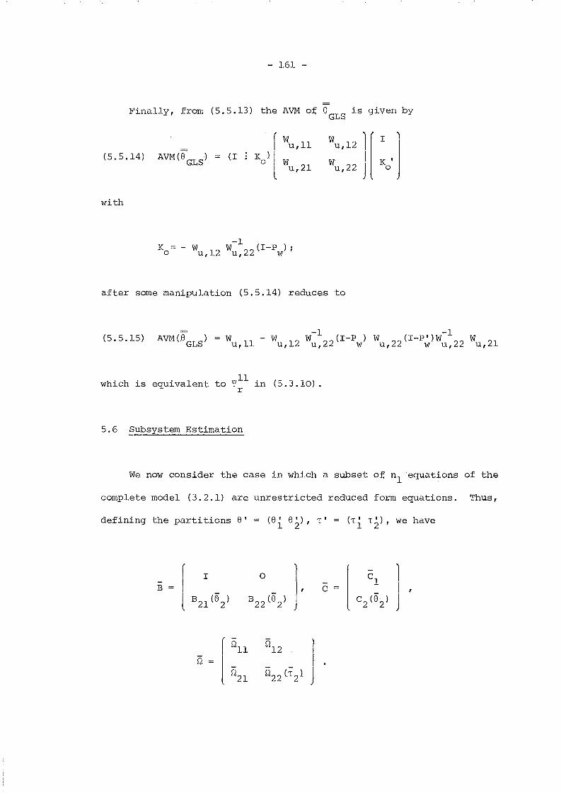
- 161 -

Finally, from (5.5.13) the AVM of 6GLS

is given by

( W Wu ,12 1[" lI u,ll

(5.5.14) AVM(8GLS

) (1Ko) lw W I K' Ju,2l u,22 J 0

with

-1K = - W 12 W 22 (I-P ) io u, u, w

after some manipulation (5.5.14) reduces to

(5.5.15) AVM(BGLS

) Wu,ll

which is equivalent to ~ll in (5.3.10).r

5.6 Subsystem Estimation

We now consider the case in which a subset of n l equations of the

complete model (3.2.1) are unrestricted reduced form equations. Thus,

defining the partitions 8' = (8i 82), T' = (Ti T2), we have

r1 - 11 0 Cl- j. - IB C

l B21

(62

) B22

(82

) C2

(82

)J

r- Q

12)

s-lU

Is-l l s-l2l Q22 eT2), J

- 162 -

-~ll' ~12 and Cl are unrestricted matrices whose coe~~icients c~n be

arranged in the vectors T1 and 81

, and B22 (82

) is lower tri~nguler.

(3.2.1) then becomes

(5.6.1)-

Yli + Cl zi

nlxk

- -(5.6.2) B21 Y

li+ B22 Y2i + C

2zi

n2

xnl

n2

x n2

n 2xk

A2 (82 ) xi u2in

2xl

the restrictions in A2

are linear so that

R 0Jl, r ~ f

l

rr1

2

J1

, vec(A2

1R2

R2

82

- r2

in particular note that Rl

= Kl~) where Kis the commutation matrix

2of order n 1 (nl+k), ° is a n

lx nlk matrix of zeroes and I is a nlk unit

matrix. Also let us introduce a notation for the partition of ~-l

-1~ [:::

Clearly the estimator that solves

(5.6.3)--1

X'X)R2

82

--1X'x)r

2R;W22 ~ R;W22~

(with plim ~22 ~22) is inconsistent for 82 unless ~12 0.

4

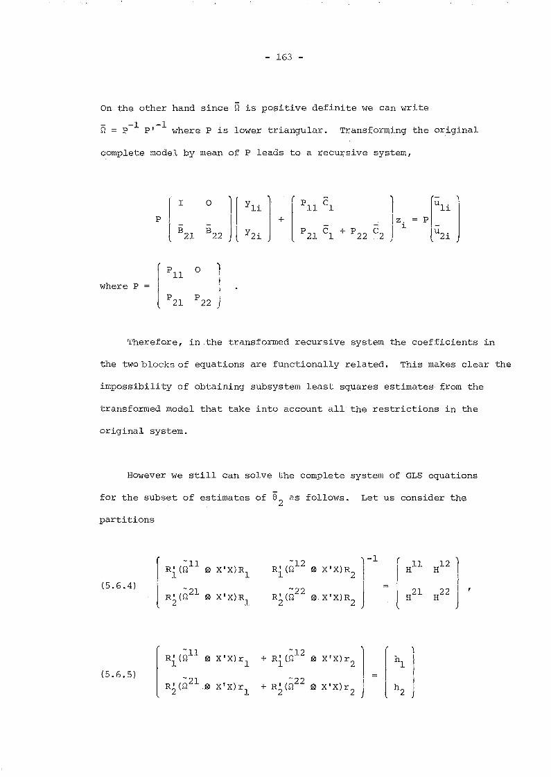
- 163 -

On the other hand since fl is positive definite we can write

- -1 -1~ = p pI where P is lower triangular. Transforming the original

complete model by mean of p leads to a recursive system,

rI 0

11 Yli(

Pll Cl 1 p[llli 1IP

+ l Iz.

l- -

Jl- J l lU2i

B21

B22 Y2i P21 Cl + P22C2

[Pll 0

]where PP

21 P22

Therefore, in the transformed recursive system the coefficients in

the two blocks of equations are functionally related. This makes clear the

impossibility of obtaining subsystem least squares estimates from the

transformed model that take into account all the restrictions in the

original system.

However we still can solve the complete system of GLS equations

for the subset of estimates of 82

as follows. Let us consider the

partitions

r R' (Qll R' (Q12 1-1 (Hll

H12

0 X'X)Rl

0 X' X)R2 l1 1

(5.6.4) lR' (Q21 R' (~22J

21 22@ X'X)R

l 0 X'X)R2 H H

2 2

R' (Qll + Ri (;12

] r

'\0 X'x)r

l0 X'x)r

2 hl1(5.6.5)

R' (Q21 + R;(Q22 ~o X'x)rl

X'x)r2 l h 22

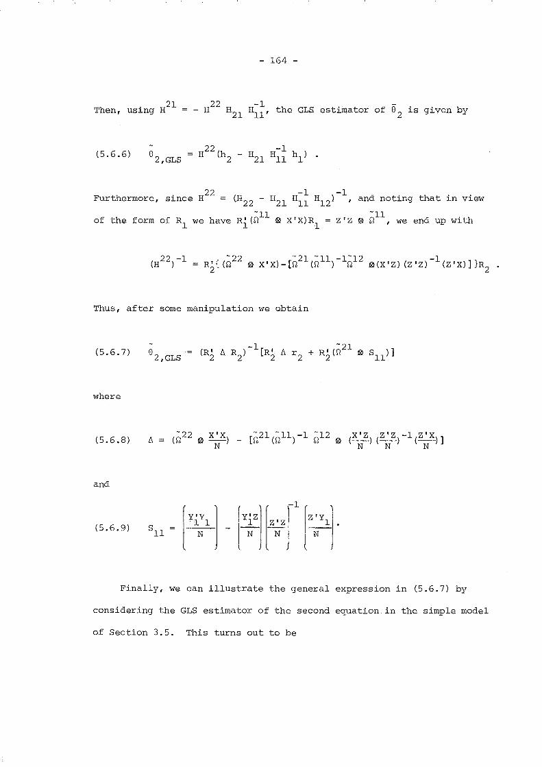
Then, using H2l

- 164 -

- H22

H2l H~~, the GLS estimator of; 82 is given by

(5.6.6) H22 (.h2 -1 h )- H2l Hll 1 .

22 -1-1Furthermore, since H = (H22 - H2l H

llH

12) , and noting that in view

of the form of; Rl

we have R' (;11 ~ X'X)R = z'z ® ;11, we end up with1 1

Thus, after some manipulation we obtain

(5.6.7)

where

(5.6.8)

and

(5.6.9)

Finally, we can illustrate the general expression in (5.6.7) by

considering the GLS estimator of the second equation in the simple model

of Section 3.5. This turns out to be

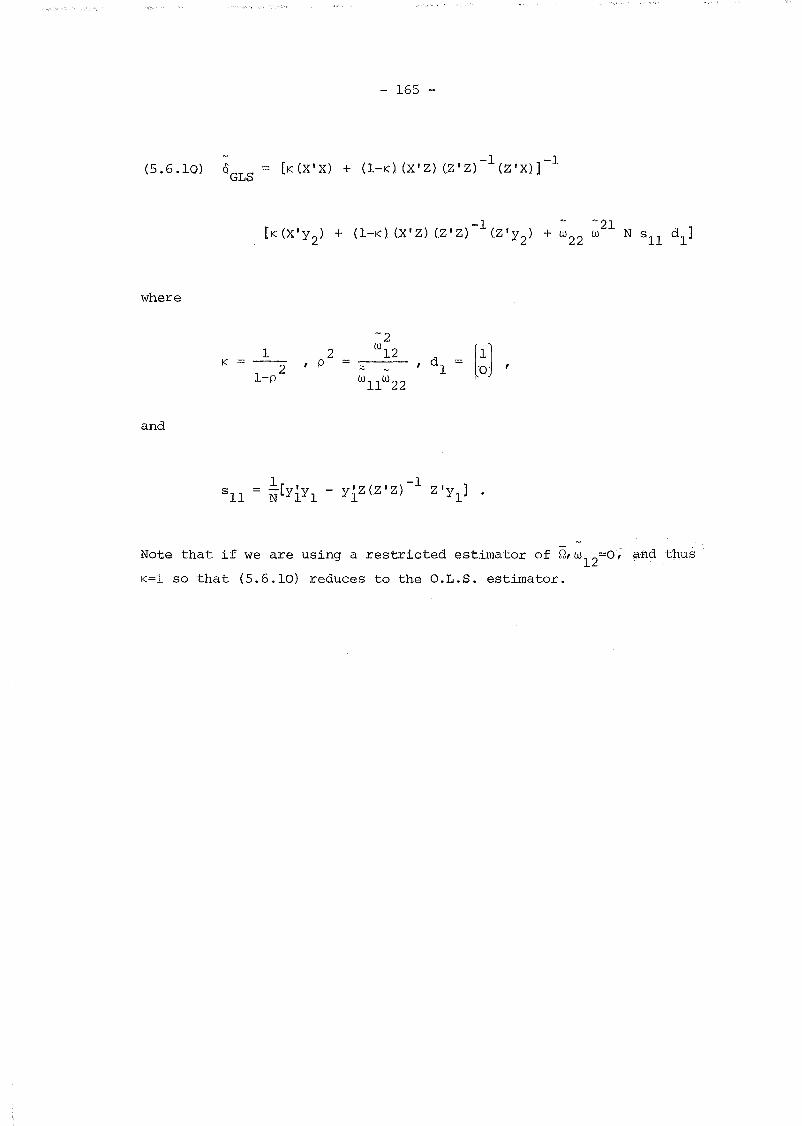
- 165 -

(5.6.10) 0GLS

where

and

K = 121-p

2p l~J '

Note that if we are using a restricted estimator of Q'W12=0;~nd thus

K=l so that (5.6.10) reduces to the O.L.S. estimator.

- 166 -

NOTES

1 The results given in Sections 5.4 and 5.5 are a revised ve~sion

of those given in Arellano (1985).

2 In the derivation of (5.3.1), (5.3.2) and (5.3.3) we have made

use of the result d vec(A- l ) = - (A ~ A,)-l d vec(A) , t'or non-

singular A. The matrices of partial derivatives are immediately

determined from the differential by noting that for an n x 1 vector

valued function t of an m x 1 vector 8 we have

dt.(8)J

m

Lk=l

(j=l, .•• ,n)

or equivalently d t(8)dt (8)

d8' d 8.

3 Using X Z p*' + UB' and (3.2.13) We have

--1 -R' vecW U'X) R' vec(Q-l u'ZP*')

moreover since <I> w = 0 for a triangular model (see note 2,u,12

Chapter 3), this is equivalent to

1 --1--R'vecW U'X)IN

Now using

1 --1-- R'vec(rG U'ZP*')IN

<I> IN[N1 v (U'U) - w] .

u,12

- 167 -

11 1 --1-q> - R'vecW U'Zl?*') + q (1)

u IN J?

and noting that Cl. first order eXJ?ansion of IN(~-w) about 8 yields

IN1~ V (D'D)N

q> -1 q> /N(e -8) + 0 (1)u,22 u,21 u P

Wla have

1 --1-- _. R'vec(Q U'X)IN

from which the result claimed follows.

4 (5.6.3) can be re-written as

Then noting that plim (D' X/N)2

Plim(D;D B'/N) we have that

I)B' ]

After some reductions it turns out that a typical element of this

vector takes the form

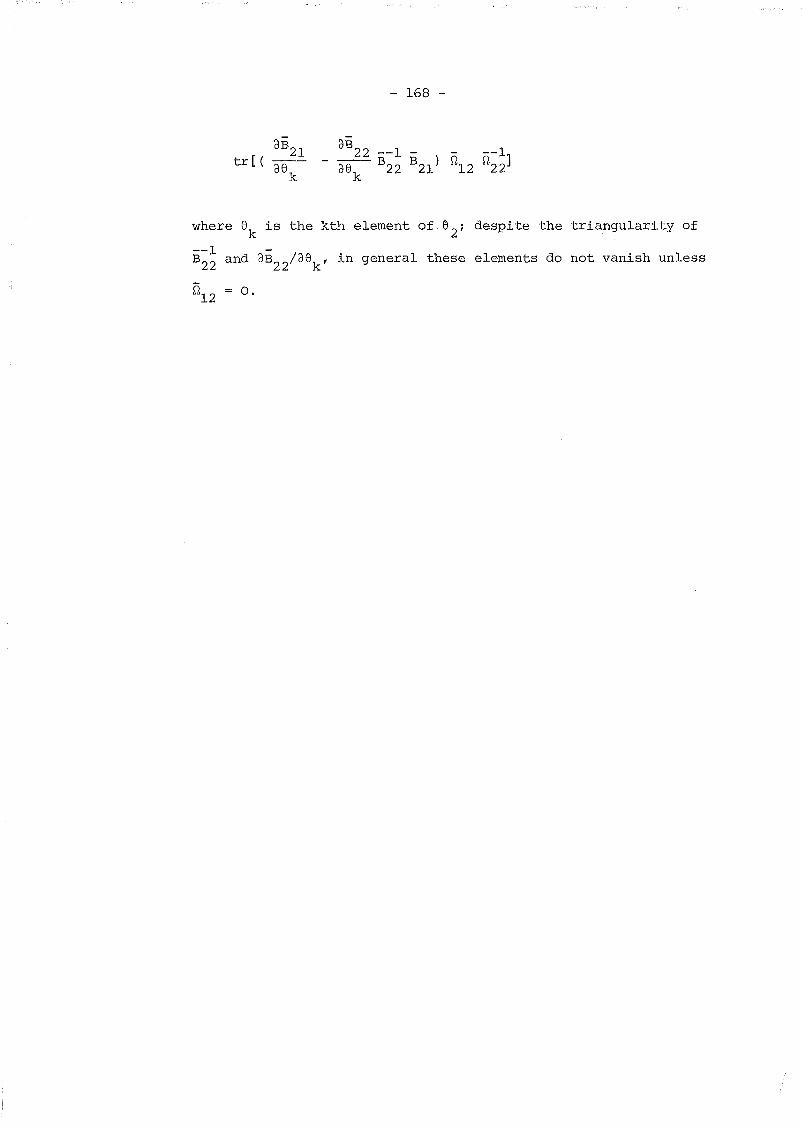
- 168 -

where Sk is the kth element of S2; despite the triangularity of

--1 -B

22and 3B

22/3S

k, in general these elements do not vanish unless

S1l2 = o.

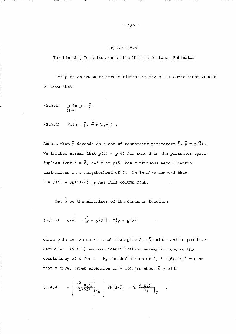
- 169 -

APPENDIX 5.A

The Limiting Distribution of the Minimum Distance Estimator,

Let p be an unconstrained estimator of the s x 1 coefficient vector

p, such that

(5.A.l) plim p p ,N-7<X>

A d(5.A.2) vN(p - p) -+ N(O,V ) .

P

Assume that p depends on a set of constraint parameters 6, p p (8) •

We further assume that p(o) = p(8) for some 0 in the parameter space

implies that 0 8, and that p(o) has continuous second partial

derivatives in a neighborhood of 8. It is also assumed that

D= D(8) = op(o)/oo' 18

has full column rank.

Let 0 be the minimiser of the distance function

(5 .A. 3) s (0) [p - p (0 ) ]' Q [p - p (0 ) ]

where Q is an sxs matrix such that plim Q Q exists and is positive

definite. (5.A.l) and our identification assumption ensure the

- -consistency of 0 for 6. By the definition of; 0, 0 8(0)/0010 = 0 so

that a first order expansion of d sun /os about 8 yields

(5.A.4) _ [ 02

s (0 )1 ]. cN (; _1")0000' 0* VN u u

vN 0 s (<$)

00 1 8

.. - 170 -

where 0* lies between 0 and 6. NOW since

(5.A.5)d s(o)

dO 18- 2 6' Q[p - p(8)]

in view of (5.A.2) we have

(5.A.6)Cl s (0)

dO l­e

d-7- N(O, 4 D'Q v Q6).

p

On the other hand, since plim 0* 6, direct evaluation shows that

(5 .A. 7) plimN-+<x>

2 01 Q D

Hence, using the Cramer linear transformation theorem

(5.A.8)

where

(5.A.9)

-1Clearly, an optimal choice for Q is V , in which case the asymptotic

p

covariance matrix of Q reduces to

(5.A.IO) Vo-1 - -1(6 I VD) •P

- 171 -

CHAPTER 6

EFFICIENT MD AND GLS ESTIMATORS APPLIED TO PANEL DATA

6.1 Introduction

The methods developed in Chapter 5 suggest an estimation and

modelling strategy for dynamic models from panel data. Regression

specification analyses can be based on ~~unrestricted 3SLS or QML

estimates of alternative versions of the model under consideration

(though 3SLS estimates have the advantage of not requiring iterative

optimisation). Once a particular specification has been chosen we

can proceed to estimate and test different structures for ~ using

minimum distance estimators and minimum chi-square or Wald tests.

If eventually a particular covariance specification is not rejected,

this information can be used to obtain more efficient estimates of the

regression parameters by mean of the GLS procedure discussed in

Sections 5.5 and 5.6. A computer program has been written in Fortran 77

to perform the calculations involved in this sequence.

This Chapter discusses the application of the results in Chapter 5

to panel data, and also various calculations are performed to assess

the practical performance of the proposed methods. Section 6.2 presents

the analytical results and in Section 6.3 a simulation is carried out

and the Michigan earnings function is re-estimated.

- 172 -

6.2 The Estimators

We begin by considering in some detail the MD estimation of first

order moving average covariance structures. W~ use the same notation

as in Chapters 2 and 4. The T x T random effects MA(l) covariance

matrix may alternatively be parameterised as

(6.2.1)

where

222o (HA ) + 0 n

2on

2 2A, 0 and On can be easily retrieved from gl' g2 and 93 by noting that

2A solves A - c A + 1 = 0, with c = (gl-g3)/(g2-g3)' so that

(6.2.2)

(6.2.3)2

o

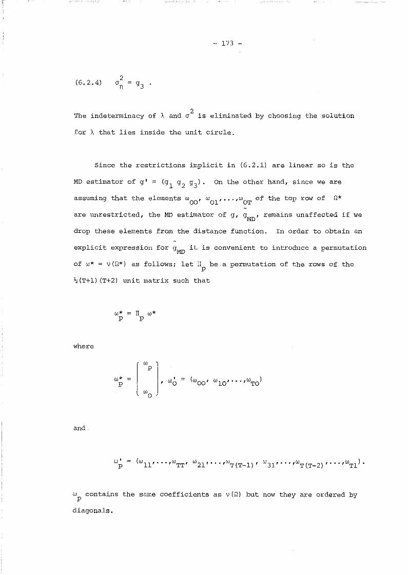
(6.2.4)2

(Jn

- 173 -

2The indeterminacy of A and (J is eliminated by choosing the solution

for A that lies inside the unit circle.

Since the restrictions implicit in (6.2.1) are linear so is the

MD estimator of g' = (gl g2 g3)· On the other hand, since we are

assuming that the elements woo' wOl, •.. ,wOT of the top row of Q*

are unrestricted, the MD estimator of g, gMD' remains unaffected if we

drop these elements from the distance function. In order to obtain an

explicit expression for gMD it is convenient to introduce a permutation

of w* = v(Q*) as follows; let IT be a permutation of the rows of thep

~(T+l) (T+2) unit matrix such that

W* IT w*p p

where

rW "\p

J·w* ,

(woo' WlO,··· ,wTO )p

lWo

Wo

and

W'P

W contains the same coefficients as v(Q) but now they are ordered byp

diagonals.

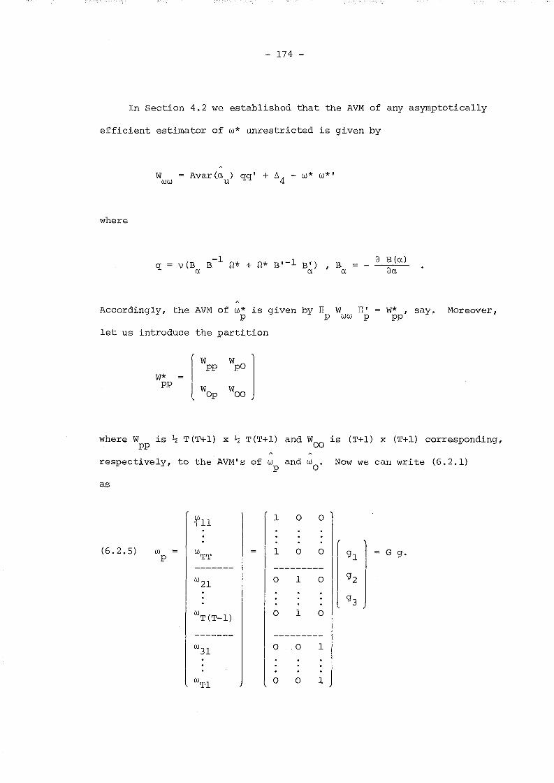
- 174 -

In Section 4.2 we established that the AVM of any asymptotically

efficient estimator of w* unrestricted is given by

where

q \J(B B-1 st* + st* B,-l B I )

a aB

ad B Ca)

da

Accordingly, the AVM of w* is given by IT W IT' W* , say~ Moreover,p p ww p pp

let us introduce the partition

rW W

po IppW* jpp

l Wop WOO

where W is ~ T(T+l) x ~ T(T+l) and WOO is CT+l) x (T+l) corresponding,pp

respectively, to the AVM's of wp

and wO. Now we can write (6.2.1)

as

- 175 -

tUg'''i minimises

MD

s (g)

thus obtaining

".-1 "(w - G g)' W (1J) - G g)

P pp P

(6.2.6)"-1 1(G' W G)- Gpp

"-1 "W w

pp p

where W is a consistent estimator of Wand w is an asymptoticallyW W p

efficient estimator of w unrestricted. Incidentally, note that ifp

we replace ~-l by an unit matrix we obtain a 'crude minimum distance'pp

estimator; this estimator is consistent although inefficient, and in

view of the form of the matrix G, crude MD estimators of gl' g2 and g3

are simple arithmetic means given by

T1 \'

(T 1) L wt (t-l)- t=2

1T*

where T* = ~ T(T+l) - T - (T-l). We further remark that (6.2.6) does not

impose the restrictions g3 > 0 and (gl-g3) > 0 and thus it is not

2 2guaranteed that the implied estimates for cr and 0 will be positive.

n-2 -2

However, significantly negative values of 0 and/or 0 will commonlyn

be an indication of misspecification. A minimum chi-square test of the

structure (6.2.1) is given by

(6.2.7) MCS

- 176 -

A_l AN (W - G gMD) , W (W

p pp p

2MCS is distributed as a X with ~ T(T+l)-3 degrees of freedom under

the null hypothesis.

Once gMD has been obtained, we may proceed to calculate the MD

estimator of wo' wo. This is only necessary if the slope parameters

are going to be re-estimated by GLSi Wo is given by

(6.2.8)

where Wop

is a consistent estimator of Wop

and Wo is an asymptotically

efficient Q*-unrestricted estimator of wO.

The previous results can be generalised to higher order moving

average schemes. If we consider an sth order moving average case (with

s < T - 1), Q will depend on s + 2 constraint parameters

2A

2 A2) 2gl (J (1 + + ... + + (J

1 s n

2+ A1A2 +... + As_1A s )

2g2 o (A

l+ (J

n(6.2.9)

2A

2gs+l

(J + 0S n

2gs+2

(J

n

where vit = €it + Al €i(t-l)+···+ As €i(t-s)· Again, Al,··.,A s ' 02

and (J~

can be retrieved from gl, ..• ,gs+2 by solving the nonlinear system (6.2.9).

- 177 -

However, note that if the only purpose in enforcing the restrictions

in ~ is to obtain GLS estimates of the slope parameters, there is no

need to retrieve the moving average coefficients.

Finally, if autoregressive or ARMA schemes have to be estimated,

the corresponding distance function will have to be minimised by

mean of iuerative techniques.

GLS Estimation of a, Sand y

This is a particular case of the problem of subsystem estimation

studied in Section 5.6; there is only one unrestricted reduced form

equation and it corresponds to the prediction equation for Yo. Let

(6.2.10) \! W*) (I - WA-l)~* +:;:; wA. -1 * ( . )

...... 'ww . ww -'ww ww w gMD' Wo

Where M is a consistent estimate ofww

as given in (4.2.9).- ww

~* is the estimate of ~* that leads to the optimal GLS of 8' = (a S'y')

robust to non-normality (NNGLS). Moreover, let us introduce the

partition

=00 =01w w~*-l

10 11w ~

=11 =t.s =01 =01 =OTand let ~ = {w } and w = (w , •.. ,w ). Then, direct application

of the results in (5.6.7), (5.6.8) and (5.6.9) gives

(6 . 2 . 11) 8GLS+' + -1 +'

(X IJf X) (X IJf y + 1jJ d1

)

- 178 -

where

11 -1 10 =01 =00(IN .® ~ ) - [z* (z* , z*) 'Z*'.® w w /w ],

T

Lt=l

~t , (I.Yt-l·

-1z* (z* , z*) Z* ') Y

o

and dl

is an (n+m+l) vector with one in the first position and zero

elsewhere. Finally, in view of the discussion in Section 2.4, a

computationally more convenient expression for 0GLS is given by

(6.2.12) °GLS rT T

_I I (~s X+t ' X+

t=l s=l s

=to=so A+'W w=00 Xtw

[

T

Lt=l

T =to=so\ =ts +' W W +'L (w X

tY - X

s=l s ~o tY) + 1jJ

s

6.3 Numerical Results

Two Monte Carlo experiments were conducted in order to investigate

the performance of GLS and MD estimators, particularly the magnitude

of the finite sample efficiency increase that results from covariance

restrictions. The performance of minimum chi-square tests was also

examined. The present experiments were based on the same model we used

in Section 4.4. However, a shorter number of replications (30 samples)

were generated in this case due to CPU time limitations. Tables 1, 2

and 3 summarise the results. For the normal model, the biases in the

3SLS estimates are of a similar magnitude to the biases in the QML

- 179 -

estimates corresponding to the moving average data reported in Chapter

2; however, the finite sample variances appear to be smaller in the

case of the 3SLS estimator. On the other hand, GLS estimators that

use the a priori information on the covariance matrix have in general

a smaller variance than the 3SLS estimator, although the reduction in

variance varies considerably from one parameter to another. For

example, considering the non-normal model, the variance of the NNGLS

estimate of a is cut by an amount of 22 percent of its 3SLS value, but

the variance reduction relative to NGLS is of only 2 percent. In the

case of the intercept, the NNGLS variance is 14 percent less than its

3SLS variance and 6.5 percent less than the NGLS variance, which is

also the case for Yl

. In the case of S there is no reduction at all.

Turning to MD estimates of covariance parameters (Table 2), in the

2 2nonnormal experiment the NNMD variances of 0 ,0 and A are reducedn

by an amount of 49.5, 1 and 24 percent of their NMD variances, respectively.

h b ' h 2 d 2 ,However, t e lases in t e NNMD estimates of 0 an 0 are respectlvelyn

4 times and 2 times larger than the corresponding NMD biases, whereas

in the normal experiment they are roughly the same.

Table 3 reports the results concerning the minimum chi-square tests.

The performance of the MCS and the NMCS tests turns out to be rather

similar to that of the Wald and normal-Wald tests studied in Chapter 4.

MCS is slightly upward biased, particularly in the non-normal case,

while NMCS shows a bias in the opposite direction in the experiment with

normal data. On the other hand, when the errors are long-tailed the

2mean and variance of NMCS are far beyond the X values, as expected.

- 180 -

Finally, as an illustration we have re-estimated the earnings

function for; the us discussed in section 4.5. Table 4 presents

~-unrestricted 3SLS estimates, and Tables 5 and 6 present the NNGLS and

NGLS estimates of the slope coefficients and the NNMD and NMD estimates

of the covariance parameters. The mean effects of the explanatory

variables are rather stable for the different methods of estimation

and there are no noticeable differences in relation with our previous

QML estimates. However, the estimated coefficient of the lagged

dependent variable is smaller in the present case, what reflects the

lack of identification to which we referred in Section 4.5. Turning

to minimum chi-square tests, the values of MCS and NMCS for Model 1

are rather similar to those found earlier for the Wald and the normal­

Wald statistics and therefore the conclusions are also the same;

namely, that if proper account is taken of the non-normality of the

errors the first order moving average restrictions are not rejected

at the 90 percent level.

TABLE 1

Biases in the Estimates of the Slope parametersa

Model with Normal Errors Model with Lon9-tailed Errors

Parameter crv 3SLS NGLSb

NNGLSc crv 3SLS NGLS NNGLS

Yo -.0881 d -.0247 - .0170 -.0218 -.0805 -.0177 -.0006 -.0158(.0132) (.0115) ( .0098) ( .0108) ( .0116) ( .0100) (.0096) (.0093)

Yl-.0050 .0018 .0024 .0014 -.0018 .0055 .0067 .0048( .0034) (.0036) ( .0035) ( .0035) ( .0033) ( .0036) ( .0036) ( .0034) I I-'

(J)

I-'I

S -.0075 .0004 .0007 .0006 -.0072 .0001 .0009 .0000(.0017) (.0017) (.0017) ( .0018) ( .0016) ( .0017) (.0017) (.0017)

et .0294 .0065 .0043 .0057 .0266 .0043 -.0007 .0038( .0036) ( .0031) (.0025) ( .0028)

I( .0034) ( .0028) ( .0025) ( .0025)

a N = 500, T = 9, 30 replications

b Efficient GLS estimator under normality

c

d

Efficient GLS estimator robust to non-normality

Standard errors of bias.

- 182 -

TABLE 2

aBiases in the Estimates of the Covariance Parameters

"

Model with Normal ErJ;'o):;'s Model with Long-Tailed Errors

Parameter NMDb NNMDc

NMD NNMD

2-.0074 -.0086 ' .... 0061 -'-.0244(5

n (.0033) d (.0035) (.0066) ( .0047)

2-.0095 -.0094 -.0330 -.0680(5

( .0012) (.0014) ( .0024) (.0024)

A -.0033 -.0028 .0036 -.0001( .0038) (.0040) ( .0039) ( .0034)

a

b

c

d

N = 500, T = 9, 30 replications

Efficient MD estimator under normality

Efficient MD estimator robust to non-normality

Standard errors of bias.

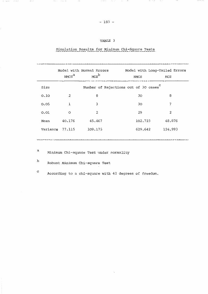
a

b

c

- 183 -

TABLE 3

Simulation Results for Minimum Chi-Square Tests

Model with Normal Errors Model with Long-Tailed Errors

NMCSa MCSb NMCS MCS

Size Number of Rejections of 30c

out cases

0.10 2 8 30 8

0.05 1 3 30 7

0.01 0 2 29 2

Mean 40.176 45.467 102.723 48.876

Variance n.1l5 109.175 629.642 124.993

Minimum Chi-square Test under normality

Robust Minimum Chi-square Test

According to a chi-square with 42 degrees of freedom.

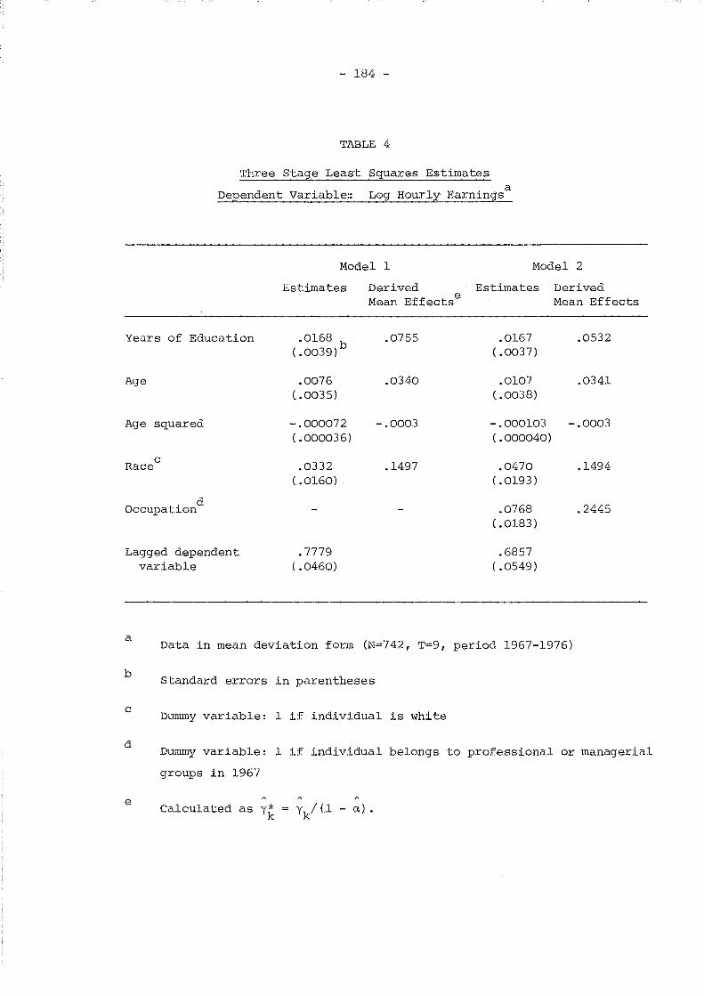
- 184 -

TABLE 4

Three Stage Least Squares Estimates

Dependent Variable:: Log Hourly Earningsa

Years of Education

Age

Age squared

Racec

occupationd

Lagged dependentvariable

Model 1 Model 2

Estimates Derived Estimates DerivedMean Effects

eMean Effects

.0168 .0755 .0167 .0532(.0039)b ( .0037)

.0076 .0340 .0107 .0341(.0035) ( .0038)

-.000072 -.0003 -.000103 -.0003( .000036) ( .000040)

.0332 .1497 .0470 .1494(.0160) (.0193)

.0768 .2445(.0183)

.7779 .6857( .0460) ( .0549)

a

b

c

d

Data in mean deviation form (N=742, T=9, period 1967-1976)

Standard errors in parentheses

Dummy variable: 1 if individual is white

Dummy variable: 1 if individual belongs to professional or managerial

groups in 1967

eCalculated as Yk a,) •

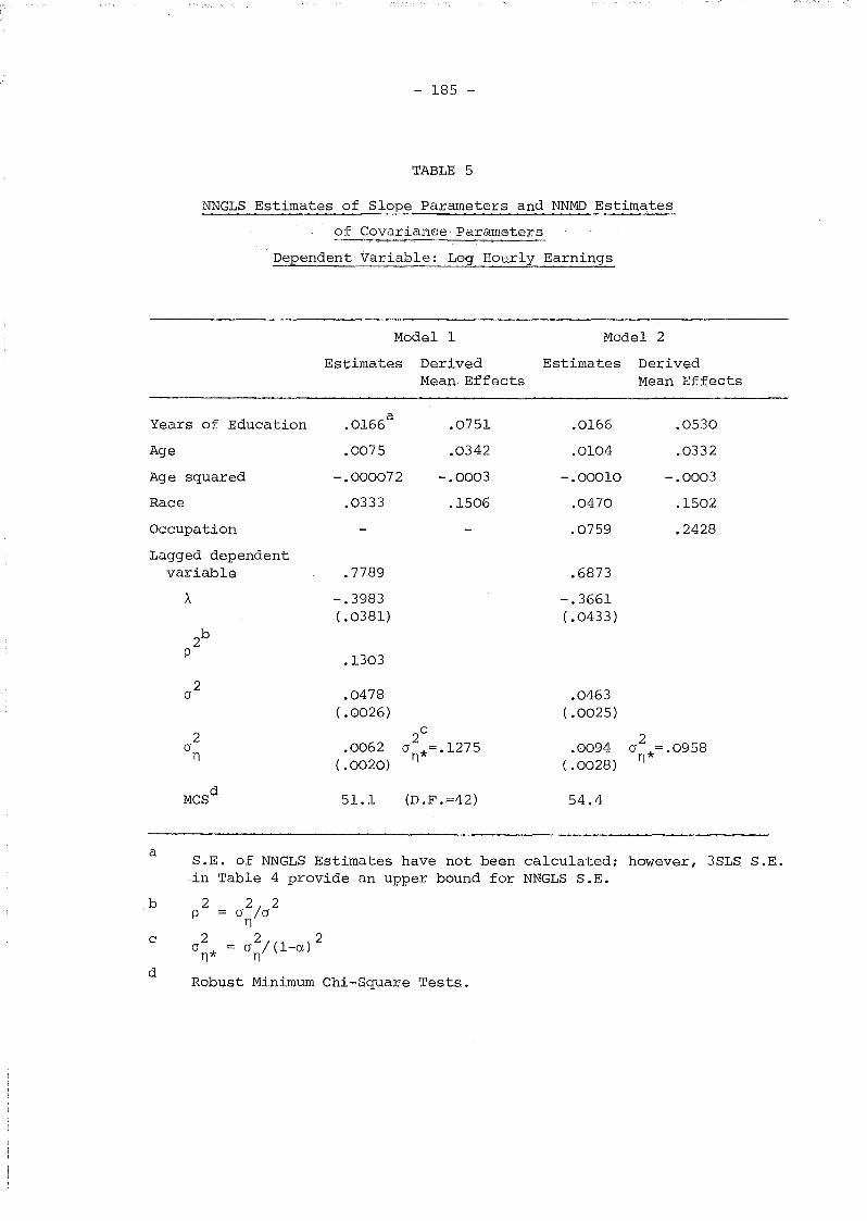
- 185 -

TABLE 5

NNGLS Estimates of; Slope J;>arameters and NNMD Estimates

of CovarianceParameters

Dependent Variable: Log Hourly Earnings

Model 1 Model 2

Estimates Derived Estimates DerivedMean Effects Mean Effects

Years of Education .0166a

.0751 .0166 .0530

Age .0075 .0342 .0104 .0332

Age squared -.000072 -.0003 -.00010 -.0003

Race .0333 .1506 .0470 .1502

Occupation .0759 .2428

Lagged dependentvariable .7789 .6873

A -.3983 -.3661( .0381) ( .0433)

2b

P .1303

2.0478 .04630

( .0026) ( .0025)

2.0062

2c

.00942

0 0 n*=·1275 o *=.0958n(.0020) ( .0028) n

MCSd

51.1 (D.F.=42) 54.4

a

b

c

d

S.E. of NNGLS Estimates have not been calculated; however, 3SLS S.E.in Table 4 provide an upper bound for NNGLS S.E.

222P = 0 /0

n0

2 = 02/(1_0\)2

n* n

Robust Minimum Chi-Square Tests.

- 186 -

TABLE 6

NGLS Estimates of Slope Parameters and NMD Estimates

of Covariance Parameters

Dependent Variable: Log Hourly Earnings

Model 1 Model 2

Estimates DerivedMean Effects

Estimates DerivedMean Effects

.7940

-.3966(.0250) a

.0153

.0073

-.000071

.0294

.0931

.0133 .0518

.0087 .0336

-.000085 -.0003

.0366 .1421

.0621 .2413

.7425

-.3663( .0285)

.1450

.0594( .0013)

.00862

C5 *=.1299( .0024) n

143.6

.0745

.0356

-.0003

.1428

(D.F .=42)

2C5 *=.1341n

140.5

.0057(.0017)

.0612( .0014)

Years of Education

2C5 n

Race

Occupation

Lagged dependentvariable

Age

Age squared

aReported S.E. of NMD estimates are only consistent under normality

bMinimum Chi-square Test under normality.

- 187 -

CONCLUSION

This thesis has presented methods of estimation and tests of

specification for dynamic econometric models from panel data when the

errors are serially correlated and the number of time periods is

small. We have derived the asymptotic properties of such estimators

in the context of general triangular systems with covariance restrictions

when normality holds and also when the errors are non-normal. Throughout,

the quasi-maximum likelihood framework has proved useful from a

theoretical point of view in organising the relevant discussion.

QML estimators are also of interest in view of their satisfactory

performance in Monte Carlo experiments, which is further supported by

the results in our empirical application using the Michigan data.

Nevertheless, there exists a full information minimum distance estimator

that is never less efficient than the QML and is strictly better when the

assumption of normality is false. Moreover, we have developed separate

MD estimators of covariance parameters and GLS estimators of slope

coefficients that are asymptotically equivalent to the full information

MD, thus providing a computationallysimpleralternative for the efficient

estimation of dynamic models from panel data.

Tests of covariance specification ought not to be based upon the

assumption of normality. Robust Wald and minimum chi-square tests as

well as appropriate probability limits for the quasi-likelihood ratio

- 188 -

test have been proposed and successfully applied in testing the

serial correlation structure to earnings equations for the US.

A comprehensive treatment of the statistical problems posed by

models with non-exogenous explanatory variables or variables with

measurement errors still has to be done. But thin will be the purpose

of future research.

- 189 -

REFERENCES

Ali, M.M. (1974): "Stochastic Ordering and Kurtosis Measure",

Journal of the American Statistical Association, 69, 543-545.

Anderson, T.W. and C. Hsiao (1981): "Estimation of Dynamic Models with

Error Components", Journal of the American Statistical Association,

76, 598-606.

Anderson, T.W. and C. Hsiao (1982): "Formulation and Estimation of

Dynamic Models Using Panel Data", Journal of Econometrics, 18, 47-82.

Arellano, M. (1983): "Estimation of Dynamic Random Effects Models with

Serially Correlated Time-Varying Errors", Paper presented at the

European Meeting of the Econometric Society, Pisa.

Arellano, M. (1984): "Testing Random Effects Specifications in Dynamic

Models for Panel Data", DEMEIC Paper, London School of Economics.

Arellano, M. (1985): "GLS and QML Estimation of Triangular Models with

Covariance Restrictions", DEMEIC Paper, London School of Economics.

Balestra, P. and M. Nerlove (1966): "Pooling Cross Section and Time Series

Data in the Estimation of a Dynamic Model: The Demand for Natural

Gas", Econometrica, 34, 585-612.

Bhargava, A., L. Franzini and W.Narendranathan (1982): "Serial Correlation

and the Fixed Effects Model", Review of Economic Studies, 49, 533-549.

Bhargava, A. and J.D. Sargan (1982): "Estimating Dynamic Random Effects

Models from Panel Data Covering Short Time Periods", Discussion

Paper no.71, University of Florida.

Bhargava, A. and J.D. Sargan (1983): "Estimating Dynamic Random Effects

Models from Panel Data Covering Short Time Periods", Econometrica,

51, 1635-1659.

- 190 -

Box, G.E.P. (1953): "Non-normality and Tests on Variances", Biometrika,

40, 318-335.

Chamberlain, G. (1980): "Analysis of Covariance with Qualitative Data",

Review of Economic Studies, 47, 225-238.

Chamberlain, G. (1982): "Multivariate Regression Models for Panel Data",

Journal of Econometrics, 18, 5-46.

Chamberlain, G. (1984): "Panel Data", in Z. Griliches and M.D. Intriligator

(eds.), Handbook of Econometrics, Volume II, Elsevier Science

Publishers.

Chiang, C.L. (1956): "On Regular Best Asymptotically Normal Estimates",

Annals of Mathematical Statistics, 27, 336-351.

Chowdhury, G. and S. Nicke11 (1982): "Individual Earnings in the U.S.

Another Look at Unionization, Schooling, Sickness and Unemployment

Using Panel Data", Discussion Paper No.141, Centre for Labour

Economics, London School of Economics.

Ferguson, T.S. (1958): "A Method of Generating Best Asymptotically Normal

Estimates with Application to the Estimation of Bacterial Densities",

Annals of Mathematical Statistics, 29, 1046-1062.

Foutz, R.V. and R.C. Srivastava (1977): "The Performance of the Likelihood

Ratio Test when the Model is Incorrect", The Annals of Statistics,

5, 1183-1194.

Hammersley, J.M. and D.C. Handscomb (1964): Monte Carlo Methods, Methuen,

London.

Hausman, J.A. and W.E. Tay10r (1981): "Panel Data and Unobservab1e

Individual Effects", Econometrica, 49, 1377-1398.

Hausman, J.A., W. Newey and W.E. Tay10r (1983): "Efficient Estimation

and Identification of Simultaneous Equation Models with Covariance

Restrictions", mimeo.

- 191 -

Hendry, D.F. (1984): "Monte Carlo Experimentation in Econometrics",

in Z. Griliches and M.D. Intriligator (eds.), Handbook of Econometrics,

Volume II, Elsevier Science Publishers.

Hendry, D.F. and R.W. Harrison (1974): "Monte Carlo Methodology and

the Small Sample Behaviour of Ordinary and Two-Stage Least Squares",

Journal of Econometrics, 2, 151-174.

Imhof, J.P. (1961): "Computing the Distribution of Quadratic Forms in

Normal Variables", Biometrika, 48, 419-426.

Kiefer, N.M. (1980): "Estimation of Fixed Effect Models for Time Series

of Cross-Sections with Arbitrary Intertemporal Covariance",

Journal of Econometrics, 14, 195-202.

Koerts, J. and A.P.J. Abrahamse (1969): On the Theory and Application of

the General Linear Model, University Press, Rotterdam.

Koopmans, T.C., H. Rubin and R.B. Leipnik (1950): "Measuring the

Equation Systems of Dynamic Economics", in T.C. Koopmans (ed.),

Statistical Inference in Dynamic Economic Models, Cowles Commission

Monograph 10, John Wiley, New York.

Lahiri, K. and P. Schmidt (1978): "On the Estimation of Triangular

Structural Systems", Econometrica, .46, 1217-1221.

Lillard, L.A. and R.J. Willis (1978): "Dynamic Aspects of Earnings

Mobility", Econometrica, 46, 985-1012.

MaCurdy, T.E. (1981): "Asymptotic Properties of Quasi-Maximum Likelihood

Estimators and Test Statistics", National Bureau of Economic Research

Technical Paper no.14.

MaCurdy, T.E. (1982): "The Use of Time Series Processes to Model the

Error Structure of Earnings in a Longitudinal Data Analysis",

Journal of Econometrics, 18, 83-114.

- 192 -

Maddala, G.S. (1971): "The Use of Variance Components Models in Pooling

Cross Section and Time Series Data", Econometrica, 39, 341-358.

Magnus, J.R. and H. Neudecker (1980): "The Elimination Matrix: Some

Lemmas and Applications", SIAM Journal of Algebraic and Discrete

Methods, 1, 422-449.

Malinvaud, E. (1970): Statistical Methods of Econometrics, North-Holland,

Amsterdam.

Mundlak, Y. (1978): "On the Pooling of Time Series and Cross Section

Data", Econometrica, 46, 69-85.

Nag Library of Computer Programs, Mark IX, Oxford University Computing

Library, Oxford.

Nerlove, M. (1967): "Experimental Evidence on the Estimation of Dynamic

Economic Relations from a Time Series of Cross-Sections",

Economic Studies Quarterly, 18, 42-74.

Nerlove, M. (1971): "Further Evidence on the Estimation of Dynamic

Economic Relations from a Time Series of Cross Sections",

Econometrica, 39, 359-382.

Nickell, S. (1981): "Biases in Dynamic Models with Fixed Effects",

Econometrica, 49, 1417-1426.

Pudney, S.E. (1979): "The Estimation and Testing of Some Error Components

Models", Discussion Paper, London School of Economics, 1979.

Rao, C.R. (1973): Linear Statistical Inference and its Applications,

Second Edition, John Wiley, New York.

Richard, J. -F. (1975): "A Note on the Information Matrix of the

Multivariate Normal Distribution", Journal of Econometrics, 3,

57-60.

- 193 -

Rothenberg, T.J. (1973): Efficient Estimation with A Priori Information,

Cowles Foundation Monograph 23, Yale University Press, New Haven.

Rothenberg, T.J. and C.T. Leenders (1964): "Efficient Estimation of

Simultaneous Equation Systems", Econometrica, 32, 57-76.

Sargan, J.D. (1964): "Three-Stage Least-Squares and Full Maximum

Likelihood Estimates", Econometrica, 32, 77-81.

Sargan, J.D. (1975): "The Identification and Estimation of Sets of

Simultaneous Stochastic Equations", London School of Economics

Econometrics Programme Discussion Paper A.l.

Sargan, J.D. and A. Bhargava (1983): "Maximum Likelihood Estimation of

Regression Models with First Order Moving Average Errors when the

Root Lies on the Unit Circle", Econometrica, 51, 799-820.

Tiao, G.C. and M.M. Ali (1971): "Analysis of Correlated Random Effects:

Linear Model with Two Random Components", Biometrika, 58, 37-51.

White, H. (1980): "Using Least Squares to Approximate Unknown Regression

Functions", International Economic Review, 21, 149-170.

Io'Jhite, H. (1980a): "A Heteroskedasticity-Consistent Covariance Matrix

Estimator and a Direct Test for Heteroskedasticity", Econometrica,

48, 817-838.

White, H. (1982): "Maximum Likelihood Estimation of Misspecified Models",

Econometrica, 50, 1-25.