1

Final ReviewEcon 240A

2

Outline The Big Picture Processes to remember ( and habits to form) for

your quantitative career (FYQC) Concepts to remember FYQC Discrete Distributions Continuous distributions Central Limit Theorem Regression

The Classical Statistical Trail

Descriptive Statistics

Inferential

Statistics

Probability Discrete Random

Variables

Discrete Probability Distributions; Moments

Binomial

Application

Rates &

Proportions

4

Where Do We Go From Here?

Regression

PropertiesAssumptions

ViolationsDiagnostics

Modeling

Probability Count ANOVA

Contingency Tables

5

Processes to Remember Exploratory Data Analysis

Distribution of the random variable Histogram Lab 1 Stem and leaf diagram Lab 1 Box plot Lab 1

Time Series plot: plot of random variable y(t) Vs. time index t

X-y plots: Y Vs. x1, y Vs. x2 etc. Diagnostic Plots

Actual, fitted and residual

6

Concepts to Remember Random Variable: takes on values with

some probability Flipping a coin

Repeated Independent Bernoulli Trials Flipping a coin twice

Random Sample Likelihood of a random sample

Prob(e1^e2 …^en) = Prob(e1)*Prob(e2)…*Prob(en)

7

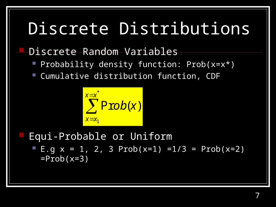
Discrete Distributions Discrete Random Variables

Probability density function: Prob(x=x*) Cumulative distribution function, CDF

Equi-Probable or Uniform E.g x = 1, 2, 3 Prob(x=1) =1/3 = Prob(x=2) =Prob(x=3)

*

1

)(Prxx

xx

xob

8

Discrete Distributions Binomial: Prob(k) = [n!/k!*(n-k)!]* pk (1-p)n-k

E(k) = n*p, Var(k) = n*p*(1-p) Simulated sample binomial random variable Lab 2 Rates and proportions

Poisson

nppnppnpVar

pnpnpE

nkp

/)1(*/)1(**)ˆ(

/*)ˆ(

/ˆ

2

9

Continuous Distributions Continuous random variables

Density function, f(x) Cumulative distribution function

Survivor function S(x*) = 1 – F(x*) Hazard function h(t) =f(t)/S(t) Cumulative hazard functin, H(t)

*

)(*)(x

dxxfxF

*

0

* )()(t

dtthtH

10

Continuous Distributions Simple moments

E(x) = mean = expected value

E(x2)

Central Moments E[x - E(x)] = 0 E[x – E(x)]2 =Var x E[x – E(x)]3 , a measure of skewness E[x – E(x)]4 , a measure of kurtosis

dxxfxxE )(*)(

11

Continuous Distributions Normal Distribution

Simulated sample random normal variable Lab 3 Approximation to the binomial, n*p>=5, n*(1-p)>=5 Standardized normal variate: z = (x-)/

Exponential Distribution Weibull Distribution

Cumulative hazard function: H(t) = (1/) t

Logarithmic transform ln H(t) = ln (1/) + lnt

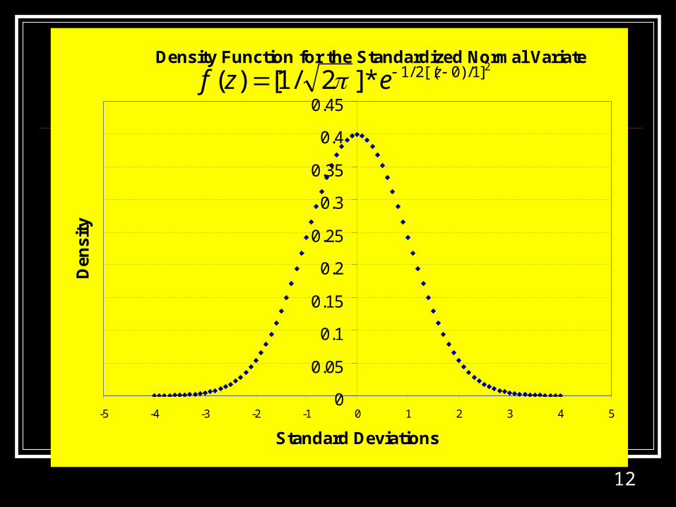
12

Density Function for the Standardized Normal Variate

0

0.05

0.1

0.15

0.2

0.25

0.3

0.35

0.4

0.45

-5 -4 -3 -2 -1 0 1 2 3 4 5

Standard Deviations

Den

sity

2]1/)0[(2/1*]2/1[)( zezf

13

Cumulative Distribution Function for a Standardized Normal Variate

0

0.1

0.2

0.3

0.4

0.5

0.6

0.7

0.8

0.9

1

-5 -4 -3 -2 -1 0 1 2 3 4 5

Standard Deviations

Pro

ba

bil

ty

14

Central Limit Theorem Sample mean,

nxxn

ii /

1

15

PopulationRandom variable xDistribution f(f ?

Sample

Sample Statistic:

),(~ 2Nx

Sample Statistic

)1/()( 2

1

2

nxxsn

ii

Pop.

16

The Sample Variance, s2

22

1

22

/*)1(

)1/(])([

sn

nxixsn

i

Is distributed 2 chi square with n-1 degrees of

freedom (text, 12.2 “inference about a population variance)(text, pp. 266-270, Chi-Squared distribution)

n

i

n

ii zxxsn

1 1

22222 /)(/)1(

17

Regression Models Statistical distributions and tests

Student’s t F Chi Square

Assumptions Pathologies

18

Regression Models Time Series

Linear trend model: y(t) =a + b*t +e(t) Lab 4 Exponential trend model: y(t) =exp[a+b*t+e(t)]

Natural logarithmic transformation ln Ln y(t) = a + b*t + e(t) Lab 4

Linear rates of change: yi = a + b*xi + ei

dy/dx = b Returns generating process:

[ri(t) – rf0] = + *[rM(t) – rf

0] + ei(t) Lab 6

19

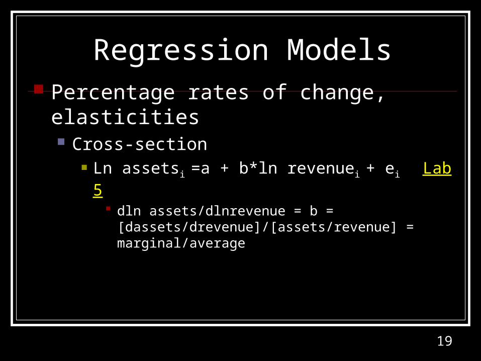
Regression Models Percentage rates of change, elasticities

Cross-section Ln assetsi =a + b*ln revenuei + ei Lab 5

dln assets/dlnrevenue = b = [dassets/drevenue]/[assets/revenue] = marginal/average

20

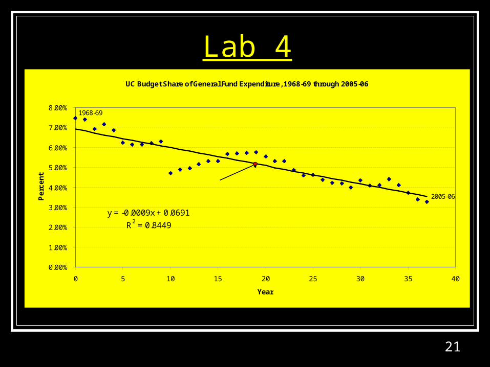
Linear Trend Model Linear trend model: y(t) =a + b*t +e(t) Lab 4

21

Lab 4UC Budget Share of General Fund Expenditure, 1968-69 through 2005-06

1968-69

2005-06

y = -0.0009x + 0.0691

R2 = 0.8449

0.00%

1.00%

2.00%

3.00%

4.00%

5.00%

6.00%

7.00%

8.00%

0 5 10 15 20 25 30 35 40

Year

Pe

rce

nt

means: 5.22%, 18.5 yr.

22

Lab FourSUMMARY OUTPUT

Regression StatisticsMultiple R 0.9191666R Square 0.8448673Adjusted R Square 0.840558Standard Error 0.0044164Observations 38

ANOVAdf SS MS F Significance F

Regression 1 0.003824089 0.003824 196.0593 3.872E-16Residual 36 0.000702171 1.95E-05Total 37 0.00452626

Coefficients Standard Error t Stat P-value Lower 95% Upper 95%Intercept 0.0690865 0.00140505 49.17012 1.32E-34 0.0662369 0.071936X Variable 1 -0.000915 6.53335E-05 -14.00212 3.87E-16 -0.001047 -0.000782

RESIDUAL OUTPUT

Observation Predicted Y Residuals1 0.0690865 0.0054338682 0.0681717 0.0057286973 0.0672569 0.0019438054 0.066342 0.005271241

t-test:H0: b=0HA: b≠0t =[ -0.000915 – 0]/0.0000653 = -14

F-test: F1,36 = [R2/1]/{[1-R2]/36} = 196= Explained Mean Square/Unexplained mean square

23

Lab 4

X Variable 1 Residual Plot

-0.015

-0.01

-0.005

0

0.005

0.01

0 10 20 30 40

X Variable 1

Re

sid

ua

ls

24

Lab 4

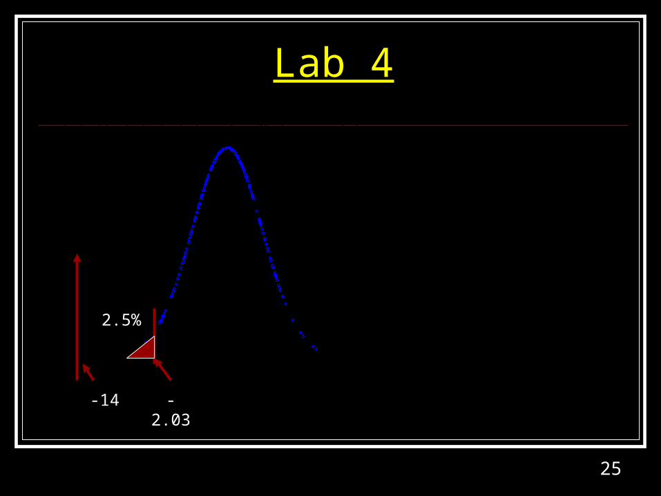
25

Lab 4

0.0

0.1

0.2

0.3

0.4

-3 -2 -1 0 1 2 3

STUDENT

DE

NS

ITY

Student's t-distribution for 36 degrees of freedom

2.5%

-14 -2.03

26

Lab Four

0

5

10

15

20

0 5 10 15

FSTAT

FD

EN

SIT

Y

F-Distribution, 1,36 degrees of freedom

4.12

5%

196

27

Exponential Trend Model Exponential trend model: y(t) =exp[a+b*t+e(t)]

Natural logarithmic transformation ln Ln y(t) = a + b*t + e(t) Lab 4

28

Lab FourUC Budget in Billions, 1968-69 through 2005-06

2005-06

y = 0.3949e0.0637x

R2 = 0.9079

0

0.5

1

1.5

2

2.5

3

3.5

4

4.5

5

0 5 10 15 20 25 30 35 40

Year

$

29

Lab FourUC Budget in Billions, 1968-69 through 2005-06

37

y = 0.0637x - 0.929

R2 = 0.9079

-1.5

-1

-0.5

0

0.5

1

1.5

2

0 5 10 15 20 25 30 35 40

Year

Lo

ga

rith

m

2005-

30

Percentage Rates of Change, Elasticities

Percentage rates of change, elasticities Cross-section

Ln assetsi =a + b*ln revenuei + ei Lab 5 dln assets/dlnrevenue = b =

[dassets/drevenue]/[assets/revenue] = marginal/average

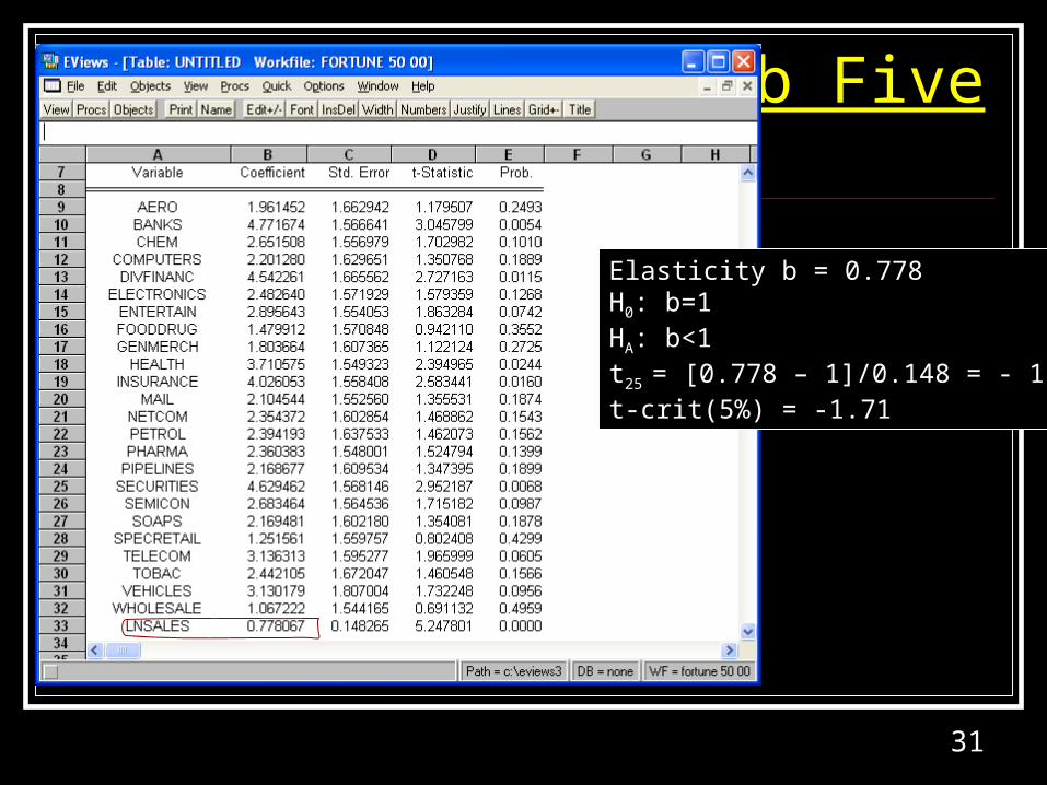
31

Lab Five

Elasticity b = 0.778H0: b=1HA: b<1t25 = [0.778 – 1]/0.148 = - 1.5t-crit(5%) = -1.71

32

Linear Rates of Change Linear rates of change: yi = a + b*xi + ei

dy/dx = b Returns generating process:

[ri(t) – rf0] = + *[rM(t) – rf

0] + ei(t) Lab 6

33

-13.35, 16.09;Ucnet,

S&Pnet

y = 1.0601x - 0.106

R2 = 0.9136

-20.00

-15.00

-10.00

-5.00

0.00

5.00

10.00

15.00

-15 -10 -5 0 5 10

Watch Excel on xy plots!

True x axis: UC Net

34

Lab SixSUMMARY OUTPUT

Regression StatisticsMultiple R 0.6362898R Square 0.4048647Adjusted R Square 0.391927Standard Error 0.0340527Observations 48

ANOVAdf SS MS F Significance F

Regression 1 0.036287438 0.036287 31.29335 1.17E-06Residual 46 0.053341113 0.00116Total 47 0.089628551

Coefficients Standard Error t Stat P-value Lower 95% Upper 95%Intercept 0.0065263 0.005659195 1.153229 0.254774 -0.00487 0.0179177X Variable 1 1.0926736 0.195327967 5.594046 1.17E-06 0.699499 1.4858484

RESIDUAL OUTPUT

Observation Predicted Y Residuals1 0.014493 -0.007183032 0.0213124 -0.0445344063 0.0297096 0.037520397

rGE = a + b*rSP500 + e

35

Lab SixX Variable 1 Line Fit Plot

-0.1

0

0.1

0.2

-0.1 -0.05 0 0.05 0.1

X Variable 1

Y

Y

Predicted Y

36

Lab Six

X Variable 1 Residual Plot

-0.1

0

0.1

0.2

-0.1 -0.05 0 0.05 0.1

X Variable 1

Re

sid

ua

ls

37

View/Residual tests/Histogram-Normality Test

38

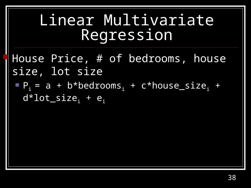
Linear Multivariate Regression House Price, # of bedrooms, house size, lot

size Pi = a + b*bedroomsi + c*house_sizei + d*lot_sizei + ei

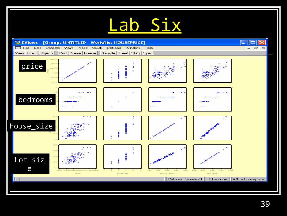
39

Lab Six

price

bedrooms

House_size

Lot_size

40

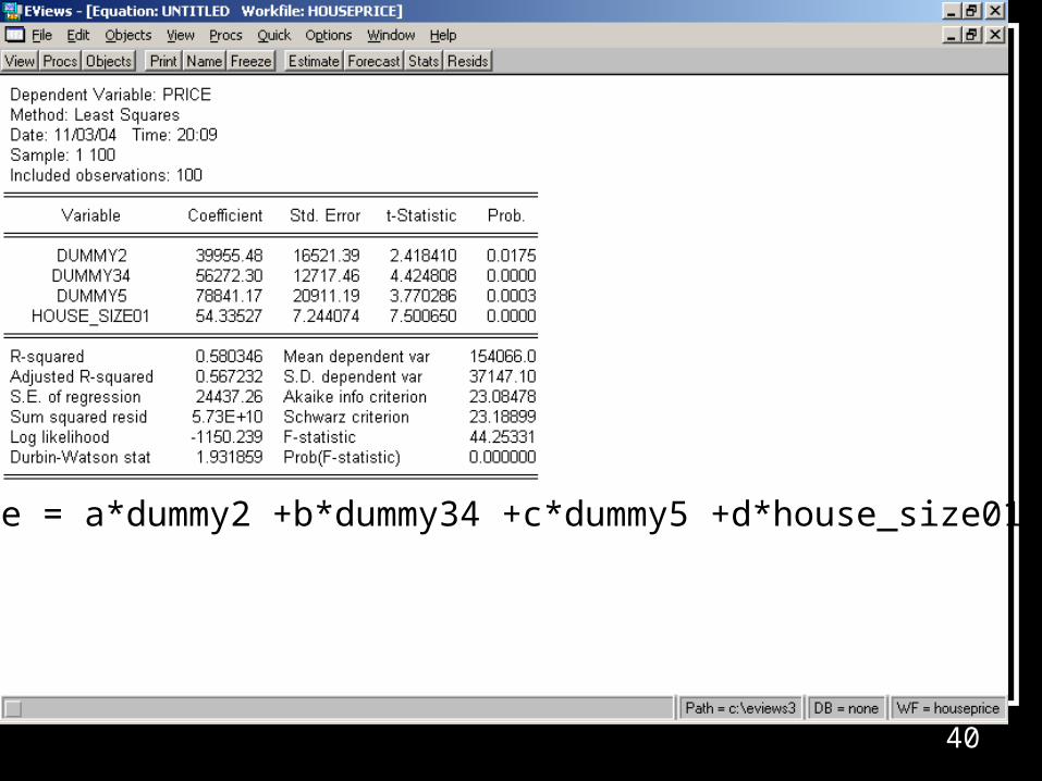
Price = a*dummy2 +b*dummy34 +c*dummy5 +d*house_size01 +e

41

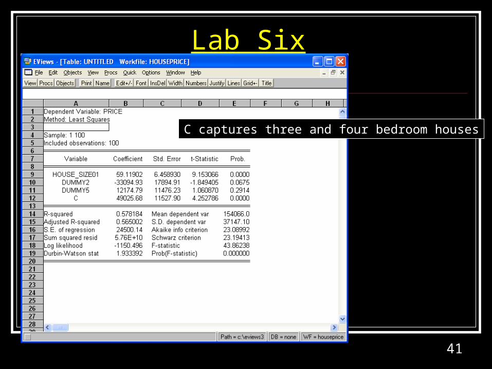
Lab Six

C captures three and four bedroom houses

42

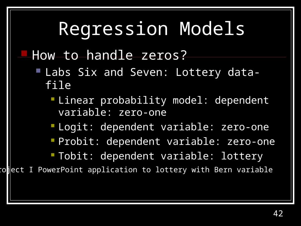
Regression Models How to handle zeros?

Labs Six and Seven: Lottery data-file Linear probability model: dependent variable:

zero-one Logit: dependent variable: zero-one Probit: dependent variable: zero-one Tobit: dependent variable: lottery

See Project I PowerPoint application to lottery with Bern variable

43

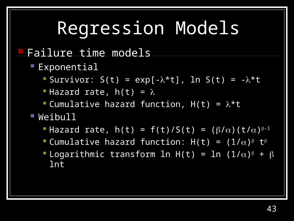
Regression Models Failure time models

Exponential Survivor: S(t) = exp[-*t], ln S(t) = -*t Hazard rate, h(t) = Cumulative hazard function, H(t) = *t

Weibull Hazard rate, h(t) = f(t)/S(t) = (/)(t/)-1

Cumulative hazard function: H(t) = (1/) t

Logarithmic transform ln H(t) = ln (1/) + lnt

44

Applications: Discrete Distributions Binomial

Equi-probable or uniform

Poisson

Rates & proportions, small samples, ex. Voting polls

If I asked a question every day, without replacement, what is the chance I will ask you a question today?

Approximate the binomial where p→0

45

Aplications: Discrete Distributions Multinomial More than two

outcomes, ex each face of the die or 6 outcomes

46

Applications: Continuous Distributions Normal

Equi-probable or uniform

Students t

Rates & proportions, np>5, n(1-p)>5; tests about population means given 2

Tests about population means, 2 not known; test regression parameter = 0

47

Applications: Continuous Distributions F

Ch-Square, 2

Regression: ratio of explained mean square to unexplained mean square, i.e. R2/k÷(1-R2)/(n-k); test dropping 2 or more variables (Wald test)

Contingency Table analysis; Likelihood ratio tests (Wald test)

48

Applications: Continuous Distributions Exponential

Weibull

Failure (survival) time with constant hazard rate

Failure time analysis, test whether hazard rate is constant or increasing or decreasing

49

Labs 7, 8, 9 Lab 7 Failure Time Analysis

Lab 8 Contingency Table Analysis

Lab 9 One-Way and Two-Way ANOVA