1

Box 1.1: Highlights of this report

Due to the record high sea surface temperature anomalies in both the northeast Pacific and the region off Baja California and the development of the third largest El Niño this century, for the 2014 – 2015 period the California Current Ecosystem can be classified as lower productivity at almost every trophic level. Oceanographic conditions, represented by MEI, PDO and NPGO indices, indicated warmer conditions throughout.

The northern copepod index decreased off of Newport, indicating lower energy content for higher trophic levels.

High energy forage species were at low levels, while forage species with low and intermediate energy content were patchy; catches of young of the year rockfish and market squid were very high South of Cape Mendocino.

Pacific salmon faced additional stresses due to drought, warm weather, warm streams and 95% below-normal snow-water equivalent storage.

Unusual mortality events for California sea lions and Guadalupe Fur Seals, as well as an unusually large, coast-wide common murre wreck, are further evidence of overall lower productivity in the California Current Ecosystem.

Commercial fishing landings remained high, driven mainly by landings of Pacific hake and coastal pelagic species.

Newly developed indicators of coastal community vulnerability show that fishery-dependent communities experienced increasing socioeconomic vulnerability from 2000 to 2010.

CALIFORNIA CURRENT INTEGRATED ECOSYSTEM ASSESSMENT (CCIEA) STATE OF THE CALIFORNIA CURRENT REPORT, 2016

A report of the NOAA CCIEA Team to the Pacific Fishery Management Council, March 9, 2016. Editors: Dr. Toby Garfield (SWFSC) and Dr. Chris Harvey (NWFSC)

1 INTRODUCTION

Section 1.4 of the 2013 Fishery Ecosystem Plan (FEP) outlines a reporting process wherein NOAA provides the Council with a yearly update on the state of the California Current Ecosystem (CCE), as derived from environmental, biological and socio-economic indicators. NOAA’s California Current Integrated Ecosystem Assessment (CCIEA) team is responsible for this report. This marks our 4th such report, with prior reports in 2012, 2014 and 2015.

The highlights of this report are summarized in Box 1.1. Sections below provide greater detail. In addition, a list of supplemental materials is provided at the end of this document, in response to previous requests from Council members or the Scientific and Statistical Committee (SSC) to provide additional information, or to clarify details within this short report.

Agenda Item D.1.a NMFS Report 1

March 2016

2

1.1 NOTES ON INTERPRETING TIME SERIES FIGURES

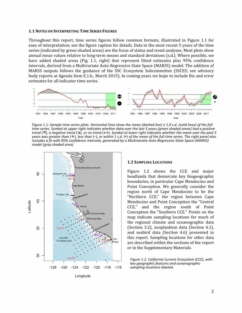
Throughout this report, time series figures follow common formats, illustrated in Figure 1.1 for ease of interpretation; see the figure caption for details. Data in the most recent 5 years of the time series (indicated by green shaded areas) are the focus of status and trend analyses. Most plots show annual mean values relative to long-term means and standard deviations (s.d.). Where possible, we have added shaded areas (Fig. 1.1, right) that represent fitted estimates plus 95% confidence intervals, derived from a Multivariate Auto-Regressive State Space (MARSS) model. The addition of MARSS outputs follows the guidance of the SSC Ecosystem Subcommittee (SSCES; see advisory body reports at Agenda Item E.1.b., March 2015). In coming years we hope to include fits and error estimates for all indicator time series.

1.2 SAMPLING LOCATIONS

Figure 1.2 shows the CCE and major headlands that demarcate key biogeographic boundaries, in particular Cape Mendocino and Point Conception. We generally consider the region north of Cape Mendocino to be the “Northern CCE,” the region between Cape Mendocino and Point Conception the “Central CCE,” and the region south of Point Conception the “Southern CCE.” Points on the map indicate sampling locations for much of the regional climate and oceanographic data (Section 3.2), zooplankton data (Section 4.1), and seabird data (Section 4.6) presented in this report. Sampling locations for other data are described within the sections of the report or in the Supplementary Materials.

Figure 1.1: Sample time series plots. Horizontal lines show the mean (dashed line) ± 1.0 s.d. (solid lines) of the full time series. Symbol at upper right indicates whether data over the last 5 years (green shaded areas) had a positive trend (), a negative trend (), or no trend (↔). Symbol at lower right indicates whether the mean over the past 5 years was greater than (), less than (–), or within 1 s.d. () of the mean of the full time series. The right panel also includes a fit with 95% confidence intervals, generated by a Multivariate Auto-Regressive State Space (MARSS) model (gray shaded area).

Figure 1.2. California Current Ecosystem (CCE), with key geographic features and oceanographic sampling locations labeled.

3

2. CONCEPTUAL MODELS OF THE CALIFORNIA CURRENT

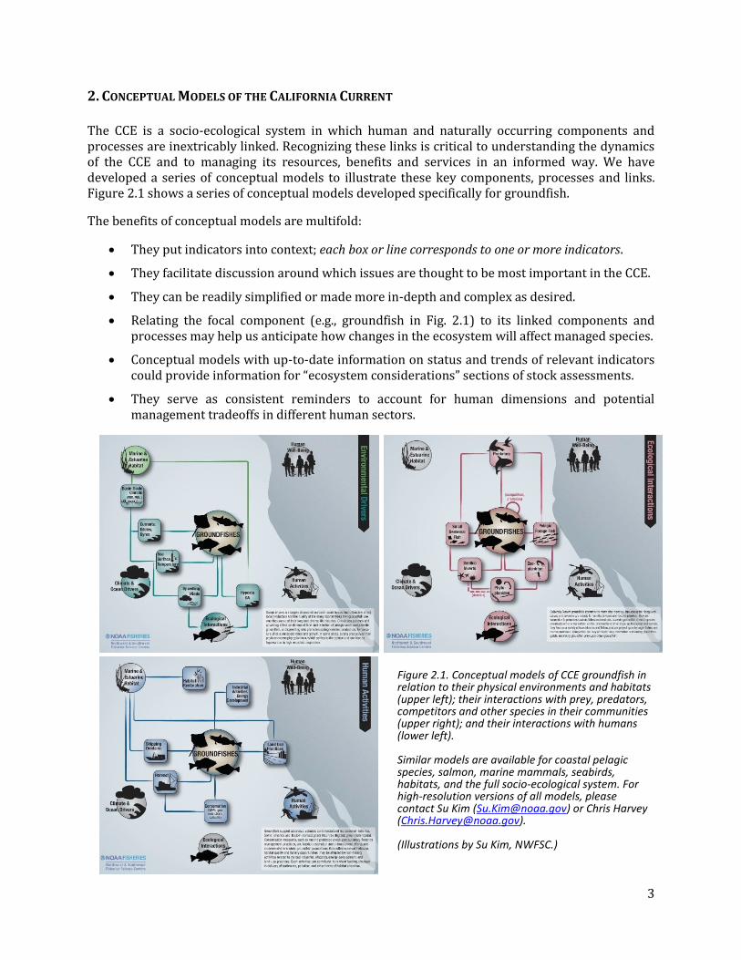
The CCE is a socio-ecological system in which human and naturally occurring components and processes are inextricably linked. Recognizing these links is critical to understanding the dynamics of the CCE and to managing its resources, benefits and services in an informed way. We have developed a series of conceptual models to illustrate these key components, processes and links. Figure 2.1 shows a series of conceptual models developed specifically for groundfish.

The benefits of conceptual models are multifold:

They put indicators into context; each box or line corresponds to one or more indicators.

They facilitate discussion around which issues are thought to be most important in the CCE.

They can be readily simplified or made more in-depth and complex as desired.

Relating the focal component (e.g., groundfish in Fig. 2.1) to its linked components and processes may help us anticipate how changes in the ecosystem will affect managed species.

Conceptual models with up-to-date information on status and trends of relevant indicators could provide information for “ecosystem considerations” sections of stock assessments.

They serve as consistent reminders to account for human dimensions and potential management tradeoffs in different human sectors.

Figure 2.1. Conceptual models of CCE groundfish in relation to their physical environments and habitats (upper left); their interactions with prey, predators, competitors and other species in their communities (upper right); and their interactions with humans (lower left). Similar models are available for coastal pelagic species, salmon, marine mammals, seabirds, habitats, and the full socio-ecological system. For high-resolution versions of all models, please contact Su Kim (Su.Kim@noaa.gov) or Chris Harvey (Chris.Harvey@noaa.gov). (Illustrations by Su Kim, NWFSC.)

4

3 CLIMATE AND OCEAN DRIVERS

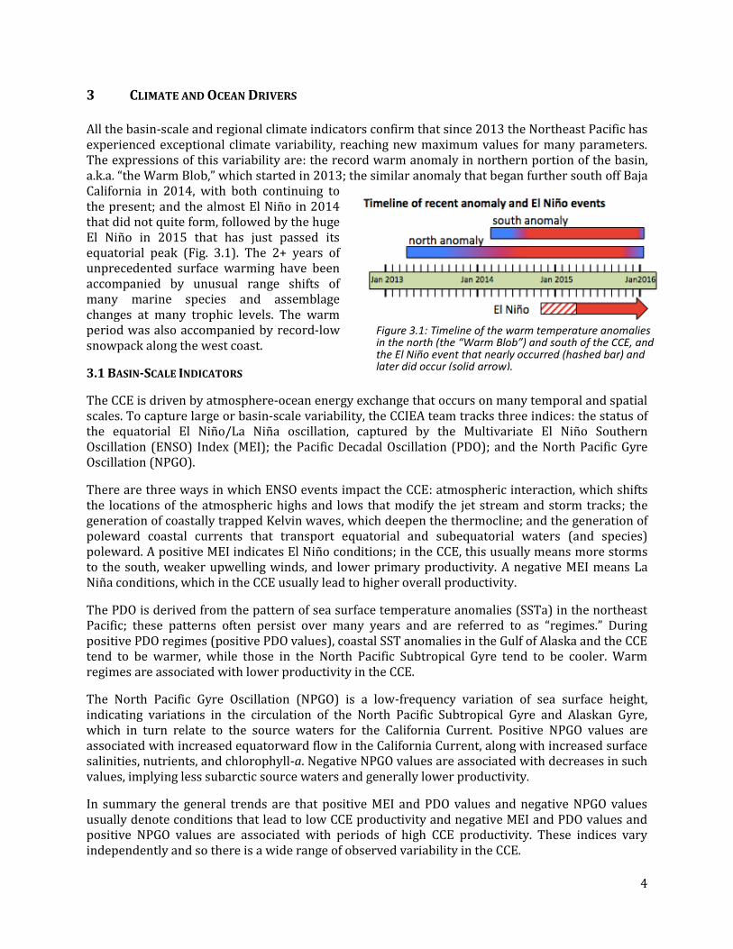
All the basin-scale and regional climate indicators confirm that since 2013 the Northeast Pacific has experienced exceptional climate variability, reaching new maximum values for many parameters. The expressions of this variability are: the record warm anomaly in northern portion of the basin, a.k.a. “the Warm Blob,” which started in 2013; the similar anomaly that began further south off Baja California in 2014, with both continuing to the present; and the almost El Niño in 2014 that did not quite form, followed by the huge El Niño in 2015 that has just passed its equatorial peak (Fig. 3.1). The 2+ years of unprecedented surface warming have been accompanied by unusual range shifts of many marine species and assemblage changes at many trophic levels. The warm period was also accompanied by record-low snowpack along the west coast.

3.1 BASIN-SCALE INDICATORS

The CCE is driven by atmosphere-ocean energy exchange that occurs on many temporal and spatial scales. To capture large or basin-scale variability, the CCIEA team tracks three indices: the status of the equatorial El Niño/La Niña oscillation, captured by the Multivariate El Niño Southern Oscillation (ENSO) Index (MEI); the Pacific Decadal Oscillation (PDO); and the North Pacific Gyre Oscillation (NPGO).

There are three ways in which ENSO events impact the CCE: atmospheric interaction, which shifts the locations of the atmospheric highs and lows that modify the jet stream and storm tracks; the generation of coastally trapped Kelvin waves, which deepen the thermocline; and the generation of poleward coastal currents that transport equatorial and subequatorial waters (and species) poleward. A positive MEI indicates El Niño conditions; in the CCE, this usually means more storms to the south, weaker upwelling winds, and lower primary productivity. A negative MEI means La Niña conditions, which in the CCE usually lead to higher overall productivity.

The PDO is derived from the pattern of sea surface temperature anomalies (SSTa) in the northeast Pacific; these patterns often persist over many years and are referred to as “regimes.” During positive PDO regimes (positive PDO values), coastal SST anomalies in the Gulf of Alaska and the CCE tend to be warmer, while those in the North Pacific Subtropical Gyre tend to be cooler. Warm regimes are associated with lower productivity in the CCE.

The North Pacific Gyre Oscillation (NPGO) is a low-frequency variation of sea surface height, indicating variations in the circulation of the North Pacific Subtropical Gyre and Alaskan Gyre, which in turn relate to the source waters for the California Current. Positive NPGO values are associated with increased equatorward flow in the California Current, along with increased surface salinities, nutrients, and chlorophyll-a. Negative NPGO values are associated with decreases in such values, implying less subarctic source waters and generally lower productivity.

In summary the general trends are that positive MEI and PDO values and negative NPGO values usually denote conditions that lead to low CCE productivity and negative MEI and PDO values and positive NPGO values are associated with periods of high CCE productivity. These indices vary independently and so there is a wide range of observed variability in the CCE.

Figure 3.1: Timeline of the warm temperature anomalies in the north (the “Warm Blob”) and south of the CCE, and the El Niño event that nearly occurred (hashed bar) and later did occur (solid arrow).

5

3.1.1 BASIN-SCALE PROCESSES IN THE CCE, 2013-2015

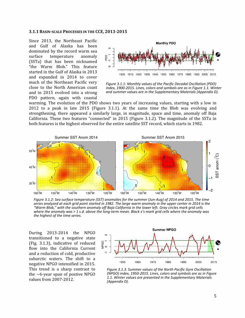
Since 2013, the Northeast Pacific and Gulf of Alaska has been dominated by the record warm sea surface temperature anomaly (SSTa) that has been nicknamed “the Warm Blob.” This feature started in the Gulf of Alaska in 2013 and expanded in 2014 to cover much of the Northeast Pacific very close to the North American coast and in 2015 evolved into a strong PDO pattern, again with coastal warming. The evolution of the PDO shows two years of increasing values, starting with a low in 2012 to a peak in late 2015 (Figure 3.1.1). At the same time the Blob was evolving and strengthening, there appeared a similarly large, in magnitude, space and time, anomaly off Baja California. These two features “connected” in 2015 (Figure 3.1.2). The magnitude of the SSTa in both features is the highest observed for the entire satellite SST record, which starts in 1982.

During 2013-2014 the NPGO transitioned to a negative state (Fig. 3.1.3), indicative of reduced flow into the California Current and a reduction of cold, productive subarctic waters. The shift to a negative NPGO intensified in 2015. This trend is a sharp contrast to the ~6-year span of postive NPGO values from 2007-2012.

Figure 3.1.1: Monthly values of the Pacific Decadal Oscillation (PDO) index, 1900-2015. Lines, colors and symbols are as in Figure 1.1. Winter and summer values are in the Supplementary Materials (Appendix D).

Figure 3.1.2: Sea surface temperature (SST) anomalies for the summer (Jun-Aug) of 2014 and 2015. The time series analyzed at each grid point started in 1982. The large warm anomaly in the upper center in 2014 is the “Warm Blob,” with the southern anomaly off Baja California in the lower left. Gray circles mark grid cells where the anomaly was > 1 s.d. above the long-term mean. Black x’s mark grid cells where the anomaly was the highest of the time series.

Figure 3.1.3. Summer values of the North Pacific Gyre Oscillation (NPGO) index, 1950-2015. Lines, colors and symbols are as in Figure 1.1. Winter values are presented in the Supplementary Materials (Appendix D).

6

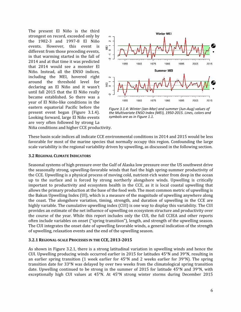
The present El Niño is the third strongest on record, exceeded only by the 1982-3 and 1997-8 El Niño events. However, this event is different from those preceding events, in that warming started in the fall of 2014 and at that time it was predicted that 2014 would see a monster El Niño. Instead, all the ENSO indices, including the MEI, hovered right around the threshold level for declaring an El Niño and it wasn’t until fall 2015 that the El Niño really became established. So there was a year of El Niño-like conditions in the eastern equatorial Pacific before the present event began (Figure 3.1.4). Looking forward, large El Niño events are very often followed by strong La Niña conditions and higher CCE productivity.

These basin scale indices all indicate CCE environmental conditions in 2014 and 2015 would be less favorable for most of the marine species that normally occupy this region. Confounding the large scale variability is the regional variability driven by upwelling, as discussed in the following section.

3.2 REGIONAL CLIMATE INDICATORS

Seasonal systems of high pressure over the Gulf of Alaska low pressure over the US southwest drive the seasonally strong, upwelling-favorable winds that fuel the high spring-summer productivity of the CCE. Upwelling is a physical process of moving cold, nutrient-rich water from deep in the ocean up to the surface and is forced by strong northerly alongshore winds. Upwelling is critically important to productivity and ecosystem health in the CCE, as it is local coastal upwelling that allows the primary production at the base of the food web. The most common metric of upwelling is the Bakun Upwelling Index (UI), which is a measure of the magnitude of upwelling anywhere along the coast. The alongshore variation, timing, strength, and duration of upwelling in the CCE are highly variable. The cumulative upwelling index (CUI) is one way to display this variability. The CUI provides an estimate of the net influence of upwelling on ecosystem structure and productivity over the course of the year. While this report includes only the CUI, the full CCIEA and other reports often include variables on onset (“spring transition”), length, and strength of the upwelling season. The CUI integrates the onset date of upwelling favorable winds, a general indication of the strength of upwelling, relaxation events and the end of the upwelling season.

3.2.1 REGIONAL-SCALE PROCESSES IN THE CCE, 2013-2015

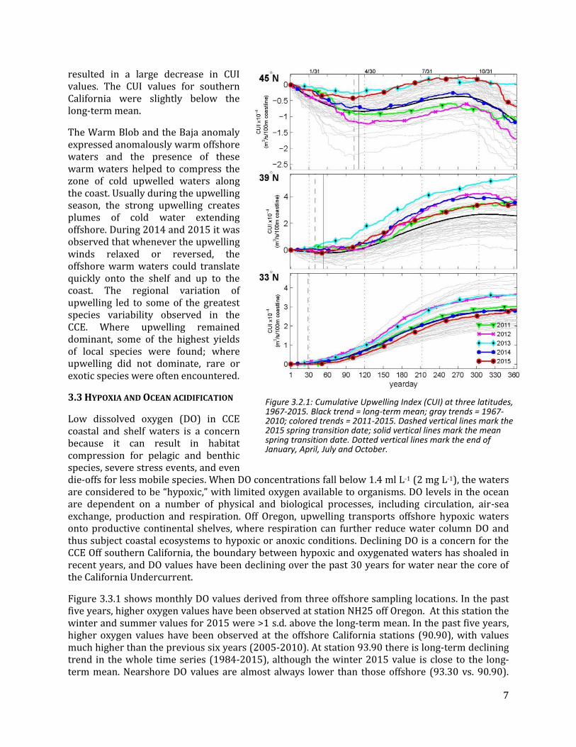
As shown in Figure 3.2.1, there is a strong latitudinal variation in upwelling winds and hence the CUI. Upwelling producing winds occurred earlier in 2015 for latitudes 45°N and 39°N, resulting in an earlier spring transition (1 week earlier for 45°N and 2 weeks earlier for 39°N). The spring transition date for 33°N was delayed by over two weeks from the climatological spring transition date. Upwelling continued to be strong in the summer of 2015 for latitude 45°N and 39°N, with exceptionally high CUI values at 45°N. At 45°N strong winter storms during December 2015

Figure 3.1.4: Winter (Jan-Mar) and summer (Jun-Aug) values of the Multivariate ENSO Index (MEI), 1950-2015. Lines, colors and symbols are as in Figure 1.1.

7

resulted in a large decrease in CUI values. The CUI values for southern California were slightly below the long-term mean.

The Warm Blob and the Baja anomaly expressed anomalously warm offshore waters and the presence of these warm waters helped to compress the zone of cold upwelled waters along the coast. Usually during the upwelling season, the strong upwelling creates plumes of cold water extending offshore. During 2014 and 2015 it was observed that whenever the upwelling winds relaxed or reversed, the offshore warm waters could translate quickly onto the shelf and up to the coast. The regional variation of upwelling led to some of the greatest species variability observed in the CCE. Where upwelling remained dominant, some of the highest yields of local species were found; where upwelling did not dominate, rare or exotic species were often encountered.

3.3 HYPOXIA AND OCEAN ACIDIFICATION

Low dissolved oxygen (DO) in CCE coastal and shelf waters is a concern because it can result in habitat compression for pelagic and benthic species, severe stress events, and even die-offs for less mobile species. When DO concentrations fall below 1.4 ml L-1 (2 mg L-1), the waters are considered to be “hypoxic,” with limited oxygen available to organisms. DO levels in the ocean are dependent on a number of physical and biological processes, including circulation, air-sea exchange, production and respiration. Off Oregon, upwelling transports offshore hypoxic waters onto productive continental shelves, where respiration can further reduce water column DO and thus subject coastal ecosystems to hypoxic or anoxic conditions. Declining DO is a concern for the CCE Off southern California, the boundary between hypoxic and oxygenated waters has shoaled in recent years, and DO values have been declining over the past 30 years for water near the core of the California Undercurrent.

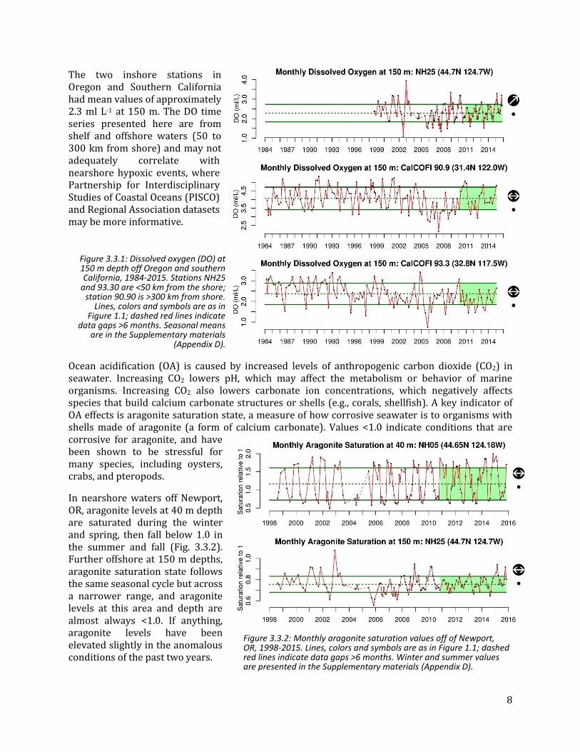
Figure 3.3.1 shows monthly DO values derived from three offshore sampling locations. In the past five years, higher oxygen values have been observed at station NH25 off Oregon. At this station the winter and summer values for 2015 were >1 s.d. above the long-term mean. In the past five years, higher oxygen values have been observed at the offshore California stations (90.90), with values much higher than the previous six years (2005-2010). At station 93.90 there is long-term declining trend in the whole time series (1984-2015), although the winter 2015 value is close to the long-term mean. Nearshore DO values are almost always lower than those offshore (93.30 vs. 90.90).

Figure 3.2.1: Cumulative Upwelling Index (CUI) at three latitudes, 1967-2015. Black trend = long-term mean; gray trends = 1967-2010; colored trends = 2011-2015. Dashed vertical lines mark the 2015 spring transition date; solid vertical lines mark the mean spring transition date. Dotted vertical lines mark the end of January, April, July and October.

8

Figure 3.3.1: Dissolved oxygen (DO) at 150 m depth off Oregon and southern California, 1984-2015. Stations NH25

and 93.30 are <50 km from the shore; station 90.90 is >300 km from shore.

Lines, colors and symbols are as in Figure 1.1; dashed red lines indicate

data gaps >6 months. Seasonal means are in the Supplementary materials

(Appendix D).

The two inshore stations in Oregon and Southern California had mean values of approximately 2.3 ml L-1 at 150 m. The DO time series presented here are from shelf and offshore waters (50 to 300 km from shore) and may not adequately correlate with nearshore hypoxic events, where Partnership for Interdisciplinary Studies of Coastal Oceans (PISCO) and Regional Association datasets may be more informative.

Ocean acidification (OA) is caused by increased levels of anthropogenic carbon dioxide (CO2) in seawater. Increasing CO2 lowers pH, which may affect the metabolism or behavior of marine organisms. Increasing CO2 also lowers carbonate ion concentrations, which negatively affects species that build calcium carbonate structures or shells (e.g., corals, shellfish). A key indicator of OA effects is aragonite saturation state, a measure of how corrosive seawater is to organisms with shells made of aragonite (a form of calcium carbonate). Values <1.0 indicate conditions that are corrosive for aragonite, and have been shown to be stressful for many species, including oysters, crabs, and pteropods.

In nearshore waters off Newport, OR, aragonite levels at 40 m depth are saturated during the winter and spring, then fall below 1.0 in the summer and fall (Fig. 3.3.2). Further offshore at 150 m depths, aragonite saturation state follows the same seasonal cycle but across a narrower range, and aragonite levels at this area and depth are almost always <1.0. If anything, aragonite levels have been elevated slightly in the anomalous conditions of the past two years.

Figure 3.3.2: Monthly aragonite saturation values off of Newport, OR, 1998-2015. Lines, colors and symbols are as in Figure 1.1; dashed red lines indicate data gaps >6 months. Winter and summer values are presented in the Supplementary materials (Appendix D).

9

3.4 HYDROLOGIC INDICATORS

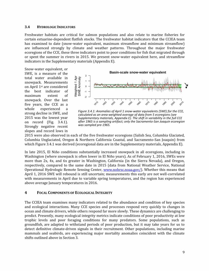
Freshwater habitats are critical for salmon populations and also relate to marine fisheries for certain estuarine-dependent flatfish stocks. The freshwater habitat indicators that the CCIEA team has examined to date (snow-water equivalent, maximum streamflow and minimum streamflow) are influenced strongly by climate and weather patterns. Throughout the major freshwater ecoregions of the CCE, these three indicators point to poor conditions for fish that migrated through or spent the summer in rivers in 2015. We present snow-water equivalent here, and streamflow indicators in the Supplementary materials (Appendix E).

Snow-water equivalent, or SWE, is a measure of the total water available in snowpack. Measurements on April 1st are considered the best indicator of maximum extent of snowpack. Over the last five years, the CCE as a whole experienced a strong decline in SWE, and 2015 was the lowest year on record (Fig. 3.4.1). Strongly negative recent slopes and record lows in 2015 were also observed in each of the five freshwater ecoregions (Salish Sea, Columbia Glaciated, Columbia Unglaciated, Oregon & Northern California Coastal, and Sacramento-San Joaquin) from which Figure 3.4.1 was derived (ecoregional data are in the Supplementary materials, Appendix E).

In late 2015, El Niño conditions substantially increased snowpack in all ecoregions, including in Washington (where snowpack is often lower in El Niño years). As of February 1, 2016, SWEs were more than 2x, 4x, and 6x greater in Washington, California (in the Sierra Nevada), and Oregon, respectively, compared to the same date in 2015 (data from National Weather Service, National Operational Hydrologic Remote Sensing Center, www.nohrsc.noaa.gov/). Whether this means that April 1, 2016 SWE will rebound is still uncertain; measurements this early are not well-correlated with measurements in April due to variable spring temperatures, and the region has experienced above average January temperatures in 2016.

4 FOCAL COMPONENTS OF ECOLOGICAL INTEGRITY

The CCIEA team examines many indicators related to the abundance and condition of key species and ecological interactions. Many CCE species and processes respond very quickly to changes in ocean and climate drivers, while others respond far more slowly. These dynamics are challenging to predict. Presently, many ecological integrity metrics indicate conditions of poor productivity at low trophic levels and poor foraging conditions for many predators. Some populations, such as groundfish, are adapted to withstand periods of poor production, but it may take years for us to detect definitive climate-driven signals in their recruitment. Other populations, including marine mammals and seabirds, are experiencing major mortality anomalies coincident with the climate shifts outlined above in Section 3.

Figure 3.4.1: Anomalies of April 1 snow-water equivalents (SWE) for the CCE, calculated as an area-weighted average of data from 5 ecoregions (see Supplementary materials, Appendix E). The shift in variability in the full CCE after 1965 is a sampling artifact; only the Sacramento-San Joaquin ecoregion was sampled pre-1965.

Basin-scale snow-water equivalent

10

4.1 NORTHERN COPEPOD BIOMASS ANOMALY

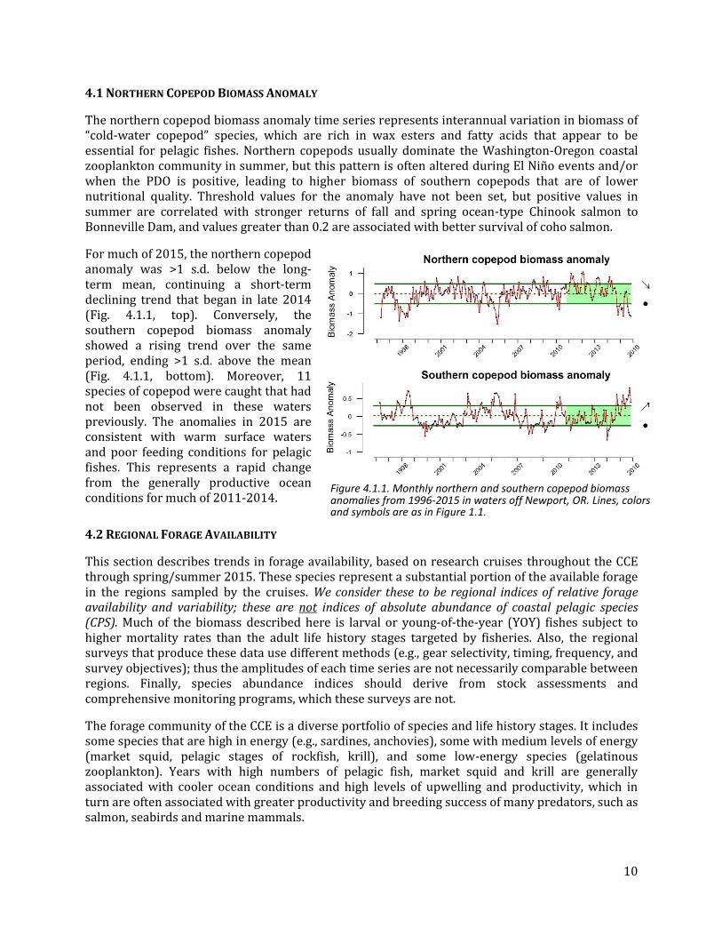
The northern copepod biomass anomaly time series represents interannual variation in biomass of “cold-water copepod” species, which are rich in wax esters and fatty acids that appear to be essential for pelagic fishes. Northern copepods usually dominate the Washington-Oregon coastal zooplankton community in summer, but this pattern is often altered during El Niño events and/or when the PDO is positive, leading to higher biomass of southern copepods that are of lower nutritional quality. Threshold values for the anomaly have not been set, but positive values in summer are correlated with stronger returns of fall and spring ocean-type Chinook salmon to Bonneville Dam, and values greater than 0.2 are associated with better survival of coho salmon.

For much of 2015, the northern copepod anomaly was >1 s.d. below the long-term mean, continuing a short-term declining trend that began in late 2014 (Fig. 4.1.1, top). Conversely, the southern copepod biomass anomaly showed a rising trend over the same period, ending >1 s.d. above the mean (Fig. 4.1.1, bottom). Moreover, 11 species of copepod were caught that had not been observed in these waters previously. The anomalies in 2015 are consistent with warm surface waters and poor feeding conditions for pelagic fishes. This represents a rapid change from the generally productive ocean conditions for much of 2011-2014.

4.2 REGIONAL FORAGE AVAILABILITY

This section describes trends in forage availability, based on research cruises throughout the CCE through spring/summer 2015. These species represent a substantial portion of the available forage in the regions sampled by the cruises. We consider these to be regional indices of relative forage availability and variability; these are not indices of absolute abundance of coastal pelagic species (CPS). Much of the biomass described here is larval or young-of-the-year (YOY) fishes subject to higher mortality rates than the adult life history stages targeted by fisheries. Also, the regional surveys that produce these data use different methods (e.g., gear selectivity, timing, frequency, and survey objectives); thus the amplitudes of each time series are not necessarily comparable between regions. Finally, species abundance indices should derive from stock assessments and comprehensive monitoring programs, which these surveys are not.

The forage community of the CCE is a diverse portfolio of species and life history stages. It includes some species that are high in energy (e.g., sardines, anchovies), some with medium levels of energy (market squid, pelagic stages of rockfish, krill), and some low-energy species (gelatinous zooplankton). Years with high numbers of pelagic fish, market squid and krill are generally associated with cooler ocean conditions and high levels of upwelling and productivity, which in turn are often associated with greater productivity and breeding success of many predators, such as salmon, seabirds and marine mammals.

Figure 4.1.1. Monthly northern and southern copepod biomass anomalies from 1996-2015 in waters off Newport, OR. Lines, colors and symbols are as in Figure 1.1.

11

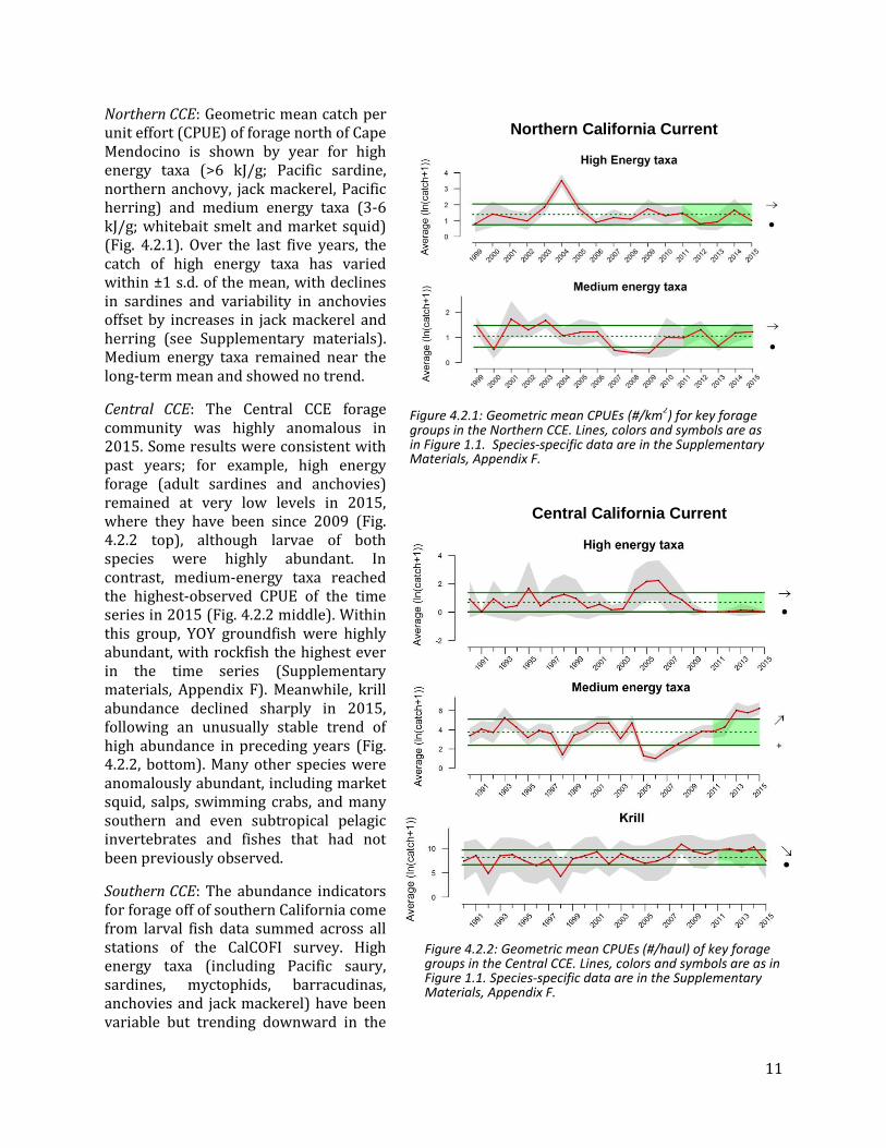
Northern CCE: Geometric mean catch per unit effort (CPUE) of forage north of Cape Mendocino is shown by year for high energy taxa (>6 kJ/g; Pacific sardine, northern anchovy, jack mackerel, Pacific herring) and medium energy taxa (3-6 kJ/g; whitebait smelt and market squid) (Fig. 4.2.1). Over the last five years, the catch of high energy taxa has varied within ±1 s.d. of the mean, with declines in sardines and variability in anchovies offset by increases in jack mackerel and herring (see Supplementary materials). Medium energy taxa remained near the long-term mean and showed no trend.

Central CCE: The Central CCE forage community was highly anomalous in 2015. Some results were consistent with past years; for example, high energy forage (adult sardines and anchovies) remained at very low levels in 2015, where they have been since 2009 (Fig. 4.2.2 top), although larvae of both species were highly abundant. In contrast, medium-energy taxa reached the highest-observed CPUE of the time series in 2015 (Fig. 4.2.2 middle). Within this group, YOY groundfish were highly abundant, with rockfish the highest ever in the time series (Supplementary materials, Appendix F). Meanwhile, krill abundance declined sharply in 2015, following an unusually stable trend of high abundance in preceding years (Fig. 4.2.2, bottom). Many other species were anomalously abundant, including market squid, salps, swimming crabs, and many southern and even subtropical pelagic invertebrates and fishes that had not been previously observed.

Southern CCE: The abundance indicators for forage off of southern California come from larval fish data summed across all stations of the CalCOFI survey. High energy taxa (including Pacific saury, sardines, myctophids, barracudinas, anchovies and jack mackerel) have been variable but trending downward in the

Central California Current

Figure 4.2.2: Geometric mean CPUEs (#/haul) of key forage groups in the Central CCE. Lines, colors and symbols are as in Figure 1.1. Species-specific data are in the Supplementary Materials, Appendix F.

Northern California Current

Figure 4.2.1: Geometric mean CPUEs (#/km2) for key forage

groups in the Northern CCE. Lines, colors and symbols are as in Figure 1.1. Species-specific data are in the Supplementary Materials, Appendix F.

12

Southern California Current last five years, due largely to very low abundances in 2013 and 2015 (Fig. 4.2.3, top). Medium-energy taxa (Pacific hake, shortbelly rockfish, sanddabs, and lightfishes) have also declined in recent years (Fig. 4.2.3, bottom). This declining trend has been largely driven by declines in sanddab and rockfish abundance (see Supplementary materials, Appendix F).

4.3 SALMON

For indicators of the abundance of Chinook salmon populations, we compare the trends in natural spawning escapement (which incorporates the cumulative effect of natural and anthropogenic pressures) along the CCE to evaluate the coherence in production dynamics, and also to get a more complete perspective of their health across the greater portion of their range. When available, we used the full time series back to 1985; however, some populations have shorter time series (Central Valley Spring starts 1995, Central Valley Winter starts 2001, and Coastal California starts 1991).

Generally, California Chinook salmon stocks were within 1 s.d. of the long-term average since 1985 (Fig. 4.3.1). However, trends over the last decade were mixed. Central Valley Winter Run Chinook salmon were at extremely low abundances from 2007 to 2011, following unusually high abundance in 2005-2006. Most other California stocks had neutral or positive trends.

For the Oregon and Washington Chinook salmon stocks, recent abundances were also close to average (Fig. 4.3.1), except for a positive deviation for the Snake River Fall Run. Ten-year trends for the northern stocks were all positive, with three (Lower Columbia River, Snake River Fall and Snake River Spring) having significantly positive trends from 2005-2014.

Predicting exactly how the recent climate anomalies will affect different brood years of salmon from different parts of the CCE is difficult, despite

Figure 4.3.1: Chinook salmon escapement means and trends through 2014. All time series are normalized to the same scale. “Recent Average” is mean natural escapement (includes hatchery strays) from 2005-2014, relative to the mean of the full time series. “Recent Trend” indicates the escapement trend between 2005 and 2014. Dotted lines are ±1.0 s.d.

Figure 4.2.3: Relative abundance of key forage groups in the Southern CCE. Lines,

colors and symbols are as in Figure 1.1. Species-specific data are in the

Supplementary materials, Appendix F.

13

concerted efforts by many researchers. However, many signs do suggest below-average returns may occur in coming years. The poor hydrological conditions of 2015 (Section 3.4) were problematic for both juvenile and adult salmon. As noted above in Section 4.1, the Northern Copepod Biomass Anomaly is positively correlated with Chinook and coho salmon returns in the Columbia River basin, and its sharp decline does not portend well. The Copepod Biomass Anomaly is just one part of a long-term effort off of Newport, OR, by NOAA scientists to correlate oceanographic conditions with salmon productivity. Their assessment is that physical and biological conditions for smolts that went to sea between 2012 and 2015 are generally consistent with poor returns of Chinook and coho salmon to much of the Columbia basin in 2016 (Table 4.3.1).

Table 4.3.1. "Stoplight" table of basin-scale and local-regional conditions for smolt years 2012-2014 and expected adult returns in 2016 for coho and Chinook salmon. Green = "good," yellow = "intermediate," and red = “poor.”

Smolt year Adult return outlook

Scake of indicators 2012 2013 2014 2015 Coho, 2016 Chinook, 2016

Basin-scale PDO (May-September)

ONI (January-June)

Local and regional

SST anomalies

Coastal upwelling

Deep water temperature

Deep water salinity

Copepod biodiversity

Northern copepod anomaly

Biological spring transition

Winter ichthyoplankton

Juvenile catch (June)

4.4 GROUNDFISH: STOCK ABUNDANCE AND COMMUNITY STRUCTURE

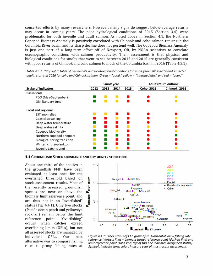
About one third of the species in the groundfish FMP have been evaluated at least once for the overfished threshold based on stock assessment results. Most of the recently assessed groundfish species are near or above the biomass limit reference point, and are thus not in an “overfished” status (Fig. 4.4.1). Only two stocks (Pacific ocean perch and yelloweye rockfish) remain below the limit reference point. “Overfishing” occurs when catches exceed overfishing limits (OFLs), but not all assessed stocks are managed by individual OFLs. Our best alternative was to compare fishing rates to proxy fishing rates at

Figure 4.4.1: Stock status of CCE groundfish. Horizontal line = fishing rate reference. Vertical lines = biomass target reference point (dashed line) and limit reference point (solid line; left of this line indicates overfished status). Symbols indicate taxa; colors indicate year of most recent assessment.

14

maximum sustainable yield (FMSY), which are used to set OFL values. The y-axis of Figure 4.4.1 is therefore not a direct measure of overfishing, but rather a measure of whether fishing rates are above proxy rates (F30% for flatfishes, F50% for other groundfish). Only two stocks (black rockfish in California and Washington, both assessed in 2015) are currently being fished above FMSY.

As noted in Section 4.2, YOY rockfish were highly abundant in the Central CCE in 2015. It will be several years before these fish are large enough to be caught in bottom trawls; thus we will have to wait to determine if the anomalous climate of 2014-2015 affects groundfish populations.

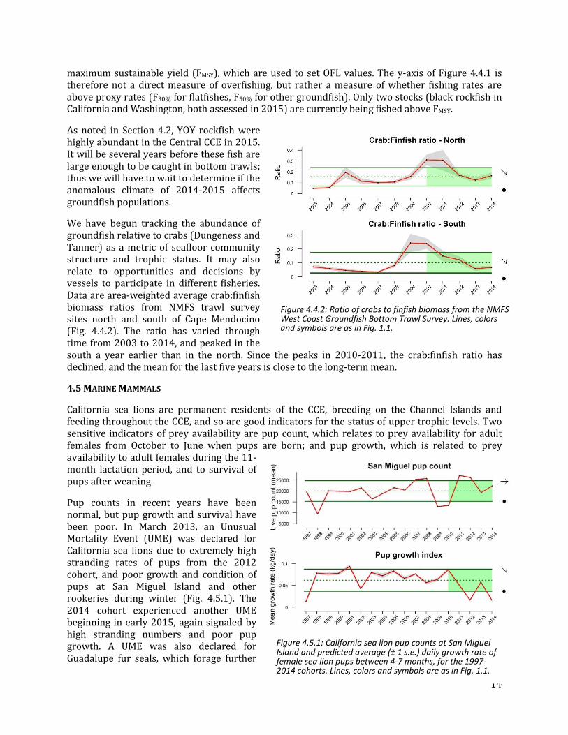
We have begun tracking the abundance of groundfish relative to crabs (Dungeness and Tanner) as a metric of seafloor community structure and trophic status. It may also relate to opportunities and decisions by vessels to participate in different fisheries. Data are area-weighted average crab:finfish biomass ratios from NMFS trawl survey sites north and south of Cape Mendocino (Fig. 4.4.2). The ratio has varied through time from 2003 to 2014, and peaked in the south a year earlier than in the north. Since the peaks in 2010-2011, the crab:finfish ratio has declined, and the mean for the last five years is close to the long-term mean.

4.5 MARINE MAMMALS

California sea lions are permanent residents of the CCE, breeding on the Channel Islands and feeding throughout the CCE, and so are good indicators for the status of upper trophic levels. Two sensitive indicators of prey availability are pup count, which relates to prey availability for adult females from October to June when pups are born; and pup growth, which is related to prey availability to adult females during the 11-month lactation period, and to survival of pups after weaning.

Pup counts in recent years have been normal, but pup growth and survival have been poor. In March 2013, an Unusual Mortality Event (UME) was declared for California sea lions due to extremely high stranding rates of pups from the 2012 cohort, and poor growth and condition of pups at San Miguel Island and other rookeries during winter (Fig. 4.5.1). The 2014 cohort experienced another UME beginning in early 2015, again signaled by high stranding numbers and poor pup growth. A UME was also declared for Guadalupe fur seals, which forage further

Figure 4.5.1: California sea lion pup counts at San Miguel Island and predicted average (± 1 s.e.) daily growth rate of female sea lion pups between 4-7 months, for the 1997-2014 cohorts. Lines, colors and symbols are as in Fig. 1.1.

Figure 4.4.2: Ratio of crabs to finfish biomass from the NMFS West Coast Groundfish Bottom Trawl Survey. Lines, colors and symbols are as in Fig. 1.1.

15

offshore. The decline in pup production of these species reflects the large spatial extent of poor foraging conditions for pinnipeds in the southern CCE.

4.6 SEABIRDS

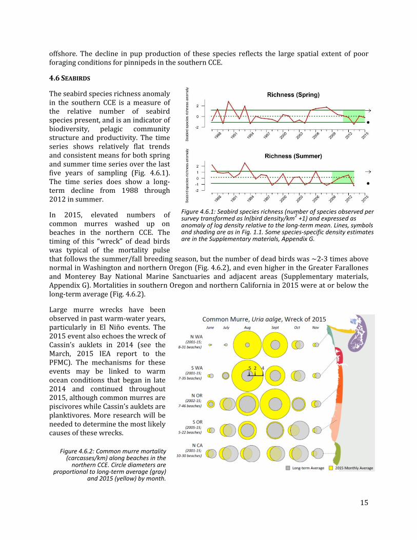
The seabird species richness anomaly in the southern CCE is a measure of the relative number of seabird species present, and is an indicator of biodiversity, pelagic community structure and productivity. The time series shows relatively flat trends and consistent means for both spring and summer time series over the last five years of sampling (Fig. 4.6.1). The time series does show a long-term decline from 1988 through 2012 in summer.

In 2015, elevated numbers of common murres washed up on beaches in the northern CCE. The timing of this “wreck” of dead birds was typical of the mortality pulse that follows the summer/fall breeding season, but the number of dead birds was ~2-3 times above normal in Washington and northern Oregon (Fig. 4.6.2), and even higher in the Greater Farallones and Monterey Bay National Marine Sanctuaries and adjacent areas (Supplementary materials, Appendix G). Mortalities in southern Oregon and northern California in 2015 were at or below the long-term average (Fig. 4.6.2).

Large murre wrecks have been observed in past warm-water years, particularly in El Niño events. The 2015 event also echoes the wreck of Cassin’s auklets in 2014 (see the March, 2015 IEA report to the PFMC). The mechanisms for these events may be linked to warm ocean conditions that began in late 2014 and continued throughout 2015, although common murres are piscivores while Cassin’s auklets are planktivores. More research will be needed to determine the most likely causes of these wrecks.

Figure 4.6.1: Seabird species richness (number of species observed per survey transformed as ln(bird density/km

2 +1) and expressed as

anomaly of log density relative to the long-term mean. Lines, symbols and shading are as in Fig. 1.1. Some species-specific density estimates are in the Supplementary materials, Appendix G.

Figure 4.6.2: Common murre mortality (carcasses/km) along beaches in the

northern CCE. Circle diameters are proportional to long-term average (gray)

and 2015 (yellow) by month.

16

5 HUMAN ACTIVITIES

5.1 TOTAL LANDINGS BY MAJOR FISHERIES

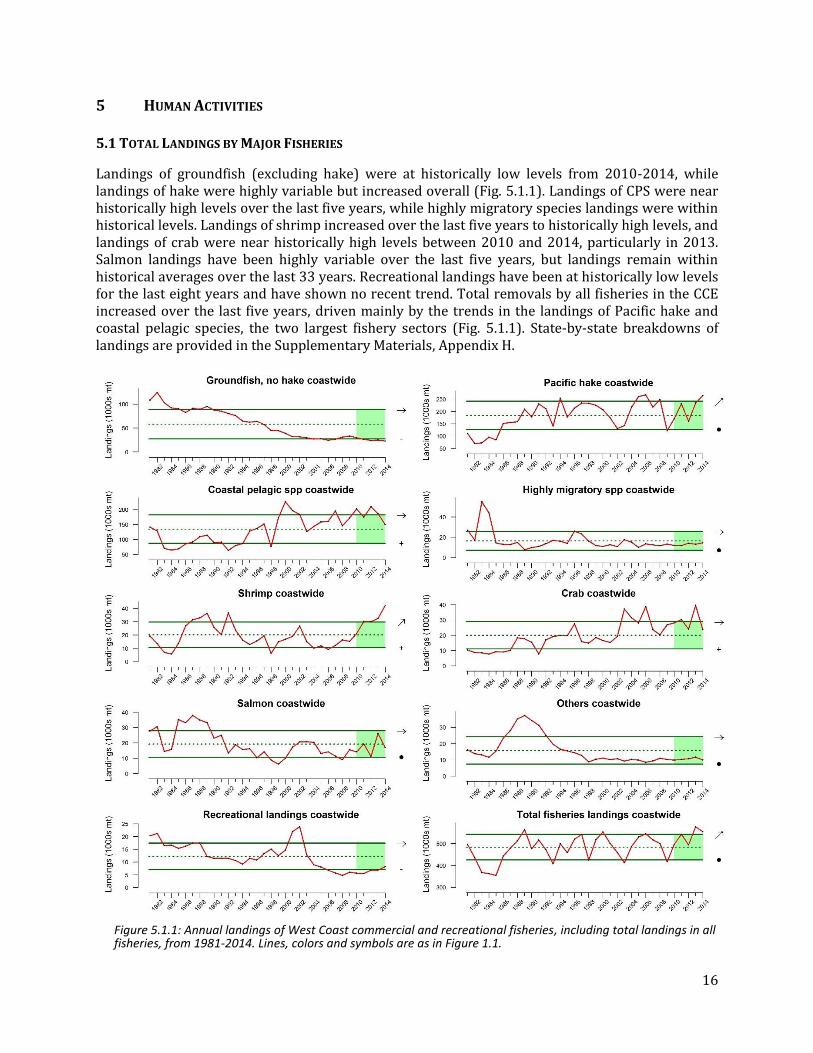
Landings of groundfish (excluding hake) were at historically low levels from 2010-2014, while landings of hake were highly variable but increased overall (Fig. 5.1.1). Landings of CPS were near historically high levels over the last five years, while highly migratory species landings were within historical levels. Landings of shrimp increased over the last five years to historically high levels, and landings of crab were near historically high levels between 2010 and 2014, particularly in 2013. Salmon landings have been highly variable over the last five years, but landings remain within historical averages over the last 33 years. Recreational landings have been at historically low levels for the last eight years and have shown no recent trend. Total removals by all fisheries in the CCE increased over the last five years, driven mainly by the trends in the landings of Pacific hake and coastal pelagic species, the two largest fishery sectors (Fig. 5.1.1). State-by-state breakdowns of landings are provided in the Supplementary Materials, Appendix H.

Figure 5.1.1: Annual landings of West Coast commercial and recreational fisheries, including total landings in all fisheries, from 1981-2014. Lines, colors and symbols are as in Figure 1.1.

17

5.2 SEAFLOOR DISTURBANCE BY FISHING GEAR

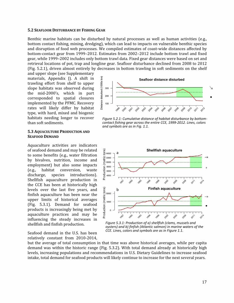
Benthic marine habitats can be disturbed by natural processes as well as human activities (e.g., bottom contact fishing, mining, dredging), which can lead to impacts on vulnerable benthic species and disruption of food web processes. We compiled estimates of coast-wide distances affected by bottom-contact gear from 1999–2012. Estimates from 2002–2012 include bottom trawl and fixed gear, while 1999–2002 includes only bottom trawl data. Fixed gear distances were based on set and retrieval locations of pot, trap and longline gear. Seafloor disturbance declined from 2008 to 2012 (Fig. 5.2.1), driven almost entirely by decreases in bottom trawling in soft sediments on the shelf and upper slope (see Supplementary materials, Appendix J). A shift in trawling effort from shelf to upper slope habitats was observed during the mid-2000’s, which in part corresponded to spatial closures implemented by the PFMC. Recovery rates will likely differ by habitat type, with hard, mixed and biogenic habitats needing longer to recover than soft sediments.

5.3 AQUACULTURE PRODUCTION AND

SEAFOOD DEMAND

Aquaculture activities are indicators of seafood demand and may be related to some benefits (e.g., water filtration by bivalves, nutrition, income and employment) but also some impacts (e.g., habitat conversion, waste discharge, species introductions). Shellfish aquaculture production in the CCE has been at historically high levels over the last five years, and finfish aquaculture has been near the upper limits of historical averages (Fig. 5.3.1). Demand for seafood products is increasingly being met by aquaculture practices and may be influencing the steady increases in shellfish and finfish production.

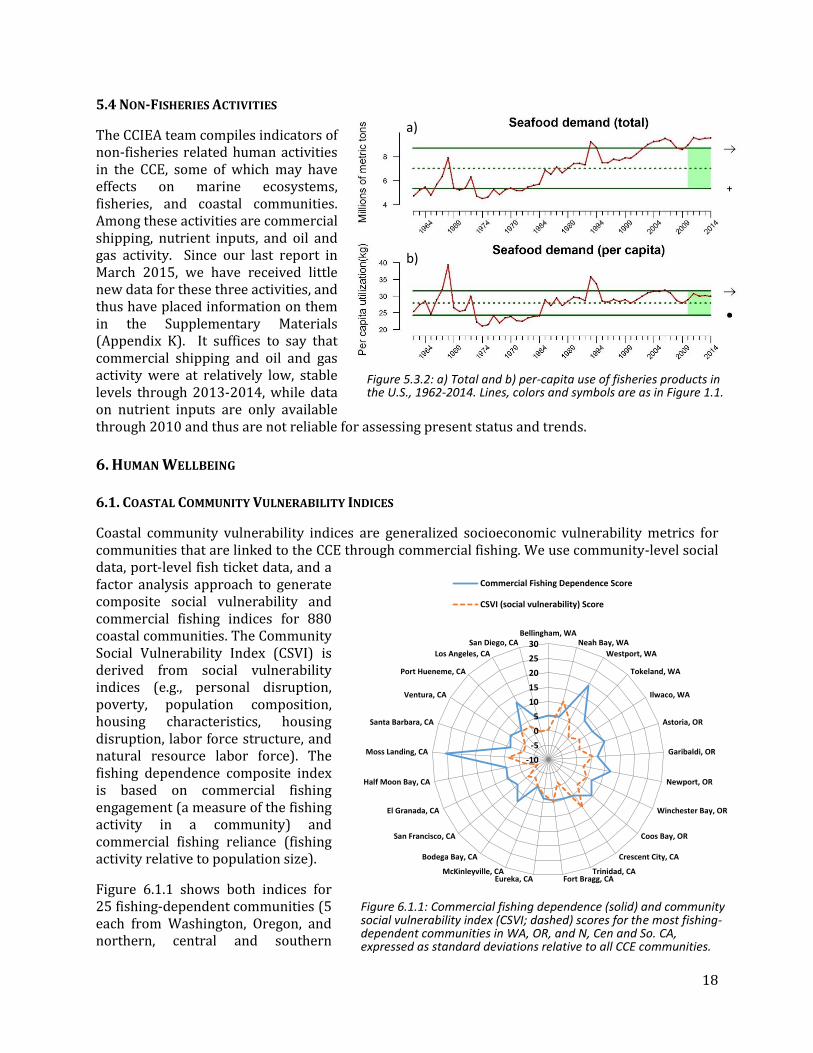
Seafood demand in the U.S. has been relatively constant from 2010-2014, but the average of total consumption in that time was above historical averages, while per capita demand was within the historic range (Fig. 5.3.2). With total demand already at historically high levels, increasing populations and recommendations in U.S. Dietary Guidelines to increase seafood intake, total demand for seafood products will likely continue to increase for the next several years.

Figure 5.2.1: Cumulative distance of habitat disturbance by bottom-contact fishing gear across the entire CCE, 1999-2012. Lines, colors and symbols are as in Fig. 1.1.

Seafloor distance disturbed

a

)

b

)

Figure 5.3.1: Production of a) shellfish (clams, mussels and oysters) and b) finfish (Atlantic salmon) in marine waters of the CCE. Lines, colors and symbols are as in Figure 1.1.

18

5.4 NON-FISHERIES ACTIVITIES

The CCIEA team compiles indicators of non-fisheries related human activities in the CCE, some of which may have effects on marine ecosystems, fisheries, and coastal communities. Among these activities are commercial shipping, nutrient inputs, and oil and gas activity. Since our last report in March 2015, we have received little new data for these three activities, and thus have placed information on them in the Supplementary Materials (Appendix K). It suffices to say that commercial shipping and oil and gas activity were at relatively low, stable levels through 2013-2014, while data on nutrient inputs are only available through 2010 and thus are not reliable for assessing present status and trends.

6. HUMAN WELLBEING

6.1. COASTAL COMMUNITY VULNERABILITY INDICES

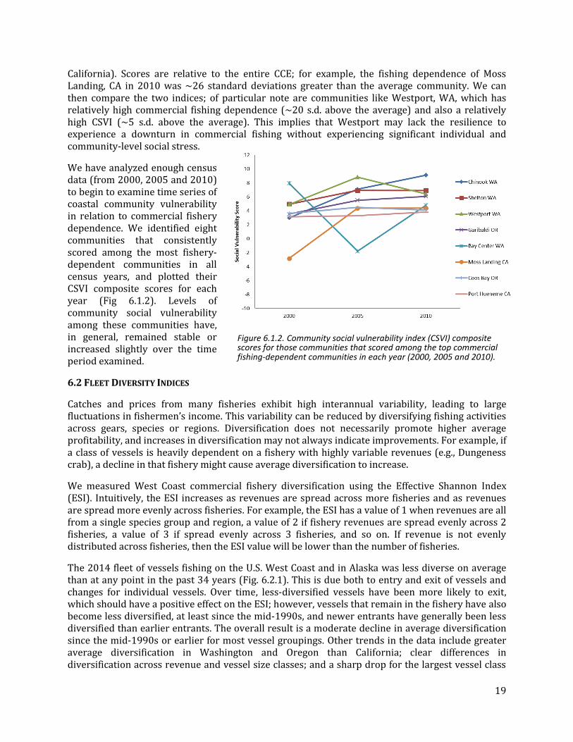
Coastal community vulnerability indices are generalized socioeconomic vulnerability metrics for communities that are linked to the CCE through commercial fishing. We use community-level social data, port-level fish ticket data, and a factor analysis approach to generate composite social vulnerability and commercial fishing indices for 880 coastal communities. The Community Social Vulnerability Index (CSVI) is derived from social vulnerability indices (e.g., personal disruption, poverty, population composition, housing characteristics, housing disruption, labor force structure, and natural resource labor force). The fishing dependence composite index is based on commercial fishing engagement (a measure of the fishing activity in a community) and commercial fishing reliance (fishing activity relative to population size).

Figure 6.1.1 shows both indices for 25 fishing-dependent communities (5 each from Washington, Oregon, and northern, central and southern

Figure 5.3.2: a) Total and b) per-capita use of fisheries products in the U.S., 1962-2014. Lines, colors and symbols are as in Figure 1.1.

a)

b)

-10

-5

0

5

10

15

20

25

30Bellingham, WA

Neah Bay, WA

Westport, WA

Tokeland, WA

Ilwaco, WA

Astoria, OR

Garibaldi, OR

Newport, OR

Winchester Bay, OR

Coos Bay, OR

Crescent City, CA

Trinidad, CAFort Bragg, CAEureka, CA

McKinleyville, CA

Bodega Bay, CA

San Francisco, CA

El Granada, CA

Half Moon Bay, CA

Moss Landing, CA

Santa Barbara, CA

Ventura, CA

Port Hueneme, CA

Los Angeles, CA

San Diego, CA

Commercial Fishing Dependence Score

CSVI (social vulnerability) Score

Figure 6.1.1: Commercial fishing dependence (solid) and community social vulnerability index (CSVI; dashed) scores for the most fishing-dependent communities in WA, OR, and N, Cen and So. CA, expressed as standard deviations relative to all CCE communities.

19

California). Scores are relative to the entire CCE; for example, the fishing dependence of Moss Landing, CA in 2010 was ~26 standard deviations greater than the average community. We can then compare the two indices; of particular note are communities like Westport, WA, which has relatively high commercial fishing dependence (~20 s.d. above the average) and also a relatively high CSVI (~5 s.d. above the average). This implies that Westport may lack the resilience to experience a downturn in commercial fishing without experiencing significant individual and community-level social stress.

We have analyzed enough census data (from 2000, 2005 and 2010) to begin to examine time series of coastal community vulnerability in relation to commercial fishery dependence. We identified eight communities that consistently scored among the most fishery-dependent communities in all census years, and plotted their CSVI composite scores for each year (Fig 6.1.2). Levels of community social vulnerability among these communities have, in general, remained stable or increased slightly over the time period examined.

6.2 FLEET DIVERSITY INDICES

Catches and prices from many fisheries exhibit high interannual variability, leading to large fluctuations in fishermen’s income. This variability can be reduced by diversifying fishing activities across gears, species or regions. Diversification does not necessarily promote higher average profitability, and increases in diversification may not always indicate improvements. For example, if a class of vessels is heavily dependent on a fishery with highly variable revenues (e.g., Dungeness crab), a decline in that fishery might cause average diversification to increase.

We measured West Coast commercial fishery diversification using the Effective Shannon Index (ESI). Intuitively, the ESI increases as revenues are spread across more fisheries and as revenues are spread more evenly across fisheries. For example, the ESI has a value of 1 when revenues are all from a single species group and region, a value of 2 if fishery revenues are spread evenly across 2 fisheries, a value of 3 if spread evenly across 3 fisheries, and so on. If revenue is not evenly distributed across fisheries, then the ESI value will be lower than the number of fisheries.

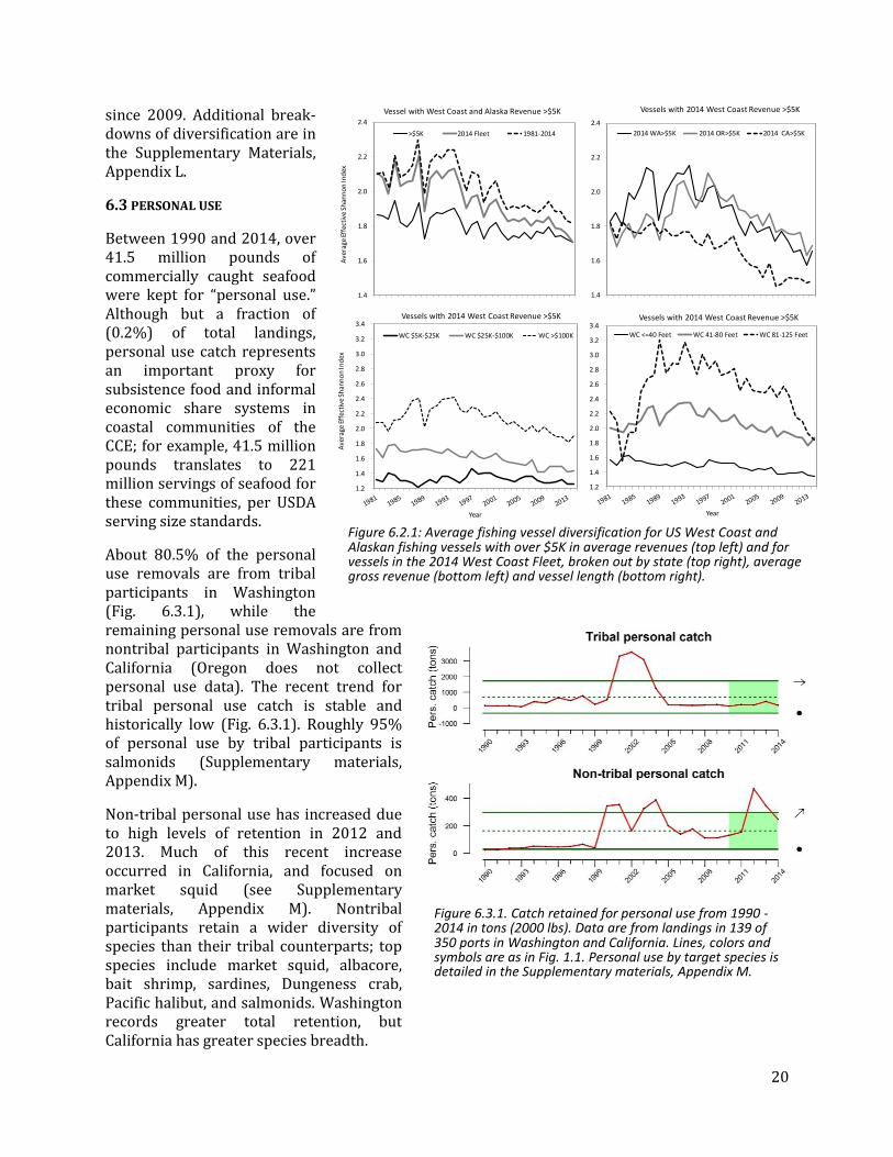
The 2014 fleet of vessels fishing on the U.S. West Coast and in Alaska was less diverse on average than at any point in the past 34 years (Fig. 6.2.1). This is due both to entry and exit of vessels and changes for individual vessels. Over time, less-diversified vessels have been more likely to exit, which should have a positive effect on the ESI; however, vessels that remain in the fishery have also become less diversified, at least since the mid-1990s, and newer entrants have generally been less diversified than earlier entrants. The overall result is a moderate decline in average diversification since the mid-1990s or earlier for most vessel groupings. Other trends in the data include greater average diversification in Washington and Oregon than California; clear differences in diversification across revenue and vessel size classes; and a sharp drop for the largest vessel class

Figure 6.1.2. Community social vulnerability index (CSVI) composite scores for those communities that scored among the top commercial fishing-dependent communities in each year (2000, 2005 and 2010).

20

since 2009. Additional break-downs of diversification are in the Supplementary Materials, Appendix L.

6.3 PERSONAL USE

Between 1990 and 2014, over 41.5 million pounds of commercially caught seafood were kept for “personal use.” Although but a fraction of (0.2%) of total landings, personal use catch represents an important proxy for subsistence food and informal economic share systems in coastal communities of the CCE; for example, 41.5 million pounds translates to 221 million servings of seafood for these communities, per USDA serving size standards.

About 80.5% of the personal use removals are from tribal participants in Washington (Fig. 6.3.1), while the remaining personal use removals are from nontribal participants in Washington and California (Oregon does not collect personal use data). The recent trend for tribal personal use catch is stable and historically low (Fig. 6.3.1). Roughly 95% of personal use by tribal participants is salmonids (Supplementary materials, Appendix M).

Non-tribal personal use has increased due to high levels of retention in 2012 and 2013. Much of this recent increase occurred in California, and focused on market squid (see Supplementary materials, Appendix M). Nontribal participants retain a wider diversity of species than their tribal counterparts; top species include market squid, albacore, bait shrimp, sardines, Dungeness crab, Pacific halibut, and salmonids. Washington records greater total retention, but California has greater species breadth.

Figure 6.3.1. Catch retained for personal use from 1990 - 2014 in tons (2000 lbs). Data are from landings in 139 of 350 ports in Washington and California. Lines, colors and symbols are as in Fig. 1.1. Personal use by target species is detailed in the Supplementary materials, Appendix M.

1.4

1.6

1.8

2.0

2.2

2.4

Ave

rage

Eff

ecti

ve S

han

no

n In

dex

Vessel with West Coast and Alaska Revenue >$5K

>$5K 2014 Fleet 1981-2014

1.4

1.6

1.8

2.0

2.2

2.4

Vessels with 2014 West Coast Revenue >$5K

2014 WA>$5K 2014 OR>$5K 2014 CA>$5K

1.2

1.4

1.6

1.8

2.0

2.2

2.4

2.6

2.8

3.0

3.2

3.4

Year

Vessels with 2014 West Coast Revenue >$5K

WC <=40 Feet WC 41-80 Feet WC 81-125 Feet

1.2

1.4

1.6

1.8

2.0

2.2

2.4

2.6

2.8

3.0

3.2

3.4

Ave

rage

Eff

ecti

ve S

han

no

n In

dex

Year

Vessels with 2014 West Coast Revenue >$5K

WC $5K-$25K WC $25K-$100K WC >$100K

Figure 6.2.1: Average fishing vessel diversification for US West Coast and Alaskan fishing vessels with over $5K in average revenues (top left) and for vessels in the 2014 West Coast Fleet, broken out by state (top right), average gross revenue (bottom left) and vessel length (bottom right).