1. Introduction

Most panel data suffer from attrition

In practical work, not much is done to deal with this problem (MCARassumption).

If attrition is taken into account, usually MAR (Selection onobservables) is assumed.

The reason is that it is much more difficult (read: impossible) tocorrect for Non-ignorable attrition (selection on unobservables).

If refreshment samples are available, something can be done.

The Stata-command attrition_model aims to make correcting fornon-ignorable attrition easier.

Its implementation shows the usefulness of structures and pointersin Mata.

·

·

·

·

·

·

·

/

/

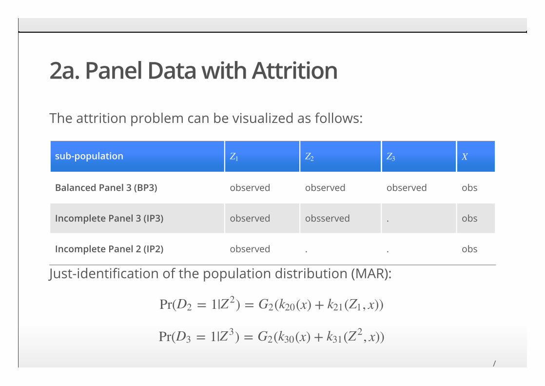
2a. Panel Data with Attrition

The attrition problem can be visualized as follows:

sub-population

Balanced Panel 3 (BP3) observed observed observed obs

Incomplete Panel 3 (IP3) observed obsserved . obs

Incomplete Panel 2 (IP2) observed . . obs

Just-identification of the population distribution (MAR):

Z1 Z2 Z3 X

Pr( = 1| ) = ( (x) + ( , x))D2 Z2 G2 k20 k21 Z1

Pr( = 1| ) = ( (x) + ( , x))D3 Z3 G2 k30 k31 Z2

/

/

2b. The Problem With Non-ignorableAttrition

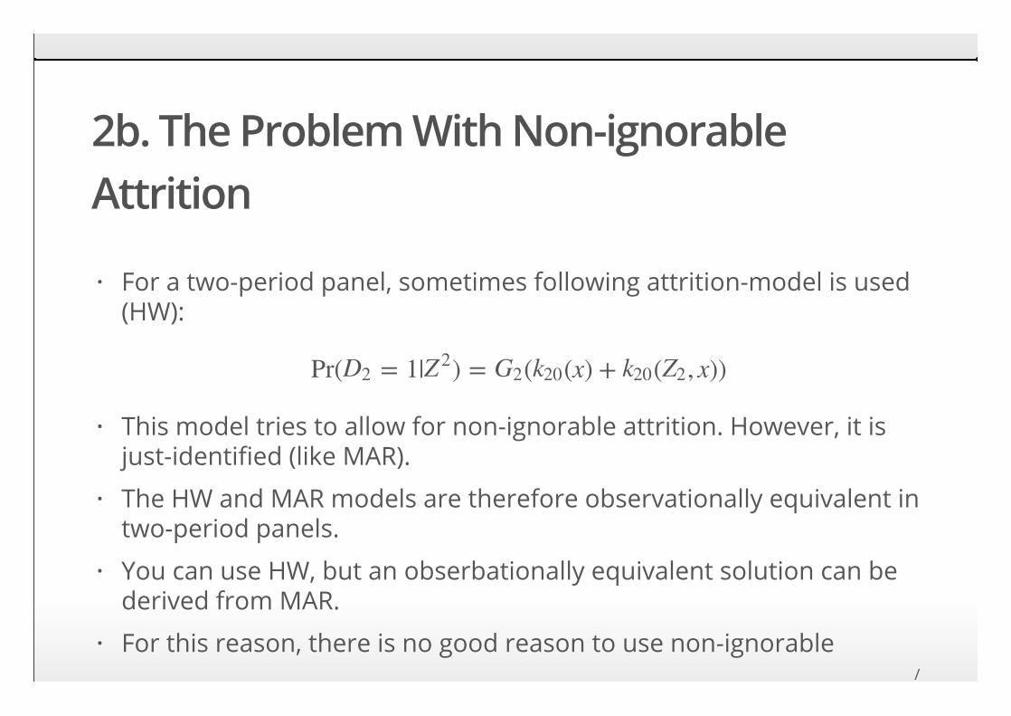
For a two-period panel, sometimes following attrition-model is used(HW):

This model tries to allow for non-ignorable attrition. However, it isjust-identified (like MAR).

The HW and MAR models are therefore observationally equivalent intwo-period panels.

You can use HW, but an obserbationally equivalent solution can bederived from MAR.

For this reason, there is no good reason to use non-ignorable

attrition models.

·

Pr( = 1| ) = ( (x) + ( , x))D2 Z2 G2 k20 k20 Z2

·

·

·

·/

attrition models./

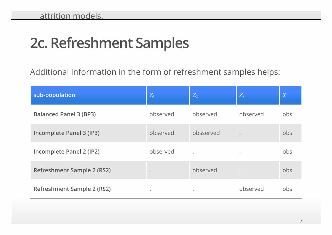
2c. Refreshment Samples

Additional information in the form of refreshment samples helps:

sub-population

Balanced Panel 3 (BP3) observed observed observed obs

Incomplete Panel 3 (IP3) observed obsserved . obs

Incomplete Panel 2 (IP2) observed . . obs

Refreshment Sample 2 (RS2) . observed . obs

Refreshment Sample 2 (RS2) . . observed obs

Z1 Z2 Z3 X

/

/

2d. Identification With RefreshmentSamples (SAN)

Hoonhout and Ridder (2016) show that the SAN model just-identifiesthe population distribution:

SAN stands for Sequential Additively Non-ignorable.

This generalizes the two-period panel result of Hirano, Imbens,Ridder and Rubin (Econometrica, 2001).

·

Pr( = 1| ) = ( (x) + ( , x) + ( , x))D2 Z2 G2 k20 k21 Z1 k20 Z2

Pr( = 1| ) = ( (x) + ( , x) + ( , x))D3 Z3 G2 k30 k31 Z2 k32 Z3

·

·

/

/

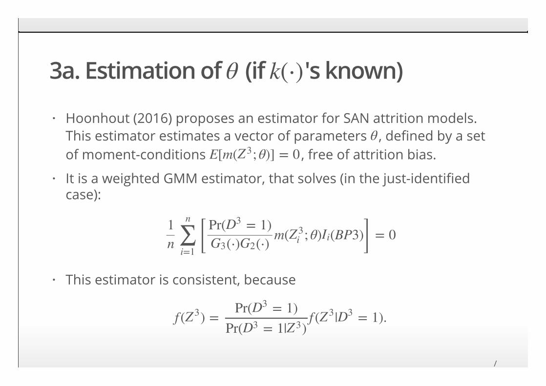
3a. Estimation of (if 's known)θ k(Þ)

Hoonhout (2016) proposes an estimator for SAN attrition models.This estimator estimates a vector of parameters , defined by a setof moment-conditions , free of attrition bias.

It is a weighted GMM estimator, that solves (in the just-identifiedcase):

This estimator is consistent, because

·θ

E[m( ; θ)] = 0Z3

·

[ m( ; θ) (BP3)] = 01n ∑

i=1

n Pr( = 1)D3

(Þ) (Þ)G3 G2Z3

i Ii

·

f ( ) = f ( | = 1).Z3 Pr( = 1)D3

Pr( = 1| )D3 Z3Z3 D3

/

/

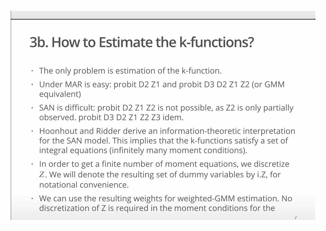
3b. How to Estimate the k-functions?

The only problem is estimation of the k-function.

Under MAR is easy: probit D2 Z1 and probit D3 D2 Z1 Z2 (or GMMequivalent)

SAN is difficult: probit D2 Z1 Z2 is not possible, as Z2 is only partiallyobserved. probit D3 D2 Z1 Z2 Z3 idem.

Hoonhout and Ridder derive an information-theoretic interpretationfor the SAN model. This implies that the k-functions satisfy a set ofintegral equations (infinitely many moment conditions).

In order to get a finite number of moment equations, we discretize . We will denote the resulting set of dummy variables by i.Z, for

notational convenience.

We can use the resulting weights for weighted-GMM estimation. Nodiscretization of Z is required in the moment conditions for the

population model!

·

·

·

·

·Z

·

/

population model!/

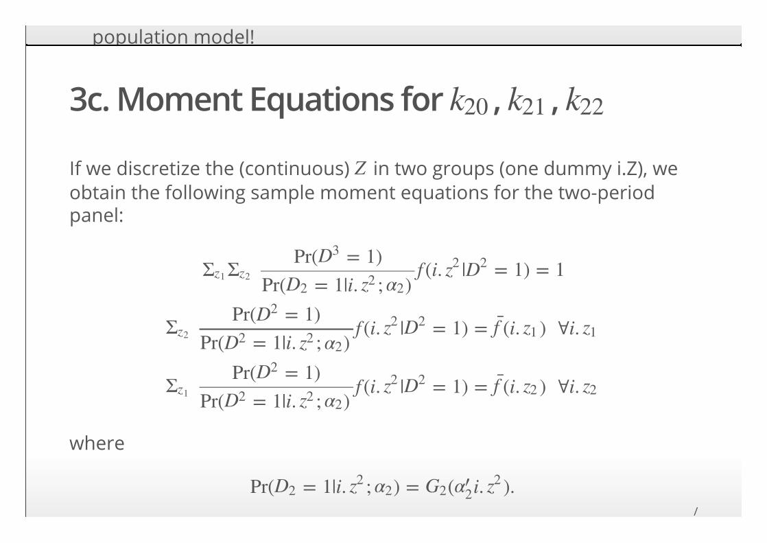
3c. Moment Equations for , ,

If we discretize the (continuous) in two groups (one dummy i.Z), weobtain the following sample moment equations for the two-periodpanel:

where

This requires a lot of book-keeping…

k20 k21 k22

Z

f (i. | = 1) = 1Σz1Σz2

Pr( = 1)D3

Pr( = 1|i. ; )D2 z2 α2z2 D2

f (i. | = 1) = (i. ) �i.Σz2

Pr( = 1)D2

Pr( = 1|i. ; )D2 z2 α2z2 D2 f̄ z1 z1

f (i. | = 1) = (i. ) �i.Σz1

Pr( = 1)D2

Pr( = 1|i. ; )D2 z2 α2z2 D2 f̄ z2 z2

Pr( = 1|i. ; ) = ( i. ).D2 z2 α2 G2 α′2 z2

/

This requires a lot of book-keeping…/

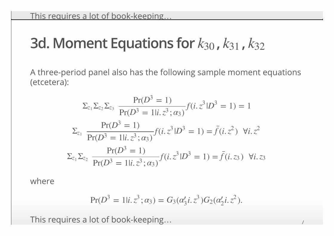
3d. Moment Equations for , ,

A three-period panel also has the following sample moment equations(etcetera):

where

This requires a lot of book-keeping…

k30 k31 k32

f (i. | = 1) = 1Σz1Σz2Σz3

Pr( = 1)D3

Pr( = 1|i. ; )D3 z3 α3z3 D3

f (i. | = 1) = (i. ) �i.Σz1

Pr( = 1)D3

Pr( = 1|i. ; )D3 z3 α3z3 D3 f̄ z2 z2

f (i. | = 1) = (i. ) �i.Σz1Σz2

Pr( = 1)D3

Pr( = 1|i. ; )D3 z3 α3z3 D3 f̄ z3 z3

Pr( = 1|i. ; ) = ( i. ) ( i. ).D3 z3 α3 G3 α′3 z3 G2 α′

2 z2

/

This requires a lot of book-keeping… /

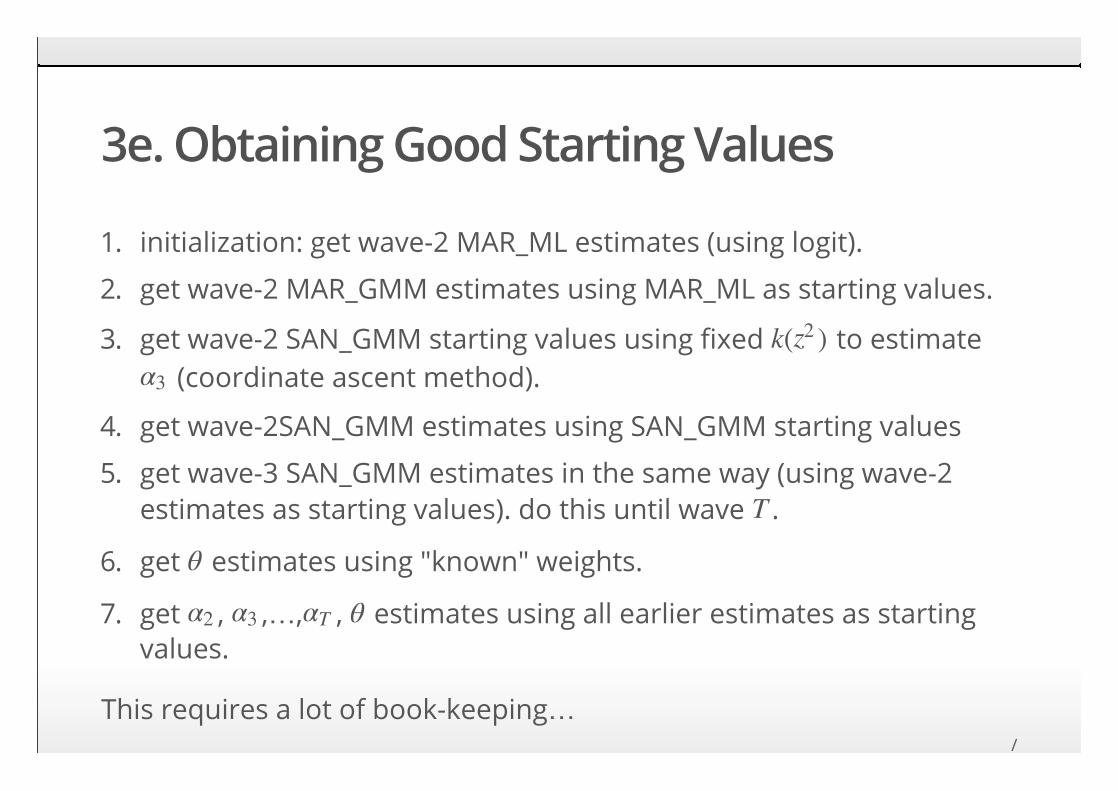
3e. Obtaining Good Starting Values

This requires a lot of book-keeping…

1. initialization: get wave-2 MAR_ML estimates (using logit).

2. get wave-2 MAR_GMM estimates using MAR_ML as starting values.

3. get wave-2 SAN_GMM starting values using fixed to estimate (coordinate ascent method).

4. get wave-2SAN_GMM estimates using SAN_GMM starting values

5. get wave-3 SAN_GMM estimates in the same way (using wave-2estimates as starting values). do this until wave .

6. get estimates using "known" weights.

7. get , ,…, , estimates using all earlier estimates as startingvalues.

k( )z2

α3

T

θ

α2 α3 αT θ

/

/

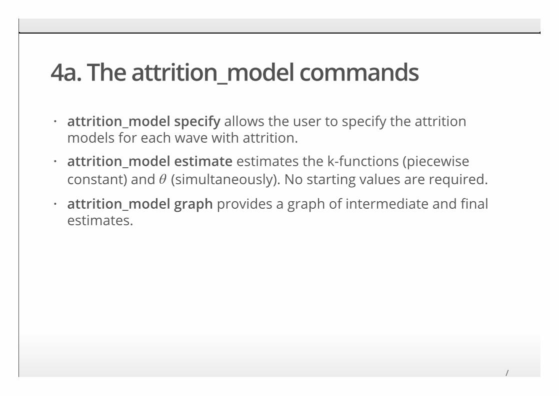
4a. The attrition_model commands

attrition_model specify allows the user to specify the attritionmodels for each wave with attrition.

attrition_model estimate estimates the k-functions (piecewiseconstant) and (simultaneously). No starting values are required.

attrition_model graph provides a graph of intermediate and finalestimates.

·

·θ

·

/

/

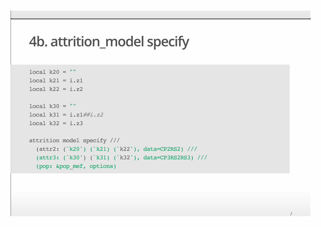
4b. attrition_model specify

local k20 = ""local k21 = i.z1local k22 = i.z2

local k30 = ""local k31 = i.z1##i.z2local k32 = i.z3

attrition model specify /// (attr2: (̀k20') (̀k21) (̀k22'), data=CP2RS2) /// (attr3: (̀k30') (̀k31) (̀k32'), data=CP3RS2RS3) /// (pop: &pop_mef, options)

/

/

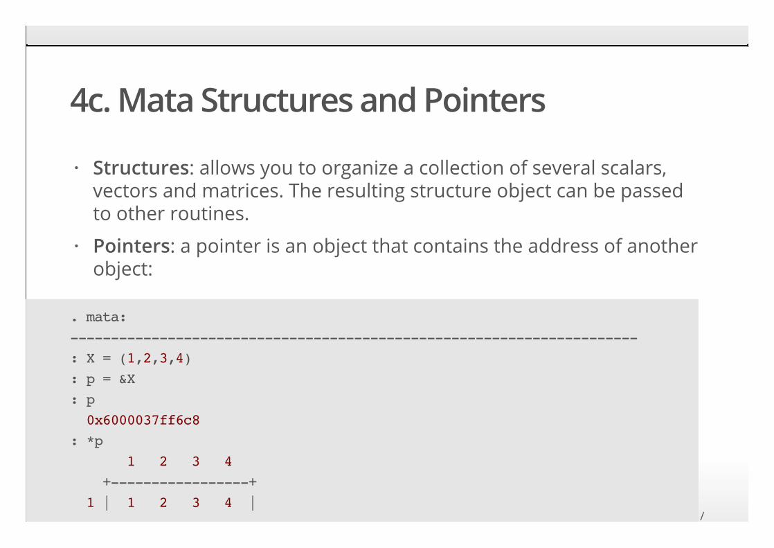
4c. Mata Structures and Pointers

Structures: allows you to organize a collection of several scalars,vectors and matrices. The resulting structure object can be passedto other routines.

Pointers: a pointer is an object that contains the address of anotherobject:

·

·

. mata:----------------------------------------------------------------------: X = (1,2,3,4): p = &X: p 0x6000037ff6c8: *p 1 2 3 4 +-----------------+ 1 | 1 2 3 4 |

/

+-----------------+/

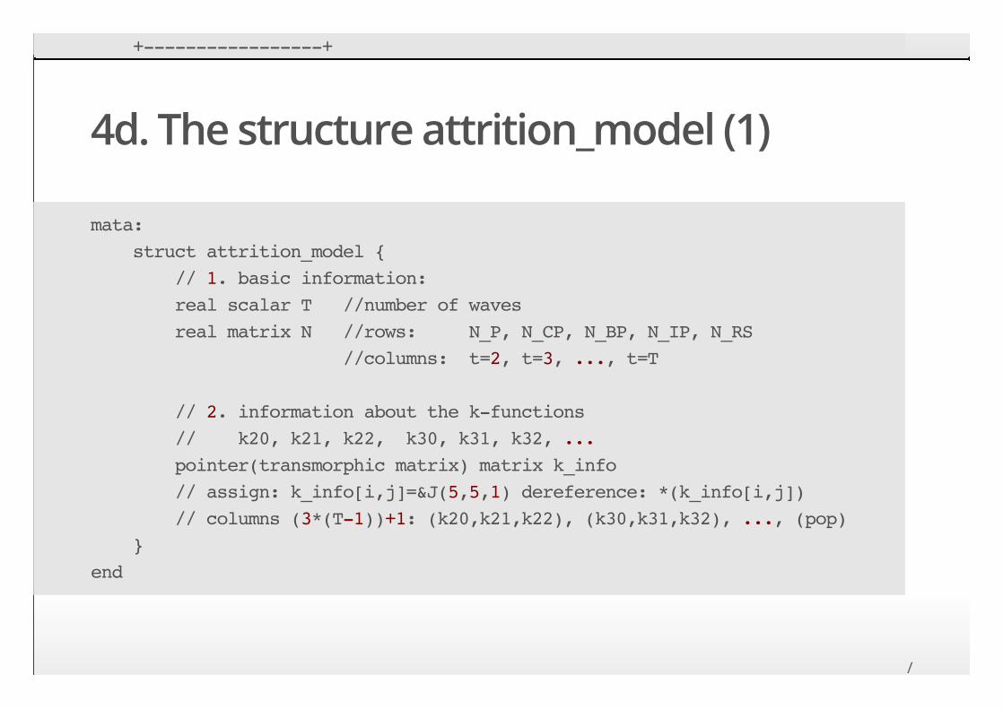
4d. The structure attrition_model (1)

mata: struct attrition_model { // 1. basic information: real scalar T //number of waves real matrix N //rows: N_P, N_CP, N_BP, N_IP, N_RS //columns: t=2, t=3, ..., t=T // 2. information about the k-functions // k20, k21, k22, k30, k31, k32, ... pointer(transmorphic matrix) matrix k_info // assign: k_info[i,j]=&J(5,5,1) dereference: *(k_info[i,j]) // columns (3*(T-1))+1: (k20,k21,k22), (k30,k31,k32), ..., (pop) }end

/

/

4e. The structure attrition_model (2)

The structure includes a variable that is of type "matrix of pointers."

Each column of this matrix describes a k-function. That is, if the columns are , , , , , .

Each row describes particular information for each k-function.

This structure facilitates the book-keeping enormously.

·

· T = 3k20 k21 k22 k30 k31 k32

·

For instance, the first row contains the parameter-names of .

The second row stores the estimated values (for use in theestimation in later waves).

Another row contains the MAR estimates of the k-functionparameters (estimated at the time of initialization of thestructure, within attrition_specify).

-, . . . ,α20 α32

-

-

·/

/

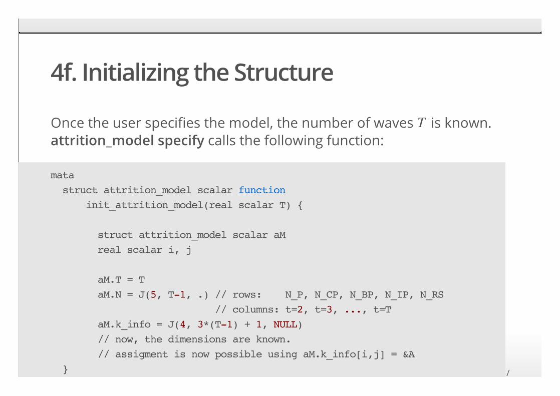
4f. Initializing the Structure

Once the user specifies the model, the number of waves is known.attrition_model specify calls the following function:

T

mata struct attrition_model scalar function init_attrition_model(real scalar T) { struct attrition_model scalar aM real scalar i, j aM.T = T aM.N = J(5, T-1, .) // rows: N_P, N_CP, N_BP, N_IP, N_RS // columns: t=2, t=3, ..., t=T aM.k_info = J(4, 3*(T-1) + 1, NULL) // now, the dimensions are known. // assigment is now possible using aM.k_info[i,j] = &A } /

end/

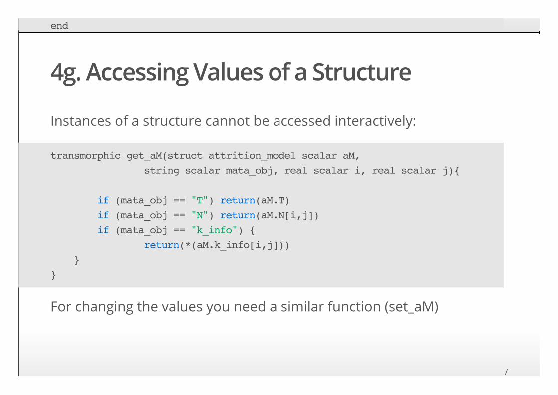
4g. Accessing Values of a Structure

Instances of a structure cannot be accessed interactively:

For changing the values you need a similar function (set_aM)

transmorphic get_aM(struct attrition_model scalar aM, string scalar mata_obj, real scalar i, real scalar j){

if (mata_obj == "T") return(aM.T) if (mata_obj == "N") return(aM.N[i,j]) if (mata_obj == "k_info") { return(*(aM.k_info[i,j])) }}

/

/

4h. attrition_model estimate

Many estimations are done here, before arriving at the finalestimates.

All the estimations are similar but different.

The idea is to write a single moment-evaluator-function. Thismoment-evaluator function morphs automatically into the moment-evaluator-function that is required for the current estimation.

This can be achieved because the gmm-command allows us to passextra arguments to the moment-evaluator function. We will simplypass the structure aM (of type attrition_model) to the evaluatorfunction. With this information it can morph as required.

·

·

·

·

/

/

5. Conclusion

The attrition_model command provides a relatively straightforwardway to obtain panel-data model estimates that are corrected for(potentially non-ignorable) attrition. The user can specify each of the k-functions separately, to keep the number of nuisance parameterswithin bounds.

1. All the book-keeping in attrition_model estimate is relegated toone or more instances of a structure. This structure is passed to themoment-evaluator function.

2. This structure contains a matrix of pointers. The columns of thatmatrix does the book-keeping for one k-function.

/