Supplementary Material

Development of a Satellite-based Model for Estimating the Long-

term Spatiotemporal Exposure to NO2

Bijan Yeganeh1, 2, Michael G. Hewson3, Samuel Clifford2, 4, Ahmad Tavassoli5, Luke D.

Knibbs6, and Lidia Morawska1

1 International Laboratory for Air Quality and Health, Queensland University of Technology, Brisbane, Queensland 4001, Australia

2 Centre for Air quality and health Research and evaluation, Glebe, New South Wales 2037, Australia

3 School of Education and the Arts, Central Queensland University, North Rockhampton, Queensland 4702, Australia

4 ARC Centre of Excellence for Mathematical and Statistical Frontiers, Queensland University of Technology, Brisbane, Queensland 4001, Australia

5 School of Civil Engineering, The University of Queensland, St Lucia, Queensland 4072, Australia

6 School of Public Health, The University of Queensland, Herston, Queensland 4006, Australia

S1

1. Modelled Planetary Boundary Layer Height and Wind Vectors

The Climate Research Group (CRG) of The University of Queensland (UQ) School of

Geography, Planning and Environment Management provided the planetary boundary layer

(PBL) height and wind vectors (U and V) for the spatial analysis of the project. The Weather

Research and Forecasting model (WRF) was used to calculate daily at 2 pm Australian

Eastern standard Time (AEST): (1) average PBL height in metres above ground level (AGL);

and (2) 10 metre AGL wind vectors. These variables were averaged for each month for six

years (2006 to 2011). The time of 14:00 AEST was chosen to coincide with the instrument

ephemeris calculated Aura satellite overpass time for the study area.

1.1 Weather Model Configuration

WRF is a community “numerical weather prediction and atmospheric simulation system for

both research and operational applications” (Skamarock et al., 2005) that has been evolving

through predecessors for some twenty years. CRG used WRF version 3.5 for this work.

The WRF three dimensional, two domain configuration was designed considering model

guiding documentation (Wang et al., 2012) and a project need to optimise model running

time and still enable at least a moderate model output spatial resolution. The WRF nested

domains were at a 5:1 (outer:inner) ratio as shown in Figure S1. The model domains were

centred at latitude 27.5 degrees south and longitude 152 degrees east – just west of the project

subject city of Brisbane. The outer domain had a spatial resolution of 15 km and the inner

domain was therefore set at 3 km. The domain design, particularly the size of the outer

domain, made optimal use of six-hourly Global Forecasting System (GFS) reanalysed

meteorological data archive. The inner domain size of 3 km was chosen to resolve terrain

features suitable to the GIS based multivariate analysis while not burdening the model run

times unnecessarily. WRF earth surface database best spatial resolution is 30 arc-seconds so

the inner domain spatial resolution matched the geographical initial condition data. While it

S2

has been shown that a WRF 1 km spatial resolution best accounts for topographic effects on

wind flow (Horvath et al., 2012), the project selection of WRF wind vectors (U, V) at 10

metres above ground level combined with the 3 km spatial resoultion provided a suitable

modelled wind surface to use in the GIS enabled multivariate spatial analsysis. The WRF

inner domains was sized to 121 * 121 grid squares – greater than the minimum 100 * 100

grid square size recommended by WRF user guidance (Wang et al., 2012). The model

tropospheric depth was divided into 30 sigma levels.

Figure S1: the WRF model two domain design centred on a location to the west of the Australian city of Brisbane at 27.5 south and 152 degrees east.

GFS 6 hourly, reanalysed meteorology data is provided by the US National Centre for

Environmental Prediction (NCEP) as final operational global tropospheric analysis. Since this

S3

data incorporates weather observations at one degree latitude/longitude a large outer domain

is needed so that sufficient meteorology is provided to the model boundary and initial

conditions. WRF model geographical boundary and initial conditions created by the WRF

Pre-processing System (WPS) were compiled from:

United States Geological Survey (USGS) topography at 30 arc-seconds;

USGS 24 land use categories;

USGS 16 soil categories; and

Standard WRF provided albedo, soil temperature, sea surface temperature and green

fraction data sets.

WRF physics scheme configurations were chosen based on those found optimal for wind

modelling (Deppe et al., 2013; Santos-Alamillos et al., 2013; Yang et al., 2013; Zhang et al.,

2013) and suitable for Australian environmental conditions (Evans et al., 2012). The main

physics scheme selections being:

Microphysics – WSM (WRF single moment) 3-class;

Longwave radiation – RRTM (Rapid Radiative Transfer Model) scheme;

Shortwave scheme – Dudhia scheme;

Surface layer option – Monin-Obukhov scheme;

Land surface option – Unified Noah land-surface model;

Boundary layer option – YSU (Yonsei University) scheme;

Cumulus option (outer domain only) – Kain-Fritsch scheme; and

Vertical velocity damping switched on.

1.2 Weather Model Runs and Data Extraction

WPS and WRF were setup to process one month per model run for the six years; 2006 to

2011. Accordingly, 72 individual WRF model runs were packaged up and run in Australia’s

S4

National Computing Infrastructure. A WRF run time-step of 90 seconds was used. WRF

output was segmented into daily data output files for each month of each year to simplify the

variable extraction process.

WRF netCDF output files were processed with the well-known netCDF Operator (NCO)

software toolkit (Zender, 2008) to extract the three required variables. WRF wind output is

retained as two Cartesian coordinate parameters – U and V wind vector components. “U”

wind is air motion in the “x” direction and “V” wind is air motion in the “y” direction (Stull,

2000). WRF outputs PBL height in a variable PBLH. These three variables were extracted

from the daily files and averaged per month and redeposited in netCDF files retaining the

model grid point latitude and longitude variables so that the files could be ingested into

ArcGIS. The daily files were then used separately to output the maps of each variable for

each day of 2011.

S5

2. Monthly predictions of NO2 concentration in South-east Queensland

The seasons in Australia are described in the following way: Spring - the three transition months September, October and November. Summer - the three hottest months December, January and February. Autumn- the transition months March, April and May (Bureau of Meteorology, 2017).

Figure S2: Monthly average predictions of NO2 concentration in 2006.

S6

Figure S3: Monthly average predictions of NO2 concentration in 2011.

S7

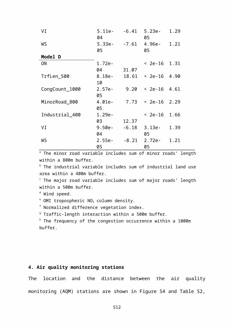
3. Results of input selection

Table S1: Results of input selection for model A, B, C, and D.

Std. Error t value Pr(>|t|) Variance Inflation Factor

Model AMinorRoad_800a 5.77e-05 7.50 2.05e-13 1.82Industrial_400b 1.90e-03 20.40 < 2e-16 1.38MajorRoad_500c 1.01e-04 9.76 < 2e-16 2.01WSd 6.52e-05 -9.44 < 2e-16 1.03Model BONe 1.75e-04 30.64 < 2e-16 1.30MinorRoad_800 3.82e-05 11.32 < 2e-16 1.97Industrial_400 1.24e-03 12.37 < 2e-16 1.46MajorRoad_500 6.49e-05 18.69 < 2e-16 2.05VIf 9.71e-04 -7.36 1.01e-05 1.37WS 4.55e-05 -8.20 2.28e-05 1.23Model CON 2.06e-04 24.25 < 2e-16 1.31TrfLen_500g 1.29e-09 22.07 < 2e-16 4.36CongCount_1000h 6.47e-06 9.20 < 2e-16 4.46Industrial_400 1.59e-03 8.18 < 2e-16 1.65VI 5.11e-04 -6.41 5.23e-05 1.29WS 5.33e-05 -7.61 4.96e-05 1.21Model DON 1.72e-04 31.07 < 2e-16 1.31TrfLen_500 8.18e-10 18.61 < 2e-16 4.90CongCount_1000 2.57e-05 9.20 < 2e-16 4.61MinorRoad_800 4.01e-05 7.73 < 2e-16 2.29Industrial_400 1.29e-03 12.37 < 2e-16 1.66VI 9.50e-04 -6.18 3.13e-05 1.39WS 2.55e-05 -8.21 2.72e-05 1.21

a The minor road variable includes sum of minor roads’ length within a 800m buffer.b The industrial variable includes sum of industrial land use area within a 400m buffer.c The major road variable includes sum of major roads’ length within a 500m buffer.d Wind speed.e OMI tropospheric NO2 column density.f Normalized difference vegetation index.g Traffic-length interaction within a 500m buffer.h The frequency of the congestion occurrence within a 1000m buffer.

S8

4. Air quality monitoring stations

The location and the distance between the air quality monitoring (AQM) stations are shown

in Figure S4 and Table S2, respectively. The spatial resolution of the satellite observations is

13 km × 24 km, while the average distance between the AQM stations in the study area is

52.23 km. Hence, the resolution of the satellite observation is finer than the spatial

distribution of the AQM stations. Therefore, the use of the satellite observations provided

informative data for estimating the NO2 concentration between the stations and improved the

modelling performance.

Figure S4. The location of the air quality monitoring stations in the study area

S9

Six monitoring stations operated during the whole study period, while other stations did not

measure the NO2 concentration continuously throughout the study period. A summary of the

missing data period in the monitoring stations is provided in the following:

Pinkenba: January 2011

Rocklea: March 2008, February 2011 to December 2011

Springwood: February 2006

Toowoomba: January to December 2011

Woolloongabba: January 2006 to March 2008

Wynnum North: January 2006 to August 2007

S10

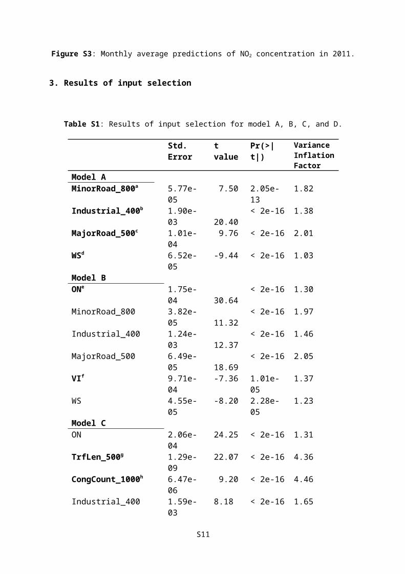
Table S2: The distance between air quality monitoring stations within the study area (km).

Deception

Bay

Flinders

View

Mountain

Creek

Mutdapilly

North Maclea

n

Pinkenba

Rocklea

SouthBrisban

e

Springwood

Toowoomba

Woolloongabba

Wynnum

NorthDeception

Bay 0                      

Flinders View 57.26 0                    

Mountain Creek 56.19 111.88 0                  

Mutdapilly 72.92 16.66 126.32 0                North

Maclean 64.22 28.53 120.35 37.49 0              

Pinkenba 26.62 43.01 81.15 59.26 39.78 0            Rocklea 39.17 25.26 95.33 41.57 25.19 18.43 0          South

Brisbane 32.41 31.68 88.65 48.15 31.79 11.23 7.38 0        

Springwood 47.72 36.1 102.76 50.49 20.52 21.29 15.55 17.53 0      Toowoomba 109.19 75.99 144.78 66.94 103.39 110.89 97.53 101.17 111.28 0    Woolloongab

ba 33.8 31.6 89.37 47.24 30.31 12.19 6.25 1.44 16.43 101.25 0  

Wynnum North 28.99 45.49 82.25 61.76 39.94 3.84 20.18 13.92 20.44 114.37 14.32 0

S11

S12

5. Model evaluation metrics

Different metrics can be used for evaluating the modelling performance. In this study,

the coefficient of determination (R2) was utilized to describe the proportion of the variation in

the dependent variable(s) which can be explained by a model of interest (Yeganeh et al.,

2012), and it is calculated as bellow:

R2=1−∑i =1

n

( Y i−Y i¿ )2

∑i=1

n

(Y i−Y i )2

(1)

In addition, the root mean squared error (RMSE) was used to evaluate the accuracy of

the modelling performance using equation 2:

RMSE=√ 1n∑i=1

n

|Y i−Y i¿|2 (2)

where i indicates the number of the samples, Yi is the observation value, Ȳi is the average of

observations, and Yi* is the predicted value.

S13

References

Bureau of Meteorology, 2017. Climate Glossary.Deppe, A.J., Gallus, W.A., Takle, E.S., 2013. A WRF Ensemble for Improved Wind Speed Forecasts at Turbine Height. Weather Forecast. 28(1) 212-228.Evans, J., Ekström, M., Ji, F., 2012. Evaluating the performance of a WRF physics ensemble over South-East Australia. Climate Dyn. 39(6) 1241-1258.Horvath, K., Koracin, D., Vellore, R., Jiang, J., Belu, R., 2012. Sub‐kilometer dynamical downscaling of near‐surface winds in complex terrain using WRF and MM5 mesoscale models. Journal of Geophysical Research: Atmospheres 117(D11).Santos-Alamillos, F.J., Pozo-Vázquez, D., Ruiz-Arias, J.A., Lara-Fanego, V., Tovar-Pescador, J., 2013. Analysis of WRF Model Wind Estimate Sensitivity to Physics Parameterization Choice and Terrain Representation in Andalusia (Southern Spain). J. Appl. Meteor. Climatol. 52(7) 1592-1609.Skamarock, W.C., Klemp, J.B., Dudhia, J., Gill, D.O., Barker, D.M., Wang, W., Powers, J.G., 2005. A description of the advanced research WRF version 2. DTIC Document.Stull, R.B., 2000. Meteorology for scientists and engineers: a technical companion book with Ahrens' Meteorology Today. Brooks/Cole.Wang, W., Bruyere, C., Duda, M., Dudhia, J., Gill, D., Kavulich, M, K., K, L., H-C, Michalakes, , R., S, Zhang, X., 2012. Weather Research and Forecasting ARW Version 3 Modeling System User's Guide, : National Center for Atmospheric Research, Boulder CO USA.Yang, Q., Berg, L.K., Pekour, M., Fast, J.D., Newsom, R.K., Stoelinga, M., Finley, C., 2013. Evaluation of WRF-Predicted Near-Hub-Height Winds and Ramp Events over a Pacific Northwest Site with Complex Terrain. J. Appl. Meteor. Climatol. 52(8) 1753-1763.Yeganeh, B., Motlagh, M.S.P., Rashidi, Y., Kamalan, H., 2012. Prediction of CO concentrations based on a hybrid Partial Least Square and Support Vector Machine model. Atmospheric environment 55 357-365.Zender, C.S., 2008. Analysis of self-describing gridded geoscience data with netCDF Operators (NCO). Environmental Modelling & Software 23(10–11) 1338-1342.Zhang, H., Pu, Z., Zhang, X., 2013. Examination of Errors in Near-Surface Temperature and Wind from WRF Numerical Simulations in Regions of Complex Terrain. Weather Forecast. 28(3) 893-914.

S14