1 multiplying matrices two matrices, a with (p x q) matrix and b with (q x r) matrix, can be...
TRANSCRIPT
1
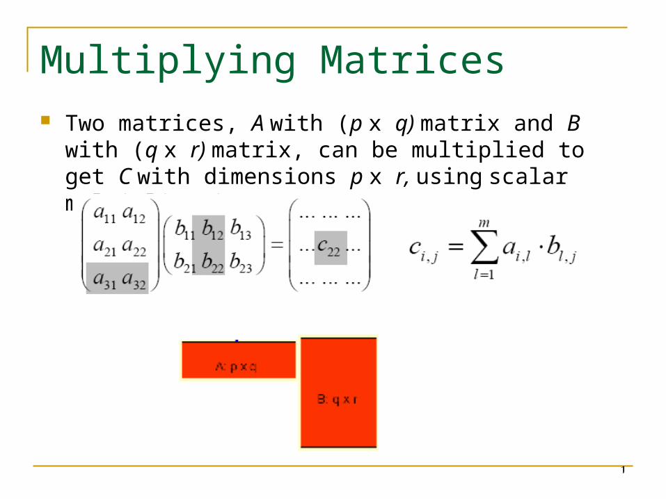
Multiplying Matrices Two matrices A with (p x q) matrix and B with (q x r)
matrix can be multiplied to get C with dimensions p x r using scalar multiplications
2
Multiplying Matrices
3
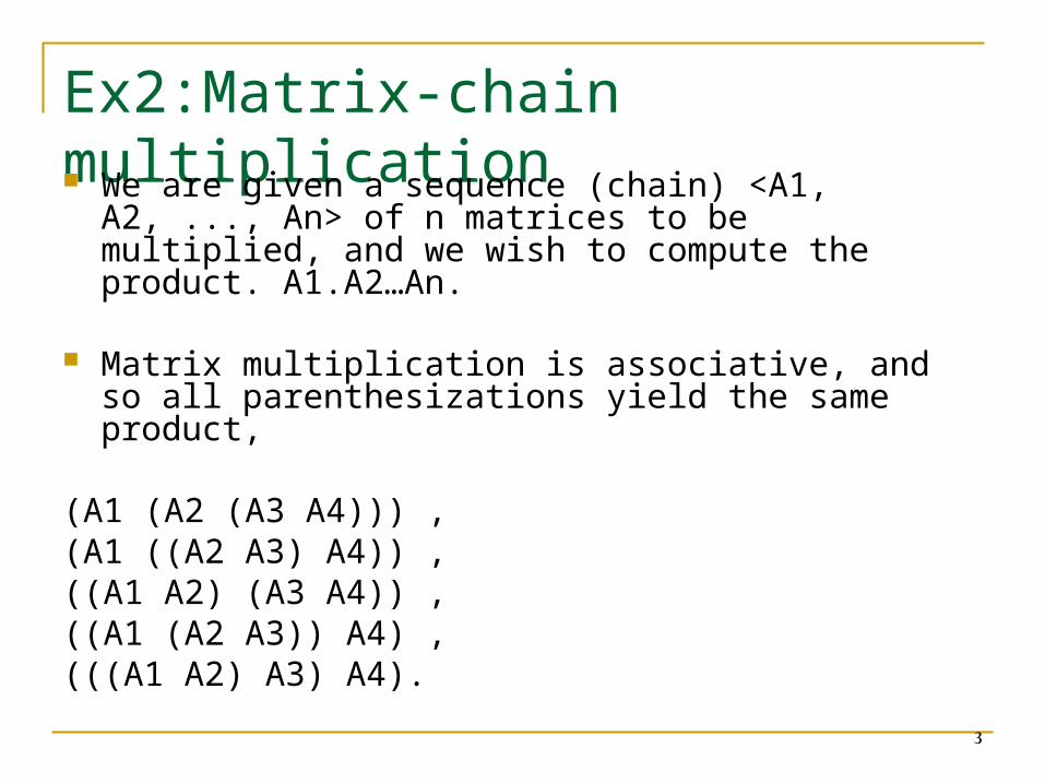
Ex2Matrix-chain multiplication We are given a sequence (chain) ltA1 A2 Angt of n
matrices to be multiplied and we wish to compute the product A1A2hellipAn
Matrix multiplication is associative and so all parenthesizations yield the same product
(A1 (A2 (A3 A4))) (A1 ((A2 A3) A4)) ((A1 A2) (A3 A4)) ((A1 (A2 A3)) A4) (((A1 A2) A3) A4)
4
Matrix-chain multiplication ndash cont
We can multiply two matrices A and B only if they are compatible the number of columns of A must equal the number of rows of B If A is a p times q matrix and B is a q times r matrix the resulting matrix C is a p times r matrix
The time to compute C is dominated by the number of scalar multiplications which is p q r
5
Matrix-chain multiplication ndash cont Ex consider the problem of a chain ltA1 A2 A3gt of
three matrices with the dimensions of 10 times 100 100 times 5 and 5 times 50 respectively
If we multiply according to ((A1 A2) A3) we perform 10 middot 100 middot 5 = 5000 scalar multiplications to compute the 10 times 5 matrix product A1 A2 plus another 10 middot 5 middot 50 = 2500 scalar multiplications to multiply this matrix byA3 for a total of 7500 scalar multiplications
If instead we multiply as (A1 (A2 A3)) we perform 100 middot 5 middot 50 = 25000 scalar multiplications to compute the 100 times 50 matrix product A2 A3 plus another 10 middot 100 middot 50 = 50000 scalar multiplications to multiply A1 by this matrix for a total of 75000 scalar multiplications Thus computing the product according to the first parenthesization is 10 times faster
6
Matrix-chain multiplication ndash cont Matrix multiplication is associative
q (AB)C = A(BC)
The parenthesization matters Consider A X B X C X D where
A is 30x1 B is 1x40 C is 40x10 D is 10x25
Costs ((AB)C)D = 1200 + 12000 + 7500 = 20700 (AB)(CD) = 1200 + 10000 + 30000 = 41200 A((BC)D) = 400 + 250 + 750 = 1400
7
Matrix Chain Multiplication (MCM) Problem Input
Matrices A1 A2 hellip An each Ai of size pi-1 x pi
Output Fully parenthesised product A1 x A2 x hellip x An
that minimizes the number of scalar multiplications
Note In MCM problem we are not actually multiplying
matrices Our goal is only to determine an order for
multiplying matrices that has the lowest cost
8
Matrix Chain Multiplication (MCM) Problem Typically the time invested in determining
this optimal order is more than paid for by the time saved later on when actually performing the matrix multiplications
So exhaustively checking all possible parenthesizations does not yield an efficient algorithm
9
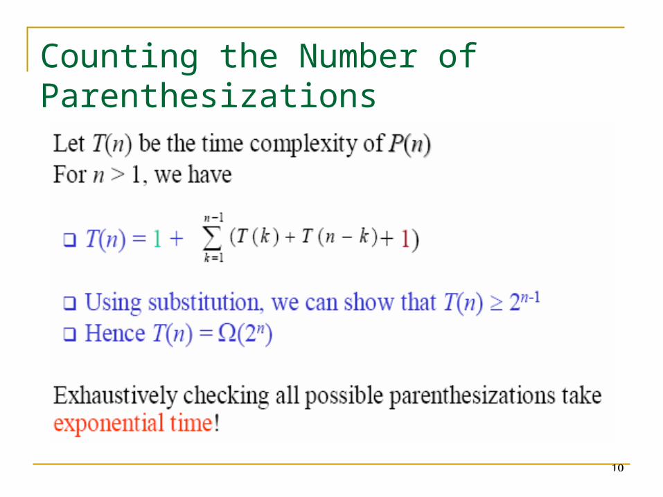
Counting the Number of Parenthesizations Denote the number of alternative parenthesizations of a
sequence of (n) matrices by P(n) then a fully parenthesized matrix product is given by
1048709 (A1 (A2 (A3 A4))) 1048709 (A1 ((A2 A3) A4)) 1048709 ((A1 A2) (A3 A4)) 1048709 ((A1 (A2 A3)) A4) 1048709 (((A1 A2) A3) A4)
If n = 4 ltA1A2A3A4gt then the number of alternative parenthesis is =5 P(4) =P(1) P(4-1) + P(2) P(4-2) + P(3) P(4-3) = P(1) P(3) + P(2) P(2) + P(3) P(1)= 2+1+2=5P(3) =P(1) P(2) + P(2) P(1) = 1+1=2P(2) =P(1) P(1)= 1
10
Counting the Number of Parenthesizations
11
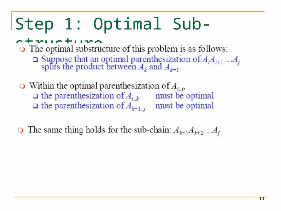
Step 1 Optimal Sub-structure
12
Step 1 Optimal Sub-structure
13
Step 1 Optimal Sub-structure
14
Step 1 Optimal Sub-structure
15
Step 2 Recursive Solution Next we define the cost of optimal solution
recursively in terms of the optimal solutions to sub-problems
For MCM sub-problems are problems of determining the min-cost of a
parenthesization of Ai Ai+1hellipAj for 1 lt= i lt= j lt= n
Let m[i j] = min of scalar multiplications needed to compute the matrix Aij For the whole problem we need to find m[1 n]
16
Step 2 Recursive Solution Since Aij can be obtained by breaking it into
Aik Ak+1j We have (each Ai of size pi-1 x pi) m[i j] = m[i k] + m[k+1 j] + pi-1pkpj
There are j-i possible values for k i lt= k lt= j
Since the optimal parenthesization must use
one of these values for k we need only check them all to find the best
17
Step 2 Recursive Solution
18
Step 3 Computing the Optimal Costs
19
Elements of Dynamic Programming
20
Overlapping Sub-problems
21
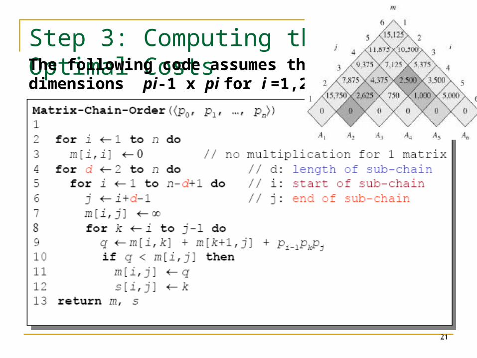
Step 3 Computing the Optimal CostsThe following code assumes that matrix Ai has dimensions pi-1 x pi for i =12 hellip n
22
Step 3 Computing the Optimal Costs
23
Step 3 Computing the Optimal Costs
24
Step 3 Computing the Optimal Costs
25
Step 3 Computing the Optimal Costs
26
Step 3 Computing the Optimal Costs
27
Step 3 Computing the Optimal Costs
28
Step 4 Constructing an Optimal Solution Although Matrix-Chain-Order determines the
optimal number of scalar multiplications needed to compute a matrix-chain product it does not directly show how to multiply the matrices
Using table s we can construct an optimal solution
29
Step 4 Constructing an Optimal Solution
30
Step 4 Constructing an Optimal Solution
31
Step 4 Constructing an Optimal Solution
32
Step 4 Constructing an Optimal Solution

2
Multiplying Matrices
3
Ex2Matrix-chain multiplication We are given a sequence (chain) ltA1 A2 Angt of n
matrices to be multiplied and we wish to compute the product A1A2hellipAn
Matrix multiplication is associative and so all parenthesizations yield the same product
(A1 (A2 (A3 A4))) (A1 ((A2 A3) A4)) ((A1 A2) (A3 A4)) ((A1 (A2 A3)) A4) (((A1 A2) A3) A4)
4
Matrix-chain multiplication ndash cont
We can multiply two matrices A and B only if they are compatible the number of columns of A must equal the number of rows of B If A is a p times q matrix and B is a q times r matrix the resulting matrix C is a p times r matrix
The time to compute C is dominated by the number of scalar multiplications which is p q r
5
Matrix-chain multiplication ndash cont Ex consider the problem of a chain ltA1 A2 A3gt of
three matrices with the dimensions of 10 times 100 100 times 5 and 5 times 50 respectively
If we multiply according to ((A1 A2) A3) we perform 10 middot 100 middot 5 = 5000 scalar multiplications to compute the 10 times 5 matrix product A1 A2 plus another 10 middot 5 middot 50 = 2500 scalar multiplications to multiply this matrix byA3 for a total of 7500 scalar multiplications
If instead we multiply as (A1 (A2 A3)) we perform 100 middot 5 middot 50 = 25000 scalar multiplications to compute the 100 times 50 matrix product A2 A3 plus another 10 middot 100 middot 50 = 50000 scalar multiplications to multiply A1 by this matrix for a total of 75000 scalar multiplications Thus computing the product according to the first parenthesization is 10 times faster
6
Matrix-chain multiplication ndash cont Matrix multiplication is associative
q (AB)C = A(BC)
The parenthesization matters Consider A X B X C X D where
A is 30x1 B is 1x40 C is 40x10 D is 10x25
Costs ((AB)C)D = 1200 + 12000 + 7500 = 20700 (AB)(CD) = 1200 + 10000 + 30000 = 41200 A((BC)D) = 400 + 250 + 750 = 1400
7
Matrix Chain Multiplication (MCM) Problem Input
Matrices A1 A2 hellip An each Ai of size pi-1 x pi
Output Fully parenthesised product A1 x A2 x hellip x An
that minimizes the number of scalar multiplications
Note In MCM problem we are not actually multiplying
matrices Our goal is only to determine an order for
multiplying matrices that has the lowest cost
8
Matrix Chain Multiplication (MCM) Problem Typically the time invested in determining
this optimal order is more than paid for by the time saved later on when actually performing the matrix multiplications
So exhaustively checking all possible parenthesizations does not yield an efficient algorithm
9
Counting the Number of Parenthesizations Denote the number of alternative parenthesizations of a
sequence of (n) matrices by P(n) then a fully parenthesized matrix product is given by
1048709 (A1 (A2 (A3 A4))) 1048709 (A1 ((A2 A3) A4)) 1048709 ((A1 A2) (A3 A4)) 1048709 ((A1 (A2 A3)) A4) 1048709 (((A1 A2) A3) A4)
If n = 4 ltA1A2A3A4gt then the number of alternative parenthesis is =5 P(4) =P(1) P(4-1) + P(2) P(4-2) + P(3) P(4-3) = P(1) P(3) + P(2) P(2) + P(3) P(1)= 2+1+2=5P(3) =P(1) P(2) + P(2) P(1) = 1+1=2P(2) =P(1) P(1)= 1
10
Counting the Number of Parenthesizations
11
Step 1 Optimal Sub-structure
12
Step 1 Optimal Sub-structure
13
Step 1 Optimal Sub-structure
14
Step 1 Optimal Sub-structure
15
Step 2 Recursive Solution Next we define the cost of optimal solution
recursively in terms of the optimal solutions to sub-problems
For MCM sub-problems are problems of determining the min-cost of a
parenthesization of Ai Ai+1hellipAj for 1 lt= i lt= j lt= n
Let m[i j] = min of scalar multiplications needed to compute the matrix Aij For the whole problem we need to find m[1 n]
16
Step 2 Recursive Solution Since Aij can be obtained by breaking it into
Aik Ak+1j We have (each Ai of size pi-1 x pi) m[i j] = m[i k] + m[k+1 j] + pi-1pkpj
There are j-i possible values for k i lt= k lt= j
Since the optimal parenthesization must use
one of these values for k we need only check them all to find the best
17
Step 2 Recursive Solution
18
Step 3 Computing the Optimal Costs
19
Elements of Dynamic Programming
20
Overlapping Sub-problems
21
Step 3 Computing the Optimal CostsThe following code assumes that matrix Ai has dimensions pi-1 x pi for i =12 hellip n
22
Step 3 Computing the Optimal Costs
23
Step 3 Computing the Optimal Costs
24
Step 3 Computing the Optimal Costs
25
Step 3 Computing the Optimal Costs
26
Step 3 Computing the Optimal Costs
27
Step 3 Computing the Optimal Costs
28
Step 4 Constructing an Optimal Solution Although Matrix-Chain-Order determines the
optimal number of scalar multiplications needed to compute a matrix-chain product it does not directly show how to multiply the matrices
Using table s we can construct an optimal solution
29
Step 4 Constructing an Optimal Solution
30
Step 4 Constructing an Optimal Solution
31
Step 4 Constructing an Optimal Solution
32
Step 4 Constructing an Optimal Solution

29
Step 4 Constructing an Optimal Solution
30
Step 4 Constructing an Optimal Solution
31
Step 4 Constructing an Optimal Solution
32
Step 4 Constructing an Optimal Solution

30
Step 4 Constructing an Optimal Solution
31
Step 4 Constructing an Optimal Solution
32
Step 4 Constructing an Optimal Solution

31
Step 4 Constructing an Optimal Solution
32
Step 4 Constructing an Optimal Solution

32
Step 4 Constructing an Optimal Solution