1 nearest neighbor classification for high-speed big...
TRANSCRIPT

1
Nearest Neighbor Classification for High-Speed BigData Streams Using Spark
Sergio Ramırez-Gallego, Bartosz Krawczyk, Salvador Garcıa, Michał Wozniak, Jose Manuel Benıtez,and Francisco Herrera
Abstract
Mining massive and high-speed data streams is one of the main contemporary challenges in machine learning. It requiresmethods characterized by a high computational efficacy that are able to continuously update their structure and handle ever-arriving big volumes of instances. In this paper we present a new incremental and distributed classifier based on the popularNearest Neighbor algorithm, adapted to such a demanding scenario. This method, implemented in Apache Spark, includes adistributed metric-space ordering to perform faster searches. Additionally, we propose an efficient incremental instance selectionmethod for massive data streams that continuously updates and removes outdated examples from the case-base. This allowedus to alleviate the high computational requirements of the original classifier and make it suitable for the considered problem.Experimental study conducted on a set of real-life massive data streams proves the usefulness of the proposed solution and showsthat it is able to provide the first efficient Nearest Neighbor solution for high-speed big and streaming data.
Index Terms
machine learning, data streams, big data, instance reduction, nearest neighbor, distributed computing, Apache Spark.
I. INTRODUCTION
The massive volume of information gathered by contemporary systems became omnipresent, as many research activitiesrequire collecting increasingly huge amounts of data. For instance, Large Hadron Collider experiments1 generates 30 petabytesof information per year. Potential applications for massive data analysis techniques could be found in each human activitydomain. Enterprises would like to discover interesting client behavior characteristics, e.g., on the basis of sensor or Internetdata. Another example would be works on personalized medical treatment for individual patients based on his/her clinicalrecords, such as medical history, genomic, cellular, and environmental data.
The contemporary man is surrounded by enormous volumes of data arriving continuously from different sources, therefore onemay say that we are living in the big data era. Big data is usually characterized by the so-called 5V’s (Volume, Velocity, Variety,Veracity, and Value), which describe its massive volume, dynamic nature, diverse forms, different qualities and usefulness forhuman [1].
In many cases we do not deal with static data collections, but rather with dynamic ones. They arrive in a form of continuousbatches of data, called data streams [2]. In such scenarios we need not only to manage the volume, but also the velocity ofdata, constantly updating our learning model and adapting it to the current state of the stream. To add a further difficulty, manymodern data sources generate their outputs with very short intervals, thus leading to high-speed data streams [3]. In this workwe will mainly focus on two characteristic of the big data, i.e., volume and velocity.
Massive data must be explored efficiently and converted into valuable knowledge which could be used by enterprises (amongothers) to build their competitive advantage [4]. However, there exist a considerable gap between contemporary processingand storage capacities that demonstrate our ability to capture and store data has far outpaced our ability to process and utilizeit. Moore’s law says that processing capacity double every 18 months, while disk storage capacity doubles every 9 months(storage law) [5]. It could cause that so-called data tombs, i.e., volume of data which are stored but never analyzed, mayappear. Therefore, we have to develop dedicated tools and techniques which are able to analyze enormous volume of incomingdata and additionally to take into consideration that each record may be analyzed only once to reduce the overall computingcosts [6]. MapReduce was the first programming paradigm in dealing with the phenomenon of big data, introduced in 2003 [7].Recently, a new large-scale processing framework, called Apache Spark [8], [9], is gaining importance in the big data domaindue to its good performance in iterative and incremental procedures.
Lazy learning [10] (also called instance-based learning) is considered as one of the simplest and most effective schemesin supervised learning [11], in which generalization is deferred until a query is made to the case-base. However, as distancebetween every pair of cases must be computed (quadratic complexity), these methods tends to have much slower classification
S. Ramırez-Gallego, S. Garcıa, Jose Manuel Benıtez, and F. Herrera are with Department of Computer Science and Artificial Intelligence of the Universityof Granada, Granada, Spain, 18071. E-mails: {sramirez, salvagl, j.m.benitez, herrera}@decsai.ugr.es
B. Krawczyk is with the Department of Computer Science, Virginia Commonwealth University, Richmond, VA, 23284, USA. E-mail: [email protected]. Wozniak is with the Department of Computer Science, Wrocław University of Technology, Wyb. Wyspianskiego 27, 50-370 Wrocław, Poland. E-mail:
1http://home.cern/about/computing

2
phase than their counterparts. Furthermore, lazy learners, as k-Nearest Neighbor (k-NN), tend to accumulate instances whendata arrives in stream form, what causes that data related to the outdated concepts may still be used to make a decision.Because of these reasons lazy learning has not been widely used in streaming environments in spite of its attractive properties.
Data reduction techniques may be applied to improve the performance of lazy learners [12]. Concretely, instance selectiontechniques can be very effective as they aim at reducing the total number of samples stored in the case-base and thereforethe underlying search space. Search speed may also be improved by introducing an implicit metric-space ordering in thecase-base [13] or through other techniques as locality-sensitive hashing [14].
In this work, we propose an efficient nearest neighbor solution to classify fast and massive data streams using ApacheSpark. It consists of a distributed case-base and an instance selection method that enhances its performance and effectiveness.A distributed metric tree has been designed to organize the case-base and consequently to speed up the neighbor searches. Thisdistributed tree consists of a top-tree (in the master node) that routes the searches in the first levels and several leaf nodes (inthe slaves nodes) that solve the searches in next levels through a completely parallel scheme. Performance is further improvedby a distributed edition-based instance selection method, which only inserts correct examples and removes the noisy ones.Up to the best of our knowledge, this is the first lazy learning solution in dealing with large-scale, high-speed and streamingproblems.
The main contributions of this work are as follow:• Efficient and scalable incremental nearest neighbor classification scheme for massive and high-speed data streams.• Smart partitioning of the incoming data streams to parallelize the proposed algorithm using Spark environment.• Embedded instance selection method with quickly updated hybrid trees.• Comprehensive experimental evaluation of the proposed methods.Experimental results performed using several datasets and configurations show that our proposal outperforms the same
model without edition in terms of accuracy. Our method also reduces the time spent in the prediction stage and the memoryconsumption.
The structure of the work is as follows. Firstly, the related works about big data analysis, data stream mining, nearestneighbor and instance selection are presented in Section II. Then the proposed solution for Spark architecture is discussed inSection III. The next section (Section IV) includes results of experimental investigation. Lastly, Section V concludes the work.
II. RELATED WORKS
This section will provide necessary background on recent advances in mining massive (Section II-A) and streaming datasets(Section II-B), with special focus put on nearest neighbor based classification approach (Section II-C).
A. Big data analytics
As we mentioned above we require efficient and scalable analytic methods to deal with massive data.Google designed MapReduce [7] in 2003, which is considered as one of the first distributed frameworks for large-scale
processing. MapReduce is aimed at automatically processing data in an easy and transparent way through a cluster of computers.The user only needs to implement two operators: Map and Reduce. In the Map phase, the system processes key-value pairsread directly from a distributed file system and transform them into another set of pairs (intermediate results). Each node is incharge of reading and transforming a set of pairs from one or more data partitions. In the Reduce phase, the key coincidentpairs are sent to the same node and merged to yield the final result through an user-defined function. For further informationabout MapReduce and others distributed frameworks, please check [6].
Apache Hadoop [15], [16] is an open-source implementation of MapReduce for reliable, scalable, and distributed computing.Despite its popularity and it has been used to develop several mining techniques [17], [18], Hadoop is not suitable for manyscenarios specially those where the user explicitly re-uses data. For instance, online, interactive and/or iterative computing [19]are affected by this problem.
Apache Spark [8], [9] is a distributed computing platform that has become one of the most powerful engines in the bigdata scenario. According to its creators, this platform was designed to overcome the problems of Hadoop. In fact, the Sparkengine has shown to perform faster than Hadoop in many cases (up to 100x in memory). Thanks to its in-memory primitives,Spark is able to load data into memory and query it repeatedly, making it suitable for iterative processes (e.g. machine learningalgorithms). In Spark, the driver (the main program) controls multiple workers (slaves) and collects results from them, whereasworker nodes read data blocks (partitions) from a distributed file system, perform some computations and save the result todisk.
Resilient Distributed Dataset (RDD) is the base structure in Spark, on which the distributed operations are performed. A widevariety of operations are offered by RDDs, such as: filtering, mapping, and joining large data. These operations are designed totransform datasets by locally executing tasks within the data partitions, thus maintaining the data locality. Furthermore, RDDsare a versatile tool that allows programmers to preserve intermediate results (in memory and/or disk) in several formats forre-usability purposes, as well as customize the partitioning for data placement optimization.

3
Spark also allows us to use the RDD’s API in streaming environments through the transformation of data streams into smallbatches. Spark Streaming’s design enables the same batch code (formed by RDD transformations) to be used in streaminganalytics with almost no change.
For large-scale machine learning, several common learning algorithms and statistic utilities were created and packaged intoMLlib [20], [21], the machine learning library of Spark. This library gives support to several knowledge discovery tasks suchas: classification, optimization, regression, collaborative filtering, clustering, and data pre-processing.
B. Data stream mining
Contemporary machine learning problems are often characterized not only by a significant volume of data, but also by itsvelocity. Instances may arrive continuously in a form of a potentially unbounded data stream [22]. This poses new challengesfor learning algorithms, as they must offer adaptation mechanisms to ever-growing dataset, being able to update their structurein accordance with the current state of a stream [23]. Additionally, new constraints must be taken into consideration that arenot present or not so important in static scenarios [24]. Learner must have low response and update times, as new objectsmust be handled as soon as they become available. Too long processing would cause a delay with stacking arriving objectsthat would only increase with the stream progress. Furthermore, streaming algorithms must assume limited storage space andmemory consumption. One cannot store all of objects from a stream, as data volume will continuously expand [25]. Therefore,objects should be discarded after processing and learner must not require an access to previously seen instances.
Data streams are often characterized by a phenomenon called concept drift [26], [27]. It can be defined as a change ofcharacteristic in incoming data over the course of stream processing.
In streaming environments [2], the incoming objects arrive sequentially, therefore data streams can be processed in twodifferent operation modes:
• Chunk (batch), where data either arrive in a form of instance blocks or we collect enough instances to form one.• Online, where instances arrive one by one and we must process them as soon as they become available.There are several possible approaches to learning from data streams:• Rebuilding the classifier whenever new data becomes available.• Using a sliding window approach.• Using an incremental or online learner.The first of discussed approaches is far from being applicable in real stream mining environment. Training a new model
whenever a new set of instances arrive would impose prohibitive computational costs and excessive need for a storage space inorder to accommodate the ever-growing size of the training set. Additionally, during the training process the classifier wouldbe unavailable for data processing, which would lead into a significant time delay. These factors force us to design specializedmethods that do not suffer from the mentioned limitations.
Sliding window-based classifiers were designed primarily for drifting data streams, as they incorporate the forgettingmechanism in order to discard irrelevant samples and adapt to the progress of incoming stream [28]. Recent works in this areaincorporate dynamic window size adjustment [29] or usage of multiple windows [30]. However, we focus on stationary datastreams for which proper and continuous model update is of greater importance. Therefore, let us discuss in more details thethird group of methods.
Incremental [31] and online [32] learners are such classifiers that are able to continuously update their structure or decisionboundaries according to incoming new data [33]. Such methods must meet several requirements, such as processing eachobject only once during the course of training, having strictly limited memory and time consumption, and their training canbe stopped at any time with obtained quality not lower than the one from corresponding classifier trained with the same datain a static mode [34]. Main advantages of such methods lie in their fast and flexible adaptation to new data, as they are notrebuilt from a scratch every time new instances become available. Additionally, once the object has been processed it can bediscarded as it will be of no future use for the classifier. This significantly reduce the requirement for memory and storagespace. It is worth noticing that some of popular classifiers can work in incremental or online mode, e.g., Naıve Bayes, NeuralNetworks or Nearest Neighbor methods. There is also a number of classifiers that have been specifically modified to workwith changing streams of instances, like Concept-Adapting Decision Trees [35] or Very Fast Decision Rules [36].
Nearest Neighbor algorithms are highly popular in traditional machine learning for their ease of implementation and provedhigh efficiency. However, due to their lazy learning nature and high computational costs they have not gained significantattention in the domain of data stream analysis [37], [38], especially when instances arriving with high speed are considered.Let us now review the most popular approaches for speeding-up this classifier.
C. Speeding-up nearest neighbor searches
k-NN [39] is an intuitive and effective non-parametric model used in many machine learning problems and can be consideredas one of top-ten most influential algorithms in data mining [40]. Nevertheless, k-NN is also a time-consuming method thatrequires all the training instances to be stored in memory and to compute the di/stance measurement between every pair of
4
instances (quadratic complexity). For this reason, a linear search becomes impractical when large-scale problems are facedand/or new examples are constantly introduced to the case-base.
Many techniques have been proposed to alleviate the k-NN search complexity. They range from metric trees [13], whichindex data through a metric-space ordering; to locally sensitive hashing [14], which map (with high probability) those elementsnear in the space to the same bins.
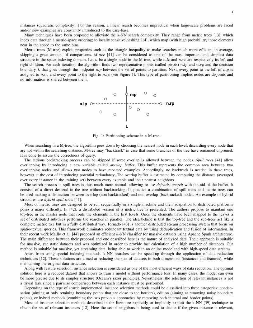
Metric trees (M-tree) exploit properties such as the triangle inequality to make searches much more efficient in average,skipping a great amount of comparisons. M-tree [41] can be considered as one of the most important and simplest datastructure in the space-indexing domain. Let n be a single node in the M-tree, while n.lc and n.rc are respectively its left andright children. For each iteration, the algorithm finds two representative points (called pivots) n.lp and n.rp and the decisionboundary L that goes through the midpoint mp between the set of points to partition. Next, every point to the left of mp isassigned to n.lc, and every point to the right to n.rc (see Figure 1). This type of partitioning implies nodes are disjoints andno information is shared between them.
Fig. 1: Partitioning scheme in a M-tree.
When searching in a M-tree, the algorithm goes down by choosing the nearest node in each level, discarding every node thatare not within the searching distance. M-tree may ”backtrack” in case that some branches of the tree have remained unpruned.It is done to assure the correctness of query.
The tedious backtracking process can be skipped if some overlap is allowed between the nodes. Spill trees [41] allowoverlapping by introducing a new variable called overlap buffer. This buffer represents the common area between twooverlapping nodes and allows two nodes to have repeated examples. Accordingly, no backtrack is needed in these trees,however at the cost of introducing potential redundancy. The overlap buffer is estimated by computing the distance (averagedover every instance in the training set) between every example and their nearest neighbors.
The search process in spill trees is thus much more natural, allowing to use defeatist search with the aid of the buffer. Itconsists of a direct descend in the tree without backtracking. In practice a combination of spill trees and metric trees canbe used making a distinction between overlap (non-backtracked) and non-overlap (backtracked) nodes. An example of hybridstructures are hybrid spill trees [41].
Most of metric trees are designed to be run sequentially in a single machine and their adaptation to distributed platformsposes a major difficulty. In [42], a distributed version of a metric tree is presented. The authors propose to maintain onetop-tree in the master node that route the elements in the first levels. Once the elements have been mapped to the leaves aset of distributed sub-trees performs the searches in parallel. The idea behind is that the top-tree and the sub-trees act like acomplete metric tree but in a fully distributed way. Tornado [43] is another distributed stream processing system that focus onspatio-textual queries. This framework eliminates redundant textual data by using deduplication and fusion of information. Intheir recent work Maillo et al. [44] proposed an efficient k-NN classifier for massive datasets using Apache Spark architecture.The main difference between their proposal and one described here is the nature of analyzed data. Their approach is suitablefor massive, yet static datasets and was optimized in order to provide fast calculation of a high number of distances. Ourmethod is suitable for massive, yet streaming data, being able to work in an online mode and with high-speed data streams.
Apart from using special indexing methods, k-NN searches can be speed-up through the application of data reductiontechniques [12]. These solutions are aimed at reducing the size of datasets in both dimensions (instances and features), whilemaintaining the original data structure.
Along with feature selection, instance selection is considered as one of the most efficient ways of data reduction. The optimalsolution here is a reduced dataset that allows to train a model without performance loss. In many cases, the model can evenbe more precise due to its simpler structure (Occam’s razor principle). Nevertheless, the selection of relevant instances is nota trivial task since a pairwise comparison between each instance must be performed.
Depending on the type of search implemented, instance selection methods could be classified into three categories: conden-sation (aiming at only retaining boundary points that are close to the borders), edition (aiming at removing noisy boundarypoints), or hybrid methods (combining the two previous approaches by removing both internal and border points).
Most of instance selection methods described in the literature explicitly or implicitly exploit the k-NN [39] technique toobtain the set of relevant instances [12]. Here the set of neighbors is being used to decide if the given instance is relevant,

5
redundant or noisy according to a determined criterion. Classical selection methods as Reduced-NN, Edited-NN (ENN) orCondensed-NN, make use of NN technique to evaluate instances. However, there are many other selection algorithms that useother measures as accuracy, retrieval frequency, or competence. For instance, the Iterative Case Filtering (ICF) method removesthose instances whose reachability (instances that are correctly solved by a given element) is less than its coverage (instancesthat correctly solved a given element). However, it is worth noticing that ICF launches ENN to remove noisy instances at thebeginning.
Relative Neighborhood Graph Edition (RNGE) algorithm [45]deserves a special attention. It is considered as one of themost accurate methods according to the experiments performed in [12]. In RNGE, the neighbors of an element are determinedby a special proximity graph called relative neighborhood graph. Two points are considered as neighbors in the graph if thereexist a connecting edge between them. The rule that determines this association is defined as: there exist an edge between twogiven points if there does not exist a third point that is closer to any of them than they are to each other. After building agraph the algorithm removes those instances misclassified by their neighbors (majority voting). RNGE is also remarkable byits efficiency since the graph can be constructed efficiently in O(nlog(n)) time [46].
III. DS-RNGE: AN SPARK-BASED INSTANCE SELECTION FRAMEWORK FOR NEAREST NEIGHBOR STREAM MINING
In this section, we present a lazy learning solution for massive data streams. DS-RNGE consists of a distributed case-base,and an instance selection method that enhances its performance and effectiveness. Our case-base is structured using a distributedmetric tree, which is entirely maintained in memory to expedite further neighbor queries. Note that not only neighbor queriesbut our complete scheme is based in-memory primitives from Spark. The source code of the complete project can be foundin: https://github.com/sramirez/spark-IS-streaming.
DS-RNGE proceeds in two phases for each newly arrived batch of data:• an edition/update phase aimed at maintaining and enhancing the case-base.• a prediction phase that classifies new unlabeled data.Both phases require fast neighbor queries to accomplish their mission. To deal with this problem, we propose a smart
partitioning of the input space in which each subtree queries only a single space partition. This scheme will allow us toparallelize the querying process across the cluster.
A single top-level tree is maintained in the master node to route the elements in the first levels where the partitioning is stillcoarse-grained. For each instance, the nearest element in the leaves in the top-tree is returned. The correspondence betweenleaf nodes and subtrees determines the local tree where the query will be performed (see Section II-C for further details).
As mentioned before, hybrid spill trees use backtracking and redundancy to deal with classification in borders which impliesa cost in time and memory that is far from acceptable in streaming applications. Our idea is to allow classification errorsnear borders in order to increase the computational efficiency. When the number of elements is much greater than the numberof partitions, the number of instances with neighbors in a different partition and the classification error derived from thisphenomenon become negligible. Defeatist search is used as reference for our model because of its outstanding performance.
Since an ever-growing and noisy case-base is unacceptable, an instance selection method that reduces the number of caseshas been introduced in our approach. A improved local version of RNGE has been applied to control the insertion and removalof noisy instances because of its competitive performance and effectiveness. The original method has been re-designed forincremental learning from data streams. For each incoming example, a relative graph is built around the instance and a subsetof neighbors. The local graphs are then used to edit the case-base by deciding what instances should be inserted, removed orleft untouched. As every step in this process is performed locally, the communication overhead is negligible.
DS-RNGE manages the following parameters:• nt: Number of sub-trees and number of leaf nodes in the top-tree.• ks: Number of neighbors used to build the local graphs (instance selection phase).• kp: Number of neighbors used in the prediction phase.• ro: Indicates whether removal of examples should be performed or not.Although edition in our system is guided by class, resulting case-bases can be employed in other learning processes with
tangible benefits. For instance, polished case-bases can work with semi-supervised or clustering [47], [48] problems. In general,noise removal should ease learning in other family of classifiers, like decision trees or statistical-based learners. As future work,we will study the effect of case-base edition on other classification methods.
In the following sections, we present the different procedures involved in DS-RNGE. Firstly, we describe the first steps toinitialize the distributed case-base (Section III-A). Afterwards, the editing/updating process is presented (Section III-B). Here,we present details of insertion and deletion of examples in the tree. Finally, in Section III-C we describe the prediction phase.
A. Initial partitioning process
The first step in our system consists of building a distributed metric tree formed by a top-tree in the master machine anda set of local trees in the slave machines. This distributed tree will be queried and updated during next iterations with new

6
incoming batches. From the first batch we take a sample of nt instances to build the main tree. The sampled data should besmall enough to fit in a single machine and should maximize the separability between examples to avoid overlapping in thefuture subtrees. The nt parameter is normally set to a value equal to the number of cores in the cluster. By doing so ouralgorithm is able to fully exploit the maximum level of parallelism in any stage. The routing tree is created following thestandard procedure presented in [41], where upper and lower bounds are defined to control the size of nodes.
Once the top-tree is initialized, it is replicated to each machine and one subtree per leaf node is created in the slave machines(line 7). Then, every element in the first batch is inserted in the subtrees following these steps:
• For each element, the algorithm searches the nearest leaf node in the top-tree. According to the correspondence betweenleaf nodes and subtrees we can determine to which subtree each element will be sent. This process is performed in a Mapphase.
• The elements are shuffled to the subtrees according to their keys. Each subtree gets a list of elements to be inserted.• For each subtree all received elements are inserted to the tree in a local way. This process is performed in a Reduce phase.Note that the partitions/subtrees derived from this phase will be maintained during the complete process for re-usability
purposes, so that only the arriving instances will be moved across the network in each iteration. Algorithm 1 explains thisprocedure in detail using a MapReduce syntax.
Algorithm 1 Initial partitioning process.
1: INPUT: data, nt2: // data is the input dataset3: // nt Number of leaf trees to be distributed across the nodes4: sample = smartSampling(data)5: topTree = In the master machine, build the top M-tree using sample and the standard partitioning procedure explained
in [41]. It will be replicated to every slave machine.6: For each leaf node in the topTree, one subtree is created in a single slave machine. The resulting set of trees (stored as
an RDD) is partitioned and cached for further processing.7: mapReduce e ∈ data8: Find the nearest leaf node to e in topTree, and outputs a tuple with the tree’s ID (key) and e (value). (MAP)9: The tuple is sent to the correspondent partition and attached to the subtree according to its key. (SHUFFLE)
10: Combine all the elements with the same key (tree ID) by inserting them into the local tree. (REDUCE)11: Return the updated tree.12: end mapReduce
B. Updating process with edition
When a new batch of data arrives the updating process with edition is being launched in our system. This process is aimed atinserting new correct examples, as well as removing those redundant examples already inserted. At first, the algorithm computeswhich subtree each element falls into following the same process described in the previous section. Once all instances areshuffled to the subtrees, a local nearest neighbor search for each element is started in corresponding sub-trees.
After obtaining neighbors the instance selector creates groups where each one is formed by a new element and its neighbors.Then, local RNGE is applied on each group (as explained in Algorithm 3). The idea behind that is to build a local grapharound each group and through this graph to decide what kind of action to perform on each element (insertion, removal ornone). New examples can be inserted or not, whereas old examples (neighbors) can be removed or maintained.
Since each graph only has a narrow view of the case-base the set of neighbors that can be removed has been limited tothose that share an edge with the new element. Removal of old examples can be controlled through the binary parameter ro.If activated, the removal may cause a drop in the overall accuracy but the prediction process will run faster because of thereduced size. Note that the insertion process is exact in most of cases since the new elements are in the center of the graphand a suitable number of neighbors (a default value of 10) is enough to find their edges. The number of neighbors for graphconstruction can be controlled through the ks parameter. The greater the value of ks, the more precise is the removal and theslower the process.
Once decisions for each element are taken we perform insertions and removals locally in the subtrees in the same reducephase. Notice that by doing so the neighbor query and the editing process are both performed in the same MapReduce process,thus reducing the communication overhead. The complete editing process is described in Algorithm 2.
Figure 2 illustrates all the steps involved in DS-RNGE for one training iteration (one batch). The first part shows how thetop-tree is built with two examples: e1 and e2. Once the main tree is built one sub-tree per element in the leaves is created inthe slave nodes. Every element is also inserted in its local subtree. In the second phase a new element e3 arrives at the top-tree.The top-tree routes the search to the first partition, where the element is sent to perform a neighbor search. This search willallow to decide if the element should be inserted or not. Let suppose that the edition method decides the insertion is suitable

7
Algorithm 2 Updating process with edition.
1: INPUT: query, ks, ro2: // query is the data to be queried3: // ks represents the number of neighbors to use in the instance selection phase.4: // ro indicates whether to remove old noisy examples or not.5: mapReduce e ∈ data6: Find the nearest leaf node to e in topTree and outputs a tuple with the tree’s ID (key) and e (value). (MAP)7: The tuple is sent to the correspondent subtree according to its key. (SHUFFLE)8: neighbors = the standard M-tree search process is launched for each element in its local subtree in order to retrieve
the ks-neighbors of e. The output will consist of a tuple with e (key) and a list of its ks-neighbors (value). (REDUCE)9: edited = apply the local RNGE algorithm (Algorithm 3) to each tuple in neighbors. The output consist of the
insertion/removal decision for each element.10: if ro == true then11: Removed old noisy instances in edited from the tree.12: end if13: Add new correct instances in edited to the tree.14: Return the updated tree.15: end mapReduce
Algorithm 3 Local RNGE.
1: INPUT: e, ne2: // e incoming example3: // ne set of neighbors for e4: Compute the local RNGE graph using e and ne following the procedure detailed in [46].5: Mark e to be added iff most of its graph neighbors agree with its class6: for en ∈ ne do7: if en is a graph neighbor of e and most of en’s graph neighbors do not agree with its class then8: Mark en to be removed9: end if
10: end for
according to its nearest neighbor (1-NN) (in this case, e1). The insertion is then fully local as the element has been alreadysent to the correspondent node and partition. The removal process performs the same operations but removing those cases thatdo not agree with the edition results. In this case the decision for e1 is to remain unchanged.
Fig. 2: Flowchart describing initialization, searching and insertion processes in DS-RNGE.
Within the edition process, local construction of graphs and subsequent filtering is depicted in Figure 3. In this graphic anew example from class A (dashed point) arrives to a given partition (Algorithm 2). From the set of points in that partition,ks = 4-NN (thick circles) are selected from the pool to construct the graph shown in step 2. Note that graphs are built

8
independently from other cases in the partition. Lastly, removal decisions are made according to the connections betweenneighbors. In our example, the dashed example is not inserted in the case-base since most of its edge-neighbors do not agreewith its class. As there not exist more agreements between nodes, no more removals are accomplished.
Fig. 3: Local graph edition for each new example. Class A is coloured in red, and class B in blue
C. Prediction processClassification process is an approximate function that is started when new unlabeled data arrive at the system (see Algo-
rithm 4). For each element the algorithm searches for the nearest leaf node in the master node and shuffles the elements tothe slave machines. Next, the standard M-tree search process is used to retrieve the kp-neighbors of each new element. Foreach group, formed by a new element and its neighbors, the algorithm predicts the element’s class by applying the majorityvoting scheme to its neighbors. Notice that the query and the prediction are both performed in the same MapReduce phase asin the edition process.
Algorithm 4 Prediction process.
1: INPUT: query, kp2: // query is the data to be queried3: // kp represents the number of neighbors for predictions.4: mapReduce e ∈ data5: Find the nearest leaf node to e in topTree and outputs a tuple with the tree’s ID (key) and e (value). (MAP)6: The tuple is sent to the correspondent subtree according to its key. (SHUFFLE)7: neighbors = the standard M-tree search process is launched for each element in its local subtree in order to retrieve
the ks-neighbors of e. The output will consist of a tuple with e (key) and a list of its ks-neighbors (value). (REDUCE)8: For each tuple in neighbors return the most-voted class from the list of neighbors. This value will be the class predicted
for the given element.9: end mapReduce
IV. EXPERIMENTAL STUDY
In order to evaluate the proposed methods we have designed a thorough experimental study with the following goals inmind:
• To evaluate the quality and performance of DS-RNGE versus the base model without edition, as well as to check theeffect of the batch size on the models (Section IV-B).
• To check if defeatist search really affects the precision and processing time in tree queries. To do that we perform acomparison between the edited models and the base model without edition (Section IV-C).
• To validate that our model scales-out correctly by increasing the number of cores available in the cluster (Section IV-D).
A. Experimental FrameworkFive large-scale datasets (poker, susy, hhar2, hepmass and higgs) from the UCI Machine Learning Database Repository [49]
and another big dataset (called ECBDL14) have been used to evaluate the performance and quality of DS-RNGE. ECBDL143 is
2From the Heterogeneity Human Activity Recognition experiment, only the activity recognition dataset was used3http://cruncher.ncl.ac.uk/bdcomp/

9
a highly-imbalanced problem derived from the data mining competition held under the International Conference GECCO-2014.A random sampling without replacement (25% of the original size) was applied to ECBDL14 and hhar datasets.
In order to transform these static datasets into streams they were randomly partitioned into equal-sized data batches accordingto different batch sizes (50, 000, 100, 000 and 200, 000). Before the start of executions, the batches are enqueued. Only onebatch per iteration (one second) serves as an input to our system. To prevent the insertion of repeated instances in the metrictrees the unique examples from these datasets were extracted and used as the former input for the models. In Table I, all thedetails about the datasets included in our experiments are presented.
TABLE I: Datasets used in the experiments (summary description). For each set, the number of original examples (# Inst.),the number of unique examples (# Unique), the total number of attributes (#Atts.), and the number classes (#Cl) are shown.
Data Set # Inst. # Unique #Atts. #Cl.
poker 1,025,009 1,022,770 10 10susy 5,000,000 5,000,000 18 2hhar (25%) 7,535,705 7,535,705 7 7ecbdl14 (25%) 7,994,298 7,994,298 10 2hepmass 10,500,000 10,500,000 28 2higgs 11,000,000 10,721,302 28 2
Regarding the evaluation process, DS-RNGE is first tested with the current batch in the queue and then updated with it.This streaming evaluation process is called interleaved test-then-train model [50] and allows us to always test our model onunseen examples.
In our experiments three models have been tested. The first one, called edited, follows the DS-RNGE scheme presented inSection IV-A, but without allowing the removal of already inserted examples. The second method, called edited-re, is anotherversion of DS-RNGE but with removal. And as benchmark method, the same distributed scheme is used but without any typeof edition. This scheme, called orig, directly inserts elements in the distributed trees and apply the usual prediction process(explained in Algorithm 4).
TABLE II: Parameters of the distributed models.
Method Parameters
edited (DS-RNGE) nt = 420, ks = 10, kp = 1, ro = falseedited-re (DS-RNGE) nt = 420, ks = 10, kp = 1, ro = trueorig nt = 420, ks = 0 (no edition), kp = 1, ro = false
The experiments were performed on a cluster composed of twenty standard nodes (hosting the Spark workers) and one master(hosting the Spark Master) node. The computing nodes have the following features: 2 processors x Intel Xeon CPU E5-2620 (6cores/processor, 2.00 GHz, 15 MB cache), 2 TB HDD, 64 GB RAM. They are connected through a QDR InfiniBand network(40 Gbps). The following software was used in the experiments: Hadoop 2.5.0-cdh5.3.1 from Cloudera’s open-source ApacheHadoop distribution4, HDFS replication factor: 2, HDFS default block size: 128 MB, Apache Spark Streaming 1.6, 460 cores(23 CPU cores/node), 960 RAM GB (48 GB/node). The datasets are hosted in the distributed file system, but they are loadedfrom memory, and cached there before starting the executions.
Let us now discuss in details the obtained results according to several criteria: the different batch sizes and edition strategies,the search strategy used in metric trees and the scalability of our method.
B. General comparison –evaluation of batch sizes and edition strategies
Detailed results for every dataset, model and batch size are given in Tables IV–VIII. For each combination, several informationfields are shown: the batch size, the method used, the average accuracy (Acc.), the average training time (Tr. time), the averageclassification time (Cls. time), the average number of instances and the percent of reduction in brackets (# Inst. (%)), and thetime (in seconds) spent in the whole process. The best result for each column is highlighted in bold.
From these experiments we can state the following conclusions: for every dataset, DS-RNGE without removal (edit) ismore precise than the other methods, which means that DS-RNGE is useful in enhancing case-bases. DS-RNGE with removal(edit-re) only obtains better results than the version without edition (orig) in two datasets: susy and ecbdl14. Competitiveresults in ecbdl14 can be explained by the fact that reduction is negligible in this dataset, whereas for susy, it is not clear if itis due to hypo-reduction or other factors. Note that both susy and hepmass benefits from the same level of reduction, however,reduction is proven to be much more negative in the last dataset. By other factors, we mean: incomplete graphs for insertedexamples, high dependency between removed instances and their potential incoming neighbors, or high noise in data.
4http://www.cloudera.com/content/cloudera/en/documentation/cdh5/v5-0-0/CDH5-homepage.html

10
It can be explained by the fact that the reduction rates in these two datasets were lower than ones for remaining benchmarks.Over-reducing the number of elements implies a natural loss of precision.
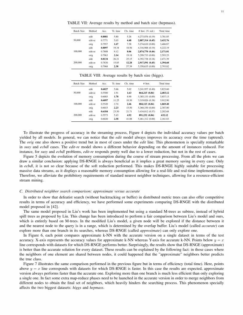
The edit model is not only precise but also offers highly satisfactory computational time, similar to the original version (thefastest option). In most of the cases, edit is characterized by better classification times than orig and similar results in totaltime. When the amount of reduced elements is low, orig is faster than edit (see Table VI). Nevertheless, when there is a clearreduction (Table VII), edit compensates its time-consuming training process with a quicker classification. On the other hand,there is a clear advantage in terms of time on using removal (method edit-re) but it fails on accuracy in 4/6 datasets.
200,000 elements per second seems to be the best batch size for all datasets. According to the results, it can be stated thatthe bigger the batch size, the lower the total time and the higher the average time (both classification and training). A biggerbatch size implies that less network communication and map/reduce phases are performed. However, as more data is used forinitialization with a bigger batch size the average reduction gets lower and the average time results higher.
TABLE III: Average results by method and batch size (poker).
Batch Size Method Acc. Tr. time Cls. time # Inst. (% red.) Total time
50,000edit 0.5418 2.47 1.97 330,433 (0.38) 76.65edit-re 0.5353 2.22 1.93 81,764 (0.85) 71.26orig 0.5351 2.34 1.69 537,233 (0.00) 73.61
100,000edit 0.5479 3.67 2.95 369,737 (0.34) 40.05edit-re 0.5368 3.33 2.90 86,242 (0.85) 38.10orig 0.5380 3.42 2.67 563,066 (0.00) 39.77
200,000edit 0.5599 5.52 3.81 445,614 (0.27) 10.82edit-re 0.5448 4.85 3.69 92,788 (0.85) 10.33orig 0.5495 4.48 4.58 614,467 (0.00) 9.72
TABLE IV: Average results by method and batch size (susy).
Batch Size Method Acc. Tr. time Cls. time # Inst. (% red.) Total time
50,000edit 0.7699 2.04 1.80 1,967,910 (0.22) 671.381edit-re 0.7565 1.80 1.59 1,068,652 (0.58) 629.076orig 0.7156 1.52 1.78 2,525,658 (0.00) 653.148
100,000edit 0.7691 3.63 3.21 1,999,418 (0.22) 281.50edit-re 0.7624 2.60 2.31 1,082,872 (0.58) 323.40orig 0.7160 1.90 4.16 2,551,471 (0.00) 246.67
200,000edit 0.7579 5.94 4.75 2,063,179 (0.21) 224.51edit-re 0.7678 4.96 3.96 1,124,473 (0.57) 188.68orig 0.7164 2.15 5.70 2,604,533 (0.00) 172.17
TABLE V: Average results by method and batch size (hhar).
Batch Size Method Acc. Tr. time Cls. time # Inst. (% red.) Total time
50,000edit 0.5595 1.87 1.56 2,101,474 (0.45) 1,263.19edit-re 0.4082 1.56 1.37 979,382 (0.74) 1,178.99orig 0.5414 1.59 1.77 3,793,085 (0.00) 1,268.03
100,000edit 0.5612 2.81 2.45 2,170,698 (0.43) 617.54edit-re 0.4694 2.28 2.06 1,078,336 (0.72) 549.50orig 0.5416 2.05 2.96 3,818,059 (0.00) 621.15
200,000edit 0.5564 5.29 4.07 2,260,555 (0.42) 364.42edit-re 0.4917 4.27 3.45 1,143,478 (0.70) 310.29orig 0.5449 2.29 5.13 3,869,666 (0.00) 307.91
TABLE VI: Average results by method and batch size (ECBDL14).
Batch Size Method Acc. Tr. time Cls. time # Inst. (% red.) Total time
50,000edit 0.9769 3.66 2.80 3,935,148 (0.02) 1,854.16edit-re 0.9780 5.09 3.69 3,686,600 (0.08) 2,192.86orig 0.9600 1.67 2.69 4,022,399 (0.00) 1,573.16
100,000edit 0.9767 8.54 6.72 3,960,385 (0.02) 1,384.63edit-re 0.9773 7.02 5.16 3,712,289 (0.08) 1,161.05orig 0.9599 2.00 4.25 4,047,791 (0.00) 751.88
200,000edit 0.9766 9.90 7.98 4,011,542 (0.02) 658.41edit-re 0.9785 13.56 10.11 3,764,620 (0.08) 832.44orig 0.9600 2.33 8.89 4,099,311 (0.00) 447.95
11
TABLE VII: Average results by method and batch size (hepmass).
Batch Size Method Acc. Tr. time Cls. time # Inst. (% red.) Total time
50,000edit 0.8081 5.80 5.26 4,273,076 (0.19) 3,781.85edit-re 0.7771 5.03 4.48 2,887,314 (0.45) 3,432.76orig 0.7957 1.67 7.58 5,274,610 (0.00) 3,466.87
100,000edit 0.8097 19.34 18.56 4,316,988 (0.19) 4,222.19edit-re 0.7808 9.12 8.06 2,874,770 (0.46) 2,171.01orig 0.7963 2.14 19.18 5,299,733 (0.00) 2,593.25
200,000edit 0.8134 26.21 25.15 4,392,738 (0.18) 2,471.39edit-re 0.7830 15.85 12.28 2,917,591 (0.45) 1,394.60orig 0.7968 2.38 57.39 5,350,635 (0.00) 2,793.82
TABLE VIII: Average results by batch size (higgs).
Batch Size Method Acc. Tr. time Cls. time # Inst. Total time
50,000edit 0.6027 5.66 5.02 3,241,957 (0.40) 3,823.60edit-re 0.5500 1.91 1.63 864,215 (0.84) 2,403.12orig 0.6003 1.78 8.90 5,385,153 (0.00) 3,857.13
100,000edit 0.6097 11.25 10.30 3,319,026 (0.38) 3,912.90edit-re 0.5549 2.74 2.46 884,123 (0.84) 1,069.40orig 0.6015 2.23 15.50 5,360,330 (0.00) 2,307.00
200,000edit 0.6184 23.50 21.71 3,434,012 (0.37) 2,202.68edit-re 0.5573 5.43 4.92 891,232 (0.84) 632.12orig 0.6020 2.58 41.08 5,461,312 (0.00) 2,161.83
To illustrate the progress of accuracy in the streaming process, Figure 4 depicts the individual accuracy values per batchyielded by all models. In general, we can notice that the edit model always improves its accuracy over the time (uptrend).The orig one also shows a positive trend but in most of cases under the edit line. This phenomenon is specially remarkablein susy and ecbdl cases. The edit-re model shows a different behavior depending on the amount of instances reduced. Forinstance, for susy and ecbdl problems, edit-re responds pretty well due to a lower reduction, but not in the rest of cases.
Figure 5 depicts the evolution of memory consumption during the course of stream processing. From all the plots we candraw a similar conclusion: applying DS-RNGE is always beneficial as it implies a great memory saving in every case. Onlyin ecbdl, it is not so clear because of the soft reduction performed. This makes DS-RNGE highly suitable for processingmassive data streams, as it displays a reasonable memory consumption allowing for a real-life and real-time implementations.Therefore, we alleviate the prohibitory requirements of standard nearest neighbor techniques, allowing for a resource-efficientstream mining.
C. Distributed neighbor search comparison: approximate versus accurate
In order to show that defeatist search (without backtracking or buffer) in distributed metric trees can also offer competitiveresults in terms of accuracy and efficiency, we have performed some experiments comparing DS-RNGE with the distributedmodel proposed in [42].
The same model proposed in Liu’s work has been implemented but using a standard M-trees as subtree, instead of hybridspill trees as proposed by Liu. This change has been introduced to perform a fair comparison between Liu’s model and ours,which is entirely based on M-trees. In the modified Liu’s model, a given node will be explored if the distance between itand the nearest node to the query is in a range, which is determined by the overlap buffer. Liu’s model (called accurate) canexplore more than one branch in its searches, whereas DS-RNGE (called approximate) can only explore one.
In Figure 6, each point compares approximate k-NN with the accurate version on a single dataset in terms of the testaccuracy. X-axis represents the accuracy values for approximate k-NN whereas Y-axis for accurate k-NN. Points below y = xline corresponds with datasets for which DS-RNGE performs better. Surprisingly, the results show that DS-RNGE (approximate)is better than the accurate solution for every dataset. These results can be explained by the following fact: in those cases wherethe neighbors of one element are shared between nodes, it could happened that the ”approximate” neighbors better predictsthe true class.
Figure 7 illustrates the same comparison performed in the previous figure but in terms of efficiency (total time). Here, pointsabove y = x line corresponds with datasets for which DS-RNGE is faster. In this case the results are expected, approximateversion always performs faster than the accurate one. Exploring more than one branch is much less efficient than only exploringa single one. In fact some extra map-reduce phases need to be launched in the accurate version in order to merge neighbors fromdifferent nodes to obtain the final set of neighbors, which heavily hinders the searching process. This phenomenon speciallyaffects the two biggest datasets: higgs and hepmass.

12
0.5
30
0.5
35
0.5
40
0.5
45
0.5
50
0.5
55
0.5
60
batches processed
accu
racy
1 2 3 4 5 6 7
orig
edit
edit−re
(a) poker
0.7
00
.72
0.7
40
.76
0.7
8
batches processed
accu
racy
1 4 7 11 15 19 23 27 31 35 39 43
(b) susy
0.4
60
.48
0.5
00
.52
0.5
40
.56
0.5
8
batches processed
accu
racy
1 6 11 17 23 29 35 41 47 53 59 65 71
(c) hhar
0.9
55
0.9
60
0.9
65
0.9
70
0.9
75
batches processed
accu
racy
1 6 12 19 26 33 40 47 54 61 68 75
(d) ecbdl
0.7
70
.78
0.7
90
.80
0.8
1
batches processed
accu
racy
1 7 15 24 33 42 51 60 69 78 87 96
(e) hepmass0
.55
0.5
60
.57
0.5
80
.59
0.6
00
.61
0.6
2
batches processed
accu
racy
1 7 15 24 33 42 51 60 69 78 87 96
(f) higgs
Fig. 4: Accuracies obtained during data stream acquisition according to the number of batches processed. Batch size = 100,000.
D. Scalability analysis: increasing the number of cores available
Figure 8 shows how the edited models scale-out when the amount of resources available in the cluster is increased. Inthis experiment the number of cores offered by Spark is gradually increased by 50 in each step using the poker dataset as areference. A great reduction in time (until 200 cores) can be observed in both versions. From 250 cores, the overhead associatedto the distributed scheme (network usage, phase initialization, etc.) starts to equalize the gain obtained by adding additionalcores. There is still a time reduction but the improvement tends to be more stable.
V. CONCLUDING REMARKS
In this paper we have presented DS-RNGE, a nearest neighbor classification solution for processing massive and high-speeddata streams in Apache Spark. Up to our knowledge, DS-RNGE is the first lazy learning solution in dealing with large-scale,high-speed and streaming problems. Our model organizes the instances by using a distributed metric tree consisting of atop-level tree that routes the queries to the leaf nodes and a set of distributed subtrees that performs the searches in parallel.DS-RNGE also includes an instance selection technique that constantly improves the performance and effectiveness of thelearner by only allowing the insertion of correct examples and removing only those with noise. As all phases in DS-RNGEperform the computations locally, our system is able to respond quickly to the continuous stream of data.
The experimental analysis shows that DS-RNGE combines high accuracy with significantly reduced processing time andmemory consumption. This allows for an resource-efficient mining of massive dynamic data collections. DS-RNGE withoutremoval overcomes in terms of precision the base model without edition in any case. DS-RNGE yields better time results inthe prediction phase, whereas its competitor performs faster in updating the case-base. In general, both algorithms have similarperformance if we measure the total time spent in both phases.
Our future work will concentrate on adding a condensation technique in order to control the ever-growing size of thecase-base over time. By removing redundancy, the time cost derived from edition will be alleviated, at the same time theeffectiveness derived from this process is maintained. We will also extend our approach to drifting data streams and proposetime and memory efficient solutions for rebuilding the model as soon as the change occurs. We plan to tackle this challengeby extending our model with drift detection module, as well as by using an instance weighting with forgetting to allow for

13
01
02
03
04
05
06
0
batches processed
me
mo
ry u
se
d [
MB
]
1 2 3 4 5 6 7
orig
edit
edit−re
(a) poker0
10
02
00
30
04
00
50
06
00
70
0
batches processedm
em
ory
use
d [
MB
]
1 4 7 11 15 19 23 27 31 35 39 43
(b) susy
01
00
20
03
00
40
0
batches processed
me
mo
ry u
se
d [
MB
]
1 6 11 17 23 29 35 41 47 53 59 65 71
(c) hhar
01
00
20
03
00
40
05
00
60
0
batches processed
me
mo
ry u
se
d [
MB
]
1 6 12 19 26 33 40 47 54 61 68 75
(d) ecbdl
05
00
10
00
15
00
20
00
batches processed
me
mo
ry u
se
d [
MB
]
1 7 15 24 33 42 51 60 69 78 87 96
(e) hepmass0
50
01
00
01
50
02
00
0
batches processedm
em
ory
use
d [
MB
]
1 7 15 24 33 42 51 60 69 78 87 96
(f) higgs
Fig. 5: Memory consumption per batch in megabytes. Batch size = 100,000.
0.0 0.2 0.4 0.6 0.8 1.0
0.0
0.2
0.4
0.6
0.8
1.0
Accuracy of Approximate KNN
Accu
racy o
f A
ccu
rate
KN
N
higgs
hepmass
susy
ecbdl
hhar
poker
Fig. 6: Distributed neighbor search comparison (approximate vs. accurate) in terms of average accuracy (%). Batch size:200,000 instances/second.

14
0 2000 4000 6000 8000 10000
02
00
04
00
06
00
08
00
0
Time of Approximate KNN
Tim
e o
f A
ccu
rate
KN
N
higgshepmass
susy
ecbdl
hharpoker
Fig. 7: Distributed neighbor search comparison (approximate vs. accurate) in terms of total processing time (seconds).Logarithmic scale.
40
50
60
70
80
90
no. of cores
tim
e [s.]
50 100 150 200 250 300 350
edit
edit−re
Fig. 8: Scalability study performed by increasing the number of cores available (X axis). Total time spent by each method (inseconds) is displayed in Y axis.
smooth adaptation to changes. Additionally, we envision modifications of our algorithm that will make it suitable for miningmassive and imbalanced data streams [51].
ACKNOWLEDGMENT
S. Ramırez-Gallego, S. Garcıa, J.M. Benıtez, and F. Herrera were supported by the Spanish National Research ProjectTIN2014-57251-P, TIN2016-81113-R, and the Andalusian Research Plan P11-TIC-7765 and P12-TIC-2958. S. Ramırez-Gallegoholds a FPU scholarship from the Spanish Ministry of Education and Science (FPU13/00047).
This work was supported by the Polish National Science Center under the grant no. DEC-2013/09/B/ST6/02264.
REFERENCES
[1] V. Mayer-Schnberger and K. Cukier, Big Data: A Revolution That Will Transform How We Live, Work and Think. Viktor Mayer-Schnberger. JohnMurray Publishers, 2013.
[2] J. Gama, Knowledge Discovery from Data Streams. Chapman & Hall/CRC, 2010.[3] D. Han, C. G. Giraud-Carrier, and S. Li, “Efficient mining of high-speed uncertain data streams,” Applied Intelligence, vol. 43, no. 4, pp. 773–785, 2015.[4] X. Wu, X. Zhu, G. Wu, and W. Ding, “Data mining with big data,” IEEE Transactions on Knowledge and Data Engineering, vol. 26, no. 1, pp. 97–107,
2014.[5] U. Fayyad and R. Uthurusamy, “Evolving data into mining solutions for insights,” Communications of ACM, vol. 45, no. 8, pp. 28–31, Aug. 2002.
[Online]. Available: http://doi.acm.org/10.1145/545151.545174[6] A. Fernandez, S. del Rıo, V. Lopez, A. Bawakid, M. J. del Jesus, J. M. Benıtez, and F. Herrera, “Big data with cloud computing: an insight on the
computing environment, mapreduce, and programming frameworks,” Wiley Interdisciplinary Reviews: Data Mining and Knowledge Discovery, vol. 4,no. 5, pp. 380–409, 2014.

15
[7] J. Dean and S. Ghemawat, “Mapreduce: Simplified data processing on large clusters,” in OSDI 2004, 2004, pp. 137–150.[8] H. Karau, A. Konwinski, P. Wendell, and M. Zaharia, Learning Spark: Lightning-Fast Big Data Analytics. O’Reilly Media, Incorporated, 2015.[9] Apache Spark: Lightning-fast cluster computing, “Apache Spark,” 2017, [Online; accessed January 2017]. [Online]. Available: https://spark.apache.org/
[10] D. Aha, Lazy Learning. Kluwer Academic Publishers, 1997.[11] C. C. Aggarwal, Data Mining: The Textbook. Springer, 2015.[12] S. Garcıa, J. Luengo, and F. Herrera, Data Preprocessing in Data Mining. Springer Publishing Company, Incorporated, 2014.[13] H. Samet, Foundations of Multidimensional and Metric Data Structures (The Morgan Kaufmann Series in Computer Graphics and Geometric Modeling).
Morgan Kaufmann Publishers Inc., 2005.[14] A. Gionis, P. Indyk, and R. Motwani, “Similarity search in high dimensions via hashing,” in Proceedings of the 25th International Conference on Very
Large Data Bases, ser. VLDB ’99, 1999, pp. 518–529.[15] T. White, Hadoop, The Definitive Guide. O’Reilly Media, Inc., 2012.[16] Apache Hadoop Project, “Apache Hadoop,” 2017, [Online; accessed January 2017]. [Online]. Available: http://hadoop.apache.org/[17] W. P. Ding, C. T. Lin, M. Prasad, S. B. Chen, and Z. J. Guan, “Attribute equilibrium dominance reduction accelerator (DCCAEDR) based on distributed
coevolutionary cloud and its application in medical records,” IEEE Transactions on Systems, Man, and Cybernetics: Systems, vol. 46, no. 3, pp. 384–400,2016.
[18] Y. Xun, J. Zhang, and X. Qin, “FiDoop: Parallel mining of frequent itemsets using MapReduce,” IEEE Transactions on Systems, Man, and Cybernetics:Systems, vol. 46, no. 3, pp. 313–325, 2016.
[19] J. Lin, “Mapreduce is good enough? if all you have is a hammer, throw away everything that’s not a nail!” Big Data, vol. 1, no. 1, pp. 28–37, 2012.[20] X. Meng, J. Bradley, B. Yavuz, E. Sparks, S. Venkataraman, D. Liu, J. Freeman, D. Tsai, M. Amde, S. Owen, D. Xin, R. Xin, M. J. Franklin, R. Zadeh,
M. Zaharia, and A. Talwalkar, “Mllib: Machine learning in apache spark,” Journal of Machine Learning Research, vol. 17, no. 34, pp. 1–7, 2016.[21] A. Spark, “Machine Learning Library (MLlib) for Spark,” 2017, [Online; accessed January 2017]. [Online]. Available: http://spark.apache.org/docs/
latest/mllib-guide.html[22] M. M. Gaber, “Advances in data stream mining,” Wiley Interdisciplinary Reviews: Data Mining and Knowledge Discovery, vol. 2, no. 1, pp. 79–85,
2012.[23] B. Krawczyk, L. L. Minku, J. Gama, J. Stefanowski, and M. Wozniak, “Ensemble learning for data stream analysis: A survey,” Information Fusion,
vol. 37, pp. 132–156, 2017.[24] A. Bifet, G. D. F. Morales, J. Read, G. Holmes, and B. Pfahringer, “Efficient online evaluation of big data stream classifiers,” in Proceedings of the
21th ACM SIGKDD International Conference on Knowledge Discovery and Data Mining, 2015, pp. 59–68.[25] S. Ramırez-Gallego, B. Krawczyk, S. Garcıa, M. Wozniak, and F. Herrera, “A survey on data preprocessing for data stream mining: Current status and
future directions,” Neurocomputing, vol. 239, pp. 39–57, 2017.[26] J. Gama, I. Zliobaite, A. Bifet, M. Pechenizkiy, and A. Bouchachia, “A survey on concept drift adaptation,” ACM Computing Surveys, vol. 46, no. 4,
pp. 44:1–44:37, 2014.[27] C. Alippi, D. Liu, D. Zhao, and L. Bu, “Detecting and reacting to changes in sensing units: The active classifier case,” IEEE Transactions on Systems,
Man, and Cybernetics: Systems, vol. 44, no. 3, pp. 353–362, 2014.[28] Z. Pervaiz, A. Ghafoor, and W. G. Aref, “Precision-bounded access control using sliding-window query views for privacy-preserving data streams,” IEEE
Transactions on Knowledge and Data Engineering, vol. 27, no. 7, pp. 1992–2004, 2015.[29] L. Du, Q. Song, and X. Jia, “Detecting concept drift: An information entropy based method using an adaptive sliding window,” Intelligent Data Analysis,
vol. 18, no. 3, pp. 337–364, 2014.[30] O. Mimran and A. Even, “Data stream mining with multiple sliding windows for continuous prediction,” in 22st European Conference on Information
Systems, ECIS, 2014.[31] J. Read, A. Bifet, B. Pfahringer, and G. Holmes, “Batch-incremental versus instance-incremental learning in dynamic and evolving data,” in Advances
in Intelligent Data Analysis XI - 11th International Symposium IDA, 2012, pp. 313–323.[32] P. M. Domingos and G. Hulten, “A general framework for mining massive data streams,” Journal of Computational and Graphical Statistics, vol. 12,
pp. 945–949, 2003.[33] M. Wozniak, “A hybrid decision tree training method using data streams,” Knowledge and Information Systems, vol. 29, no. 2, pp. 335–347, 2011.[34] H. He, S. Chen, K. Li, and X. Xu, “Incremental learning from stream data,” IEEE Transactions on Neural Networks, vol. 22, no. 12, pp. 1901–1914,
2011.[35] G. Hulten, L. Spencer, and P. M. Domingos, “Mining time-changing data streams,” in Proceedings of the seventh ACM SIGKDD international conference
on Knowledge discovery and data mining, 2001, pp. 97–106.[36] P. Kosina and J. Gama, “Very fast decision rules for classification in data streams,” Data Mining and Knowledge Discovery, vol. 29, no. 1, pp. 168–202,
2015.[37] L. I. Kuncheva and J. S. Sanchez, “Nearest neighbour classifiers for streaming data with delayed labelling,” in Proceedings of the 8th IEEE International
Conference on Data Mining ICDM, 2008, pp. 869–874.[38] D. Yang, E. A. Rundensteiner, and M. O. Ward, “Mining neighbor-based patterns in data streams,” Information Systems, vol. 38, no. 3, pp. 331–350,
2013.[39] T. M. Cover and P. E. Hart, “Nearest neighbor pattern classification,” IEEE Transactions on Information Theory, vol. 13, no. 1, pp. 21–27, 1967.[40] X. Wu and V. Kumar, Eds., The Top Ten Algorithms in Data Mining. Chapman & Hall/CRC Data Mining and Knowledge Discovery, 2009.[41] T. Liu, A. W. Moore, A. G. Gray, and K. Yang, “An investigation of practical approximate nearest neighbor algorithms,” in Advances in Neural Information
Processing Systems NIPS, 2004, pp. 825–832.[42] T. Liu, C. Rosenberg, and H. A. Rowley, “Clustering billions of images with large scale nearest neighbor search,” in IEEE Workshop on Applications
of Computer Vision WACV, 2007, pp. 28–28.[43] A. R. Mahmood, A. M. Aly, T. Qadah, E. K. Rezig, A. Daghistani, A. Madkour, A. S. Abdelhamid, M. S. Hassan, W. G. Aref, and S. Basalamah,
“Tornado: A distributed spatio-textual stream processing system,” Proceedings of the 41st International Conference on Very Large Data Bases, vol. 8,no. 12, pp. 2020–2023, 2015.
[44] J. Maillo, S. Ramırez, I. Triguero, and F. Herrera, “kNN-IS: An iterative spark-based design of the k-nearest neighbors classifier for big data,” Knowledge-Based Systems, vol. 117, pp. 3 – 15, 2017, volume, Variety and Velocity in Data Science.
[45] J. Sanchez, F. Pla, and F. Ferri, “Prototype selection for the nearest neighbour rule through proximity graphs,” Pattern Recognition Letters, vol. 18, no. 6,pp. 507 – 513, 1997.
[46] K. J. Supowit, “The relative neighborhood graph, with an application to minimum spanning trees,” Journal of the ACM, vol. 30, no. 3, pp. 428–448,1983.
[47] M. Du, S. Ding, and H. Jia, “Study on density peaks clustering based on k-nearest neighbors and principal component analysis,” Knowledge-BasedSystems, vol. 99, pp. 135 – 145, 2016.
[48] H. Jia, S. Ding, and M. Du, “Self-tuning p-spectral clustering based on shared nearest neighbors,” Cognitive Computation, vol. 7, no. 5, pp. 622–632,2015.
[49] K. Bache and M. Lichman, “UCI machine learning repository,” 2013. [Online]. Available: http://archive.ics.uci.edu/ml[50] A. Bifet and R. Kirkby, “Data stream mining: a practical approach,” The University of Waikato, Tech. Rep., 2009.[51] B. Krawczyk, “Learning from imbalanced data: open challenges and future directions,” Progress in AI, vol. 5, no. 4, pp. 221–232, 2016.

16
Sergio Ramırez-Gallego received the M.Sc. degree in Computer Science in 2012 from the University of Jaen, Spain. He is currently aPh.D. student at the Department of Computer Science and Artificial Intelligence, University of Granada, Spain. His research interestsinclude data mining, data preprocessing, big data and cloud computing.
Bartosz Krawczyk is an assistant professor in the Department of Computer Science, Virginia Commonwealth University, RichmondVA, USA, where he heads the Machine Learning and Stream Mining Lab. He obtained his MSc and PhD degrees (both withdistinctions) from Wroclaw University of Science and Technology, Wroclaw, Poland, in 2012 and 2015 respectively. His research isfocused on machine learning, data streams, ensemble learning, class imbalance, one-class classifiers, and interdisciplinary applicationsof these methods. He has authored 35+ international journal papers and 80+ contributions to conferences. Dr Krawczyk was awardedwith numerous prestigious awards for his scientific achievements like IEEE Richard Merwin Scholarship and IEEE OutstandingLeadership Award among others. He served as a Guest Editor in four journal special issues and as a chair of ten special session andworkshops. He is a member of Program Committee for over 40 international conferences and a reviewer for 30 journals.
Salvador Garcıa received the M.Sc. and Ph.D. degrees in Computer Science from the University of Granada, Granada, Spain, in 2004and 2008, respectively. He is currently an Associate Professor in the Department of Computer Science and Artificial Intelligence,University of Granada, Granada, Spain. He has published more than 45 papers in international journals. As edited activities, he hasco-edited two special issues in international journals on different Data Mining topics and is a member of the editorial board of theInformation Fusion journal. He is a co-author of the book entitled Data Preprocessing in Data Mining published in Springer. Hisresearch interests include data mining, data preprocessing, data complexity, imbalanced learning, semi-supervised learning, statisticalinference, evolutionary algorithms and biometrics.
Michał Wozniak (SM’10) is a professor of computer science at the Department of Systems and Computer Networks, WroclawUniversity of Science and Technology, Poland. He received M.Sc. degree in biomedical engineering from the Wroclaw Universityof Technology in 1992, and Ph.D. and D.Sc. (habilitation) degrees in computer science in 1996 and 2007, respectively, from thesame university. In 2015 he was nominated as the professor by President of Poland. His research focuses on compound classificationmethods, hybrid artificial intelligence and medical informatics. Prof. Wozniak has published over 260 papers and three books. Hisrecent one Hybrid classifiers: Method of Data, Knowledge, and Data Hybridization was published by Springer in 2014. He has beeninvolved in research projects related to the above-mentioned topics and has been a consultant of several commercial projects forwell-known Polish companies and public administration. Prof. Wozniak is a senior member of the IEEE.
Jose Manuel Benıtez (M’98) received the M.S. and Ph.D. degrees in Computer Science, both from the University of Granada,Granada, Spain. He is currently an Associate Professor at the Department of Computer Science and Artificial Intelligence, Universityof Granada, Spain.
He has published in journals such as IEEE Transactions on Neural Networks and Learning Systems, Fuzzy Sets and Systems,Journal of Statistical Software, Information Sciences, Mathware & Soft Computing, Neural Networks, Applied Intelligence, Journalof Intelligent Information Systems, Artificial Intelligence in Medicine, Expert Systems with Applications, Computer Methods andPrograms in Biomedicine, Evolutionary Intelligence, and Econometric Reviews.
His research interests include time series analysis and modeling, distributed/parallel computational intelligence, data mining, andstatistical learning theory.

17
Francisco Herrera (SM’15) received his M.Sc. in Mathematics in 1988 and Ph.D. in Mathematics in 1991, both from the Universityof Granada, Spain. He is currently a Professor in the Department of Computer Science and Artificial Intelligence at the Universityof Granada.
He has been the supervisor of 38 Ph.D. students. He has published more than 300 journal papers that have received more than44,000 citations (Scholar Google, H-index 109). He is co-author of the books “Genetic Fuzzy Systems” (World Scientific, 2001) and“Data Preprocessing in Data Mining” (Springer, 2015), “The 2-tuple Linguistic Model. Computing with Words in Decision Making”(Springer, 2015), “Multilabel Classification. Problem analysis, metrics and techniques” (Springer, 2016).
He currently acts as Editor in Chief of the international journals “Information Fusion” (Elsevier) and “Progress in ArtificialIntelligence” (Springer). He acts as editorial member of a dozen of journals.
He has been given many awards and honors, among others: ECCAI Fellow 2009, IFSA Fellow 2013, IEEE Transactions on FuzzySystem Outstanding 2008 and 2012 Paper Award ((bestowed in 2011 and 2015), 2011 Lotfi A. Zadeh Prize Best paper Award of the
IFSA Association, and nomination as Highly Cited Researcher in the areas of Engineering and Computer Sciences (http://highlycited.com/).His current research interests include among others, soft computing (including fuzzy modeling and evolutionary algorithms), information fusion, decision
making, bibliometrics, biometric, data preprocessing, data science and big data.