1

Product quantization for nearest neighbor searchHerve Jegou, Matthijs Douze, Cordelia Schmid

Abstract— This paper introduces a product quantizationbased approach for approximate nearest neighbor search.The idea is to decomposes the space into a Cartesianproduct of low dimensional subspaces and to quantize eachsubspace separately. A vector is represented by a shortcode composed of its subspace quantization indices. TheEuclidean distance between two vectors can be efficientlyestimated from their codes. An asymmetric version in-creases precision, as it computes the approximate distancebetween a vector and a code.

Experimental results show that our approach searchesfor nearest neighbors efficiently, in particular in combi-nation with an inverted file system. Results for SIFT andGIST image descriptors show excellent search accuracyoutperforming three state-of-the-art approaches. The scal-ability of our approach is validated on a dataset of twobillion vectors.

Index Terms— High-dimensional indexing, image index-ing, very large databases, approximate search.

I. INTRODUCTION

Computing Euclidean distances between high dimen-sional vectors is a fundamental requirement in manyapplications. It is used, in particular, for nearest neigh-bor (NN) search. Nearest neighbor search is inherentlyexpensive due to the curse of dimensionality [3], [4].Focusing on the D-dimensional Euclidean space RD,the problem is to find the element NN(x), in a finiteset Y ⊂ RD of n vectors, minimizing the distance to thequery vector x ∈ RD:

NN(x) = argminy∈Y

d(x, y). (1)

Several multi-dimensional indexing methods, such asthe popular KD-tree [5] or other branch and boundtechniques, have been proposed to reduce the searchtime. However, for high dimensions it turns out [6] thatsuch approaches are not more efficient than the brute-force exhaustive distance calculation, whose complexityis O(nD).

There is a large body of literature [7], [8], [9] onalgorithms that overcome this issue by performing ap-proximate nearest neighbor (ANN) search. The key idea

This work was partly realized as part of the Quaero Programme,funded by OSEO, French State agency for innovation. It was orig-inally published as a technical report [1] in August 2009. It is alsorelated to the work [2] on source coding for nearest neighbor search.

shared by these algorithms is to find the NN withhigh probability “only”, instead of probability 1. Mostof the effort has been devoted to the Euclidean dis-tance, though recent generalizations have been proposedfor other metrics [10]. In this paper, we consider theEuclidean distance, which is relevant for many appli-cations. In this case, one of the most popular ANNalgorithms is the Euclidean Locality-Sensitive Hashing(E2LSH) [7], [11], which provides theoretical guaranteeson the search quality with limited assumptions. It hasbeen successfully used for local descriptors [12] and3D object indexing [13], [11]. However, for real data,LSH is outperformed by heuristic methods, which exploitthe distribution of the vectors. These methods includerandomized KD-trees [14] and hierarchical k-means [15],both of which are implemented in the FLANN selectionalgorithm [9].

ANN algorithms are typically compared based on thetrade-off between search quality and efficiency. However,this trade-off does not take into account the memoryrequirements of the indexing structure. In the case ofE2LSH, the memory usage may even be higher thanthat of the original vectors. Moreover, both E2LSH andFLANN need to perform a final re-ranking step based onexact L2 distances, which requires the indexed vectors tobe stored in main memory if access speed is important.This constraint seriously limits the number of vectorsthat can be handled by these algorithms. Only recently,researchers came up with methods limiting the memoryusage. This is a key criterion for problems involvinglarge amounts of data [16], i.e., in large-scale scenerecognition [17], where millions to billions of imageshave to be indexed. In [17], Torralba et al. represent animage by a single global GIST descriptor [18] which ismapped to a short binary code. When no supervision isused, this mapping is learned such that the neighborhoodin the embedded space defined by the Hamming distancereflects the neighborhood in the Euclidean space of theoriginal features. The search of the Euclidean nearestneighbors is then approximated by the search of thenearest neighbors in terms of Hamming distances be-tween codes. In [19], spectral hashing (SH) is shown tooutperform the binary codes generated by the restrictedBoltzmann machine [17], boosting and LSH. Similarly,the Hamming embedding method of Jegou et al. [20],

2

[21] uses a binary signature to refine quantized SIFTor GIST descriptors in a bag-of-features image searchframework.

In this paper, we construct short codes using quanti-zation. The goal is to estimate distances using vector-to-centroid distances, i.e., the query vector is not quan-tized, codes are assigned to the database vectors only.This reduces the quantization noise and subsequentlyimproves the search quality. To obtain precise distances,the quantization error must be limited. Therefore, thetotal number k of centroids should be sufficiently large,e.g., k = 264 for 64-bit codes. This raises several issueson how to learn the codebook and assign a vector. First,the number of samples required to learn the quantizeris huge, i.e., several times k. Second, the complexity ofthe algorithm itself is prohibitive. Finally, the amount ofcomputer memory available on Earth is not sufficient tostore the floating point values representing the centroids.

The hierarchical k-means see (HKM) improves theefficiency of the learning stage and of the correspondingassignment procedure [15]. However, the aforementionedlimitations still apply, in particular with respect to mem-ory usage and size of the learning set. Another possibilityare scalar quantizers, but they offer poor quantization er-ror properties in terms of the trade-off between memoryand reconstruction error. Lattice quantizers offer betterquantization properties for uniform vector distributions,but this condition is rarely satisfied by real world vectors.In practice, these quantizers perform significantly worsethan k-means in indexing tasks [22]. In this paper, wefocus on product quantizers. To our knowledge, such asemi-structured quantizer has never been considered inany nearest neighbor search method.

The advantages of our method are twofold. First, thenumber of possible distances is significantly higher thanfor competing Hamming embedding methods [20], [17],[19], as the Hamming space used in these techniquesallows for a few distinct distances only. Second, as abyproduct of the method, we get an estimation of theexpected squared distance, which is required for ε-radiussearch or for using Lowe’s distance ratio criterion [23].The motivation of using the Hamming space in [20],[17], [19] is to compute distances efficiently. Note, how-ever, that one of the fastest ways to compute Hammingdistances consists in using table lookups. Our methoduses a similar number of table lookups, resulting incomparable efficiency.

An exhaustive comparison of the query vector with allcodes is prohibitive for very large datasets. We, therefore,introduce a modified inverted file structure to rapidlyaccess the most relevant vectors. A coarse quantizeris used to implement this inverted file structure, where

vectors corresponding to a cluster (index) are stored inthe associated list. The vectors in the list are representedby short codes, computed by our product quantizer,which is used here to encode the residual vector withrespect to the cluster center.

The interest of our method is validated on twokinds of vectors, namely local SIFT [23] and globalGIST [18] descriptors. A comparison with the state ofthe art shows that our approach outperforms existingtechniques, in particular spectral hashing [19], Hammingembedding [20] and FLANN [9].

Our paper is organized as follows. Section II intro-duces the notations for quantization as well as the prod-uct quantizer used by our method. Section III presentsour approach for NN search and Section IV introducesthe structure used to avoid exhaustive search. An evalua-tion of the parameters of our approach and a comparisonwith the state of the art is given in Section V.

II. BACKGROUND: QUANTIZATION, PRODUCT

QUANTIZER

A large body of literature is available on vectorquantization, see [24] for a survey. In this section, werestrict our presentation to the notations and conceptsused in the rest of the paper.

A. Vector quantization

Quantization is a destructive process which has beenextensively studied in information theory [24]. Its pur-pose is to reduce the cardinality of the representationspace, in particular when the input data is real-valued.Formally, a quantizer is a function q mapping a D-dimensional vector x ∈ RD to a vector q(x) ∈ C ={ci; i ∈ I}, where the index set I is from now onassumed to be finite: I = 0 . . . k − 1. The reproductionvalues ci are called centroids. The set of reproductionvalues C is the codebook of size k.

The set Vi of vectors mapped to a given index i isreferred to as a (Voronoi) cell, and defined as

Vi , {x ∈ RD : q(x) = ci}. (2)

The k cells of a quantizer form a partition of RD. Bydefinition, all the vectors lying in the same cell Vi arereconstructed by the same centroid ci. The quality of aquantizer is usually measured by the mean squared errorbetween the input vector x and its reproduction valueq(x):

MSE(q) = EX

[d(q(x), x)2

]=

∫p(x) d

(q(x), x

)2dx,

(3)

3

where d(x, y) = ||x − y|| is the Euclidean distancebetween x and y, and where p(x) is the probabilitydistribution function corresponding the random variableX . For an arbitrary probability distribution function,Equation 3 is numerically computed using Monte-Carlosampling, as the average of ||q(x) − x||2 on a large setof samples.

In order for the quantizer to be optimal, it has tosatisfy two properties known as the Lloyd optimalityconditions. First, a vector x must be quantized to itsnearest codebook centroid, in terms of the Euclideandistance:

q(x) = argminci∈C

d(x, ci). (4)

As a result, the cells are delimited by hyperplanes.The second Lloyd condition is that the reconstructionvalue must be the expectation of the vectors lying in theVoronoi cell:

ci = EX

[x|i]=

∫Vip(x)x dx. (5)

The Lloyd quantizer, which corresponds to the k-means clustering algorithm, finds a near-optimal code-book by iteratively assigning the vectors of a trainingset to centroids and re-estimating these centroids fromthe assigned vectors. In the following, we assume thatthe two Lloyd conditions hold, as we learn the quantizerusing k-means. Note, however, that k-means does onlyfind a local optimum in terms of quantization error.

Another quantity that will be used in the followingis the mean squared distortion ξ(q, ci) obtained whenreconstructing a vector of a cell Vi by the correspondingcentroid ci. Denoting by pi = P

(q(x) = ci

)the

probability that a vector is assigned to the centroid ci, itis computed as

ξ(q, ci) =1

pi

∫Vid(x, q(x)

)2p(x) dx. (6)

Note that the MSE can be obtained from these quan-tities as

MSE(q) =∑i∈I

pi ξ(q, ci). (7)

The memory cost of storing the index value, withoutany further processing (entropy coding), is dlog2 ke bits.Therefore, it is convenient to use a power of two fork, as the code produced by the quantizer is stored in abinary memory.

B. Product quantizers

Let us consider a 128-dimensional vector, for examplethe SIFT descriptor [23]. A quantizer producing 64-bits codes, i.e., “only” 0.5 bit per component, contains

k = 264 centroids. Therefore, it is impossible to useLloyd’s algorithm or even HKM, as the number ofsamples required and the complexity of learning thequantizer are several times k. It is even impossible tostore the D × k floating point values representing the kcentroids.

Product quantization is an efficient solution to addressthese issues. It is a common technique in source coding,which allows to choose the number of components to bequantized jointly (for instance, groups of 24 componentscan be quantized using the powerful Leech lattice). Theinput vector x is split into m distinct subvectors uj , 1 ≤j ≤ m of dimension D∗ = D/m, where D is a multipleof m. The subvectors are quantized separately using mdistinct quantizers. A given vector x is therefore mappedas follows:

x1, ..., xD∗︸ ︷︷ ︸u1(x)

, ..., xD−D∗+1, ..., xD︸ ︷︷ ︸um(x)

→ q1(u1(x)), ..., qm(um(x)

),

(8)where qj is a low-complexity quantizer associated withthe jth subvector. With the subquantizer qj we associatethe index set Ij , the codebook Cj and the correspondingreproduction values cj,i.

A reproduction value of the product quantizer isidentified by an element of the product index set I =I1× . . .×Im. The codebook is therefore defined as theCartesian product

C = C1 × . . .× Cm, (9)

and a centroid of this set is the concatenation of centroidsof the m subquantizers. From now on, we assume thatall subquantizers have the same finite number k∗ ofreproduction values. In that case, the total number ofcentroids is given by

k = (k∗)m. (10)

Note that in the extremal case where m = D, thecomponents of a vector x are all quantized separately.Then the product quantizer turns out to be a scalarquantizer, where the quantization function associatedwith each component may be different.

The strength of a product quantizer is to produce alarge set of centroids from several small sets of centroids:those associated with the subquantizers. When learningthe subquantizers using Lloyd’s algorithm, a limitednumber of vectors is used, but the codebook is, to someextent, still adapted to the data distribution to represent.The complexity of learning the quantizer is m timesthe complexity of performing k-means clustering withk∗ centroids of dimension D∗.

4

memory usage assignment complexityk-means kD kD

HKM bfbf−1

(k − 1)D lD

product k-means mk∗D∗ = k1/mD mk∗D∗ = k1/mD

TABLE IMEMORY USAGE OF THE CODEBOOK AND ASSIGNMENT

COMPLEXITY FOR DIFFERENT QUANTIZERS. HKM IS

PARAMETRIZED BY TREE HEIGHT l AND THE BRANCHING FACTOR

bf .

Storing the codebook C explicitly is not efficient.Instead, we store the m × k∗ centroids of all the sub-quantizers, i.e., mD∗ k∗ = k∗D floating points values.Quantizing an element requires k∗D floating point op-erations. Table I summarizes the resource requirementsassociated with k-means, HKM and product k-means.The product quantizer is clearly the the only one thatcan be indexed in memory for large values of k.

In order to provide good quantization properties whenchoosing a constant value of k∗, each subvector shouldhave, on average, a comparable energy. One way toensure this property is to multiply the vector by a randomorthogonal matrix prior to quantization. However, formost vector types this is not required and not recom-mended, as consecutive components are often correlatedby construction and are better quantized together with thesame subquantizer. As the subspaces are orthogonal, thesquared distortion associated with the product quantizeris

MSE(q) =∑j

MSE(qj), (11)

where MSE(qj) is the distortion associated with quan-tizer qj . Figure 1 shows the MSE as a function of thecode length for different (m,k∗) tuples, where the codelength is l = m log2 k

∗, if k∗ is a power of two. Thecurves are obtained for a set of 128-dimensional SIFTdescriptors, see section V for details. One can observethat for a fixed number of bits, it is better to use asmall number of subquantizers with many centroids thanhaving many subquantizers with few bits. At the extremewhen m = 1, the product quantizer becomes a regulark-means codebook.

High values of k∗ increase the computational cost ofthe quantizer, as shown by Table I. They also increase thememory usage of storing the centroids (k∗ ×D floatingpoint values), which further reduces the efficiency ifthe centroid look-up table does no longer fit in cachememory. In the case where m = 1, we can not affordusing more than 16 bits to keep this cost tractable. Using

0

0.05

0.1

0.15

0.2

0.25

0.3

0 16 32 64 96 128 160

squa

re d

isto

rtio

n D

(q)

code length (bits)

m=1m=2m=4m=8

m=16

k*=16

64

256

1024

Fig. 1. SIFT: quantization error associated with the parameters mand k∗.

symmetric case asymmetric caseFig. 2. Illustration of the symmetric and asymmetric distancecomputation. The distance d(x, y) is estimated with either the dis-tance d(q(x), q(y)) (left) or the distance d(x, q(y)) (right). Themean squared error on the distance is on average bounded by thequantization error.

k∗ = 256 and m = 8 is often a reasonable choice.

III. SEARCHING WITH QUANTIZATION

Nearest neighbor search depends on the distancesbetween the query vector and the database vectors, orequivalently the squared distances. The method intro-duced in this section compares the vectors based ontheir quantization indices, in the spirit of source codingtechniques. We first explain how the product quantizerproperties are used to compute the distances. Then weprovide a statistical bound on the distance estimationerror, and propose a refined estimator for the squaredEuclidean distance.

A. Computing distances using quantized codes

Let us consider the query vector x and a databasevector y. We propose two methods to compute anapproximate Euclidean distance between these vectors,

5

a symmetric and a asymmetric one. See Figure 2 for anillustration.

Symmetric distance computation (SDC): both the vec-tors x and y are represented by their respective centroidsq(x) and q(y). The distance d(x, y) is approximated bythe distance d(x, y) , d

(q(x), q(y)

)which is efficiently

obtained using a product quantizer

d(x, y) = d(q(x), q(y)

)=

√∑j

d(qj(x), qj(y)

)2,

(12)where the distance d

(cj,i, cj,i′

)2 is read from a look-uptable associated with the jth subquantizer. Each look-uptable contains all the squared distances between pairsof centroids (i, i′) of the subquantizer, or (k∗)2 squareddistances1.

Asymmetric distance computation (ADC): thedatabase vector y is represented by q(y), but the queryx is not encoded. The distance d(x, y) is approximatedby the distance d(x, y) , d

(x, q(y)

), which is computed

using the decomposition

d(x, y) = d(x, q(y)

)=

√∑j

d(uj(x), qj(uj(y))

)2,

(13)where the squared distances d

(uj(x), cj,i

)2: j =

1 . . .m, i = 1 . . . k∗, are computed prior to the search.For nearest neighbors search, we do not compute

the square roots in practice: the square root functionis monotonically increasing and the squared distancesproduces the same vector ranking.

Table II summarizes the complexity of the differentsteps involved in searching the k nearest neighbors of avector x in a dataset Y of n = |Y| vectors. One can seethat SDC and ADC have the same query preparation cost,which does not depend on the dataset size n. When nis large (n > k∗D∗), the most consuming operations arethe summations in Equations 12 and 13. The complexitygiven in this table for searching the k smallest elementsis the average complexity for n � k and when theelements are arbitrarily ordered ([25], Section 5.3.3,Equation 17).

The only advantage of SDC over ADC is to limitthe memory usage associated with the queries, as thequery vector is defined by a code. This is most casesnot relevant and one should then use the asymmetricversion, which obtains a lower distance distortion for a

1In fact, it is possible to store only k∗ (k∗ − 1)/2 pre-computedsquared distances, because this distance matrix is symmetric and thediagonal elements are zeros.

SDC ADC

encoding x k∗D 0compute d

(uj(x), cj,i

)0 k∗D

for y ∈ Y , compute d(x, y) or d(x, y) nm nm

find the k smallest distances n+ k log k log log n

TABLE IIALGORITHM AND COMPUTATIONAL COSTS ASSOCIATED WITH

SEARCHING THE k NEAREST NEIGHBORS USING THE PRODUCT

QUANTIZER FOR SYMMETRIC AND ASYMMETRIC DISTANCE

COMPUTATIONS (SDC, ADC).

similar complexity. We will focus on ADC in the rest ofthis section.

B. Analysis of the distance error

In this subsection, we analyze the distance error whenusing d(x, y) instead of d(x, y). This analysis does notdepend on the use of a product quantizer and is valid forany quantizer satisfying Lloyd’s optimality conditionsdefined by Equations 4 and 5 in Section II.

In the spirit of the mean squared error criterion usedfor reconstruction, the distance distortion is measuredby the mean squared distance error (MSDE) on thedistances:

MSDE(q) ,∫∫ (

d(x, y)− d(x, y))2p(x)dx p(y)dy.

(14)The triangular inequality gives

d(x, q(y)

)−d(y, q(y)

)≤ d(x, y) ≤ d

(x, q(y)

)+d(y, q(y)

),

(15)and, equivalently,(

d(x, y)− d(x, q(y)))2≤ d(y, q(y)

)2. (16)

Combining this inequality with Equation 14, we obtain

MSDE(q) ≤∫p(x)

(∫d(y, q(y)

)2p(y) dy

)dx (17)

≤ MSE(q). (18)

where MSE(q) is the mean squared error associated withquantizer q (Equation 3). This inequality, which holdsfor any quantizer, shows that the distance error of ourmethod is statistically bounded by the MSE associatedwith the quantizer. For the symmetric version, a similarderivation shows that the error is statistically boundedby 2×MSE(q). It is, therefore, worth minimizing thequantization error, as this criterion provides a statisticalupper bound on the distance error. If an exact distance

6

0.4

0.6

0.8

1

1.2

0.4 0.6 0.8 1 1.2

estim

ated

dis

tanc

e

true distances

symmetricasymmetric

Fig. 3. Typical query of a SIFT vector in a set of 1000 vectors:comparison of the distance d(x, y) obtained with the SDC and ADCestimators. We have used m = 8 and k∗ = 256, i.e., 64-bit codevectors. Best viewed in color.

calculation is performed on the highest ranked vectors,as done in LSH [7], the quantization error can be used(instead of selecting an arbitrary set of elements) asa criterion to dynamically select the set of vectors onwhich the post-processing should be applied.

C. Estimator of the squared distance

As shown later in this subsection, using the estima-tions d or d leads to underestimate, on average, the dis-tance between descriptors. Figure 3 shows the distancesobtained when querying a SIFT descriptor in a dataset of1000 SIFT vectors. It compares the true distance againstthe estimates computed with Equations 12 and 13. Onecan clearly see the bias on these distance estimators.Unsurprisingly, the symmetric version is more sensitiveto this bias.

Hereafter, we compute the expectation of the squareddistance in order to cancel the bias. The approximationq(y) of a given vector y is obtained, in the case ofthe product quantizer, from the subquantizers indexesqj(uj(y)

), j = 1 . . .m. The quantization index identifies

the cells Vi in which y lies. We can then compute theexpected squared distance e

(x, q(y)

)between x, which

is fully known in our asymmetric distance computationmethod, and a random variable Y , subject to q(Y ) =q(y) = ci, which represents all the hypothesis on y

knowing its quantization index.

e(x, y) , EY

[(x− Y )2|q(Y ) = ci

](19)

=

∫Vi(x− y)2 p(y|i) dy, (20)

=1

pi

∫Vi(x− ci + ci − y)2 p(y) dy. (21)

Developing the squared expression and observing,using Lloyd’s condition of Equation 5, that∫

Vi(y − ci) p(y) dy = 0, (22)

Equation 21 simplifies to

e(x, y) =(x− q(y)

)2+

∫Vi(x− y)2 p

(y|q(y) = ci

)dy

(23)

= d(x, y)2 + ξ(q, q(y)

)(24)

where we recognize the distortion ξ(q, q(y)

)associated

with the reconstruction of y by its reproduction value.Using the product quantizer and Equation 24, the

computation of the expected squared distance betweena vector x and the vector y, for which we only knowthe quantization indices qj

(uj(y)

), consists in correcting

Equation 13 as

e(x, y) = d(x, y)2 +∑j

ξj(y) (25)

where the correcting term, i.e., the average distortion

ξj(y) , ξ(qj , qj

(uj(y)

))(26)

associated with quantizing uj(y) to qj(y) using the jth

subquantizer, is learned and stored in a look-up table forall indexes of Ij .

Performing a similar derivation for the symmetricversion, i.e., when both x and y are encoded usingthe product quantizer, we obtain the following correctedversion of the symmetric squared distance estimator:

e(x, y) = d(x, y)2 +∑j

ξj(x) +∑j′

ξj′(y). (27)

Discussion: Figure 4 illustrates the probability distribu-tion function of the difference between the true distanceand the ones estimated by Equations 13 and 25. Ithas been measured on a large set of SIFT descriptors.The bias of the distance estimation by Equation 13 issignificantly reduced in the corrected version. However,we observe that correcting the bias leads, in this case,to a higher variance of the estimator, which is a com-mon phenomenon in statistics. Moreover, for the nearestneighbors, the correcting term is likely to be higher

7

0

0.05

0.1

-0.3 -0.2 -0.1 0 0.1 0.2 0.3

empi

rical

pro

babi

lity

dist

ribut

ion

func

tion

difference: estimator - d(x,y)

biasedunbiased

Fig. 4. PDF of the error on the distance estimation d − d forthe asymmetric method, evaluated on a set of 10000 SIFT vectorswith m = 8 and k∗ = 256. The bias (=-0.044) of the estimatord is corrected (=0.002) with the error quantization term ξ

(q, q(y)

).

However, the variance of the error increases with this correction:σ2(d− e) = 0.00155 whereas σ2(d− d) = 0.00146.

than the measure of Equation 13, which means thatwe penalize the vectors with rare indexes. Note thatthe correcting term is independent of the query in theasymmetric version.

In our experiments, we observe that the correction re-turns inferior results on average. Therefore, we advocatethe use of Equation 13 for the nearest neighbor search.The corrected version is useful only if we are interestedin the distances themselves.

IV. NON EXHAUSTIVE SEARCH

Approximate nearest neighbor search with productquantizers is fast (only m additions are required per dis-tance calculation) and reduces significantly the memoryrequirements for storing the descriptors. Nevertheless,the search is exhaustive. The method remains scalablein the context of a global image description [17], [19].However, if each image is described by a set of localdescriptors, an exhaustive search is prohibitive, as weneed to index billions of descriptors and to performmultiple queries [20].

To avoid exhaustive search we combine an invertedfile system [26] with the asymmetric distance computa-tion (IVFADC). An inverted file quantizes the descriptorsand stores image indices in the corresponding lists, seethe step “coarse quantizer” in Figure 5. This allowsrapid access to a small fraction of image indices andwas shown successful for very large scale search [26].Instead of storing an image index only, we add a smallcode for each descriptor, as first done in [20]. Here,we encode the difference between the vector and its

corresponding coarse centroid with a product quantizer,see Figure 5. This approach significantly accelerates thesearch at the cost of a few additional bits/bytes perdescriptor. Furthermore, it slightly improves the searchaccuracy, as encoding the residual is more precise thanencoding the vector itself.

A. Coarse quantizer, locally defined product quantizer

Similar to the “Video-Google” approach [26], a code-book is learned using k-means, producing a quantizer qc,referred to as the coarse quantizer in the following. ForSIFT descriptors, the number k′ of centroids associatedwith qc typically ranges from k′ = 1000 to k′ =1000 000. It is therefore small compared to that of theproduct quantizers used in Section III.

In addition to the coarse quantizer, we adopt a strategysimilar to that proposed in [20], i.e., the description ofa vector is refined by a code obtained with a productquantizer. However, in order to take into account theinformation provided by the coarse quantizer, i.e., thecentroid qc(y) associated with a vector y, the productquantizer qp is used to encode the residual vector

r(y) = y − qc(y), (28)

corresponding to the offset in the Voronoi cell. Theenergy of the residual vector is small compared to thatof the vector itself. The vector is approximated by

y , qc(y) + qp(y − qc(y)

). (29)

It is represented by the tuple(qc(y), qp(r(y))

). By

analogy with the binary representation of a value, thecoarse quantizer provides the most significant bits, whilethe product quantizer code corresponds to the leastsignificant bits.

The estimator of d(x, y), where x is the query and ythe database vector, is computed as the distance d(x, y)between x and y:

d(x, y) = d(x, y) = d(x− qc(y), qp

(y − qc(y)

)). (30)

Denoting by qpj the jth subquantizer, we use thefollowing decomposition to compute this estimator ef-ficiently:

d(x, y)2 =∑j

d(uj(x− qc(y)

), qpj

(uj(y − qc(y))

))2.

(31)Similar to the ADC strategy, for each subquantizer qpjthe distances between the partial residual vector uj

(x−

qc(y))

and all the centroids cj,i of qpj are preliminarilycomputed and stored.

8

The product quantizer is learned on a set of residualvectors collected from a learning set. Although thevectors are quantized to different indexes by the coarsequantizer, the resulting residual vectors are used to learna unique product quantizer. We assume that the sameproduct quantizer is accurate when the distribution of theresidual is marginalized over all the Voronoi cells. Thisprobably gives inferior results to the approach consistingof learning and using a distinct product quantizer perVoronoi cell. However, this would be computationallyexpensive and would require storing k′ product quantizercodebooks, i.e., k′×d×k∗ floating points values, whichwould be memory-intractable for common values of k′.

B. Indexing structure

We use the coarse quantizer to implement an invertedfile structure as an array of lists L1 . . .Lk′ . If Y is thevector dataset to index, the list Li associated with thecentroid ci of qc stores the set {y ∈ Y : qc(y) = ci}.

In inverted list Li, an entry corresponding to ycontains a vector identifier and the encoded residualqp(r(y)):

field length (bits)identifier 8–32code mdlog2 k∗e

The identifier field is the overhead due to the invertedfile structure. Depending on the nature of the vectorsto be stored, the identifier is not necessarily unique.For instance, to describe images by local descriptors,image identifiers can replace vector identifiers, i.e., allvectors of the same image have the same identifier.Therefore, a 20-bit field is sufficient to identify animage from a dataset of one million. This memory costcan be reduced further using index compression [27],[28], which may reduce the average cost of storing theidentifier to about 8 bits, depending on parameters2. Notethat some geometrical information can also be insertedin this entry, as proposed in [20] and [27].

C. Search algorithm

The inverted file is the key to the non-exhaustiveversion of our method. When searching the nearestneighbors of a vector x, the inverted file provides asubset of Y for which distances are estimated: only theinverted list Li corresponding to qc(x) is scanned.

However, x and its nearest neighbor are often notquantized to the same centroid, but to nearby ones. To

2An average cost of 11 bits is reported in [27] using delta encodingand Huffman codes.

Fig. 5. Overview of the inverted file with asymmetric distancecomputation (IVFADC) indexing system. Top: insertion of a vector.Bottom: search.

address this problem, we use the multiple assignmentstrategy of [29]. The query x is assigned to w indexesinstead of only one, which correspond to the w nearestneighbors of x in the codebook of qc. All the correspond-ing inverted lists are scanned. Multiple assignment is notapplied to database vectors, as this would increase thememory usage.

Figure 5 gives an overview of how a database isindexed and searched.

Indexing a vector y proceeds as follows:1) quantize y to qc(y)

2) compute the residual r(y) = y − qc(y)

3) quantize r(y) to qp(r(y)), which, for the productquantizer, amounts to assigning uj(y) to qj(uj(y)),for j = 1 . . .m.

4) add a new entry to the inverted list correspondingto qc(y). It contains the vector (or image) identi-fier and the binary code (the product quantizer’sindexes).

Searching the nearest neighbor(s) of a query x consistsof

1) quantize x to its w nearest neighbors in the code-book qc;

For the sake of presentation, in the two next stepswe simply denote by r(x) the residuals associated

9

with these w assignments. The two steps are ap-plied to all w assignments.

2) compute the squared distance d(uj(r(x)), cj,i

)2for each subquantizer j and each of its centroidscj,i;

3) compute the squared distance between r(x) andall the indexed vectors of the inverted list. Usingthe subvector-to-centroid distances computed inthe previous step, this consists in summing up mlooked-up values, see Equation 31;

4) select the K nearest neighbors of x based onthe estimated distances. This is implemented ef-ficiently by maintaining a Maxheap structure offixed capacity, that stores the K smallest valuesseen so far. After each distance calculation, thepoint identifier is added to the structure only ifits distance is below the largest distance in theMaxheap.

Only Step 3 depends on the database size. Com-pared with ADC, the additional step of quantizing xto qc(x) consists in computing k′ distances between D-dimensional vectors. Assuming that the inverted lists arebalanced, about n × w/k′ entries have to be parsed.Therefore, the search is significantly faster than ADC,as shown in the next section.

V. EVALUATION OF NN SEARCH

In this section, we first present the datasets usedfor the evaluation3. We then analyze the impact ofthe parameters for SDC, ADC and IVFADC. Our ap-proach is compared to three state-of-the-art methods:spectral hashing [19], Hamming embedding [20] andFLANN [9]. Finally, we evaluate the complexity andspeed of our approach.

A. Datasets

We perform our experiments on two datasets, onewith local SIFT descriptors [23] and the other withglobal color GIST descriptors [18]. We have three vectorsubsets per dataset: learning, database and query. Bothdatasets were constructed using publicly available dataand software. For the SIFT descriptors, the learning set isextracted from Flickr images and the database and querydescriptors are from the INRIA Holidays images [20].For GIST, the learning set consists of the first 100kimages extracted from the tiny image set of [16]. Thedatabase set is the Holidays image set combined with

3Both the software and the data used in these experiments areavailable at http://www.irisa.fr/texmex/people/jegou/ann.php.

Flickr1M used in [20]. The query vectors are fromthe Holidays image queries. Table III summarizes thenumber of descriptors extracted for the two datasets.

vector dataset: SIFT GISTdescriptor dimensionality d 128 960learning set size 100,000 100,000database set size 1,000,000 1,000,991queries set size 10,000 500

TABLE IIISUMMARY OF THE SIFT AND GIST DATASETS.

The search quality is measured with recall@R, i.e.,the proportion of query vectors for which the nearestneighbor is ranked in the first R positions. This measureindicates the fraction of queries for which the nearestneighbor is retrieved correctly, if a short-list of R vectorsis verified using Euclidean distances. Furthermore, thecurve obtained by varying R corresponds to the distribu-tion function of the ranks, and the point R=1 correspondsto the “precision” measure used in [9] to evaluate ANNmethods.

In practice, we are often interested in retrieving theK nearest neighbors (K > 1) and not only the nearestneighbor. We do not include these measures in the paper,as we observed that the conclusions for K=1 remainvalid for K > 1.

B. Memory vs search accuracy: trade-offs

The product quantizer is parametrized by the numberof subvectors m and the number of quantizers persubvector k∗, producing a code of length m × log2 k

∗.Figure 6 shows the trade-off between code length andsearch quality for our SIFT descriptor dataset. Thequality is measured for recall@100 for the ADC andSDC estimators, for m ∈ {1, 2, 4, 8, 16} and k∗ ∈{24, 26, 28, 210, 212}. As for the quantizer distortion inFigure 1, one can observe that for a fixed number of bits,it is better to use a small number of subquantizers withmany centroids than to have many subquantizers withfew bits. However, the comparison also reveals that MSEunderestimates, for a fixed number of bits, the qualityobtained for a large number of subquantizers againstusing more centroids per quantizer.

As expected, the asymmetric estimator ADC sig-nificantly outperforms SDC. For m=8 we obtain thesame accuracy for ADC and k∗=64 as for SDC andk∗=256. Given that the efficiency of the two approachesis equivalent, we advocate not to quantize the querywhen possible, but only the database elements.

10

0

0.2

0.4

0.6

0.8

1

0 16 32 64 96 128 160

reca

ll@10

0

code length (bits)

SDC

m=1m=2m=4m=8

m=16

k*=16

64

256

1024

4096

0

0.2

0.4

0.6

0.8

1

0 16 32 64 96 128 160

reca

ll@10

0

code length (bits)

ADC

m=1m=2m=4m=8

m=16

k*=16

64

2561024 4096

Fig. 6. SDC and ADC estimators evaluated on the SIFTdataset: recall@100 as a function of the memory usage (codelength=m× log2 k

∗) for different parameters (k∗=16,64,256,...,4096and m=1,2,4,8,16). The missing point (m=16,k∗=4096) gives re-call@100=1 for both SDC and ADC.

0

0.2

0.4

0.6

0.8

1

0 16 32 64 96 128

reca

ll@10

0

code length (bits)

IVFADC

k’=1024, w=1k’=1024, w=8k’=8192, w=8

k’=8192, w=64

m=1

24 8 16

Fig. 7. SIFT dataset: recall@100 for the IVFADC approach asa function of the memory usage for k∗=256 and varying values ofm = {1, 2, 4, 8, 16}, k′ = {1024, 8192} and w = {1, 8, 64}.

Figure 7 evaluates the impact of the parameters forthe IVFADC method introduced in Section IV. For thisapproach, we have, in addition, to set the codebooksize k′ and the number of neighboring cells w visitedduring the multiple assignment. We observe that therecall@100 strongly depends on these parameters, andthat increasing the code length is useless if w is not bigenough, as the nearest neighbors which are not assignedto one of the w centroids associated with the query aredefinitely lost.

This approach is significantly more efficient than SDCand ADC on large datasets, as it only compares the queryto a small fraction of the database vectors. The propor-tion of the dataset to visit is roughly linear in w/k′. Fora fixed proportion, it is worth using higher values of k′,as this increases the accuracy, as shown by comparing,for the tuple (m,w), the parameters (1024, 1) against(8192, 8) and (1024, 8) against (8192, 64).

C. Impact of the component grouping

The product quantizer defined in Section II createsthe subvectors by splitting the input vector according tothe order of the components. However, vectors such asSIFT and GIST descriptors are structured because theyare built as concatenated orientation histograms. Eachhistogram is computed on grid cells of an image patch.Using a product quantizer, the bins of a histogram mayend up in different quantization groups.

The natural order corresponds to grouping consecu-tive components, as proposed in Equation 8. For the SIFTdescriptor, this means that histograms of neighboringgrid cells are quantized together. GIST descriptors arecomposed of three 320-dimension blocks, one per colorchannel. The product quantizer splits these blocks intoparts.

SIFT GISTm 4 8 8natural 0.593 0.921 0.338random 0.501 0.859 0.286structured 0.640 0.905 0.652

TABLE IVIMPACT OF THE DIMENSION GROUPING ON THE RETRIEVAL

PERFORMANCE OF ADC (RECALL@100, k∗=256).

To evaluate the influence of the grouping, we modifythe uj operators in Equation 8, and measure the impactof their construction on the performance of the ADCmethod. Table IV shows the effect on the search quality,

11

measured by recall@100. The analysis is restricted tothe parameters k∗=256 and m ∈ {4, 8}.

Overall, the choice of the components appears to havea significant impact of the results. Using a random orderinstead of the natural order leads to poor results. Thisis true even for GIST, for which the natural order issomewhat arbitrary.

The “structured” order consists in grouping togetherdimensions that are related. For the m = 4 SIFT quan-tizer, this means that the 4×4 patch cells that make up thedescriptor [23] are grouped into 4 2× 2 blocks. For theother two, it groups together dimensions that have havethe same index modulo 8. The orientation histograms ofSIFT and most of GIST’s have 8 bins, so this orderingquantizes together bins corresponding to the same orien-tation. On SIFT descriptors, this is a slightly less efficientstructure, probably because the natural order correspondsto spatially related components. On GIST, this choicesignificantly improves the performance. Therefore, weuse this ordering in the following experiments.

Discussion: A method that automatically groups thecomponents could further improve the results. Thisseems particularly important if we have no prior knowl-edge about the relationship between the componentsas in the case of bag-of-features. A possible solutionis the minimum sum-squared residue co-clustering [30]algorithm.

D. Comparison with the state of the art

Comparison with Hamming embedding methods: Wecompare our approach to spectral hashing (SH) [19],which maps vectors to binary signatures. The searchconsists in comparing the Hamming distances betweenthe database signatures and the query vector signature.This approach was shown to outperform the restrictedBoltzmann machine of [17]. We have used the publiclyavailable code. We also compare to the Hamming em-bedding (HE) method of [20], which also maps vectorsto binary signatures. Similar to IVFADC, HE uses aninverted file, which avoids comparing to all the databaseelements.

Figures 8 and 9 show, respectively for the SIFT andthe GIST datasets, the rank repartition of the nearestneighbors when using a signature of size 64 bits. For ourproduct quantizer we have used m = 8 and k∗ = 256,which give similar results in terms of run time. All ourapproaches significantly outperform spectral hashing4 on

4In defense of [17], [19], which can be learned for arbitrarydistance measures, our approach is adapted to the Euclidean distanceonly.

0

0.2

0.4

0.6

0.8

1

1 10 100 1k 10k 100k 1M

reca

ll@R

R

SIFT, 64-bit codes

SDCADC

IVFADC w=1IVFADC w=16

HE w=1HE w=16

spectral hashing

Fig. 8. SIFT dataset: recall@R for varying values of R. Com-parison of the different approaches SDC, ADC, IVFADC, spectralhashing [19] and HE [20]. We have used m=8, k∗=256 for SDC/ADCand k′=1024 for HE [20] and IVFADC.

0

0.2

0.4

0.6

0.8

1

1 10 100 1k 10k 100k 1M

reca

ll@R

R

GIST, 64-bit codes

SDCADC

IVFADC w=1IVFADC w=8

IVFADC w=64spectral hashing

Fig. 9. GIST dataset: recall@R for varying values of R. Comparisonof the different approaches SDC, ADC, IVFADC and spectral hash-ing [19]. We have used m=8, k∗=256 for SDC/ADC and k′ = 1024for IVFADC.

the two datasets. To achieve the same recall as spectralhashing, ADC returns an order of magnitude less vectors.

The best results are obtained by IVFADC, which forlow ranks provides an improvement over ADC, andsignificantly outperforms spectral hashing. This strategyavoids the exhaustive search and is therefore muchfaster, as discussed in the next subsection. This partialscan explains why the IVFADC and HE curves stop atsome point, as only a fraction of the database vectorsare ranked. Comparing these two approaches, HE issignificantly outperformed by IVFADC. The results ofHE are similar to spectral hashing, but HE is moreefficient.

12

Comparison with FLANN: The approximate nearest-neighbor search technique of Muja & Lowe [9] is basedon hierarchical structures (KD-trees and hierarchical k-means trees). The software package FLANN automat-ically selects the best algorithm and parameters for agiven dataset. In contrast with our method and spectralhashing, all vectors need to remain in RAM as themethod includes a re-ranking stage that computes thereal distances for the candidate nearest neighbors.

The evaluation is performed on the SIFT dataset bymeasuring the 1-recall@1, that is, the average proportionof true NNs ranked first in the returned vectors. Thismeasure is referred to as precision in [9].

For the sake of comparison with FLANN, we addeda verification stage to our IVFADC method: IVFADCqueries return a shortlist of R candidate nearest neigh-bors using the distance estimation. The vectors in theshortlist are re-ordered using the real distance, as donein [7], [9], and the closest one is returned. Note that, inthis experimental setup, all the vectors are stored in mainmemory. This requirement seriously limits the scale onwhich re-ordering can be used.

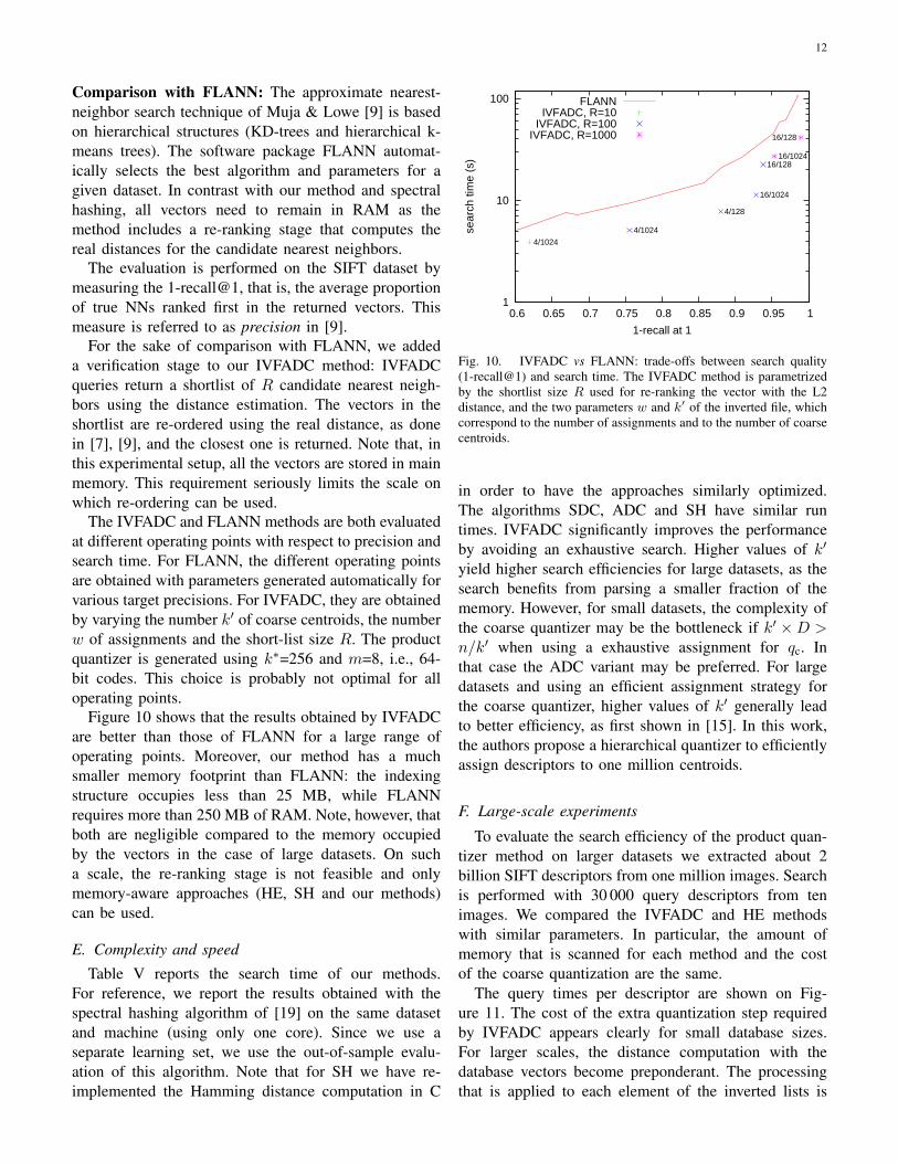
The IVFADC and FLANN methods are both evaluatedat different operating points with respect to precision andsearch time. For FLANN, the different operating pointsare obtained with parameters generated automatically forvarious target precisions. For IVFADC, they are obtainedby varying the number k′ of coarse centroids, the numberw of assignments and the short-list size R. The productquantizer is generated using k∗=256 and m=8, i.e., 64-bit codes. This choice is probably not optimal for alloperating points.

Figure 10 shows that the results obtained by IVFADCare better than those of FLANN for a large range ofoperating points. Moreover, our method has a muchsmaller memory footprint than FLANN: the indexingstructure occupies less than 25 MB, while FLANNrequires more than 250 MB of RAM. Note, however, thatboth are negligible compared to the memory occupiedby the vectors in the case of large datasets. On sucha scale, the re-ranking stage is not feasible and onlymemory-aware approaches (HE, SH and our methods)can be used.

E. Complexity and speed

Table V reports the search time of our methods.For reference, we report the results obtained with thespectral hashing algorithm of [19] on the same datasetand machine (using only one core). Since we use aseparate learning set, we use the out-of-sample evalu-ation of this algorithm. Note that for SH we have re-implemented the Hamming distance computation in C

1

10

100

0.6 0.65 0.7 0.75 0.8 0.85 0.9 0.95 1

sear

ch ti

me

(s)

1-recall at 1

FLANNIVFADC, R=10

IVFADC, R=100IVFADC, R=1000

4/1024

4/1024

4/128

16/1024

16/12816/1024

16/128

Fig. 10. IVFADC vs FLANN: trade-offs between search quality(1-recall@1) and search time. The IVFADC method is parametrizedby the shortlist size R used for re-ranking the vector with the L2distance, and the two parameters w and k′ of the inverted file, whichcorrespond to the number of assignments and to the number of coarsecentroids.

in order to have the approaches similarly optimized.The algorithms SDC, ADC and SH have similar runtimes. IVFADC significantly improves the performanceby avoiding an exhaustive search. Higher values of k′

yield higher search efficiencies for large datasets, as thesearch benefits from parsing a smaller fraction of thememory. However, for small datasets, the complexity ofthe coarse quantizer may be the bottleneck if k′ ×D >n/k′ when using a exhaustive assignment for qc. Inthat case the ADC variant may be preferred. For largedatasets and using an efficient assignment strategy forthe coarse quantizer, higher values of k′ generally leadto better efficiency, as first shown in [15]. In this work,the authors propose a hierarchical quantizer to efficientlyassign descriptors to one million centroids.

F. Large-scale experiments

To evaluate the search efficiency of the product quan-tizer method on larger datasets we extracted about 2billion SIFT descriptors from one million images. Searchis performed with 30 000 query descriptors from tenimages. We compared the IVFADC and HE methodswith similar parameters. In particular, the amount ofmemory that is scanned for each method and the costof the coarse quantization are the same.

The query times per descriptor are shown on Fig-ure 11. The cost of the extra quantization step requiredby IVFADC appears clearly for small database sizes.For larger scales, the distance computation with thedatabase vectors become preponderant. The processingthat is applied to each element of the inverted lists is

13

method parameters search average number of recall@100time (ms) code comparisons

SDC 16.8 1 000 991 0.446ADC 17.2 1 000 991 0.652IVFADC k′= 1 024, w=1 1.5 1 947 0.308

k′= 1 024, w=8 8.8 27 818 0.682k′= 1 024, w=64 65.9 101 158 0.744k′= 8 192, w=1 3.8 361 0.240k′= 8 192, w=8 10.2 2 709 0.516k′= 8 192, w=64 65.3 19 101 0.610

SH 22.7 1 000 991 0.132

TABLE VGIST DATASET (500 QUERIES): SEARCH TIMINGS FOR 64-BIT CODES AND DIFFERENT METHODS. WE HAVE USED m=8 AND k∗=256

FOR SDC, ADC AND IVFADC.

0

0.5

1

1.5

2

2.5

3

3.5

10M 100M 1G

sear

ch ti

me

(ms/

vect

or)

database size

HEIVFADC

Fig. 11. Search times for SIFT descriptors in datasets of increasingsizes, with two search methods. Both use the same 20 000-wordcodebook, w = 1, and 64-bit signatures.

approximately as expensive in both cases. For HE, itis a Hamming distance computation, implemented as 8table lookups. For IVFADC it is a distance computationthat is also performed by 8 table lookups. Interestingly,the floating point operations involved in IVFADC are notmuch more expensive than the simple binary operationsof HE.

G. Image search

We have evaluated our method within an image searchsystem based on local descriptors. For this evaluation, wecompare our method with the HE method of [20] on theINRIA Holidays dataset, using the pre-processed set ofdescriptors available online. The comparison is focusedon large scale indexing, i.e., we do not consider the im-pact of a post-verification step [23], [31] or geometrical

0.4

0.45

0.5

0.55

0.6

0.65

0.7

0.75

0.8

1k 10k 100k 1M

mA

P

database size (number of images)

IVF+HE 64 bitsIVFADC 64 bits (m=8)

IVF+HE 32 bitsIVFADC 32 bits (m=4)

Fig. 12. Comparison of IVFADC and the Hamming Embeddingmethod of [20]. mAP for the Holidays dataset as function of thenumber of distractor images (up to 1 million).

information [20].

Figure 12 shows the search performance in terms ofmean average precision as a function of the size ofthe dataset. We have used the same coarse quantizer(k′=20,000) and a single assignment strategy (w=1) forboth the approaches, and fixed k∗=256 for IVFADC. Fora given number of bits (32 or 64), we have selected thebest choice of the Hamming threshold for HE. Similarly,we have adjusted the number of nearest neighbors to beretrieved for IVFADC.

One can observe that the gain obtained by IVFADC issignificant. For example, for one million distractors, themAP of 0.497 reported in [20] with 64-bit signatures isimproved to 0.517.

14

VI. CONCLUSION

We have introduced product quantization for approx-imate nearest neighbor search. Our compact codingscheme provides an accurate approximation of the Eu-clidean distance. Moreover, it is combined with an in-verted file system to avoid exhaustive search, resulting inhigh efficiency. Our approach significantly outperformsthe state of the art in terms of the trade-off betweensearch quality and memory usage. Experimental resultsfor SIFT and GIST image descriptors are excellent andshow that grouping the components based on our priorknowledge of the descriptor design further improves theresults. The scalability of our approach is validated on adataset of two billion vectors.

REFERENCES

[1] H. Jegou, M. Douze, and C. Schmid, “Searching with quanti-zation: approximate nearest neighbor search using short codesand distance estimators,” Tech. Rep. RR-7020, INRIA, August2009.

[2] H. Sandhawalia and H. Jegou, “Searching with expectations,” inIEEE International Conference on Acoustics Speech and SignalProcessing, Signal Processing, pp. 1242–1245, IEEE, March2010.

[3] K. Beyer, J. Goldstein, R. Ramakrishnan, and U. Shaft, “Whenis ”nearest neighbor” meaningful?,” in Proceedings of theInternational Conference on Database Theory, pp. 217–235,August 1999.

[4] C. Bohm, S. Berchtold, and D. Keim, “Searching in high-dimensional spaces: Index structures for improving the per-formance of multimedia databases,” ACM Computing Surveys,vol. 33, pp. 322–373, October 2001.

[5] J. Friedman, J. L. Bentley, and R. A. Finkel, “An algorithmfor finding best matches in logarithmic expected time,” ACMTransaction on Mathematical Software, vol. 3, no. 3, pp. 209–226, 1977.

[6] R. Weber, H.-J. Schek, and S. Blott, “A quantitative analysisand performance study for similarity-search methods in high-dimensional spaces,” in Proceedings of the International Con-ference on Very Large DataBases, pp. 194–205, 1998.

[7] M. Datar, N. Immorlica, P. Indyk, and V. Mirrokni, “Locality-sensitive hashing scheme based on p-stable distributions,” inProceedings of the Symposium on Computational Geometry,pp. 253–262, 2004.

[8] A. Gionis, P. Indyk, and R. Motwani, “Similarity search in highdimension via hashing,” in Proceedings of the InternationalConference on Very Large DataBases, pp. 518–529, 1999.

[9] M. Muja and D. G. Lowe, “Fast approximate nearest neighborswith automatic algorithm configuration,” in Proceedings ofthe International Conference on Computer Vision Theory andApplications, 2009.

[10] B. Kulis and K. Grauman, “Kernelized locality-sensitive hash-ing for scalable image search,” in Proceedings of the Interna-tional Conference on Computer Vision, October 2009.

[11] G. Shakhnarovich, T. Darrell, and P. Indyk, Nearest-NeighborMethods in Learning and Vision: Theory and Practice, ch. 3.MIT Press, March 2006.

[12] Y. Ke, R. Sukthankar, and L. Huston, “Efficient near-duplicatedetection and sub-image retrieval,” in ACM International con-ference on Multimedia, pp. 869–876, 2004.

[13] B. Matei, Y. Shan, H. Sawhney, Y. Tan, R. Kumar, D. Huber,and M. Hebert, “Rapid object indexing using locality sensitivehashing and joint 3D-signature space estimation,” IEEE Trans-actions on Pattern Analysis and Machine Intelligence, vol. 28,pp. 1111 – 1126, July 2006.

[14] C. Silpa-Anan and R. Hartley, “Optimized kd-trees for fastimage descriptor matching,” in Proceedings of the IEEE Con-ference on Computer Vision and Pattern Recognition, 2008.

[15] D. Nister and H. Stewenius, “Scalable recognition with a vocab-ulary tree,” in Proceedings of the IEEE Conference on ComputerVision and Pattern Recognition, pp. 2161–2168, 2006.

[16] A. Torralba, R. Fergus, and W. T. Freeman, “80 million tinyimages: a large database for non-parametric object and scenerecognition,” IEEE Transactions on Pattern Analysis and Ma-chine Intelligence, vol. 30, pp. 1958–1970, November 2008.

[17] A. Torralba, R. Fergus, and Y. Weiss, “Small codes and largedatabases for recognition,” in Proceedings of the IEEE Confer-ence on Computer Vision and Pattern Recognition, 2008.

[18] A. Oliva and A. Torralba, “Modeling the shape of the scene:a holistic representation of the spatial envelope,” InternationalJournal of Computer Vision, vol. 42, no. 3, pp. 145–175, 2001.

[19] Y. Weiss, A. Torralba, and R. Fergus, “Spectral hashing,” inAdvances in Neural Information Processing Systems, 2008.

[20] H. Jegou, M. Douze, and C. Schmid, “Hamming embedding andweak geometric consistency for large scale image search,” inProceedings of the European Conference on Computer Vision,October 2008.

[21] M. Douze, H. Jegou, H. Singh, L. Amsaleg, and C. Schmid,“Evaluation of GIST descriptors for web-scale image search,”in Proceedings of the International Conference on Image andVideo Retrieval, 2009.

[22] J. Philbin, O. Chum, M. Isard, J. Sivic, and A. Zisserman, “Lostin quantization: Improving particular object retrieval in largescale image databases,” in Proceedings of the IEEE Conferenceon Computer Vision and Pattern Recognition, 2008.

[23] D. Lowe, “Distinctive image features from scale-invariant key-points,” International Journal of Computer Vision, vol. 60,no. 2, pp. 91–110, 2004.

[24] R. M. Gray and D. L. Neuhoff, “Quantization,” IEEE Trans-actions on Information Theory, vol. 44, pp. 2325–2384, Oct.1998.

[25] D. E. Knuth, The Art of Computer Programming, Sorting andSearching, vol. 3. Addison Wesley, 2 ed., 1998.

[26] J. Sivic and A. Zisserman, “Video Google: A text retrievalapproach to object matching in videos,” in Proceedings of theInternational Conference on Computer Vision, pp. 1470–1477,2003.

[27] M. Perdoch, O. Chum, and J. Matas, “Efficient representation oflocal geometry for large scale object retrieval,” in Proceedingsof the IEEE Conference on Computer Vision and PatternRecognition, June 2009.

[28] H. Jegou, M. Douze, and C. Schmid, “Packing bag-of-features,”in Proceedings of the International Conference on ComputerVision, September 2009.

[29] H. Jegou, H. Harzallah, and C. Schmid, “A contextual dis-similarity measure for accurate and efficient image search,” inProceedings of the IEEE Conference on Computer Vision andPattern Recognition, 2007.

[30] H. Cho, I. Dhillon, Y. Guan, and S. Sra, “Minimum sum-squared residue co-clustering of gene expression data,” in SIAMInternational Conference on Data Mining, pp. 114–125, April2004.

[31] J. Philbin, O. Chum, M. Isard, J. Sivic, and A. Zisserman, “Ob-ject retrieval with large vocabularies and fast spatial matching,”in Proceedings of the IEEE Conference on Computer Vision andPattern Recognition, 2007.