Journal of Software Engineering for Robotics 3(1), March 2012, 2-12ISSN: 2035-3928

Comparison of nearest-neighbor-search strategies

and implementations for efficient shape registrationJan Elseberg1,∗ Stephane Magnenat2 Roland Siegwart2 Andreas Nuchter1

1 Automation Group, Jacobs University Bremen gGmbH, 28759 Bremen, Germany2 Autonomous Systems Lab, ETH Zurich, Switzerland ∗jan.elseberg@jacobs-university.de

Abstract—The iterative closest point (ICP) algorithm is one of the most popular approaches to shape registration currently in use. At

the core of ICP is the computationally-intensive determination of nearest neighbors (NN). As of now there has been no comprehensive

analysis of competing search strategies for NN. This paper compares several libraries for nearest-neighbor search (NNS) on both

simulated and real data with a focus on shape registration. In addition, we present a novel efficient implementation of NNS via k-d trees

as well as a novel algorithm for NNS in octrees.

Index Terms—shape registration, nearest neighbor search, k-d tree, octree, data structures

1 INTRODUCTION

Shape registration is the problem of finding the rigid trans-

formation that, given two shapes, transforms one onto the

other. The given shapes do not need to be wholly identical.

As long as a partial overlap is possible, shape registration

seeks the transformation that accomplishes just that overlap.

For the extent of this paper we consider a shape to be a set of

points in three-dimensional Cartesian space, i.e. a point cloud.

The registration problem is most commonly solved using the

iterative closest point (ICP) algorithm [1]. In addition to the

two shapes, it assumes an estimate of the transformation to be

computed. Such an estimate is usually available in contexts

where shape matching is of importance. ICP is an iterative

algorithm that alternates between determining, based on the

current transformation estimate, the nearest neighbors (NN) of

every point of one shape, and updating the estimate based on the

NN. Updating the estimate is a relatively simple mathematical

operation that is linear in the number of neighboring points.

Naively implemented, the nearest-neighbor search (NNS) is

in O(nm) where n and m are the number of points in the

respective point clouds. Exploring every possible pairing of

Regular paper – Manuscript received October 21, 2011; revised February

15, 2012.

• This work was partially supported by the AUTOSCAN project (BMWi

KF2470003DF0).

• Authors retain copyright to their papers and grant JOSER unlimited

rights to publish the paper electronically and in hard copy. Use of the

article is permitted as long as the author(s) and the journal are properly

acknowledged.

point can be avoided by employing spatial data structures.

The average runtime of NNS is then usually in the order

of O(n logm) but is still by far the most computationally

expensive part of shape registration. This paper gives a

comprehensive empirical analysis of NNS algorithms in the

domain of 3-dimensional shape matching. For this purpose,

section 2 gives an overview of spatial data structures and the

state of the art on comparison of search algorithms. Section 3

presents the novel search algorithm on octrees and the novel

efficient implementation of NNS in k-d trees. We explain our

experimental setup in section 4, provide results in section 5

and conclude the paper in section 6.

2 RELATED WORK

Spatial data structures partition space to allow efficient access

to the stored elements via positional queries. Most spatial data

structures are hierarchical in nature, such as k-d trees [9] and

octrees [10]. The grid file [11] is a rare flat non-hierarchical

data structure. We explicitly exclude it from consideration here

because of its prohibitive memory requirements. A special type

of NNS employs the Morton order for arranging the point cloud.

A Morton order is a space-filling curve (SFC), i.e. a curve that

allows ordering the set of points along one dimension while

preserving the locality thereof [12].

In addition to the well known k-d tree and octree we also

consider the following hierarchical R-trees [13]. There are other

data structures such as the range-tree [14] and vp-tree [15].

Unfortunately, to the authors’ knowledge, there is no publicly

available NNS library that employs either the vp- or the range-

tree.

www.joser.org - © 2012 by Jan Elseberg, Stephane Magnenat, Roland Siegwart, Andreas Nuchter

J. Elseberg et al./ Comparison of nearest-neighbor-search strategies and implementations for efficient shape registration 3

TABLE 1

Properties for all tested NNS libraries.

Library revisionData k-NN fixed ranged

optimized forstructure search radius search

3DTK [2] rev. 470 k-d tree × × X shape registration3DTK rev. 470 octree × × X shape registration & efficient storage

ANN [3] Ver. 1.1.1 k-d tree X X ×CGAL [4] Ver. 3.5.1-1 k-d tree × X ×

FLANN [5] bcf3a56e5fed2d4dc3a340725fa341fa36ef79a4 k-d tree X X × high dimensionslibnabo [6] Ver. 1.0.0 k-d tree X × X

SpatialIndex [7] Ver. 1.4.0-1.1 R-tree X × ×STANN [8] Ver. 0.71 beta SFC X × × multithreading

An octree [10] is the generalization of quadtrees, which store

two dimensional data [16]. Each node in an octree represents

the volume formed by a rectangular cuboid, often simplified

to an axis-aligned cube. Consequently an octree node has

up to eight children, each corresponding to one octant of the

overlying cube/node. A node having no children usually implies

that the corresponding volume can be uniformly represented,

i.e., no further subdivision is necessary to disambiguate. This

convention is not completely applicable when storing points,

which are dimensionless, i.e., there is no volume associated

with them. When storing a point cloud, a stopping rule must

be defined for occupied volumes, like a maximal depth or a

minimal number of points. Empty volumes will however not

be further split up.

The k-d tree [9] is similar to the octree in that each node

represents an axis-aligned rectangular cuboid and its children

split up the volume to form smaller cuboids. Empty volumes

are not subdivided further, and there must be a stopping rule

for occupied volumes. However, a k-d tree is a binary tree and

the subdivision of the node’s volume must not be regular, i.e.

each node also defines an axis-aligned hyperplane that splits

the volume in two. Unlike the octree, there is not a unique

way of constructing a k-d tree since the splitting plane can be

placed at any position in any node. There are several strategies

for placing the splitting plane. The standard rule is splitting

before the median point along the longest dimension of the

node’s volume. Another splitting rule is the so called midpoint

rule, which merely splits the current volume in half along its

longest dimension.

The R-tree [13] is non-binary and is primarily used for spatial

data other than point clouds, i.e. for geographic information

systems. Each node represents an axis-aligned bounding box

of arbitrary dimension. The represented volumes are allowed

to overlap, except for the requirement that a child’s volume

must be entirely within the parent’s. There are several variants

of the R-tree that differ only in their insertion algorithms.

The linear, quadratic and exponential R-tree all insert a new

element into the node that requires the least extension, but

they use algorithms of different complexities (hence the name)

for splitting the node, if necessary. The R*-tree insertion

algorithm chooses which node to insert the new element into

by a minimum overlap criteria. It also extends the splitting

algorithm by the principle of forced reinsertion, i.e. elements

that are already stored may be deleted and reinserted into

another node [17].

Apart from the data structure, the NNS queries are of interest.

There are different types of NNS query that deserve discussion:

The first type of query that springs to mind in the context

of NNS is the k-NN search. The result of this type of query

are the k NN around a specified query point. Another is the

fixed radius search, which computes all points withing a given

radius of the query point. The combination of the two types

yields the ranged search, i.e. the retrieval of the k NN with

a given maximal distance. The latter query with k = 1 is

the type of query needed for shape registration. In the large

majority of realistic applications the presence of obstruction

leads to only partially-overlapping point clouds. Thus, allowing

point correspondences with a too large distance can only infuse

the registration process with errors. The range search variant

also allows for a large potential for efficient implementation.

The maximal radius restricts the search region to only a small

subspace of the entire data. This can be efficiently combined

with the restriction on the number of points. Even the small

subspace does not need to be explored in its entirety if it can be

ensured that the k NN points have been located. It is surprising

then, that many NNS libraries fail to provide this search variant

(cf. Table 1).

To the authors’ knowledge there is little previous work

exploring and comparing current NNS libraries in the context of

shape registration. Blumenthal et al. [18] give a first evaluation

of some available NNS libraries. We compare a wider range of

algorithms on a wider range of data, both artificial and real.

Pomerleau at al. [19] explore several parameters influencing

registration performance, but only one parameter (an early-out

approximation factor) is related to the NNS. There have been

comparisons of different data structures for NNS, although

not specifically for shape registration. Dandamudi et al. [20]

compare the binary decision (bd) tree to variants of the k-d

tree. Nakamura et al. [21] propose a new data structure, the

md-tree and compare it against the k-d tree and the bd-tree.

They also find the k-d tree to perform worse than the other data

structures in the tested scenarios. Judging from the large number

4 Journal of Software Engineering for Robotics 3(1), March 2012

of libraries employing the k-d tree it is clear that it is still

the favored data structure in general NNS libraries. Greenspan

et al. [22], [23] have proposed improved NNS algorithms for

shape registration. While these are promising, they have not

yet found their way into any of the NN libraries evaluated in

this paper.

3 DESIGN AND IMPLEMENTATION

In this section we present our highly-optimized implementation

of the octree and k-d tree. The octree implementation has

specifically been designed for the efficient storage of large

point clouds. It is implemented in the 3DTK [2] and supports

NNS, point-cloud compression and fast visualization. The fast

k-d tree implementation is called libnabo [6] and is not to

be confused with the simple k-d tree implementation within

3DTK.

3.1 Octree

Our octree code implements a novel search algorithm as

presented in this section. It is written in ISO/IEC C++ 2003

and is integrated into the 3DTK framework as a visualization,

shape detection and NNS data structure. It does not rely on

other libraries to store its nodes and geometry data as it is

optimized for memory efficiency [24]. It is templated to allow

for choosing the precision of the point data.

Principally, octrees should allow for extremely efficient

implementations of NNS. Due to their regular partitioning of

the search space and the high branching factor, coordinate

queries are very fast [25]. Yet, most NN libraries are based on

k-d trees.

The complication is due to the fact that during NNS, nodes

near the query point must be visited. Thus an order of traversal

must be found that is both efficient, in that it visits no more

nodes than necessary, and easy to compute. The key to an

efficient traversal is the order in which children are visited.

The number of nodes that need to be visited is best reduced

by the closest-child first criteria, i.e. the order of traversal is

determined by the distance to the query point. This is trivial

to do for the binary k-d tree, but more involved for an octree.

For any node with 8 children there are a total of 96 possible

sequences in which to traverse the children. A query point

may fall into or be closest to any one of the 8 octants. This is

the first child to traverse. For each of those cases there are 12possibilities in which to traverse further. This is determined

by the proximity of the query point to the 3 split planes. The

next two children to visit are, in order, the two closest of the

three direct neighbors of the first child. The fourth child to

visit is either the last remaining direct neighbor or the node

that complements the cuboid of visited nodes. The sequence in

which to visit the remaining four nodes is entirely dependent

on the traversal before and can not change. Thus, there are

8 · 3 · 2 · 2 = 96 possible traversals in whole.

Algorithm 1 FindClosest

Input: query point q, maximal allowed distance dlookup deepest node N containing bounding box of qconvert q to octree coordinate ireturn FindClosestInNode(N , q, i, d)

Algorithm 2 FindClosestInNode

Input: query point q and its coordinate iInput: maximal allowed distance d and the current node N

1: compute child index c from i2: for j = 0 to 7 do3: get next closest child C = N .children[sequence[c][j]]4: if C is outside of bounding ball then5: return currently closest point p6: else7: if C is a leaf then8: FindClosestInLeaf(C, q, d)9: update currently closest point p

10: else11: FindClosestInNode(C, q, i, d)12: update currently closest point p13: end if14: end if15: end for16: return currently closest point p

NNS in an octree has to make proximity calculations to

3 split planes, sort the distances and select the appropriate

sequence of traversal for every traversed node. Compared to

this, the order of traversal in a k-d tree is instantly determined

by a single proximity check, thereby avoiding unnecessary

computations if nodes need not be visited.

However, the regular subdivisions of an octree can still be

leveraged for fast NNS. The biggest benefit is that fast indexing

is possible in an octree. This allows us to directly traverse to

the deepest octree node, which contains the bounding sphere

of the query point. This is done with a constant number of

floating-point operations and is considerably faster than the

equivalent operation in a k-d tree, which is essentially a lookup

of a point already in the tree. However, the speedup gained

is clearly dependent on the maximal distance allowed to the

query point. The smaller this distance is, the deeper the node

enclosing the bounding sphere is on average. The closest child

first NNS with backtracking is then performed on this node,

i.e. the deeper the node, the fewer the number of steps needed

in the NNS.

The number of floating-point operations needed to choose

the correct order of traversal out of the 96 possibilities at each

node is exceedingly high. By restricting ourselves to 8 possible

traversals it is possible to eliminate the need for any floating

point operations in the inner nodes. The order of traversal is

decided by which octant the query point is closest to. This is

done in accordance to Frisken and Perry [25] and requires no

floating-point operations. Each of the 8 traversals are identical

in nature, first the closest octant is visited, then the three

direct neighbors, then the three direct neighbors of those and

J. Elseberg et al./ Comparison of nearest-neighbor-search strategies and implementations for efficient shape registration 5

finally the most distant node. The approach is summarized

in Algorithm 1. The function FindClosestInLeaf is the

NNS inside a leaf, a floating-point proximity check of all stored

points.

3.2 k-d tree

Our fast k-d tree implementation is called libnabo [6]. Its tree

creation and search algorithm is similar to ANN [26], a well-

established library [3], but it differs in the implementation de-

tails, which significantly improves performance (see Section 5).

libnabo is written in ISO/IEC C++ 2003 and provides a nearest-

neighbor–search interface, allowing to easily add new search

strategies through inheritance. The current version of libnabo

provides a brute-force strategy for comparison purpose and

the kd-tree strategy. Geometry data are stored in Eigen 3 [27]

structures, as this library is quickly becoming a standard for

linear algebra in robotics research1. Other data such as the

neighbors heap and the tree nodes are stored in STL containers,

such as std::vector.

For creating the tree, libnabo uses the sliding-midpoint rule,

that is, when considering a cuboid, it tries to cut it by the

middle on its dimension of maximal extent. If this results

in a trivial split, that is, if there is one side with no points,

libnabo moves the splitting plane such that there is at least

one point on each side. The search algorithm is also similar

to ANN, doing a recursive descent on the side of the cutting

plane the closest to the search point; and exploring alternative

branches while going back up until the k NN are closer than the

cutting planes. Algorithm 3 gives an overview of this method.

Initially, the minimum distances D to other points for every

dimension and their norm r are 0. The heap H of size k holds

the current candidates for the k NN and allows fast check and

insertion. libnabo provides two implementations, a linear- and

a tree-based heap. The linear heap is suitable for small k, as

it has a complexity of O(k) with a small constant while the

tree heap is in O(log k) but with a larger constant. We have

experimentally found that up to k = 30, the linear version is

faster. Note that D and H are passed as mutable references.

The other parameters are either passed as constant references

or as mutable values.

The difference with ANN lies at the level of data structures.

Where ANN employs a tree of objects based on pointers,

libnabo uses a compact vector of nodes. To understand why

this difference is significant, let us consider floating-point data

on a 64-bit architecture and compute the memory footprint.

For every split node, ANN holds the cutting dimension (4

bytes), the cutting value (4 bytes), the lower and the upper

bounds (8 bytes), and pointers to left and right children (16

bytes). Moreover, the node being a virtual object, it holds

at least a pointer to its vtable (8 bytes). Therefore, a single

node consumes at least 40 bytes of memory. On the contrary,

1. it is being used by ROS and MRPT for instance

Algorithm 3 LibnaboFindClosest

Input: query point q, node N , heap H , minimum distance r,Input: minimum offsets D, maximal squared allowed distance l

if N is a leaf node thensearch for closest points to q in bucket pointed by Nupdate H

elseget cut dimension c and cut value v from Noold = D[c], onew = q[c]− vif onew > 0 then

LibnaboFindClosest(q, rightChild(N ), H , r, D, l)r = r − o2old + o2new

if r ≤ l and r < head(H) thenD[c] = onew

LibnaboFindClosest(q, leftChild(N ), H , r, D, l)D[c] = oold

end ifelse

LibnaboFindClosest(q, leftChild(N ), H , r, D, l)r = r − o2old + o2new

if r ≤ l and r < head(H) thenD[c] = onew

LibnaboFindClosest(q, rightChild(N ), H , r, D, l)D[c] = oold

end ifend if

end if

libnabo’s node is a non-virtual class2 that contains only the

cutting dimension and index of right child (first 4-bytes word),

and a union of the cutting value or the bucket index (second

4-bytes word). Indeed, if the cutting dimension (the least-

significant bits of the first word) is smaller than the number

of dimensions, the node is a split node and the second word

contains the cutting value. In this case, the left child is the

index of this node plus one, and the right child is encoded in

the most-significant bits of the first word. On the contrary, if

the cutting dimension is equal to the number of dimensions,

this node is a leaf node and the second word contains the

index of the bucket. This index points to a dense array of point

indices, allowing the search algorithm to access the points.

Therefore, a node in libnabo is only 8 bytes, a 5-fold spare in

memory compared to ANN.

4 EXPERIMENTAL METHODOLOGY

Many factors influence the performance of a NNS query. One

factor is the maximal distance parameter, which restricts

the search space around the query point. The larger the

maximal distance the more of the space the search routine

must explore. A second factor is the type of data on which

the NN query is being performed. Some data may result in

optimally constructed data structures, while others may lead

to unfavorable configurations. For this reason we carry out

2. Note that the node class is a private inner class in a subclass of thenearest-neighbor–search interface. This interface is implemented as a superclasswith virtual members and a static factory function. Thus libnabo is extensiblethrough inheritance.

6 Journal of Software Engineering for Robotics 3(1), March 2012

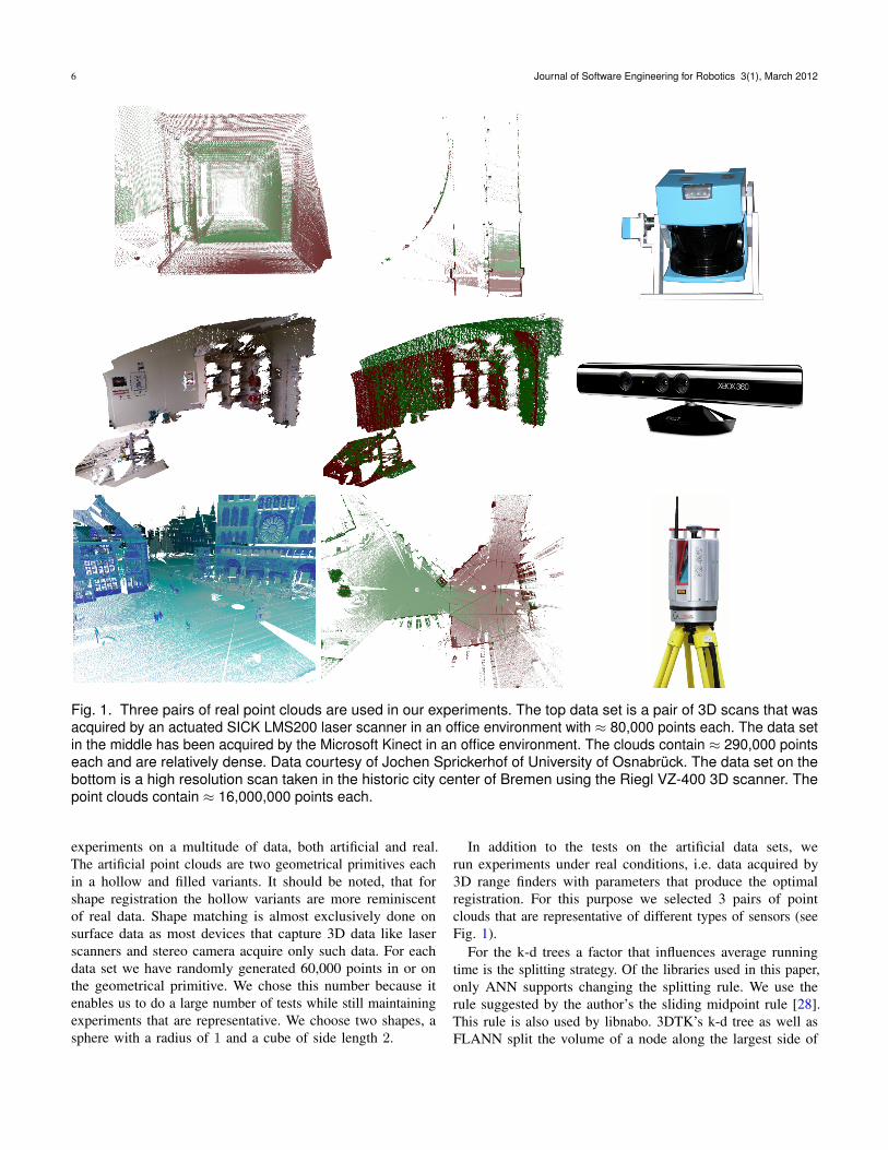
Fig. 1. Three pairs of real point clouds are used in our experiments. The top data set is a pair of 3D scans that was

acquired by an actuated SICK LMS200 laser scanner in an office environment with ≈ 80,000 points each. The data set

in the middle has been acquired by the Microsoft Kinect in an office environment. The clouds contain ≈ 290,000 points

each and are relatively dense. Data courtesy of Jochen Sprickerhof of University of Osnabruck. The data set on the

bottom is a high resolution scan taken in the historic city center of Bremen using the Riegl VZ-400 3D scanner. The

point clouds contain ≈ 16,000,000 points each.

experiments on a multitude of data, both artificial and real.

The artificial point clouds are two geometrical primitives each

in a hollow and filled variants. It should be noted, that for

shape registration the hollow variants are more reminiscent

of real data. Shape matching is almost exclusively done on

surface data as most devices that capture 3D data like laser

scanners and stereo camera acquire only such data. For each

data set we have randomly generated 60,000 points in or on

the geometrical primitive. We chose this number because it

enables us to do a large number of tests while still maintaining

experiments that are representative. We choose two shapes, a

sphere with a radius of 1 and a cube of side length 2.

In addition to the tests on the artificial data sets, we

run experiments under real conditions, i.e. data acquired by

3D range finders with parameters that produce the optimal

registration. For this purpose we selected 3 pairs of point

clouds that are representative of different types of sensors (see

Fig. 1).

For the k-d trees a factor that influences average running

time is the splitting strategy. Of the libraries used in this paper,

only ANN supports changing the splitting rule. We use the

rule suggested by the author’s the sliding midpoint rule [28].

This rule is also used by libnabo. 3DTK’s k-d tree as well as

FLANN split the volume of a node along the largest side of

J. Elseberg et al./ Comparison of nearest-neighbor-search strategies and implementations for efficient shape registration 7

Fig. 2. ICP runtime in seconds on the SICK LMS200 data

set.

the bounding box of the contained points. CGAL employs the

standard median splitting rule along an axis dependent on the

level of the tree.

Another notable parameter is the minimal number of points

per leaf in the data structure, i.e. the bucket size. The smaller

the bucket size is the larger is the overhead of the additional

levels in the tree. The larger the bucket size the more points will

have to be searched in a linear fashion. An evaluation on the

SICK LMS200 data set (cf. Fig. 2), reveals that a bucket size

between 5 and 20 is usually optimal. However, these results

are not entirely representative and depend on the data sets used.

In our experiments on artificial data, where trends are observed

rather than absolute comparisons to be made, we use the default

bucket size of the respective libraries, with two exceptions. In

both FLANN and SpatialIndex we set the bucket size to be

10. This is also the default for most other libraries. In FLANN

there is no default bucket size, so a choice had to be made. For

SpatialIndex the default is 100 because it is intended that the

data structure is cached to disk. However we run SpatialIndex

in main memory and a bucket size of 100 gives significantly

worse performance. For the experiments under real conditions

the absolute running time instead of the trends in the runtime

is the most important criteria. To provide clear results we set

the bucket sizes to the optimal size as derived from Fig. 2,

i.e. 5 for libnabo and 15 for both 3DTK data structures and

FLANN. ANN does not allow for the changing of the bucket

size.

Approximate search algorithms for the k-d tree, i.e. NNS with

no guarantee of finding the exact NN, exist [29] but we opt to

only test the exact NNS, since only this is implemented by all

libraries. We use two variants of the R-tree for our experiments,

the quadratic R-tree and the R*-tree. The exponential R-tree is

not implemented in SpatialIndex, and the quadratic variant

outperforms the linear one in all our experiments. Three

libraries, ANN, FLANN and libnabo support more than a

single NN query. Since ANN and FLANN do not support the

ranged search, both queries are tested for both libraries. For

Fig. 3. The runtimes from all algorithms for the hollow

cube/sphere combination. The query point set is the cube,

whereas the sphere is the model data set. Left: Runtimes

are plotted on a logarithmic scale to give an overview.

Right: Runtimes are plotted on a linear scale in a smaller

subsection.

libnabo, only the ranged search is tested as the k-NN search is

implemented as a special case of the ranged search.

We compare a large set of NNS libraries: 3DTK, ANN,

CGAL, FLANN, libnabo, SpatialIndex and STANN. Most of

these rely on the k-d tree, in fact of these 3DTK is the only

library implementing the octree, SpatialIndex the only one to

rely on R-trees and STANN is the only one using SFCs. Only

very few libraries feature multithreading capabilities, therefore

all experiments were performed in single-threaded mode. The

results of every library on a handful of chosen testcases has

been compared to each other to confirm their correctness.

8 Journal of Software Engineering for Robotics 3(1), March 2012

Fig. 4. The average times needed for creating different

data structures. Note, that due to the large differences

in the times the y-axis has been split into a linear and

logarithmic scale.

All libraries were compiled with the gnu compiler collection

version 4.4.3 on optimization level 3. The system running all

experiments is a 64 Bit Xubuntu Linux (kernel 2.6.32-27) with

an Intel(R) Xeon(R) E5520@2.27GHz and 12 GB of memory.

5 RESULTS

The most extensive experiments were done on the aforemen-

tioned artificial data sets. For each library we varied the

maximal range allowed for the NN from 0 to 1 in steps of 0.02.

We repeated the NNS in 100 trials, and plotted the averaged

running time.

An interesting combinations of query and model data set is

presented in Fig. 3. It is a combination that resembles shape

matching most closely, as both the query data set (the cube)

and the model data set (the sphere) are surfaces. Clearly, the

runtime of the ranged and fixed radius search depend strongly

on the maximal distance. The larger the allowed distance, the

more query points (near the cube’s corners) have a NN. The

more NN that need to be found, and the farther away these

are, the longer the search will need to finish. Larger distances

affect the fixed radius search algorithms significantly more than

the ranged searches. The runtime for the fixed radius search

continues to rise polynomially, whereas the ranged searches

level off near√

(3) ≈ 0.73, which is the maximum possible

distance in the data set. The runtime of the k-NN search is of

course not influenced by the maximal distance. Most of them

are significantly slower than the ranged searches.

Due to the polynomial behavior of the runtime of the fixed

radius algorithms all of the k-NN are faster for large enough

maximal distances. However, only the ANN and FLANN library

perform similar or better than the ranged searches for large

enough maximal distances. Similar behavior is exhibited in

other combinations. For an overview see Fig. 6. Note, that

due to the large differences in running time, the time is on a

logarithmic scale. For plots on a linear scale see Fig. 7.

There is a large discrepancy in the running time for the

search libraries. This discrepancy falls quite neatly along

the lines of which type of algorithm is implemented. In

almost all cases the best performing NN libraries were those

implementing the ranged search, i.e. 3DTK and libnabo. The

libraries only implementing k-NN search, i.e. STANN, CGAL

and SpatialIndex can not compete with other algorithms. The

remaining libraries, ANN and FLANN are in a few cases faster

than some ranged search implementations. For a clearer look

into this region, please see Fig. 7. In all non-trivial cases, i.e.

when the query data set and the model data set are distinct,

libnabo is faster than both FLANN and ANN. There are

2 exceptions to this, where libnabo is equal in runtime to

FLANN and ANN. This occurs when the maximal range is

at significant fractions of the point clouds size, i.e. ≈ 1

3to

1

2. This is also the range at which FLANN and ANN start to

beat the other ranged search algorithms. Before this the ranged

search implementations are faster than both the k-NN search

implementations and the fixed radius search implementations.

For shape matching the region of smaller maximal distances

are crucial. During the matching process the point clouds move

closer towards each other. The average point to point distance

is inherently reduced. The effect this has on the runtime of

the NNS can be tracked on the rightmost column in Fig. 6

and Fig. 7. On the top, the query points (hollow cube) are

farthest away from the model data set. The points are closer

with the filled cube, even closer with the hollow sphere and

finally identical with the filled sphere. The ranged searches as

well as the k-NN searches speed up due to this progression,

whereas the fixed radius search actually slow down.

However, absolute comparisons of the runtime may not be

valid based on these results alone when the runtime difference

is only several hundreds of milliseconds. Differences may be

caused by non-optimal bucket sizes (cf. 4) or by the artificial

nature of the data sets. In addition to the artificial data sets,

we therefore also compare the runtime of the 5 top performing

libraries on real data sets. To ensure bucket sizes play no role

in these results, we have chosen the optimal values as per

Fig. 2. The results are presented in Fig. 5.

The previous trend of the ranged search libraries performing

better than FLANN and ANN continues. For the smaller data

sets the k-NN search performs with similar speeds as the ranged

search. For the large data set acquired by professional hardware,

the performance is significantly worse. The fixed radius search

can compete with the ranged search in the latter case but

is significantly worse in the smaller data sets. In contrast to

the experiments with artificial data, libnabo tends to perform

slightly worse than the 3DTK algorithms on real data sets. This

is likely due to the added overhead of converting the query

data set into data usable by libnabo, i.e. the 3DTK NNS has a

home field advantage.

J. Elseberg et al./ Comparison of nearest-neighbor-search strategies and implementations for efficient shape registration 9

Fig. 5. The results from the 5 top performing libraries for the real data sets. Data structure construction time is not

included in the figures.

All previous experiments were concerned with the runtime

of the NNS and excluded the time needed to construct the

data sets. Fig. 4 shows the average time for construction for

all data structures and every point cloud used in the previous

experiments as a model data set. On the whole the libraries

perform similarly, except for STANN and SpatialIndex, the

latter of which is especially slow. Compared to the time needed

for the NNS (Fig. 7) and the ICP (Fig. 5) the construction time is

usually negligible, especially considering that the data structure

needs to be constructed only once for the entire registration

process.

We see that libnabo is always faster than ANN, sometimes

by a small amount, often by at least a factor of two, and

sometimes much more. As both libraries implement the same

algorithm, this discrepancy is solely due to the compactness

of libnabo’s data structures, that consume at least 5 times

less memory than ANN’s. This is important, because modern

computer architectures have multiple levels of cache, and thus

memory access is often the bottleneck [30]. The compactness

provided by libnabo comes at the price of additional and

repeated computations during the exploration of the tree. Yet

these work on local variables that are easily contained in cache

level 1. This shows that the NNS problem is clearly memory-

bound in general and that the choice of compactness is sound.

6 CONCLUSION

We have made a significant finding regarding the type of search

algorithm to use for shape registration. Ranged search queries

are ideally suited for shape matching and beat the alternatives in

all relevant cases. The reason for this is that shape registration

purposefully minimizes the distance to the NN. In the beginning

of the registration process the NN range is at its largest. Most

ICP iterations are done when the NN range is very small. In

fact, the maximal range to begin with is usually only a small

fraction of the point clouds’ extent. For our artificial data sets a

maximal range of ≈ 1

2constitutes the largest reasonable range

for shape matching.

There is yet another complication for the fastest alternatives

to ranged search, i.e. FLANN and ANN in these regions.

Choosing between the k-NN and the fixed search is non-trivial.

This would involve guessing which of the two is more efficient

for a given data set and a given maximal range. Since the

runtime of the fixed radius search explodes for large ranges, a

shape registration library would have to default to k-NN search.

The performance of k-NN search is reasonable on average, but

bad in just the region that is important for shape matching.

Since most libraries implement only the k-d tree, it is hard to

draw final conclusions as to what data structure is better suited

for NNS. The R-tree library SpatialIndex performs about on par

to the STANN library. Both were generally slower than the k-d

tree implementations. The octree implementation was amongst

the best performing algorithms. This effect may not be due

to the data structures alone. As Table 1 shows, SpatialIndex

was optimized for GIS systems, STANN for multithreaded

application while the octree implementation was designed to

be used in shape matching.

We have contributed our own novel open-source implementa-

tion of NNS and have shown these to perform well on realistic

as well as artificial shape registration problems. We have shown

that for similar algorithms, the compactness of data structures

plays a critical role and carefully-designed structures can double

performances.

SUPPLEMENTAL MATERIAL

We provide the code as well as the data used to perform

all experiments in this paper. Everything is available as a

subversion repository under http://slam6d.svn.sourceforge.net/

viewvc/slam6d/branches/NNS/. The implemented search algo-

rithms are freely available under http://slam6d.sourceforge.net/

and https://github.com/ethz-asl/libnabo.

ACKNOWLEDGMENTS

The authors would like to thank Dorit Borrmann for her support

in the data analysis.

10 Journal of Software Engineering for Robotics 3(1), March 2012

Fig. 6. The results from all algorithms for the artificial data sets on a logarithmic scale. The images on the x-axis

indicate the data set that was stored in the data structure (model set). The images on the y-axis indicate the query

point set. The query time in seconds required for the entire data set is plotted on a logarithmic scale for all settings of

the maximal allowed distance. The maximal distance was altered between 0 and 1 in steps of 0.02. Construction time

for the data structures is not included.

J. Elseberg et al./ Comparison of nearest-neighbor-search strategies and implementations for efficient shape registration 11

Fig. 7. The results from the best performing algorithms for the artificial data sets on linear scale. Note that the scale

has also been changed from 0 to 1 s.

12 Journal of Software Engineering for Robotics 3(1), March 2012

REFERENCES

[1] P. Besl and N. McKay, “A Method for Registration of 3–D Shapes,”IEEE Trans. PAMI, vol. 14, no. 2, pp. 239 – 256, February 1992. 1

[2] Automation Group (Jacobs University Bremen) and Knowledge-BasedSystems Group (University of Osnabruck), “3DTK – The 3D Toolkit,”http://slam6d.sourceforge.net/, February 2011. 1, 3

[3] D. M. Mount and S. Arya, “ANN: A Library for Approximate NearestNeighbor Searching,” http://www.cs.umd.edu/∼mount/ANN/, October2011. 1, 3.2

[4] “CGAL, Computational Geometry Algorithms Library,” http://www.cgal.org. 1

[5] M. Muja, “FLANN - fast Library for Approximate Nearest Neighbors,”http://people.cs.ubc.ca/∼mariusm/index.php/FLANN/FLANN, October2011. 1

[6] S. Magnenat, “libnabo,” https://github.com/ethz-asl/libnabo, October2011. 1, 3, 3.2

[7] M. Hadjieleftheriou, “SpatialIndex,” http://libspatialindex.github.com/,October 2011. 1

[8] M. Connor, “STANN - The simple, Thread-safe Approximate Near-est Neighbor Library,” http://sites.google.com/a/compgeom.com/stann/,October 2011. 1

[9] J. L. Bentley, “Multidimensional Binary Search Trees Used for Associa-tive Searching,” Comms. of the ACM, vol. 18, no. 9, pp. 509–517, 1975.2

[10] D. Meagher, “Geometric modeling using octree encoding,” Computer

Graphics and Image Processing, vol. 19, no. 2, pp. 129 – 147, 1982. 2[11] J. Nievergelt, H. Hinterberger, and K. C. Sevcik, “The Grid File: An

Adaptable, Symmetric Multikey File Structure,” ACM Trans. Database

Syst., vol. 9, no. 1, pp. 38–71, 1984. 2[12] M. Connor and P. Kumar, “Fast construction of k-nearest neighbor graphs

for point clouds,” Visualization and Computer Graphics, IEEE Trans.

on, vol. 16, no. 4, pp. 599 –608, 2010. 2[13] A. Guttman, “R-trees: A dynamic index structure for spatial searching,”

in Int. Conf. on Management of Data. ACM, 1984, pp. 47–57. 2[14] G. S. Lueker, “A data structure for orthogonal range queries,” in FOCS’78,

1978, pp. 28–34. 2[15] P. N. Yianilos, “Data structures and algorithms for nearest neighbor

search in general metric spaces,” in Proc. of ACM-SIAM, ser. SODA ’93.Philadelphia, PA, USA: SIAM, 1993, pp. 311–321. 2

[16] R. A. Finkel and J. L. Bentley, “Quad Trees - a Data Structure forretrieval on Composite Keys,” Acta Informatica, vol. 4, no. 1, pp. 1–9,1974. 2

[17] N. Beckmann, H.-P. Kriegel, R. Schneider, and B. Seeger, “The R*-tree:an efficient and robust access method for points and rectangles,” in Proc.

ACM SIGMOD ’90. New York, NY, USA: ACM, 1990, pp. 322–331. 2[18] S. Blumenthal, E. Prassler, J. Fischer, and W. Nowak, “Towards

identification of best practice algorithms in 3D perception and modeling,”in Proc. IEEE ICRA 2011, may 2011, pp. 3554 –3561. 2

[19] F. Pomerleau, S. Magnenat, F. Colas, M. Liu, and R. Siegwart, “Trackinga depth camera: Parameter exploration for fast icp,” in Proc. IEEE IROS

2011. IEEE Press, 2011, pp. 3824–3829. 2[20] S. P. Dandamudi and P. G. Sorenson, “An empirical performance

comparison of some variations of the kd tree and bd tree,” Int. J. Parallel

Program, vol. 14, pp. 135–159, 1985. 2[21] Y. Nakamura, S. Abe, Y. Ohsawa, and M. Sakauchi, “A balanced

hierarchical data structure for multidimensional data with highly efficientdynamic characteristics,” IEEE TKDE, vol. 5, no. 4, pp. 682–694, aug1993. 2

[22] M. A. Greenspan, G. Godin, and J. Talbot, “Acceleration of binningnearest neighbor methods,” 2000. 2

[23] M. Greenspan and G. Godin, “A nearest neighbor method for efficienticp,” in Proc. 3DIM 2001, 2001, pp. 161–168. 2

[24] J. Elseberg, D. Borrmann, and A. A. Nuchter, “Efficient processing oflarge 3d point clouds,” in Proc. ICAT 2011, 2011. 3.1

[25] S. F-Frisken and R. N. Perry, “Simple and Efficient Traversal Methodsfor Quadtrees and Octrees,” JGT, vol. 7, no. 3, 2002. 3.1, 3.1

[26] S. Arya, D. M. Mount, N. S. Netanyahu, R. Silverman, and A. Y. Wu,“An optimal algorithm for approximate nearest neighbor searching fixeddimensions,” J. ACM, vol. 45, pp. 891–923, November 1998. 3.2

[27] G. Guennebaud, B. Jacob et al., “Eigen v3,” http://eigen.tuxfamily.org,2010. 3.2

[28] S. Maneewongvatana and D. M. Mount, “It ’ s okay to be skinny , ifyour friends are fat,” ReCALL, pp. 1–8, October 1999. 4

[29] S. Arya and D. M. Mount, “Approximate nearest neighbor queries infixed dimensions,” in Proc. ACM-SIAM 1993. Philadelphia, PA, USA:SIAM, 1993, pp. 271–280. 4

[30] D. Molka, D. Hackenberg, R. Schone, and M. S. Muller, “Memory per-formance and cache coherency effects on an intel nehalem multiprocessorsystem,” PACT 2009, vol. 0, pp. 261–270, 2009. 5

Jan Elseberg is a research associate and Ph.D.student at the Jacobs University Bremen. Pastaffiliations were with the Temple University inPhiladelphia and the University of Osnabruck,from which he received the Master degree incomputer science in 2009 and a Bachelor de-gree in computer science and mathematics in2006. His research interests include 3D envi-ronment mapping, 3D vision, laser scanningtechnologies and data structures. http://plum.eecs.jacobs-university.de/∼jelseber/

Stephane Magnenat is senior researcher at theAutonomous Systems Lab in ETH Zurich. Hereceived the M.Sc degree in computer science(2003) and the Ph.D. degree (2010) from EcolePolytechnique Federale de Lausanne (EPFL).His research interests include software archi-tecture, software integration and scalable arti-ficial intelligence on mobile robots. StephaneMagnenat is enthusiastic about open sourcesoftware as a mean to advance mobile roboticsand its adoption. He is a member of the IEEE.

http://stephane.magnenat.net

Roland Siegwart is a full professor for Au-tonomous Systems and Vice President Researchand Corporate Relations at ETH Zurich since2006 and 2010 respectively.

From 1996 to 2006 he was associate and laterfull professor for Autonomous Microsystems andRobots at the Ecole Polytechnique Federale deLausanne (EPFL). Roland Siegwart is memberof the Swiss Academy of Engineering Sciences,IEEE Fellow and officer of the International Fed-eration of Robotics Research (IFRR). He served

as Vice President for Technical Activities (2004/05) and was awardedDistinguished Lecturer (2006/07) and is currently an AdCom Member(2007-2010) of the IEEE Robotics and Automation Society. He leadsa research group of around 30 people working in the fields of robotics,mechatronics and product design. http://www.asl.ethz.ch/

Andreas Nuchter holds an assistant professor-ship at Jacobs University Bremen. Before he wasa research associate at University of Osnabruck.He holds a doctorate degree (Dr. rer. nat) fromUniversity of Bonn. His work focuses on robotics,cognitive systems and artificial intelligence. Hismain research interests include reliable robotcontrol, 3D environment mapping, 3D vision, andlaser scanning technologies, resulting in fast 3Dscan matching algorithms that enable robots tomap their environment in 3D using 6 degrees of

freedom poses. The capabilities of these robotic SLAM approacheswere demonstrated at RoboCup Rescue competitions, ELROB andseveral other events. He is a member of the GI and the IEEE. http://www.nuechti.de