The joy of transient chaos

Tamas Tel11Institute for Theoretical Physics, Eotvos University, and MTA-ELTE Theoretical

Physics Research Group, Pazmany P. s. 1/A, Budapest, H–1117, Hungary(Dated: April 3, 2015)

We intend to show that transient chaos is a very appealing, but still not widely appreciated, subfield of non-linear dynamics. Besides flashing its basic properties and giving a brief overview of the many applications, afew recent transient-chaos-related subjects are introduced in some detail. These include the dynamics of de-cision making, dispersion and sedimentation of volcanic ash, doubly transient chaos of undriven autonomousmechanical systems, and a dynamical systems approach to energy absorption or explosion.

PACS numbers: 05.45.-a,05.40.-a

The appearance of chaos with finite lifetime is knownas transient chaos (for reviews see [1, 2]) and provides anexample of a “nonequilibrium state” that is different fromthe asymptotic state, and cannot thus be understood fromthe asymptotic behavior alone. In such case one observesa moving around of the system in an apparently chaoticmanner and then, often rather suddenly, a settling downto a steady state which is either a periodic or a chaoticmotion (but of different type than the transients). Study-ing only the asymptotic behavior of such dynamics wouldmean loosing the interesting, chaotic part contained in thetransients.

I. INTRODUCTION

My first scientific encounter with transient chaos was atthe Dynamics Days conference, held at Twente, Holland, in1985. For me, one of the highlights was the talk given by Pe-ter Grassberger on their not-yet-published results on systemsexhibiting chaos over finite times only. In one of the breaksof the meeting I came accross with his student and coauthor,Holger Kantz, and had a short discussion. I remember, mymain question was if the generation of their plots shown inthe talk required huge numerical efforts. I had to ask this be-cause, after a postdoc period, I was facing a return to Hungaryand could not count there on a particularly strong computa-tional background (in fact, the results of my first papers ontransient chaos, e.g. [3], were obtained using a Commodore64). In view of the encouraging answer received from Holger,I did not see any reason for not following the attraction I felttowards this phenomenon.

The most appealing features of the talk, and of its publishedversion, the Kantz-Grassberger paper [4], were that a nonat-tracting set can have consequences observable in practice, andthat such sets are of a very fragile fractal structure. Nonattract-ing fractals which are in a mathematical sense sets of measurezero can thus lead in physics to quantities that can be actuallymeasured in experiments!

It became clear for me only afterwards that nonlinear phe-nomena like crises [5] and basin boundaries [6] - discovereda few years earlier - are also related to such nonattractingchaotic sets. This fact immediately illustrated the broad appli-

cability of transient chaos. Since then, even when my researchis not directly related to dynamical systems, I never forget tothink of transient chaos if a phenomenon does not find an im-mediate explanation.

Some of the important morals following from the study oftransient chaos can be summarized as:

• The traditional view according to which chaos is a long-term, asymptotic property might often be strongly re-strictive since it excludes the investigation of transientswhich might also be of chaotic nature. In fact, inphysical terms, asymptotic can only mean that the phe-nomenon lives on times scales longer than the longestobservational time available. Phenomena with lifetimesshorter than this can be just as relevant.

• The resolution of the paradox of physically measuringa nonattracting set of measure zero, mentioned above,is resolved by the fact that following chaos around sucha set over long but finite times requires the localizationof only a small neighborhood of the set (instead of itsspecification with infinite resolution). This neighbor-hood is itself of finite volume and, thus, observable.

• Transient chaos plays a similar role in the realm ofchaotic processes as an unstable equilibrium point insimple mechanical systems. It is especially well suitedto characterize nonequilibrium processes preceding theapproach to steady states.

• Transient chaos is an example for a phenomenon wherelong time single-particle and short time ensemble aver-ages are different. An ensemble of trajectories that staysaround the nonattracting chaotic set for a while yieldsaverages characterizing this set, different from the longtime asymptotics.

• In invertible systems, we are going to focus on, thenonattracting set [77] is a chaotic saddle. Often, it canbe considered to be the union of an infinity of unstablehyperbolic (also called saddle) orbits. A chaotic saddleturns out, however, to be globally less repelling than thecomponent saddle orbits one by one. The fractal struc-ture thus tends to stabilize the saddle dynamically.

2

• Changing some parameters might lead to an ever weak-ening repulsion of the saddle. Long term (permanent)chaos arises thus as nothing but a limiting case of tran-sient chaos.

In the next section we summarize some basic properties oftransient chaos based on an easily understandable example. InSection III we briefly list typical occurences of transient chaosin the realm of dynamical systems. Sections IV-VII continuethis list with recent examples presented in some detail. Sec-tion VIII provides a short summary and outlook.

II. BASIC PROPERTIES OF TRANSIENT CHAOS - ANINTUITIVE VIEW

Transient chaos occurs even in very common every-day-life examples: any system moving irregularly over a period oftime and then changing to a regular behavior might be a can-didate of transient chaos. For illustrative purposes we choosesuch an example, the dispersion of dye (or pollutant material)in a fluid current.

In rivers, in the wake of pillars, piers or groynes one oftenobserves some kind of accumulation of surface floaters. Forvery small tracers, the accumulation proves to be temporary,and the particle escapes the wake after some time. Before thishappens, it carries out an irregular motion in the wake. Thephysical background for this is the shedding of vortices fromthe edges of the obstacle which generates a time-dependentstirring of the fluid within the wake. The lifetime of a tracerwithin the wake can depend on when and where it enters thewake. Very long lifetimes must be exceptional because thecurrent is tending to transport everything downstream.

A. Geometry and dynamics

It is a real suprise that nonescaping tracer orbits, orbitsbound to the wake forever, exist, which are of course unstable.Their number might even be infinite, nevertheless they do notfill a finite portion of the wake.

Typical tracer trajectories do not hit exactly any of thenonescaping orbits, but might become influenced by the lat-ter. Such tracers follow some of the nonescaping orbits fora while and later turn to follow another one. This wander-ing among nonescaping orbits results in the chaotic motionof typical tracers over the time span they remain in the wake(downstream of the wake the effect of vortices die out, theflow becomes nearly uniform, and chaotic tracer dynamics isno longer available).

The union of all unstable nonescaping orbits is the chaoticsaddle. The saddle forms a fractal set with a unique fractaldimension. An example is shown in Fig. 1 where an in-stantaneous picture of the chaotic saddle is shown in a two-dimensional flow. The fragile nature of this set is reflected bythe lack of any line pieces: the chaotic saddle in this represen-tation is a cloud of points only (in contrast to chaotic attractorswhich are filamentary).

FIG. 1: Instantaneous view of a chaotic saddle in the wake of a cylin-der of radius unity (green line) in a two-dimensional model of thevon Karman vortex street [7] (flow from left to right) at a Reynoldsnumber where periodic vortex shedding takes place. Tracers startedin any points seen would never escape the wake neither forward norbackward in time. Note the stretched horizontal scale chosen for bet-ter visualization. Courtesy of G. Karolyi.

Each nonescaping orbit is of hyperbolic (saddle) type, andtherefore the chaotic saddle as a whole also has a stable and anunstable manifold. The stable manifold is a set of points alongwhich the saddle can be reached after an infinitely long time.At a certain instant of time it can also be considered as theset of initial conditions leading to particle motions that neverleave the wake. The stable manifold is thus also of fractalcharacter but this set is filamentary as Fig. 2a indicates.

The unstable manifold of the chaotic saddle is the set alongwhich particles lying infinitesimally close to the saddle willeventually leave it in the course of time. Its instantaneousform is also a fractal curves, winding in a complicated man-ner (Fig. 2b). When time changes, both the saddle and itsmanifolds move.

FIG. 2: Stable (left) and unstable (right) manifold in the flow of Fig.1 at the same instant as there. Both manifolds are fractal curves. Thechaotic saddle also appears as the intersection of these two mani-folds. Courtesy of G. Karolyi.

An appealing feature of the advection problem [8] is thatthe manifolds (abstract mathematical objects in the theory ofdynamical systems) carry clear physical meaning here. Forthe unstable manifold this becomes clear by considering adroplet (ensemble) of a large number of tracers which initiallyoverlaps with the stable manifold. As the droplet is advected

3

FIG. 3: The fractal unstable manifold of Fig. 2 stretches out the wakefar downstreams. The linear range is much larger and no distortionis applied. Courtesy of G. Karolyi.

towards the wake, its shape is strongly deformed, but part ofthe ensemble comes closer and closer to the chaotic saddle astime goes on. Since, however, only a small portion of par-ticles can fall very close to the stable manifold, the majorityof the tracers does not hit the saddle exactly and start flowingaway from it along the unstable manifold. Therefore we con-clude that in open flows droplets of particles trace out the un-stable manifold of the chaotic saddle after a sufficiently longtime of observation. The fractal unstable manifold becomesthus a real physical observable, something which can be pho-tographed. The unstable manifold stretches out from the wakefar downstream, as seen in Fig. 3. Droplet experiments traceout this object indeed [9, 10]. It should be kept in mind that faraway from the obstacle the fractal pattern is not an indicator ofchaos in that region, it is rather a fingerprint of transient chaoswithin the wake transported far downstream by the nearly uni-form flow there.

The definition of the chaotic saddle and of its manifoldswas given above without any reference to a possible time-periodicity of the flow and of the geometry of the obstacle. Inthe particular case of time-periodic flows, the chaotic saddlecan be decomposed into unstable periodic cycles (similarly asusual chaotic attractors) and the pattern of the saddle and itsmanifolds repeat themselves with the period of the flow. In thegeneral case of aperiodic time-dependence, the only differ-ence is that there are no periodic orbits among the nonescap-ing ones, and the patterns of the saddle and its manifolds neverrepeat themselves. If the time-dependence is strong enoughand long lasting, these patterns can be seen all the times. (Themathematical background for their proper description is ran-dom dynamical systems [11], and snapshot chaotic saddles

FIG. 4: Unstable manifold of a chaotic saddle traced outin a layer of marine stratocumulus clouds in the wake ofGuadalupe Island on June 11, 2000, Courtesy of NASA,http://eosweb.larc.nasa.gov/HPDOCS/misr/misr−html/von−karman−vortex.html

[2, 12, 13].) This is the explanation of the ubiquity of fila-mentary unstable manifolds visible in experiments [9] and insatellite images showing the oceanic or atmospheric wakes ofislands (for an example see Fig. 4). The unstable manifoldcan also be seen as the main transport route since tracers es-caping the wake after a long times accumulate along this set(see e.g., [7, 14, 15]).

B. Characteristic numbers

Escape rate. When distributing a large number N0 of trac-ers upstream the obstacle, most of them leave the wake even-tually. Thus the probability p(t) of findings points staying stillin the wake after time t is a monotonically decreasing func-tion. How rapidly it decreases is an important characteristicof the saddle. The decay is typically exponential

p(t) ∼ e−κt. (1)

The positive number κ is called the escape rate and turns outto be independent of the choice of the initial distribution ofthe N0 tarcers. The escape rate is thus a unique property ofthe chaotic saddle. It measures the saddle’s strength of globalrepulsion. Relation (1) is not necessarily valid from the verybeginnig, it holds after some time t0 needed for the ensembleto come sufficiently close to the saddle (t0 depends thus onthe initial condition) [78]. As a consequence, this dependencealso holds for the average lifetime τ of particles in the wake.As an order of magnitude estimate, however, the reciprocal ofκ might be a good choice.

Topological entropy. The stretching dynamics of typicalmaterial lines can be used to define topological entropy. Aline segment of initial length L0 is stretched more and morein the unstable directions. Let L(t) denote the length of theline segment within the wake after time t. After a sufficientlylong time this length is known [16] to increase exponentially,and the growth rate is given by just the topological entropy, h,according to the relation

L(t) ∼ eht, (2)

valid for times longer than some t′0. The traditional defini-tion based e.g., on unstable cycles and the one given here areequivalent in time-periodic dynamics. In aperiodic problems,however, only equation (2) can be used for the definition oftopological entropy. The positivity of h can be considered asa criterion for the existence of (at least) transient chaos. Ageneralization of the concept of topological entropy, termedexpansion entropy, valid in any dimension, just appears in oneof the contributions to this Focus Issue [17].

Natural measure of the saddle, Lyapunov exponents,and dimensions. Just like on a chaotic attractor, there existsa natural probability distribution on any chaotic saddle, too.This is obtained by distributing an ensemble of points aroundthe saddle and following those with long lifetimes. The fre-quency of visiting different regions of the saddle by these tra-jectories defines the natural distribution. One can then speakabout averages taken with respect to this measure. The largest

4

average Lyapunov exponent λ on a saddle is positive. It isworth noting, however, that this is not a unique signal of tran-sient chaos since the Lyapunov exponent is positive even ona single saddle orbit. A unique sign of chaos in such cases(besides h > 0) is a nontrivial fractality. To this end the in-formation dimension D1 of the saddle is a particularly usefultool. The Lyapunov exponent describes the local instabilityof the saddle, while the escape rate is a global measure of in-stability. In chaotic cases λ > κ [2], which illustrates thatfractality stabilizes the saddle dynamically, as mentioned inthe Introduction.

C. Remarks

In the particular example of dispersion in fluid flows a fewfurther remarks are in order. The precise dynamics of the trac-ers depends on their size. Very small ones (relative to the sizeof the obstacle), immediately follow the flow. This impliesthat in incompressible flows (which is the most typical case)the dynamics is volume preserving, and therefore attractingorbits cannot exists, all tracers must escape the wake. Forlarger, but still small, sizes Stokes drag is active, and the dy-namics is dissipative, attractors might be present. Even if so,they coexist with a chaotic saddle, and have typically smallbasins of attraction. The shapes of the saddle and its mani-folds remain very similar to those of Figs. 1-3.

There is an increasing current interest in Lagrangian Co-herent Structures (LCSs) of aperiodic flows. They can,loosely speaking, be defined [18, 19] as material surfacesshaping the tracer patterns, i.e. as skeletons for the dynam-ics of tracer ensembles. LCSs exist in all types of aperiodicflows: the elliptic ones are related to extended regions of trap-ping, and the hyperbolic ones to regions of strong stirring.Among the latter, repelling LCSs separate the fate of initiallynearby tracers, while attracting ones identify material surfacesalong which particles accumulate after some time. Althoughthese concepts were born outside the realm of transient chaos,it is intuitively clear, that in open flows, like flows around ob-stacles, the repelling (attracting) LCS corresponds to the sta-ble (unstable) manifold of the time-dependent chaotic saddleexisting in the wake. What we see in Figs. 3-4 can also beconsidered to be attracting LCSs. The remarkable feature ofmaterial accumulation along manifolds made me finish one ofmy talks, more than a decade ago, with the sentence: ”If youare after a good catch, go fishing along an unstable manifold”.By now, plankton and larvea on the ocean surface are shownto aggregate from different regions onto such sets, and marinepredator birds are found to track LCSs, the analogs of unstablemanifolds, in order to locate food patches [20–22].

III. OCCURENCES OF TRANSIENT CHAOS

We illustrate with a series of short notes some phenomenafrom the realm of dynamical systems which find (often supris-ing) explanations in terms of transient chaos.

Periodic windows. Periodic windows are ubiquitous in thechaotic regime of dynamical systems [23]. In such windowschaos is present in the sense that there exists an infinity of pe-riodic orbits but their union is not necessarily attractive. Tran-sient chaos thus always occurs in such windows both insidethe period doubling regime, where the attractor is a cycle oflength 2n with an integer n, and outside these regimes wheretransient chaos coexists with a small size chaotic attractor:the topological entropy is positive everywhere in the window.Since the total measure of windows is known to be finite inthe parameter space, just like that of strictly chaotic parametervalues, the probability to find transient chaos is comparable tothat of permanent chaos even in systems known to be chaoticin a traditional sense.

Crises. Transient chaos can also be a sign of permanentchaos to be born. More generally, all types of crisis config-urations: attractor destructions, explosions or mergers [5] areaccompanied with long lived transient chaos. Large attractorsborn at crises incorporate into themselves the chaotic saddlesexisting before. Consequently, the dynamical properties of thesaddle are partially inherited by the large attractor. The aver-age time trajectories of the large attractor spend in the regionwhere the saddle existed is practically the same as the averagelifetime of transient chaos in the pre-crisis regime. Transientchaos can thus provide a backbone of the motion on composedchaotic attractors.

Fractal boundaries. Fractal basin boundaries [6] are an-other common properties of dynamical systems. If two ormore simple or chaotic attractors coexist, trajectories may hes-itate for a long time before getting captured by one of the at-tractors. On fractal basin boundaries such trajectories exhibittransient chaos. In fact, fractal basin boundaries turn out to bestable manifolds of chaotic saddles existing on the boundary.

Controlling chaos. The celebrated Ott-Grebogi-Yorke(OGY) method of controlling chaos [24] is based on the re-quirement that control sets in if the trajectory visits a pres-elected target region. The set of points never reaching thistarget region forms a fractal subset whose escape rate deter-mines the time needed to achieve control. Thus, the OGYmethod converts the motion on a chaotic attractor into a kindof transient chaos before control sets in.

Chaotic scattering. For scattering processes in openHamiltonian problems the only way chaos can appear is inthe form of transients, because of the asymptotic freedom ofthe incoming and outgoing motion [23, 25]. Trajectories arethen trapped in a given region of the configuration space fora while, within which a chaotic saddle also exists. A de-tailed characterization of the trapping process is based on theso-called delay-time function telling us how the time spentaround the chaotic saddle depends on the impact parametersof initial conditions. A unique sign of chaotic scattering is therather irregular appearance of the delay-time function. It issingular exactly in points that lie on the saddle’s stable mani-fold.

Noise induced chaos. In systems subjected to external ran-dom forces the form of the attractor observed might depend onthe noise intensity. The phenomenon when a system with sim-ple periodic attractors turns to be chaotic at sufficiently strong

5

(but yet weak) noise is called noise induced chaos [26, 27]. Insuch systems there is always a chaotic saddle coexisting withthe simple attractors in the noiseless case. At increasing noiseintensity the saddle suddenly becomes embedded into a noisychaotic attractor, along with the original simple attractors.

Transport phenomena. Diffusion and other transport phe-nomenona along a given direction can be interpreted as con-sequences of chaotic scattering and transient chaos. This de-terministic way of describing transport phenomena in a singleparticle picture is based on the idea of considering an open(scattering) system that is of finite but large extent along agiven direction. The phase space is low-dimensional but oflarge linear size. An analysis of the character of transientchaos leads to the observation that the escape rate of the sad-dle can be connected with transport coefficients [25, 28, 29].It is worth mentioning that other characteristics of the chaoticprocess cannot be expressed solely by means of macro pa-rameters. It is the escape rate alone that has a well definedlarge-system limit.

Complex dynamics preceding thermal equlibrium. Sys-tems approaching thermal equilibrium can possess only fixedpoint attractors in the space of macroscopic variables. If a dy-namics preceding thermal equilibrium is complex, it must betransiently chaotic. This is examplified with stirred chemicalreactions in closed containers which are found to exhibit, boththeoretically and experimentally [30, 31], long-lasting chaotictransients for sufficiently nonequilibrium initial conditions.

Supertransients. Transient chaos also occurs in spatiotem-poral dynamical systems having high-dimensional phasespaces. These transients differ from their typical low-dimensional counterparts in that the average lifetime can beextremely long before settling down onto a final attractorwhich is usually nonchaotic [5, 32]. More qualitatively, theescape rate κ(L) decreases and tends to zero with the linearsize L of the spatially extended system, e.g., exponentially, oras a power of L [33]. In large systems with supertransients theobservation of the systems’s actual attractor is thus very hard.A notable example is pipe flow turbulence. Around the onset,turbulence is present in the from of localized puffs only, andtheir lifetime, or the reciprocal of the escape rate, is found toincrease superexponentially with the Reynolds number [34].Puff turbulence is thus a kind of transient chaos.

In the following sections we present a few recent applica-tions of transient chaos, all with some sort of special appeal.

IV. DYNAMICS OF DECISION MAKING

Decision making is strongly related to optimization, and isusually formulated in terms of N discrete logical variablesxi, which can be either true or false. The problem is typi-cally subject to a number M of constraints. The goal is toassign truth values to the variables such that all constraintsare satisfied. When the fraction M/N is in a critical domain,finding optimal solutions to such constraint-satisfaction prob-lems may be hard. The complexity of problem classes canbe measured by the scaling (as function of N ) of the time analgorithm needs to find a solution. A hard class of problems

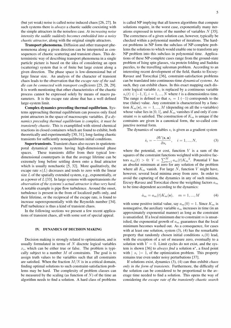
is called NP implying that all known algorithms that computesolutions require, in the worst case, exponentially many iter-ations expressed in terms of the number of variables N [35].The correctness of a given solution can, however, typically bechecked within a polynomial number of iterations. The hard-est problems in NP form the subclass of NP-complete prob-lems the solutions to which would enable one to transform anyNP problem into this subclass in polynomial time. Applica-tions of these NP-complete cases range from the ground-stateproblem of Ising spin glasses, via protein folding and Sudokupuzzles, to the travelling salesman problem. According to aninteresting recent development of the field, thanks to Ercsey-Ravasz and Toroczkai [36], constraint-satisfaction problemscan be translated into continuous-time dynamical systems. Assuch, they can exhibit chaos. In this exact mapping each dis-crete logical variable xi is replaced by a continuous variablesi(t) ∈ [−1, 1], i = 1, ..., N where t is a dimensionless time.The range is defined so that si = 1 (−1) corresponds to thetrue (false) value. Any constraint is characterized by a func-tion Km(s), m = 1, ...,M (depending on all the s-variables)whose value lies in [0, 1], and Km vanishes if and only if con-straint m is satisfied. The construction of Km is unique if thecontraints are given in a canonical form, the so-called con-junctive normal form.

The dynamics of variables si is given as a gradient system

si = −∂V (s,a)

∂si, i = 1, ..., N, (3)

where the potential, or cost, function V is a sum of thesquares of the constraint functions weighted with positive fac-tors am(t) > 0: V =

∑Mm=1 am(t)Km

2. Potential V hasan absolut minimum at zero for any solution of the problemwhere all Km vanish. For large N , function V might have,however, several local minima away from zero. In order toavoid the capturing of the dynamics in any of such minima,Ercsey-Ravasz and Toroczkai chose the weigthing factors amto be time-dependent according to the dynamics:

am = am(t)Km(s), m = 1, ...,M (4)

with some positive initial value, say am(0) = 1. Since Km isnonnegative, the auxiliary variable am increases in time (in anapproximately exponential manner) as long as the constraintis unsatisfied. If a local minimum due to constraintm is unsat-isfied, the exponential growth of am guarantees that the localminimum becomes washed out. As a consequence, for caseswith at least one solution, system (3), (4) has the remarkableproperty that randomly chosen initial conditions si(0) lead,with the exception of a set of measure zero, eventually to asolution with V = 0. Limit cycles do not exist, and the sys-tem is shown [36] to always find a solution s∗, a fixed pointwith | si |= 1, of the optimization problem. This propertyremains true even under noisy perturbations [37].

If solutions exist, dynamics (3), (4) can thus exhibit chaosonly in the form of transients. Furthermore, the difficulty ofthe solution can be considered to be proportional to the av-erage time needed to find a solution. This opens the way ofconsidering the escape rate of the transiently chaotic search

6

dynamics to be a measure of the hardness of the problem in-stance.

As an example to illustrate the search dynamics, we showa Sudoku puzzle [38] and the characteristic time-dependenceof some of the s-variables in Fig. 5. In Sudoku, one has tofill in the cells of a 9 × 9 grid with integers 1 to 9 such that inall rows, all columns, and in nine 3 × 3 blocks every digit ap-pears exactly once, while a set of given isolated digits shouldalso be taken into account (see left panel of Fig. 5). Theserules and the given digits determine both N and M , the num-ber of independent variables (each empty cell is representedby at most 9 independent logical variables) and constraints,respectively. Sudoku puzzles are designed to have unique so-lutions. The right panel of Fig. 5 shows the time evolutionof the continuous-time dynamics of the 3 × 3 grid formedby rows 4-6 and columns 7-9. In each cell there is only ones-variable which converges to 1, the one representing the so-lution, all the others converge to −1 since they correspondto false digits. The dynamics preceding the asymptotic stateis rather complex: all s-values change irregularly, exhibitinglong chaotic transients. The solution can be seen to be foundin this example after about 150 time units. In other runs evenmuch longer search times are found. In an ensemble of 104

randomly chosen inital conditions the probability that the dy-namics has not found the solution by time t follows the rule(1), and the escape rate of the underlying chaotic saddle isobtained to be κ = 0.00026 (1/κ = 3850) [38].

FIG. 5: Transient chaos preceding the finding of the Sudoku solu-tion in the search dynamics (3), (4). The puzzle given in the leftpanel is one of the hardest: with the 21 given digits, it correspondsto N = 257, M = 2085. The time-dependence of the variablessaij (representing digit a, colored as in the color bar on the right) incell i, j is shown in the right panel. In each cell there are 9 runningtrajectories but many of them are on top of each other close to −1.Courtesy of M. Ercsey-Ravasz and Z. Toroczkai.

The authors of [38] also showed that the escape rate of apuzzle correlates very well with human difficulty ratings. Fourcategories predefined by the public: easy, medium, hard, andultra-hard turn out to be related to the escape rate via a loga-rithmic law. η = − log10 κ values correspond to them in theranges 0 < η ≤ 1, 1 < η ≤ 2, 2 < η ≤ 3, and 3 < η ≤ 4,respectively. Puzzles with η > 4 are not known.

A further interesting property of the escape rate of randomdecision making problems is that in cases when the numberN of independent s-variables can change in a broad range,the escape rate is found [36] to decrease as a power of N

κ(N) = bN−β (5)

with an exponent β ≈ 5/3. The transient dynamics of deci-sion making is thus supertransient. This law holds for a fixedvalue ofM/N = 4.25 in the critical region, and illustrates thatthe escape rate κ(N) is a dynamical measure of optimizationhardness (thus capable of separately characterising individualinstances), while M/N is a static one only. (In the Sudokuproblem, which is also high-dimensional, this means that notonly the number of the preselected digits is important, but alsotheir positioning pattern.)

Equation (5) also implies that the scaling of the averagecontinuous-time (≈ 1/κ) is polynomial. Nonetheless, theexponential scaling characteristic to NP-complete problemsdoes not disappear, but appears when measuring the num-ber of integration steps needed (using adaptive Runge-Kuttamethods).

V. VOLCANIC ASH DISPERSION

The volcanic eruption of Eyjafjallajokull on Iceland in 2010lead to concerns that volcanic ash would damage aircraft en-gines, and the controlled airspace of many European countrieswas closed resulting in the largest air-traffic shut-down sinceWorld War II. The closures caused millions of passengers tobe stranded not only in Europe, but across the world. Notmuch later, the Fukushima accident (2011) lead to increasedpublic concern regarding pollutant spreading from industrialaccidents. These recent events underlined the need for inves-tigating pollutant dispersion in the atmosphere. Aerosol par-ticles from different sources may be advected far away fromtheir initial position and may cause air pollution episodes atdistant locations.

Current numerical capacity enables us to monitor individ-ual aerosol particles one by one. These trajectories turn outto be chaotic, and an ensemble of trajectories can be used topredict statistical properties, e.g. the average deposition dy-namics.

In order to track individual aerosol particles with realisticsize and density, the equation of motion for the particle trajec-tory r(t) is derived from Newton’s equation. Scale analysisreveals that the horizontal velocity of a small aerosol parti-cle takes over the actual local wind speed practically instanta-neously, whereas vertically the terminal velocity w should beadded to the vertical velocity component of air [39, 40]. w de-pends on the radius r and density ρp of the spherical particle,as well as, on the density ρ and viscosity ν of the air at thelocation of the particle:

r = v(r(t), t) + wn, (6)

where v(r, t) is the wind field at point r and time t, and n isthe vertical unit vector pointing downwards. Realistic aerosolparticles not falling out within hours are of radius of at most12 µm, and have a density of about ρp = 2000 kg/m3. Forthem, Stokes’ law is valid during the full motion, and hencethe terminal velocity is w = 2ρpr

2/(9ρνg). As an input todispersion simulations, the reanalysis data of measured windfields can be used, which are accessible e.g., in the ERA-Interim database [41]. The wind velocity at the actual loca-

7

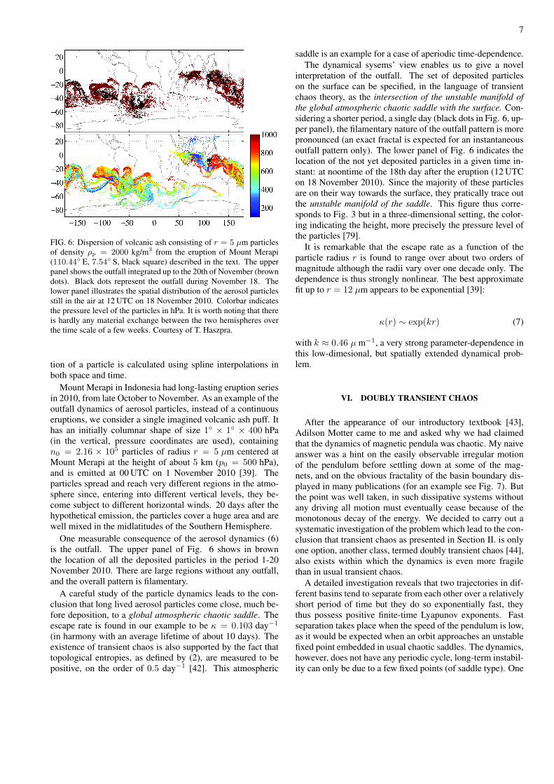
FIG. 6: Dispersion of volcanic ash consisting of r = 5 µm particlesof density ρp = 2000 kg/m3 from the eruption of Mount Merapi(110.44◦ E, 7.54◦ S, black square) described in the text. The upperpanel shows the outfall integrated up to the 20th of November (browndots). Black dots represent the outfall during November 18. Thelower panel illustrates the spatial distribution of the aerosol particlesstill in the air at 12 UTC on 18 November 2010. Colorbar indicatesthe pressure level of the particles in hPa. It is worth noting that thereis hardly any material exchange between the two hemispheres overthe time scale of a few weeks. Courtesy of T. Haszpra.

tion of a particle is calculated using spline interpolations inboth space and time.

Mount Merapi in Indonesia had long-lasting eruption seriesin 2010, from late October to November. As an example of theoutfall dynamics of aerosol particles, instead of a continuouseruptions, we consider a single imagined volcanic ash puff. Ithas an initially columnar shape of size 1◦ × 1◦ × 400 hPa(in the vertical, pressure coordinates are used), containingn0 = 2.16 × 105 particles of radius r = 5 µm centered atMount Merapi at the height of about 5 km (p0 = 500 hPa),and is emitted at 00 UTC on 1 November 2010 [39]. Theparticles spread and reach very different regions in the atmo-sphere since, entering into different vertical levels, they be-come subject to different horizontal winds. 20 days after thehypothetical emission, the particles cover a huge area and arewell mixed in the midlatitudes of the Southern Hemisphere.

One measurable consequence of the aerosol dynamics (6)is the outfall. The upper panel of Fig. 6 shows in brownthe location of all the deposited particles in the period 1-20November 2010. There are large regions without any outfall,and the overall pattern is filamentary.

A careful study of the particle dynamics leads to the con-clusion that long lived aerosol particles come close, much be-fore deposition, to a global atmospheric chaotic saddle. Theescape rate is found in our example to be κ = 0.103 day−1

(in harmony with an average lifetime of about 10 days). Theexistence of transient chaos is also supported by the fact thattopological entropies, as defined by (2), are measured to bepositive, on the order of 0.5 day−1 [42]. This atmospheric

saddle is an example for a case of aperiodic time-dependence.The dynamical sysems’ view enables us to give a novel

interpretation of the outfall. The set of deposited particleson the surface can be specified, in the language of transientchaos theory, as the intersection of the unstable manifold ofthe global atmospheric chaotic saddle with the surface. Con-sidering a shorter period, a single day (black dots in Fig. 6, up-per panel), the filamentary nature of the outfall pattern is morepronounced (an exact fractal is expected for an instantaneousoutfall pattern only). The lower panel of Fig. 6 indicates thelocation of the not yet deposited particles in a given time in-stant: at noontime of the 18th day after the eruption (12 UTCon 18 November 2010). Since the majority of these particlesare on their way towards the surface, they pratically trace outthe unstable manifold of the saddle. This figure thus corre-sponds to Fig. 3 but in a three-dimensional setting, the color-ing indicating the height, more precisely the pressure level ofthe particles [79].

It is remarkable that the escape rate as a function of theparticle radius r is found to range over about two orders ofmagnitude although the radii vary over one decade only. Thedependence is thus strongly nonlinear. The best approximatefit up to r = 12 µm appears to be exponential [39]:

κ(r) ∼ exp(kr) (7)

with k ≈ 0.46 µ m−1, a very strong parameter-dependence inthis low-dimesional, but spatially extended dynamical prob-lem.

VI. DOUBLY TRANSIENT CHAOS

After the appearance of our introductory textbook [43],Adilson Motter came to me and asked why we had claimedthat the dynamics of magnetic pendula was chaotic. My naiveanswer was a hint on the easily observable irregular motionof the pendulum before settling down at some of the mag-nets, and on the obvious fractality of the basin boundary dis-played in many publications (for an example see Fig. 7). Butthe point was well taken, in such dissipative systems withoutany driving all motion must eventually cease because of themonotonous decay of the energy. We decided to carry out asystematic investigation of the problem which lead to the con-clusion that transient chaos as presented in Section II. is onlyone option, another class, termed doubly transient chaos [44],also exists within which the dynamics is even more fragilethan in usual transient chaos.

A detailed investigation reveals that two trajectories in dif-ferent basins tend to separate from each other over a relativelyshort period of time but they do so exponentially fast, theythus possess positive finite-time Lyapunov exponents. Fastseparation takes place when the speed of the pendulum is low,as it would be expected when an orbit approaches an unstablefixed point embedded in usual chaotic saddles. The dynamics,however, does not have any periodic cycle, long-term instabil-ity can only be due to a few fixed points (of saddle type). One

8

FIG. 7: Part of the basin structure of a magnetic pendulum with threemagnets at the corner of a regular horizontal triangle of unit edgelength around the origin. A part of the plane of initial positions isshown, where points with vanishing initial velocity are colored ac-cording to the magnet in which neighborhood the pendulum settlesdown. Most observer would consider this pattern to be fractal. Cour-tesy of G. Karolyi.

observes, nevertheless, that during the period of rapid sepa-ration the trajectories wander erratically in the vicinity of aset that plays the role of a chaotic saddle. This set can beestimated from the positions where the trajectories separateexponentially from each other. However, this set consists ofonly pieces of trajectories in the phase space and – in contrastto usual saddles, like e.g., the one shown in Fig. 1 – is not aninvariant set of orbits. Moreover, this set manifests itself onlyduring the period of exponential separation, which motivatesus to refer to it as a transient chaotic saddle.

This view is supported by the observation of the individuallifetimes spent far away from any attractor obtained for trajec-tories which started on a straight line with zero initial velocity.This function is higly irregular, and appears to exhibit a fewisolated infinitely high peaks only (in contrast to traditionalsystems where infinities sit on a fractal set). In our case sub-sequent magnifications indicate that the set of long lifetimesbecomes increasingly sparse at sufficiently small scales.

This leads us to the conclusion that perhaps a time-dependent escape rate would provide a proper characteriza-tion of the dynamics. We define [44] this as the instantaneousrate κ(t) of decay of the fraction p(t) of still unsettled trajec-tories at time t

p(t) = −κ(t)p(t). (8)

Numerical results indicate that κ(t) is an exponentially in-creasing function in this example. The survival probabil-ity thus decays superexponentially, i.e., the escape dynamicsspeeds up as times goes on.

In harmony with the time-dependence of the escape rate,we find that the fractality of the basin boundary is scale-dependent. Considering smaller and smaller scales, the fractal

FIG. 8: Blowing up the basin structure. Left panel: magnification ofa small square from the most fractal-looking lower left quadrant ofFig. 7. Right panel: magnification of a small square of the left panel.The dilution of fractality can be seen by naked eye. Courtesy of G.Karolyi.

dimension of the set separating the different colors is found todecrease and tend to unity [44]. This can indeed be seen whenconsidering subsequent magnifications of Fig. 7 as illustartedby Fig. 8.

It is interesting to observe that the character of chaos imme-diately changes when driving is added. By moving the plateof the magnets up and down in a sinusoidal manner, unstableperiodic orbits immediately appear, and the long term dynam-ics is governed by a usual chaotic saddle (in coexistence withperiodic attractors). For small driving amplitudes, the time-dependent escape rate (8) initially increases, but then levelsoff at a finite constant value, and the crossover period shrinkswith the amplitude.

In summary, our principal results are that in undriven sys-tems: (i) the measured dimension of the basin boundaries canbe noninteger and the finite-time Lyapunov exponents can bepositive over finite scales but neither holds true asymptoti-cally; (ii) the basin boundaries have (asymptotic) integer frac-tal dimensions; (iii) the survival probability outside the attrac-tors changes dramatically, characterized by a time-dependentescape rate; (iv) transient behavior is governed by a transientchaotic saddle that is prominent over a specific energy inter-val. This doubly transient chaos appears to be the genericform of chaos in autonomous (nondriven) dissipative systems,with the double pendulum and many every-day phenomena asexamples.

VII. DYNAMICAL SYSTEMS WITHABSORPTION/EXPLOSION

Certain physical problems related to wave dynamics in theshort wavelength limit can be represented by particles movingalong simple trajectories but carrying with them certain phys-ical quantities which change in time according to some rule.One example is the decay of sound intensity in hall acous-tics, which can be understood by considering sound rays (par-ticles) bouncing with constant velocity within a billiard (thehall) which loose a portion of a quantity (the energy) carriedwith them upon each collision with the wall. This loss of en-ergy corresponds to sound attenuation, or absorption in gen-

9

eral. In such systems it is not the particles (matter) what es-capes rather the energy content, a quantity carried along withthe particles.

The usual dynamical systems’ approach should somewhatbe broadened for a proper description of such problems. Con-sider a discrete-time representation ~xn+1 = f(~xn), a properPoincare map of a time-continuous flow. One can fully recon-struct the continuous-time dynamics if the return time distri-bution τ(~x) [chosen as the time between ~x and ~x′ ≡ f(~x)]is known and the sum of return times is followed along themap trajectory [25]. The novel feature is that besides the re-turn time, the evolution of an intensity-like quantity J shouldalso be monitored. This quantity can be represented to changeonly upon intersections with the Poincare surface, when itsvalue becomes suddenly smaller. The amount of this changeis specified by the distribution R(~x) of reflection coefficients,a quantity assumed to be known on the Poincare surface (justlike τ(~x)). Instead of the usual map f , one then follows anextended map fext which implies extending the map’s phasespace ~xn by two further variables tn and Jn: the time at in-tersection n with the surface, and the intensity just before thisintersection. The extended map thus reads as

fext :

~xn+1 = f(~xn),tn+1 = tn + τ(~xn),Jn+1 = JnR(~xn).

(9)

Instead of indiviual trajectories in the extended phase space,it is worth studying here also an ensemble of trajectories, andtheir energy density ρ(~x, t). In analogy with the problemof room acoustics, we consider closed chaotic maps f(~xn)and find [45] that for any smooth initial intensity distributionρ(~x, t = 0) there is an overall exponential decay, multipliedby a distribution ρc(~x) depending only on the spatial coordi-nates so that for long times

ρ(~x, t) ∼ e−κtρc(~x). (10)

Exponent κ > 0 is called again the escape rate but, remember,it is a measure of the energy escape since there is no particleescape as map f is assumed to be closed [80]. Both κ andρc are found to be independent of initial conditions. Writing(10) as ρc(~x) ∼ eκtρ(~x, t) shows that ρc is kind of a limitdistribution obtained by compensating for the energy loss byhomogeneously injecting energy exactly at the rate of κ. Den-sity ρc is terefore called the conditionally invariant density(c-measure) in analogy with a quantity introduced as the den-sity of points conditioned to escape after a long stay only inusual open systems with transient chaos [46]. c-ensity ρc canbe normalized to unity over the phase space of map f . Thec-density is found to be a complicated fractal measure with anontrivial information dimension, as illustrated by Fig. 9. Thefilamentary pattern suggests that this density is concentratedon the unstable manifold of the intensity dynamics (as in usualtransient chaos), and one can also find the underlying chaoticsaddle in the extended map.

Within this extended set-up one can even find a physicalinterpretation for negative escape rates. Optical microcavi-ties provide a repesentative example of such systems. Lasing

FIG. 9: Energy escape in a two-dimensional billiard. Left panel:billiard with partial reflectivity, the width of the ray is proportionalto its intensity (J). The reflection coefficient R = R∗ = 0.1 inthe gray boundary interval, at other locations there is no absorption:R = 1. Right panel: c-density with color coding. The correspondingescape rate is κ = 0.058. Birkhoff coordinates ~x = (s, p = sin θ)are used, where s is the arc length along the boundary and θ is thecollision angle. Courtesy of E.G. Altmann and J.S.E. Portela.

modes are induced by the gain medium present in the cavi-ties and only long-living light rays are able to profit from thisgain. For strong enough gain, when the reflection coefficientis larger than unity: R(~x) > 1, in certain regions at least, theoverall intensity ρ(~x, t) increases in time, in an exponentialfashion [47]. Eq. (10) remains thus valid, just with a negativeκ. Quantity −κ can be called the explosion rate. It is perhapsa surprise that the c-density does not lose its fractal measureproperty as Fig. 10 demonstrates.

FIG. 10: Energy explosion in the same billiard as in Fig. 9. Leftpanel: billiard with a gain region in the middle (gray disc, markedby g), the width of the ray is proportional to its intensity (J). Thereflection coefficient upon collision with the wall is R = eτg ≤ 1where τg is the time the trajectory spends in the gain region. Rightpanel: c-density with color coding. The corresponding explosion rateis −κ = 0.215. Courtesy of E.G. Altmann and J.S.E. Portela.

It is instructive to see that there exists a unified frameworkvalid both for absorbing and exploding cases that also showshow κ and the c-density are related. For invertible f -dynamicsthis can be written as a discrete-time Perron-Frobenius-typeequation [45, 47] (see also [48]) acting on the density functionρn of the extended map as

ρn+1(~x′) = eκτ(~x)R(~x)ρn(~x)

| Df (~x) |. (11)

Here Df (~x) is the Jacobian of the Poincare map f at thephase space coordinate ~x (in the billiard examples, of course,

10

Df (~x) = 1). Iteration scheme (11) expresses, in a more ad-vanced form, the compensation mechanism mentioned abovein relation to (10): when compensating escape (explosion) byinjecting (extracting) energy via a multiplication with eκτ(~x)

per iteration, a time-independent limit-distribution ρ∞(~x) isreached. This only happens if κ is the valid escape rate,and then the limit disribution is the corresponding c-density:ρ∞(~x) = ρc(~x). Integrating (11) over ~x′ with the c-densityon both sides, and using the normalization of ρc, one finds

< eκτR >c= 1, (12)

where the average is taken with respect to the c-measure. Thisexpresses an intimate relation: κ and ρc are selfconsistentlyadjusted so that the average of the compensated reflection co-efficient eκτR should be unity (a sign of stationarity) when theavarege is taken just with the c-measure. Quantities κ and ρccan also be considered as the parameter making the eigenvalueof the operator defined by (11) to be unity and the eigenfunc-tion belonging to this largest eigenvalue, respectively. It isimmediate from (12) that for R > 1, in sufficiently extendedreagions at least (i.e., the case of explosion), κ must be nega-tive.

One can also find [45, 47] a general relation between thefractality of ρc, the distributions τ(~x), R(~x), and propertiesof the extended map. The information dimension D(1)

1 of thechaotic saddle along the unstable foliation of two-dimensionalextended maps can be expressed as

D(1)1 = 1− κτ + lnR

λ, (13)

where the averages denoted by overbars are taken over thechaotic saddle of this map. It is remarkable that the dimensioncan be expressed in such a simple way. Besides the escaperate κ and the positive average Lyapunov exponent λ only theaverages τ of the return times and lnR of the logarithm ofthe reflection coefficients appear[81]. This result is an exten-sion of the Kantz-Grassberger formula D(1)

1 = 1−κ/λ, validfor the partial dimension in usual transient chaos. The beautyof this generic and simple relation connecting fragile (sinceD

(1)1 < 1) fractality and dynamics, which I first saw during

that 1985 Dynamics Days, certainly contributed to my contin-uous attraction towards transient chaos.

VIII. OUTLOOK

I would like to end with a brief summary of furthertransient-chaos related subjects, which might be at least asinteresting as the ones just presented in some detail above.Leaky dynamical systems arise when artificial holes are in-troduced into closed dynamics, and the study of the resulting

transient dynamics reveals relevant features of the closed dy-namics, including Poincare recurrences [48]. Almost invari-ant sets are subsets of larger systems points of which remainbound to this subset for a long time. They are thus naturalcandidates for characterizing Lagrangian coherent structures[19], and other environment-related phenomena [49]. Tran-sient chaos theory can also be used to understand the origin oftransients and extreme events in excitable systems [50, 51],long spatio-temporal transients in chimera states [52, 53],memory effects in particle dispersion in open flows [54], andto gain a deeper insight into the nature of turbulence [55].Recent developments in classical chaotic scattering includethe investigation of the ray dynamics in optical metamaterials[56], of escape in celestial mechanics [57, 58] and in medi-cally relevant fluid flows [59, 60], and a basic understandingof the structure of chaotic saddles in higher dimensions [61–64].

Snapshot chaotic saddles and attractors exist in aperiodi-cally driven system [65], and represent instantaneous states ofensembles of trajectories. A novel observation of recent yearsis that they are uniquely defined not only in noisy systems [66]but also in the presence of smooth driving that might even bea one-sided temporal shift of some parameters. This prop-erty makes the concept very well suited for an application inclimate dynamics [67–69]. The observed robust existence ofchaotic snapshot attractors over a wide range is a consequenceof the presence of transient chaos in the undriven system:the dynamics on snapshot attractors might thus be considereddriving-induced-chaos (in analogy with noise-induced-chaos).

Quantum aspects cannot be left without a very short men-tion. Features related to open channels in quantum systemsappear in properties such as, e.g., the fractal distribution ofeigenstates [70], the fractal Weyl’s law [71, 72], and quan-tum transport [73], including transport in graphene [74]. Theinvestigation of these quantum properties is also subject of ac-tive recent research (see e.g., [48, 75, 76]).

My final conclusion can only be: Keep an eye on the poten-tial appearance of transient chaos since this phenomenon isan inexhaustible source of challenge and inspiration.

ACKNOWLEDGMENTS

This work was supported by OTKA Grant No. NK100296.The support of the Alexander von Humboldt Foundation is ac-knowledged. Special thank is due to E. Altmann, M. Ercsey-Ravasz, T. Haszpra, G. Karolyi, J.S.Portela, and Z. Toroczkaiwho helped with preparation of figures for this paper. Insight-ful discsussions with them and with T. Bodai, A. Daitche, G.Drotos, U. Feudel, M. Ghil, K. Guseva, G. Haller, C. Jung, Y.-C. Lai, A. Motter, and M. Vincze are deeply acknowledged.

[1] T. Tel, in: Directions in Chaos, Vol .3, ed.: Bai-lin Hao (WorldScientific, Singapore, 1990) pp. 149-221; T. Tel, in: STATPHYS

19: The Proceedings of the 19th IUPAP Conference on Statisti-

11

cal Physics (World Scientific, Singapore, 1996), pp. 346-362.[2] Y.-C. Lai and T. Tel, Transient Chaos, Complex Dynamics on

Finite-Time Scales (Springer, New York, 2011)[3] T. Tel, Phys. Rev. A 36, 1502 (1987)[4] H. Kantz and P. Grassberger, Physica D 17, 75 (1985).[5] C. Grebogi, E. Ott and J. Yorke, Phys. Rev. Lett. 48, 1507

(1982); Physica D 7, 181 (1983).[6] C. Grebogi, E. Ott and J. Yorke, Phys. Rev. Lett. 50, 935 (1983)[7] C. Jung, T. Tel, and E. Ziemniak, Chaos 3, 555 (1993)[8] H. Aref, J. Fluid. Mech. 143, 1 (1984)[9] J.C. Sommerer, H. Ku, and H. Gilreath, Phys. Rev. Lett 77,

5055 (1996)[10] M. Van Dyke, An Album of Fluid Motion (Parabolic Press, Stan-

ford, 1988).[11] F. Ladrappier and L.-S. Young, Commun. Math. Phys. 117, 529

(1989).[12] J. Jacobs, E. Ott, T. Antonsen, and J. Yorke, Physica D 110, 1

(1997)[13] Z. Neufeld and T. Tel, Phys. Rev. E 57, 2832 (1998)[14] I. Scheuring, T. Czaran, P. Szabo, G. Karolyi, and Z. Toroczkai,

Orig. Life Evolution of Biosphere 133, 319 (2002)[15] Z. Neufeld and E. Hernandez-Garcia, Chemical and Biologi-

cal Processes in Fluid Flows (Imperial College Press, London,2010)

[16] S.E. Newhouse and T. Pignataro, J. Stat. Phys. 72, 1331 (1993)[17] B.R. Hunt and E. Ott, Chaos 25, this issue (2015)[18] G. Haller and G. Yuan, Physica D 147, 352 (2000)[19] G. Haller, Annu. Rev. Fluid. Mech 47, 137 (2015)[20] M. Sandulescu, C.E. Lopez, E. Hernandez-Garcia, and U.

Feudel, Ecol. Complex. 5, 228 (2008)[21] C.S. Harrison, D.A. Siegel, and S. Mitarai, Mar. Ecol. Prog. Ser.

472, 27 (2013)[22] E.T. Kai et al., Proc. Nat. Acad. Sci. 106, 8245 (2009)[23] E. Ott, Chaos in Dynamical Systems (Cambridge University

Press, Cambridge, 1993, 2002)[24] E. Ott, C. Grebogi and J. Yorke, Phys. Rev. Lett. 64, 1996

(1990)[25] P. Gaspard, Chaos, Scattering and Statistical Mechanics (Cam-

bridge University Press, Cambridge, 1998)[26] M. Iansity, Q. Hu, R.M. Westerveel and M. Tinkham, Phys.

Rev. Lett. 55, 746 (1985)[27] Y.-C. Lai, Z. Liu, L. Billings, and I.B. Schwartz, Phys. Rev. E,

026210 (2003)[28] J. Vollmer, Physics Reports 372, 131 (2002)[29] R. Klages, Macroscopic Chaos, Fractals and Transport in

Nonequilibrium Statistical Mechanics (World Scientific, Singa-pore, 2007)

[30] S. Scott, B. Peng, A. Tomlin, and K. Showalter, J. Chem. Phys.94, 1134 (1991)

[31] J. Wang, P.G. Sorensen, and F. Hynne, J. Phys. Chem. 98, 725(1994)

[32] Y.-H. Do and Y.-C. Lai, Phys. Rev. Lett. 91, 224101 (2003)[33] J. P. Crutchfield and K. Kaneko, Phys. Rev. Lett. 60, 2715

(1988);[34] B. Hof, A. de Lozar, D.J. Kuik, and J. Westerweel, Phys. Rev.

Lett. 101, 214501 (2009)[35] M.R. Garey and D.S. Johnson, Computers and Intractability: A

Guide to the Theory of NP-Completness (W.H. Freeman, NewYork, 1990)

[36] M. Ercsey-Ravasz and Z. Toroczkai, Nature Physics 7, 966(2011)

[37] R. Sumi, B. Molnar and M. Ercsey-Ravasz, Eur. Phys. Lett. 106,40001 (2014)

[38] M. Ercsey-Ravasz and Z. Toroczkai, Scientific Reports 2, 725

(2012)[39] T. Haszpra, and T. Tel, Nonlinear Processes in Geophysics, 20,

867 (2013)[40] T. Haszpra and A. Horanyi, Idojaras, Quaterly J. of the Hungar-

ian Met. Service 118, 335 (2014)[41] D. P. Dee et al., Quarterly Journal of the Royal Meteorological

Society 137, 553 (2011)[42] T. Haszpra, and T. Tel, Journal of the Atmospheric Sciences 70,

4030 (2013)[43] T. Tel and M. Gruiz, Chaotic Dynamics (Cambridge University

Press, Cambridge, 2006)[44] A.E. Motter, M. Gruiz, G. Karolyi, and T. Tel, Phys. Rev. Lett.

111, 194101 (2013)[45] E.G. Altmann, J.S.E. Portela, and T. Tel, Phys. Rev. Lett. 111

144101 (2013).[46] G. Pianigiani and J. A. Yorke, Trans. Amer. Math. Soc. 252,

351 (1979).[47] E.G. Altmann, J.S.E. Portela, and T. Tel, Europhys. Lett. 109,

30003 (2015)[48] E.G. Altmann, J.S.E. Portela, and T. Tel, Rev. Mod. Phys. 85

869 (2013)[49] G. Froyland, R.M. Stuart, and E. van Sebille, Chaos 24, 033126

(2014)[50] H.-L. Zou, M.-L. Li, C. H. Lai, and Y.-C. Lai, Phys. Rev. E 86,

066214 (2012)[51] R. Karnatak, G. Ansmann, U. Feudel, and K. Lehnertz, Phys.

Rev. E 90, 022917 (2014)[52] M. Wolfrum and O.E. Omelchenko, Phys. Rev. E. 84,

015201(R) (2011)[53] D.P. Rosin, D. Rontani, N.D. Haynes, E. Scholl, and D.J. Gau-

thier, Phys. Rev. E 90, 030902(R) (2014)[54] A. Daitche and T. Tel, New. J. Phys. 16, 073008 (2014)[55] T. Kreilos, B. Eckhardt, and T. M. Schneider, Phys. Rev. Lett.

112, 044503 (2014)[56] X. Ni and Y.-C. Lai, Chaos 21, 033116 (2011)[57] T. Kovacs, Gy. Bene, and T. Tel, Mon. Not. Royal. Astron. Soc.

414, 2275 (2011)[58] T. Kovacs and Zs. Regaly, Astrophys. J. Lett. 798, L9 (2015)[59] A.B. Schelin, Gy. Karolyi, A.P.S. de Moura, N. Booth, C. Gre-

bogi, Computers in Biology and Medicine 42, 276 (2012)[60] G. Zavodszky, Gy. Karolyi, Gy. Paal, J. Theor. Biol. 368, 95

(2015)[61] F. Gonzales and C. Jung, J. Phys. A 45, 265102 (2012)[62] F. Gonzales, G. Drotos, and C. Jung, J. Phys. A 47, 045101

(2014)[63] G. Drotos, F. Gonzales Montoya, C. Jung, and T. Tel, Phys.

Rev. E 90, 022906 (2014)[64] E.E. Zotos, Nonlinear Dyn. 76, 1301 (2014)[65] P.J. Romeiras, C. Grebogi, and E. Ott, Phys. Rev. A 41, 784

(1990)[66] T. Bodai, E. G. Altmann, and A. Endler, Phys. Rev. E 87,

042902 (2013)[67] M. Ghil, M.D. Chekroun, and E. Simonnet, Physica D 237,

2111 (2008)[68] T. Bodai and T. Tel, Chaos 22, 023110 (2012)[69] G. Drotos, T. Bodai, and T. Tel, J. Climate 28, 3275 (2015)[70] J.M. Pedrosa, G.G. Carlo, D.A. Wisniacki, and L. Ermann,

Phys. Rev. E 79, 016215 (2009)[71] S. Nonnenmacher, Nonlinearity 24, R123 (2011)[72] M. Novaes, Journal of Physics A 46, 143001 (2013)[73] R. Yang, L. Huang, Y.-C. Lai, C. Grebogi, and L. M. Pecora,

Chaos 23, 013125 (2013).[74] G.-L. Wang, L. Ying, Y.-C. Lai, and C. Grebogi, Phys. Rev. E

87, 052908 (2013).

12

[75] M. Schonwetter and E. G. Altmann, Phys. Rev. E 91, 012919(2015)

[76] H. Cai and J. Wiersig, Rev. Mod. Phys. 87, 61 (2015)[77] Such sets of noninvertible systems are called chaotic repellers.[78] There might be a deviation from (1) for very large times, too,

due to, e.g. particles sticking to the obstacle’s surface.[79] For simplicity, chaotic diffusion and precipitation was not taken

into account in the simulation shown in Fig. 6; the inclusion ofthese effects would not change the picture qualitatively [39].

[80] When map f is open, one can define two escape rates: one forthe energy, another one (the usual escape rate) for particles.

[81] For the other partial dimension one also needs to know the nega-tive Lyapunov exponent λ′, and finds it asD(2)

1 = −D(1)1 λ/λ′.

The information dimension D(1)1 of the saddle and D1c of the

c-measure are than D(1)1 = D

(1)1 +D

(2)1 and D1c = 1 +D

(2)1 ,

respectively.