1 robust portfolio optimization using second-order cone ...chapter_1.pdf · mean variance frontier...
TRANSCRIPT
© 2009 Elsevier Limited. All rights reserved.Doi:10.1016/B978-0-12-374952-9.00001-4.
2010
Robust portfolio optimization using second-order cone programming Fiona Kolbert and Laurence Wormald
1
Executive Summary
Optimization maintains its importance within portfolio management, despite many criticisms of the Markowitz approach, because modern algorithmic approaches are able to provide solutions to much more wide-ranging optimization problems than the classical mean – variance case. By setting up problems with more general constraints and more flexible objective functions, investors can model investment realities in a way that was not available to the first generation of users of risk models.
In this chapter, we review the use of second-order cone programming to handle a number of economically important optimization problems involving:
● Alpha uncertainty ● Constraints on systematic and specific risks ● Fund of funds with multiple active risk constraints ● Constraints on risk using more than one risk model ● Combining different risk measures
1.1 Introduction
Despite an almost-continuous criticism of mathematical optimization as a method of constructing investment portfolios since it was first proposed, there are an ever-increasing number of practitioners of this method using it to man-age more and more assets. Given the fact that the problems associated with the Markowitz approach are so well known and so widely acknowledged, why is it that portfolio optimization remains popular with well-informed investment professionals?
The answer lies in the fact that modern algorithmic approaches are able to pro-vide solutions to much more wide-ranging optimization problems than the clas-sical mean – variance case. By setting up problems with more general constraints and more flexible objective functions, investors can model investment realities in a way that was not available to the first generation of users of risk models.
In particular, the methods of cone programming allow efficient solutions to problems that involve more than one quadratic constraint, more than one
06_P374952_Ch01.indd 306_P374952_Ch01.indd 3 9/15/2009 5:13:48 PM9/15/2009 5:13:48 PM
Optimizing Optimization4
quadratic term within the utility function, and more than one benchmark. In this way, investors can go about finding solutions that are robust against the failure of a number of simplifying assumptions that had previously been seen as fatally compromising the mean – variance optimization approach.
In this chapter, we consider a number of economically important optimiza-tion problems that can be solved efficiently by means of second-order cone programming (SOCP) techniques. In each case, we demonstrate by means of fully worked examples the intuitive improvement to the investor that can be obtained by making use of SOCP, and in doing so we hope to focus the discussion of the value of portfolio optimization where it should be on the proper definition of utility and the quality of the underlying alpha and risk models.
1.2 Alpha uncertainty
The standard mean – variance portfolio optimization approach assumes that the alphas are known and given by some vector α . The problem with this is that generally the alpha predictions are not known with certainty — an investor can estimate alphas but clearly cannot be certain that their predictions will be cor-rect. However, when the alpha predictions are subsequently used in an optimi-zation, the optimizer will treat the alphas as being certain and may choose a solution that places unjustified emphasis on those assets that have particularly large alpha predictions.
Attempts to compensate for this in the standard quadratic programming approach include just reducing alphas that look too large to give more con-servative estimates and imposing constraints such as maximum asset weight and sector weight constraints to try and prevent any individual alpha estimate having too large an impact. However, none of these methods directly address the issue and these approaches can lead to suboptimal results. A better way of dealing with the problem is to use SOCP to include uncertainty information in the optimization process.
If the alphas are assumed to follow a normal distribution with mean α * and known covariance matrix of estimation errors Ω , then we can define an ellipti-cal confidence region around the mean estimated alphas as:
( ) ( )α α α α� ��* *T Ω 1 2− k
There are then several ways of setting up the robust optimization problem; the one we consider is to maximize the worst-case return for the given confi-dence region, subject to a constraint on the mean portfolio return, α p . If w is the vector of portfolio weights, the problem is:
Maximize Min portfolio varianceT( ( ) )w α �
06_P374952_Ch01.indd 406_P374952_Ch01.indd 4 9/15/2009 5:13:49 PM9/15/2009 5:13:49 PM
Robust portfolio optimization using second-order cone programming 5
subject to
( ) ( )α α α α� � ��* *T Ω 1 2k
α α*Tw p�
e w 1T �
w 0�
This can be written as an SOCP problem by introducing an extra variable, α u (for more details on the derivation, see Scherer (2007) ):
Maximize * portfoliovarianceT( )w uα α� �k
subject to
w wTu
2Ω � α
α*Tw p� α
e w 1T �
w 0�
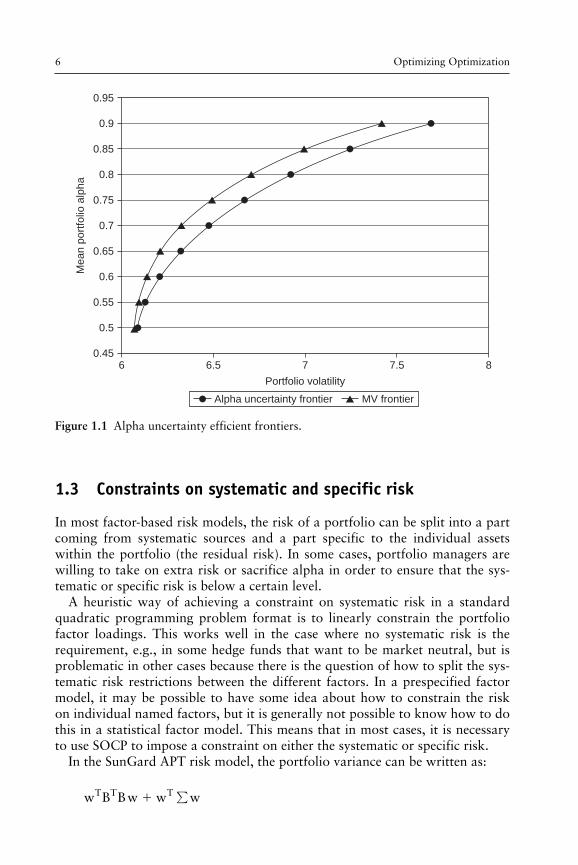
Figure 1.1 shows the standard mean – variance frontier and the frontier gen-erated including the alpha uncertainty term ( “ Alpha Uncertainty Frontier ” ). The example has a 500-asset universe and no benchmark and the mean port-folio alpha is constrained to various values between the mean portfolio alpha found for the minimum variance portfolio (assuming no alpha uncertainty) and 0.9. The size of the confidence region around the mean estimated alphas (i.e., the value of k ) is increased as the constraint on the mean portfolio alpha is increased. The covariance matrix of estimation errors Ω is assumed to be the individual volatilities of the assets calculated using a SunGard APT risk model. The portfolio variance is also calculated using a SunGard APT risk model.
Some extensions to this, e.g., the use of a benchmark and active portfolio return, are straightforward.
The key questions to making practical use of alpha uncertainty are the spec-ification of the covariance matrix of estimation errors Ω and the size of the confidence region around the mean estimated alphas (the value of k ). This will depend on the alpha generation process used by the practitioner and, as for the alpha generation process, it is suggested that backtesting be used to aid in the choice of appropriate covariance matrices Ω and confidence region sizes k . From a practical point of view, for reasonably sized problems, it is helpful if the covariance matrix Ω is either diagonal or a factor model is used.
06_P374952_Ch01.indd 506_P374952_Ch01.indd 5 9/15/2009 5:13:49 PM9/15/2009 5:13:49 PM
Optimizing Optimization6
1.3 Constraints on systematic and specific risk
In most factor-based risk models, the risk of a portfolio can be split into a part coming from systematic sources and a part specific to the individual assets within the portfolio (the residual risk). In some cases, portfolio managers are willing to take on extra risk or sacrifice alpha in order to ensure that the sys-tematic or specific risk is below a certain level.
A heuristic way of achieving a constraint on systematic risk in a standard quadratic programming problem format is to linearly constrain the portfolio factor loadings. This works well in the case where no systematic risk is the requirement, e.g., in some hedge funds that want to be market neutral, but is problematic in other cases because there is the question of how to split the sys-tematic risk restrictions between the different factors. In a prespecified factor model, it may be possible to have some idea about how to constrain the risk on individual named factors, but it is generally not possible to know how to do this in a statistical factor model. This means that in most cases, it is necessary to use SOCP to impose a constraint on either the systematic or specific risk.
In the SunGard APT risk model, the portfolio variance can be written as:
w B Bw w wT T T� ∑
0.75
0.7
0.65
0.6
0.55
0.5
0.456 6.5 7
Portfolio volatility
7.5 8
0.95
0.9
0.85
0.8
Mean p
ort
folio
alp
ha
Alpha uncertainty frontier MV frontier
Figure 1.1 Alpha uncertainty efficient frontiers.
06_P374952_Ch01.indd 606_P374952_Ch01.indd 6 9/15/2009 5:13:49 PM9/15/2009 5:13:49 PM
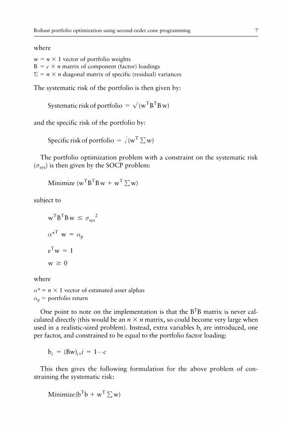
Robust portfolio optimization using second-order cone programming 7
where
w � n � 1 vector of portfolio weights B � c � n matrix of component (factor) loadings Σ � n � n diagonal matrix of specific (residual) variances
The systematic risk of the portfolio is then given by:
Systematic riskof por oliotf w B B wT T� √ ( )
and the specific risk of the portfolio by:
Specific riskof portfolio � � (w w)T ∑
The portfolio optimization problem with a constraint on the systematic risk ( σ sys ) is then given by the SOCP problem:
Minimize ( )w B Bw w wT T T� ∑
subject to
w B BwT T � σsys
2
α α* wT
p�
e w 1T �
w 0�
where
α * � n � 1 vector of estimated asset alphas α p � portfolio return
One point to note on the implementation is that the B T B matrix is never cal-culated directly (this would be an n � n matrix, so could become very large when used in a realistic-sized problem). Instead, extra variables b i are introduced, one per factor, and constrained to be equal to the portfolio factor loading:
b Bw 1i i c� �( ) , i ⋅⋅⋅
This then gives the following formulation for the above problem of con-straining the systematic risk:
Minimize( )b b w wT T� ∑
06_P374952_Ch01.indd 706_P374952_Ch01.indd 7 9/15/2009 5:13:50 PM9/15/2009 5:13:50 PM
Optimizing Optimization8
subject to
b bT � σsys
2
α α* wT
p�
e w 1T �
b B w�
w 0�
Similarly , the problem with a constraint on the specific risk ( σ spe ) is given by:
Minimize T( )b b w wT � ∑
subject to
w wT ∑ � σspe
2
α α* wT
p�
e w 1T �
b B w�
w 0�
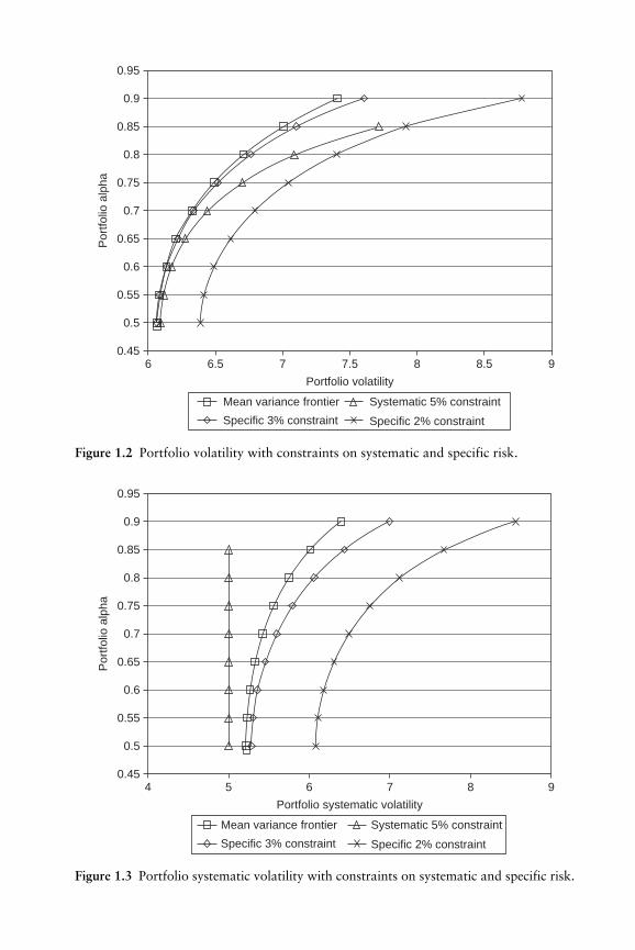
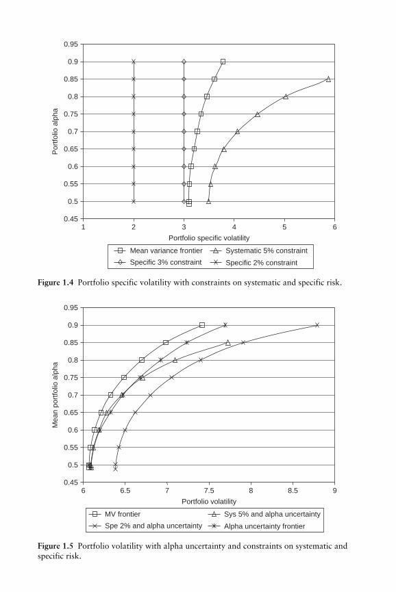
Figure 1.2 shows the standard mean – variance frontier and the frontiers gen-erated with constraints on the specific risk of 2% and 3%, and on the sys-tematic risk of 5%. The example has a 500-asset universe and no benchmark and the portfolio alpha is constrained to various values between the portfolio alpha found for the minimum variance portfolio and 0.9. (For the 5% con-straint on the systematic risk, it was not possible to find a feasible solution with a portfolio alpha of 0.9.) Figure 1.3 shows the systematic portfolio vola-tilities and Figure 1.4 shows the specific portfolio volatilities for the same set of optimizations.
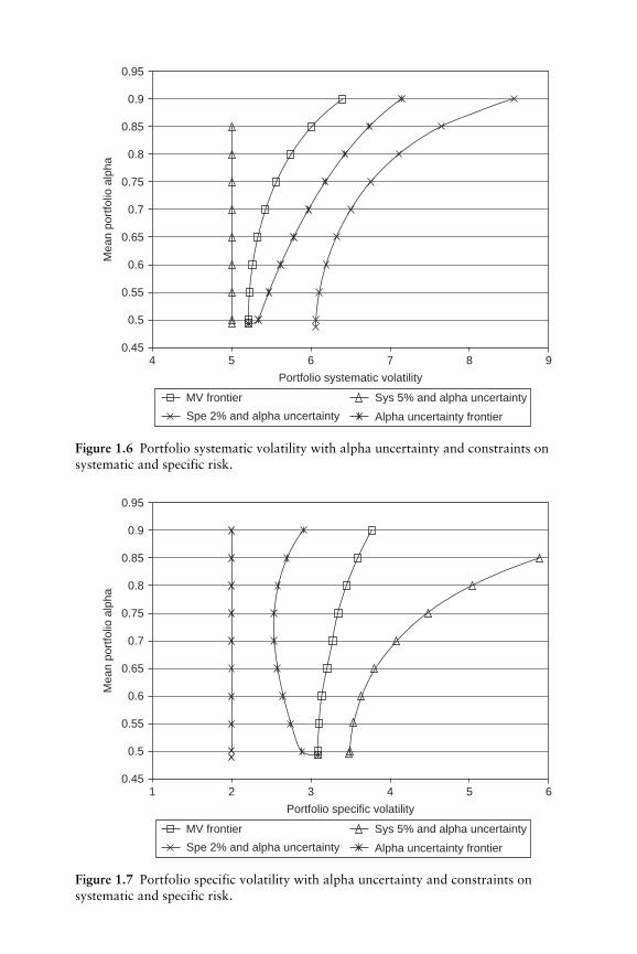
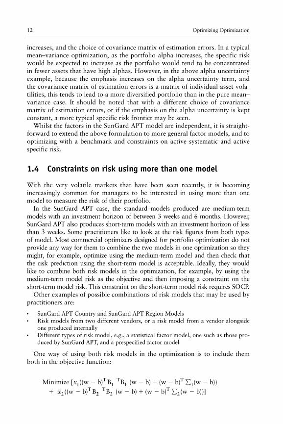
Constraints on systematic or specific volatility can be combined with the alpha uncertainty described in the previous section. The resulting frontiers can be seen in Figures 1.5 – 1.7 (the specific 3% constraint frontier is not shown because this coincides with the Alpha Uncertainty Frontier for all but the first point).
The shape of the specific risk frontier for the alpha uncertainty frontier (see Figure 1.7 ) is unusual. This is due to a combination of increasing the empha-sis on the alpha uncertainty as the constraint on the mean portfolio alpha
06_P374952_Ch01.indd 806_P374952_Ch01.indd 8 9/15/2009 5:13:50 PM9/15/2009 5:13:50 PM
0.75
0.7
0.65
0.6
0.55
0.5
0.456 6.5 7
Portfolio volatility
7.5 8 8.5 9
0.95
0.9
0.85
0.8
Port
folio
alp
ha
Specific 2% constraint
Mean variance frontier Systematic 5% constraint
Specific 3% constraint
Figure 1.2 Portfolio volatility with constraints on systematic and specific risk.
0.75
0.7
0.65
0.6
0.55
0.5
0.454 5 6
Portfolio systematic volatility
7 8 9
0.95
0.9
0.85
0.8
Port
folio
alp
ha
Specific 2% constraint
Mean variance frontier Systematic 5% constraint
Specific 3% constraint
Figure 1.3 Portfolio systematic volatility with constraints on systematic and specific risk.
06_P374952_Ch01.indd 906_P374952_Ch01.indd 9 9/15/2009 5:13:51 PM9/15/2009 5:13:51 PM
0.75
0.7
0.65
0.6
0.55
0.5
0.451 2 3
Portfolio specific volatility
4 5 6
0.95
0.9
0.85
0.8
Po
rtfo
lio a
lpha
Specific 2% constraint
Mean variance frontier Systematic 5% constraint
Specific 3% constraint
Figure 1.4 Portfolio specific volatility with constraints on systematic and specific risk.
0.75
0.7
0.65
0.6
0.55
0.5
0.456 6.5 7
Portfolio volatility
7.5 8 8.5 9
0.95
0.9
0.85
0.8
Mean p
ort
folio
alp
ha
Alpha uncertainty frontier
Sys 5% and alpha uncertaintyMV frontier
Spe 2% and alpha uncertainty
Figure 1.5 Portfolio volatility with alpha uncertainty and constraints on systematic and specific risk.
06_P374952_Ch01.indd 1006_P374952_Ch01.indd 10 9/15/2009 5:13:52 PM9/15/2009 5:13:52 PM
0.75
0.7
0.65
0.6
0.55
0.5
0.454 5 6
Portfolio systematic volatility
7 8 9
0.95
0.9
0.85
0.8
Me
an
po
rtfo
lio a
lph
a
Alpha uncertainty frontier
Sys 5% and alpha uncertaintyMV frontier
Spe 2% and alpha uncertainty
Figure 1.6 Portfolio systematic volatility with alpha uncertainty and constraints on systematic and specific risk.
0.75
0.7
0.65
0.6
0.55
0.5
0.451 2 3
Portfolio specific volatility
4 5 6
0.95
0.9
0.85
0.8
Me
an
po
rtfo
lio a
lph
a
Alpha uncertainty frontier
Sys 5% and alpha uncertaintyMV frontier
Spe 2% and alpha uncertainty
Figure 1.7 Portfolio specific volatility with alpha uncertainty and constraints on systematic and specific risk.
06_P374952_Ch01.indd 1106_P374952_Ch01.indd 11 9/15/2009 5:13:52 PM9/15/2009 5:13:52 PM
Optimizing Optimization12
increases, and the choice of covariance matrix of estimation errors. In a typical mean – variance optimization, as the portfolio alpha increases, the specific risk would be expected to increase as the portfolio would tend to be concentrated in fewer assets that have high alphas. However, in the above alpha uncertainty example, because the emphasis increases on the alpha uncertainty term, and the covariance matrix of estimation errors is a matrix of individual asset vola-tilities, this tends to lead to a more diversified portfolio than in the pure mean – variance case. It should be noted that with a different choice of covariance matrix of estimation errors, or if the emphasis on the alpha uncertainty is kept constant, a more typical specific risk frontier may be seen.
Whilst the factors in the SunGard APT model are independent, it is straight-forward to extend the above formulation to more general factor models, and to optimizing with a benchmark and constraints on active systematic and active specific risk.
1.4 Constraints on risk using more than one model
With the very volatile markets that have been seen recently, it is becoming increasingly common for managers to be interested in using more than one model to measure the risk of their portfolio.
In the SunGard APT case, the standard models produced are medium-term models with an investment horizon of between 3 weeks and 6 months. However, SunGard APT also produces short-term models with an investment horizon of less than 3 weeks. Some practitioners like to look at the risk figures from both types of model. Most commercial optimizers designed for portfolio optimization do not provide any way for them to combine the two models in one optimization so they might, for example, optimize using the medium-term model and then check that the risk prediction using the short-term model is acceptable. Ideally, they would like to combine both risk models in the optimization, for example, by using the medium-term model risk as the objective and then imposing a constraint on the short-term model risk. This constraint on the short-term model risk requires SOCP.
Other examples of possible combinations of risk models that may be used by practitioners are:
● SunGard APT Country and SunGard APT Region Models ● Risk models from two different vendors, or a risk model from a vendor alongside
one produced internally ● Different types of risk model, e.g., a statistical factor model, one such as those pro-
duced by SunGard APT, and a prespecified factor model
One way of using both risk models in the optimization is to include them both in the objective function:
Minimize
[ (( ) ( ) ( ) ( ))(( )
x
x1 1 1 1
2
w b B B w b w b w bw b B
� � � � �
� �
T T T
T∑
22 2 2 T TB w b w b w b( ) ( ) ( ))]� � � �∑
06_P374952_Ch01.indd 1206_P374952_Ch01.indd 12 9/15/2009 5:13:53 PM9/15/2009 5:13:53 PM
Robust portfolio optimization using second-order cone programming 13
subject to
α α* wT
p�
e w 1T �
w w� max
w 0�
where
w � n � 1 vector of portfolio weights
b � n � 1 vector of benchmark weights
B i � c � n matrix of component (factor) loadings for risk model i
Σ i � n � n diagonal matrix of specific (residual) variances for risk model i
x i � weight of risk model i in objective function ( x i � 0)
α * � n � 1 vector of estimated asset alphas
α p � portfolio return
w max � n � 1 vector of maximum asset weights in the portfolio
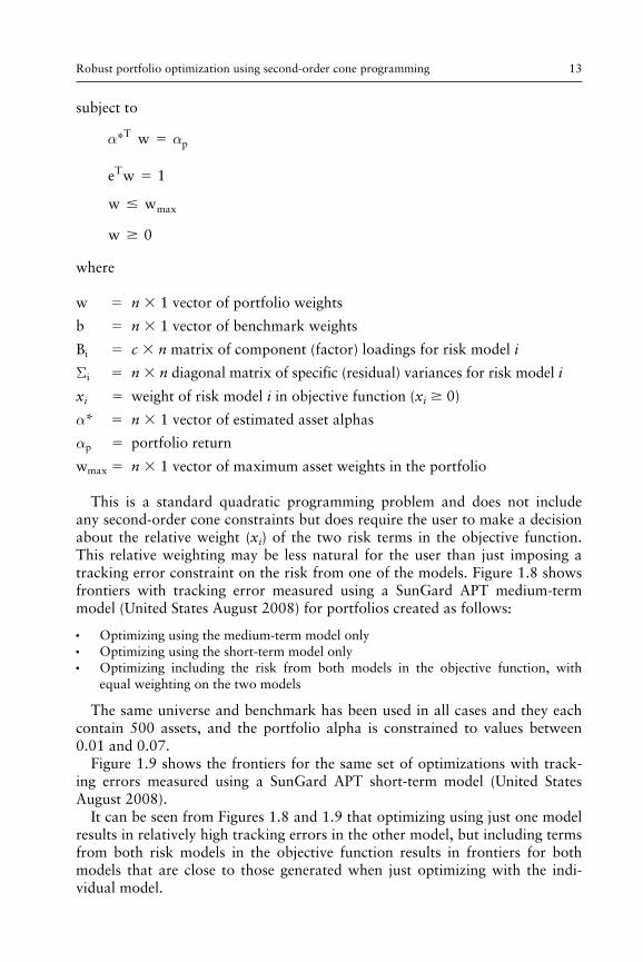
This is a standard quadratic programming problem and does not include any second-order cone constraints but does require the user to make a decision about the relative weight ( x i ) of the two risk terms in the objective function. This relative weighting may be less natural for the user than just imposing a tracking error constraint on the risk from one of the models. Figure 1.8 shows frontiers with tracking error measured using a SunGard APT medium-term model (United States August 2008) for portfolios created as follows:
● Optimizing using the medium-term model only ● Optimizing using the short-term model only ● Optimizing including the risk from both models in the objective function, with
equal weighting on the two models
The same universe and benchmark has been used in all cases and they each contain 500 assets, and the portfolio alpha is constrained to values between 0.01 and 0.07.
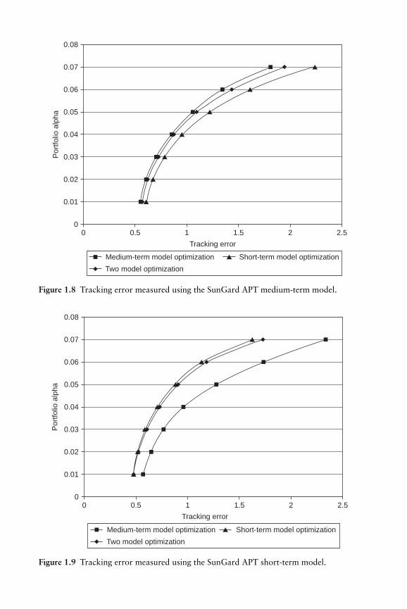
Figure 1.9 shows the frontiers for the same set of optimizations with track-ing errors measured using a SunGard APT short-term model (United States August 2008).
It can be seen from Figures 1.8 and 1.9 that optimizing using just one model results in relatively high tracking errors in the other model, but including terms from both risk models in the objective function results in frontiers for both models that are close to those generated when just optimizing with the indi-vidual model.
06_P374952_Ch01.indd 1306_P374952_Ch01.indd 13 9/15/2009 5:13:53 PM9/15/2009 5:13:53 PM
0
0.01
0.02
0.03
0.04
0.05
0.06
0.07
0 0.5 1
Tracking error
1.5 2 2.5
0.08
Port
folio
alp
ha
Short-term model optimizationMedium-term model optimization
Two model optimization
Figure 1.8 Tracking error measured using the SunGard APT medium-term model.
0
0.01
0.02
0.03
0.04
0.05
0.06
0.07
0 0.5 1
Tracking error
1.5 2 2.5
0.08
Port
folio
alp
ha
Short-term model optimizationMedium-term model optimization
Two model optimization
Figure 1.9 Tracking error measured using the SunGard APT short-term model.
06_P374952_Ch01.indd 1406_P374952_Ch01.indd 14 9/15/2009 5:13:53 PM9/15/2009 5:13:53 PM
Robust portfolio optimization using second-order cone programming 15
Using SOCP, it is possible to include both risk models in the optimization by including the risk term from one in the objective function and constraining on the risk term from the other model:
Minimize [( ) ( ) ( ) ( )]w b B B w b w b w bT T1
T� � � � �1 1∑
subject to
( ) ( ) ( ) ( )w b B B w b w b w bT T T� � � � � �2 2 2 22∑ σa
α α* wT
p�
e w 1T �
w w� max
w 0�
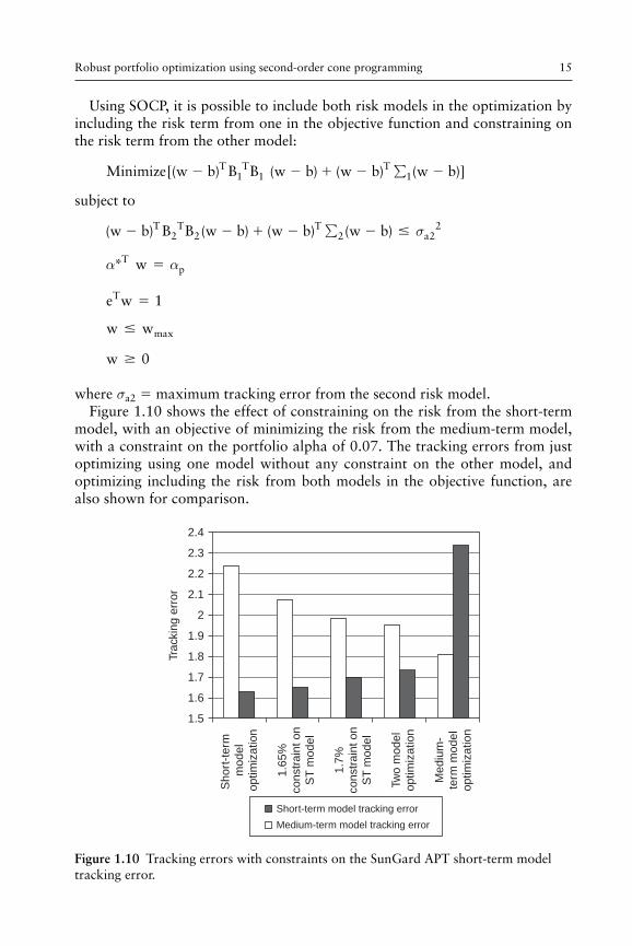
where σ a2 � maximum tracking error from the second risk model. Figure 1.10 shows the effect of constraining on the risk from the short-term
model, with an objective of minimizing the risk from the medium-term model, with a constraint on the portfolio alpha of 0.07. The tracking errors from just optimizing using one model without any constraint on the other model, and optimizing including the risk from both models in the objective function, are also shown for comparison.
1.5
1.6
1.7
1.8
1.9
2
2.1
2.2
2.3
2.4
Short
-term
model
optim
ization
1.6
5%
constr
ain
t on
ST
model
Mediu
m-
term
model
optim
ization
Tw
o m
odel
optim
ization
1.7
%
constr
ain
t on
ST
model
Tra
ckin
g e
rror
Short-term model tracking error
Medium-term model tracking error
Figure 1.10 Tracking errors with constraints on the SunGard APT short-term model tracking error.
06_P374952_Ch01.indd 1506_P374952_Ch01.indd 15 9/15/2009 5:13:54 PM9/15/2009 5:13:54 PM
Optimizing Optimization16
Whilst the discussion here has concerned using two SunGard APT risk mod-els, it should be noted that it is trivial to extend the above to any number of risk models, and to more general risk factor models.
1.5 Combining different risk measures
In some cases, it may be desirable to optimize using one risk measure for the objective and to constrain on some other risk measures. For example, the objective might be to minimize tracking error against a benchmark whilst con-straining the portfolio volatility. Another example could be where a pension fund manager or an institutional asset manager has an objective of minimizing tracking error against a market index, but also needs to constrain the tracking error against some internal model portfolio.
This can be achieved in a standard quadratic programming problem format by including both risk measures in the objective function and varying the rela-tive emphasis on them until a solution satisfying the risk constraint is found. The main disadvantage of this is that it is time consuming to find a solution and is difficult to extend to the case where there is to be a constraint on more than one additional risk measure. A quicker, more general approach is to use SOCP to implement constraints on the risk measures.
The first case, minimizing tracking error, whilst constraining portfolio vola-tility, results in the following SOCP problem when using the SunGard APT risk model:
Minimize ( )[ ( ) ( ) ( )]w b B B w b w b w bT T T� � � � �∑
subject to
α α* wT
p�
w B Bw w wT T T� �∑ σ2
e w 1T �
w w� max
w 0�
where
w � n � 1 vector of portfolio weights
b � n � 1 vector of benchmark weights
B � c � n matrix of component (factor) loadings
Σ � n � n diagonal matrix of specific (residual) variances
06_P374952_Ch01.indd 1606_P374952_Ch01.indd 16 9/15/2009 5:13:55 PM9/15/2009 5:13:55 PM
Robust portfolio optimization using second-order cone programming 17
σ � maximum portfolio volatility
α * � n � 1 vector of estimated asset alphas
α p � Portfolio return
w max � n � 1 vector of maximum asset weights in the portfolio
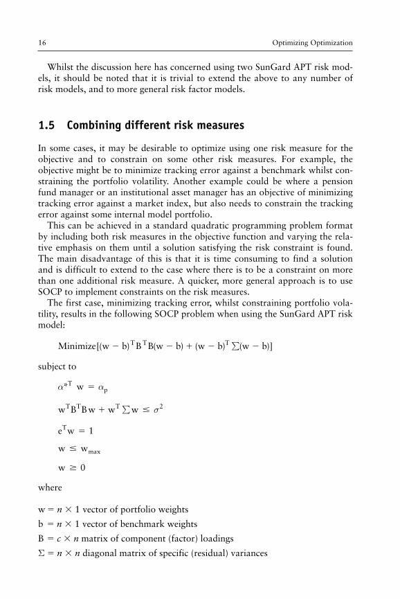
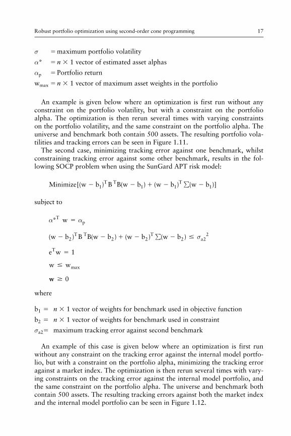
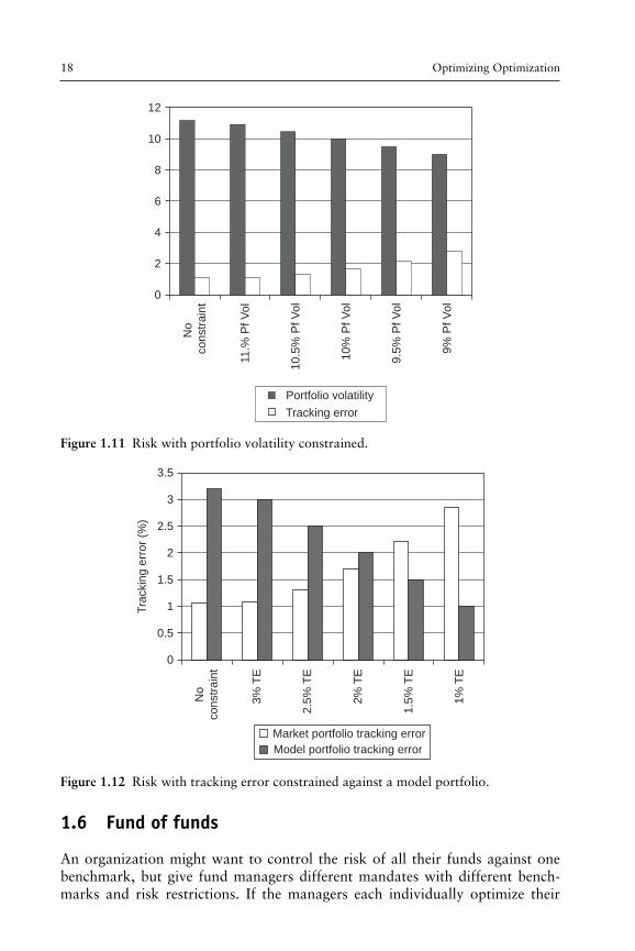
An example is given below where an optimization is first run without any constraint on the portfolio volatility, but with a constraint on the portfolio alpha. The optimization is then rerun several times with varying constraints on the portfolio volatility, and the same constraint on the portfolio alpha. The universe and benchmark both contain 500 assets. The resulting portfolio vola-tilities and tracking errors can be seen in Figure 1.11 .
The second case, minimizing tracking error against one benchmark, whilst constraining tracking error against some other benchmark, results in the fol-lowing SOCP problem when using the SunGard APT risk model:
Minimize[( ) ( ) ( ) ( )]w b B B w b w b w b1T T T� � � � �1 1 1∑
subject to
α α* wT
p�
( ) ( ) ( ) ( )w b B B w b w b w bT T T� � � � � �2 2 2 2 22∑ σa
e w 1T �
w w� max
w � 0
where
b 1 � n � 1 vector of weights for benchmark used in objective function
b 2 � n � 1 vector of weights for benchmark used in constraint
σ a2 � maximum tracking error against second benchmark
An example of this case is given below where an optimization is first run without any constraint on the tracking error against the internal model portfo-lio, but with a constraint on the portfolio alpha, minimizing the tracking error against a market index. The optimization is then rerun several times with vary-ing constraints on the tracking error against the internal model portfolio, and the same constraint on the portfolio alpha. The universe and benchmark both contain 500 assets. The resulting tracking errors against both the market index and the internal model portfolio can be seen in Figure 1.12 .
06_P374952_Ch01.indd 1706_P374952_Ch01.indd 17 9/15/2009 5:13:55 PM9/15/2009 5:13:55 PM
Optimizing Optimization18
1.6 Fund of funds
An organization might want to control the risk of all their funds against one benchmark, but give fund managers different mandates with different bench-marks and risk restrictions. If the managers each individually optimize their
0
2
4
6
8
10
12
No
constr
ain
t
11.%
Pf V
ol
10.5
% P
f V
ol
10%
Pf V
ol
9.5
% P
f V
ol
9%
Pf V
ol
Portfolio volatility
Tracking error
Figure 1.11 Risk with portfolio volatility constrained.
3.5
2.5
3
1.5
0.5
0
No
constr
ain
t
Tra
ckin
g e
rror
(%)
3%
TE
2.5
% T
E
2%
TE
1.5
% T
E
1%
TE
1
2
Market portfolio tracking error
Model portfolio tracking error
Figure 1.12 Risk with tracking error constrained against a model portfolio.
06_P374952_Ch01.indd 1806_P374952_Ch01.indd 18 9/15/2009 5:13:55 PM9/15/2009 5:13:55 PM
Robust portfolio optimization using second-order cone programming 19
own fund against their own benchmark, then it can be difficult to control the overall risk for the organization. From the overall management point of view, it would be better if the funds could be optimized together, taking into account the overall benchmark. One way to do this is to use SOCP to impose the track-ing error constraints on the individual funds, and optimize with an objective of minimizing the tracking error of the combined funds against the overall bench-mark, with constraints on the minimum alpha for each of the funds. Using the SunGard APT risk model, this results in the following SOCP problem:
Minimize ( ) ( ) ( ) ( )w b B B w b w b w bc cT T
c c c cT
c c� � � � �∑
subject to
w w , 1c i� � �∑ ∑i i i if f fi , 0
( ) ( ) ( ) ( ) ,w b B B w b w b w b 1i iT T
i i i iT
i i� � � � � � �∑ ⋅⋅⋅σai i m2
e w 1,Ti � �i m1⋅⋅⋅
w w maxi i i� � �0 1, , i m⋅⋅⋅
α*i p
Tiw 1� �α i i m, ⋅⋅⋅
where
m � number of funds
w i � n � 1 vector of portfolio weights for fund i
b i � n � 1 vector of benchmark weights for fund i
w c � n � 1 vector of weights for overall (combined) portfolio
f i � weight of fund i in overall (combined) portfolio
b c � n � 1 vector of overall benchmark weights
B � c � n matrix of component (factor) loadings
Σ � n � n diagonal matrix of specific (residual) variances
σ a i � maximum tracking error for fund i
max i � n � 1 vector of maximum weights for fund i
α*i � n � 1 vector of assets alphas for fund i
α p i � minimum portfolio alpha for fund i
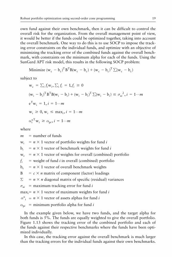
In the example given below, we have two funds, and the target alpha for both funds is 5%. The funds are equally weighted to give the overall portfolio. Figure 1.13 shows the tracking error of the combined portfolio and each of the funds against their respective benchmarks where the funds have been opti-mized individually.
In this case, the tracking error against the overall benchmark is much larger than the tracking errors for the individual funds against their own benchmarks.
06_P374952_Ch01.indd 1906_P374952_Ch01.indd 19 9/15/2009 5:13:57 PM9/15/2009 5:13:57 PM
Optimizing Optimization20
This sort of situation would arise when the overall benchmark and the indi-vidual fund benchmarks are very different, e.g., in the case where the overall benchmark is a market index and the individual funds are a sector fund and a value fund. It is unlikely to occur when both the overall and individual fund benchmarks are very similar, for instance, when they are all market indexes.
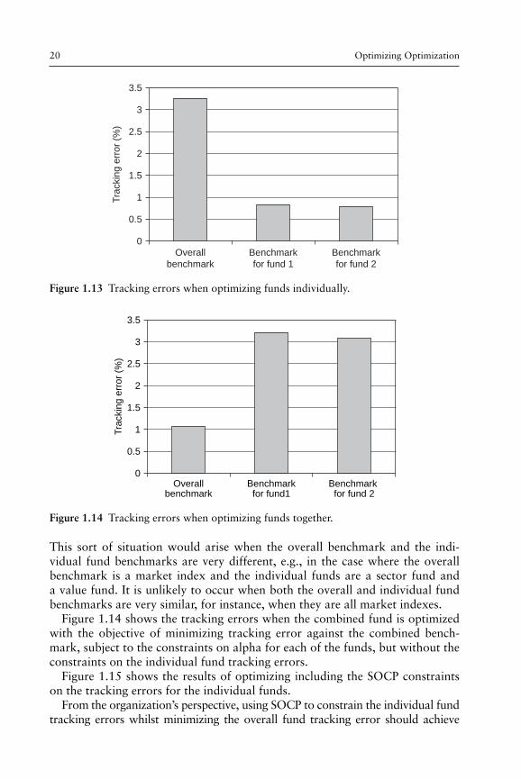
Figure 1.14 shows the tracking errors when the combined fund is optimized with the objective of minimizing tracking error against the combined bench-mark, subject to the constraints on alpha for each of the funds, but without the constraints on the individual fund tracking errors.
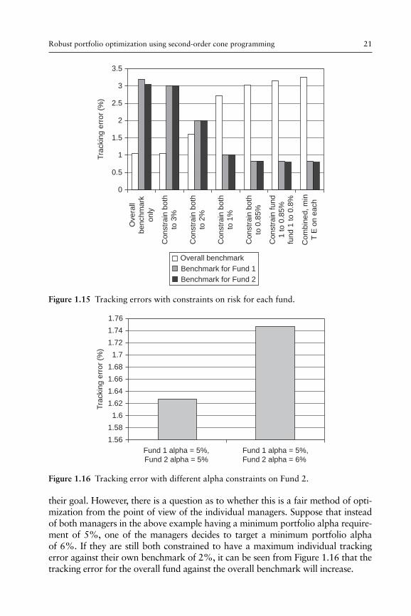
Figure 1.15 shows the results of optimizing including the SOCP constraints on the tracking errors for the individual funds.
From the organization’s perspective, using SOCP to constrain the individual fund tracking errors whilst minimizing the overall fund tracking error should achieve
Overall
benchmark
Tra
ckin
g e
rror
(%)
3.5
3
2.5
2
1.5
1
0.5
0
Benchmark
for fund 1
Benchmark
for fund 2
Figure 1.13 Tracking errors when optimizing funds individually.
Overallbenchmark
Tra
ckin
g e
rror
(%)
3.5
3
2.5
2
1.5
1
0.5
0Benchmarkfor fund1
Benchmark for fund 2
Figure 1.14 Tracking errors when optimizing funds together.
06_P374952_Ch01.indd 2006_P374952_Ch01.indd 20 9/15/2009 5:13:57 PM9/15/2009 5:13:57 PM
Robust portfolio optimization using second-order cone programming 21
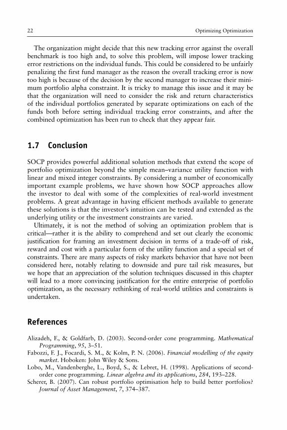
their goal. However, there is a question as to whether this is a fair method of opti-mization from the point of view of the individual managers. Suppose that instead of both managers in the above example having a minimum portfolio alpha require-ment of 5%, one of the managers decides to target a minimum portfolio alpha of 6%. If they are still both constrained to have a maximum individual tracking error against their own benchmark of 2%, it can be seen from Figure 1.16 that the tracking error for the overall fund against the overall benchmark will increase.
2.5
3
3.5
1.5
0.5
0
Overa
ll
be
nch
ma
rk
on
ly
Tra
ckin
g e
rror
(%)
Co
nstr
ain
bo
th
to 3
%
Co
nstr
ain
bo
th
to 2
%
Co
nstr
ain
bo
th
to 1
%
Co
nstr
ain
bo
th
to 0
.85%
Co
nstr
ain
fu
nd
1 to 0
.85%
fund 1
to 0
.8%
Com
bin
ed, m
in
T E
on e
ach
1
2
Benchmark for Fund 1
Benchmark for Fund 2
Overall benchmark
Figure 1.15 Tracking errors with constraints on risk for each fund.
Fund 1 alpha = 5%,
Fund 2 alpha = 5%
Fund 1 alpha = 5%,
Fund 2 alpha = 6%
Tra
ckin
g e
rror
(%)
1.76
1.74
1.72
1.7
1.68
1.66
1.64
1.62
1.6
1.58
1.56
Figure 1.16 Tracking error with different alpha constraints on Fund 2.
06_P374952_Ch01.indd 2106_P374952_Ch01.indd 21 9/15/2009 5:13:58 PM9/15/2009 5:13:58 PM
Optimizing Optimization22
The organization might decide that this new tracking error against the overall benchmark is too high and, to solve this problem, will impose lower tracking error restrictions on the individual funds. This could be considered to be unfairly penalizing the first fund manager as the reason the overall tracking error is now too high is because of the decision by the second manager to increase their mini-mum portfolio alpha constraint. It is tricky to manage this issue and it may be that the organization will need to consider the risk and return characteristics of the individual portfolios generated by separate optimizations on each of the funds both before setting individual tracking error constraints, and after the combined optimization has been run to check that they appear fair.
1.7 Conclusion
SOCP provides powerful additional solution methods that extend the scope of portfolio optimization beyond the simple mean – variance utility function with linear and mixed integer constraints. By considering a number of economically important example problems, we have shown how SOCP approaches allow the investor to deal with some of the complexities of real-world investment problems. A great advantage in having efficient methods available to generate these solutions is that the investor’s intuition can be tested and extended as the underlying utility or the investment constraints are varied.
Ultimately , it is not the method of solving an optimization problem that is critical — rather it is the ability to comprehend and set out clearly the economic justification for framing an investment decision in terms of a trade-off of risk, reward and cost with a particular form of the utility function and a special set of constraints. There are many aspects of risky markets behavior that have not been considered here, notably relating to downside and pure tail risk measures, but we hope that an appreciation of the solution techniques discussed in this chapter will lead to a more convincing justification for the entire enterprise of portfolio optimization, as the necessary rethinking of real-world utilities and constraints is undertaken.
References
Alizadeh , F. , & Goldfarb , D. ( 2003 ) . Second-order cone programming . Mathematical Programming , 95 , 3 – 51 .
Fabozzi , F. J. , Focardi , S. M. , & Kolm , P. N. ( 2006 ) . Financial modelling of the equity market . Hoboken : John Wiley & Sons .
Lobo , M. , Vandenberghe , L. , Boyd , S. , & Lebret , H. ( 1998 ) . Applications of second-order cone programming . Linear algebra and its applications , 284 , 193 – 228 .
Scherer , B. ( 2007 ) . Can robust portfolio optimisation help to build better portfolios? Journal of Asset Management , 7 , 374 – 387 .
06_P374952_Ch01.indd 2206_P374952_Ch01.indd 22 9/15/2009 5:13:59 PM9/15/2009 5:13:59 PM