1

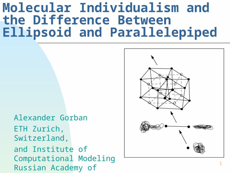
The Kinetic Basis of Molecular Individualism and the Difference Between Ellipsoid and Parallelepiped

Alexander Gorban

ETH Zurich, Switzerland,

and Institute of Computational Modeling Russian Academy of Sciences

2

3

The Kinetic Basis of Molecular Individualism and the Difference Between Ellipsoid and Parallelepiped

Alexander Gorban

ETH Zurich, Switzerland,

and Institute of Computational Modeling Russian Academy of Sciences

4

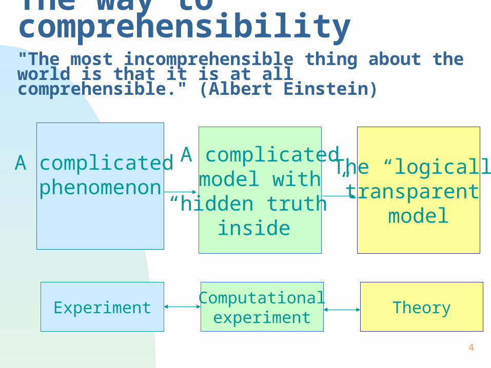
The way to comprehensibility"The most incomprehensible thing about the world is that it is at all comprehensible." (Albert Einstein)

A complicated phenomenon

A complicatedmodel with

“hidden truth” inside

The “logicallytransparent”

model

ExperimentComputational

experimentTheory

5

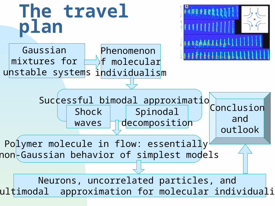
The travel plan

Gaussian mixtures for

unstable systems

Phenomenon of molecular individualism

Successful bimodal approximationsShockwaves

Spinodaldecomposition

Polymer molecule in flow: essentially non-Gaussian behavior of simplest models

Neurons, uncorrelated particles, and multimodal approximation for molecular individualism

Conclusion and

outlook

6

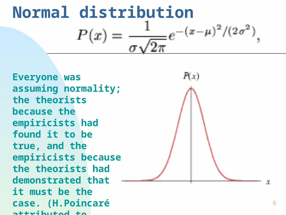
Normal distribution

Everyone was assuming normality; the theorists because the empiricists had found it to be true, and the empiricists because the theorists had demonstrated that it must be the case. (H.Poincaré attributed to Lippmann)

7

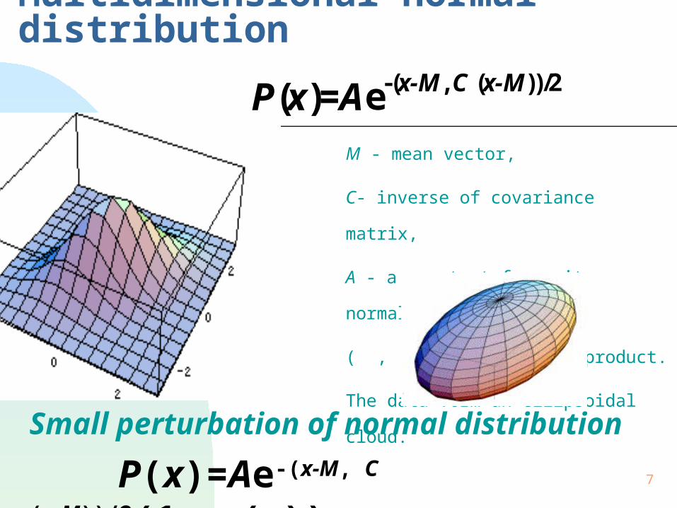
Multidimensional normal distribution

M - mean vector,

C- inverse of covariance matrix,

A - a constant for unit normalisation,

( , ) - usual scalar product.

The data form an ellipsoidal cloud.

P(x)=Ae-(x-M, C (x-M))/2

Small perturbation of normal distribution

P(x)=Ae-(x-M, C (x-M))/2(1+(x))

8

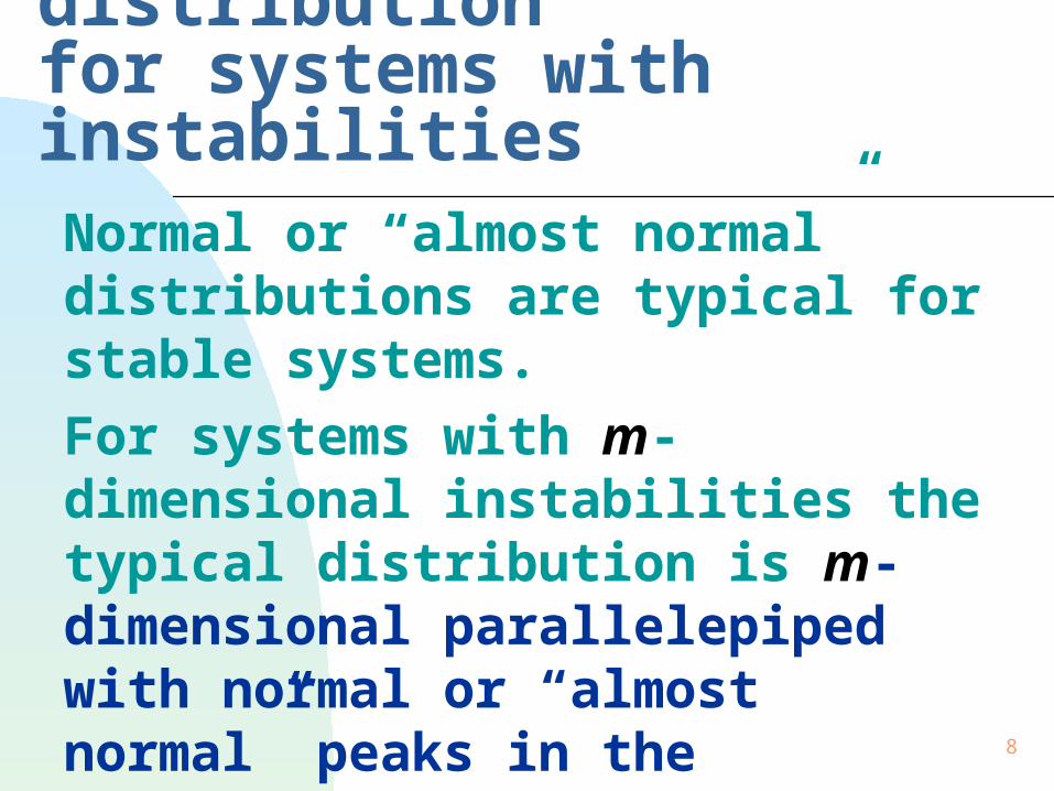
Typical multimodal distribution for systems with instabilitiesNormal or “almost normal” distributions are typical for stable systems.

For systems with m-dimensional instabilities the typical distribution is m-dimensional parallelepiped with normal or “almost normal” peaks in the vertices.

9

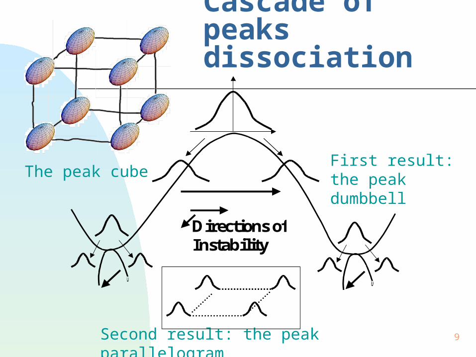
Cascade of peaks dissociation

Second result: the peak parallelogram

The peak cube

Directions ofInstability

First result: the peak dumbbell

10

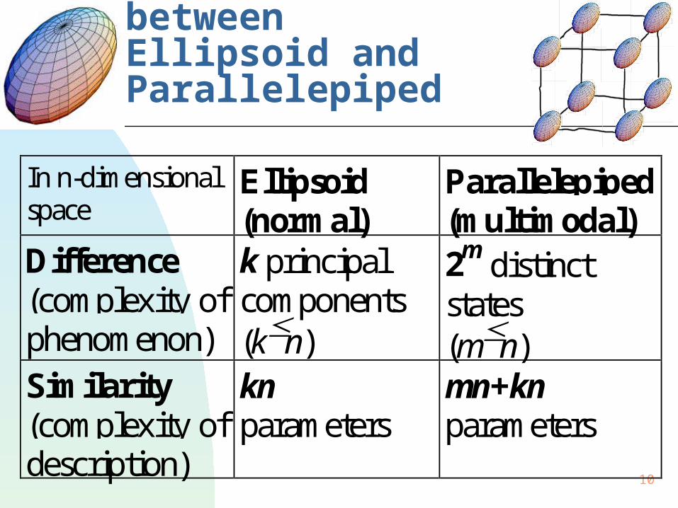
The similarity and the difference between Ellipsoid and Parallelepiped

In n-dimensionalspace

Ellipsoid(normal)

Parallelepiped(multimodal)

Difference(complexity ofphenomenon)

k principalcomponents(kn)

2m distinctstates(mn)

Similarity(complexity ofdescription)

knparameters

mn+knparameters

11

What is the complexity of a parallelepiped?The way from edges to vertices is easy. But is it easy to go back, from vertexes to edges?

The problem:

Let us have a finite set S in Rn. Suppose it is a sufficiently big set of some of vertices of an unknown parallelepiped with unknown dimension, mn, S2m.

Please find the edges of this parallelepiped.

What is the complexity of this problem?

12

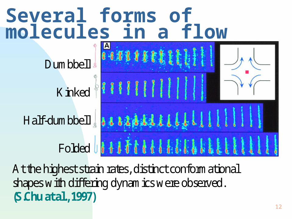
Several forms of molecules in a flow

Dumbbell

Kinked

Half-dumbbell

Folded

At the highest strain rates, distinct conformationalshapes with differing dynamics were observed.(S.Chu at al., 1997)

13

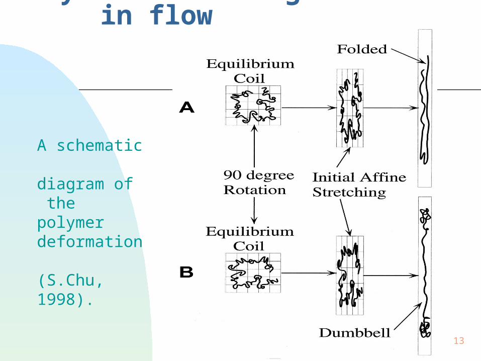
Polymer stretching in flow

A schematic diagram of the polymer deformation (S.Chu, 1998).

14

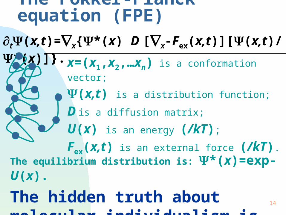
The Fokker-Planck equation (FPE)t(x,t)=x{*(x) D [x-Fex(x,t)][(x,t)/ *(x)]}.

x=(x1,x2,…xn) is a conformation vector;

(x,t) is a distribution function;

D is a diffusion matrix;

U(x) is an energy (/kT);

Fex(x,t) is an external force (/kT).

The equilibrium distribution is: *(x)=exp-U(x).

The hidden truth about molecular individualism is inside the FPE

15

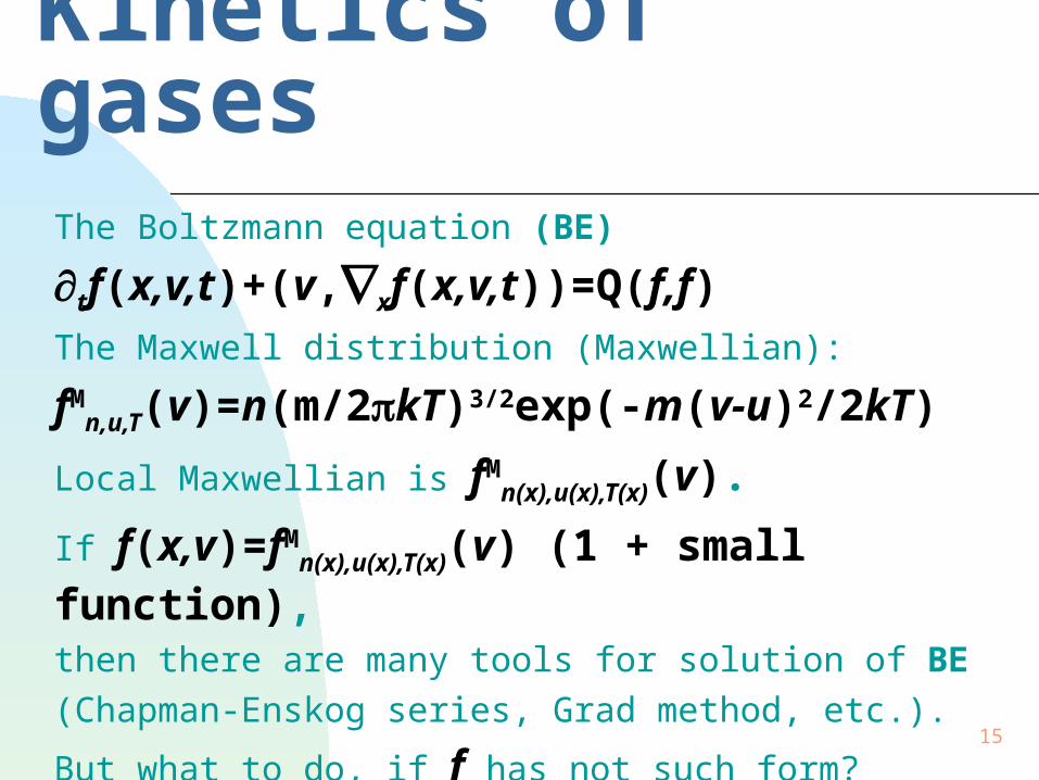
Kinetics of gasesThe Boltzmann equation (BE)

tf(x,v,t)+(v,xf(x,v,t))=Q(f,f)The Maxwell distribution (Maxwellian):

fMn,u,T(v)=n(m/2kT)3/2exp(-m(v-u)2/2kT)

Local Maxwellian is fMn(x),u(x),T(x)(v).

If f(x,v)=fMn(x),u(x),T(x)(v) (1 + small function),

then there are many tools for solution of BE

(Chapman-Enskog series, Grad method, etc.).

But what to do, if f has not such form?

16

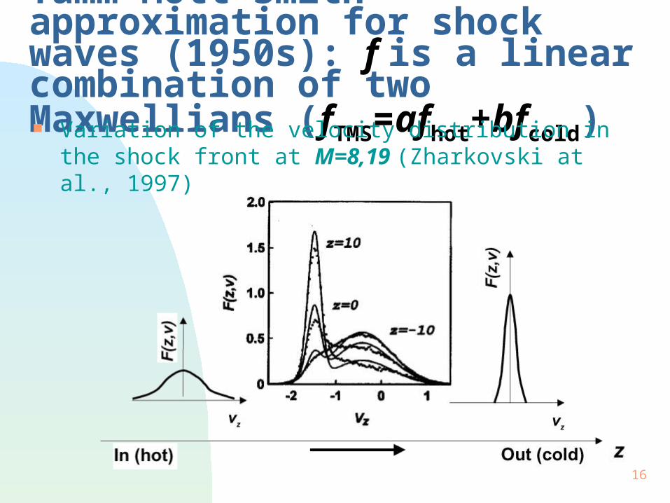
Tamm-Mott-Smith approximation for shock waves (1950s): f is a linear combination of two Maxwellians (fTMS=afhot+bfcold) Variation of the velocity distribution in the shock front at

M=8,19 (Zharkovski at al., 1997)

17

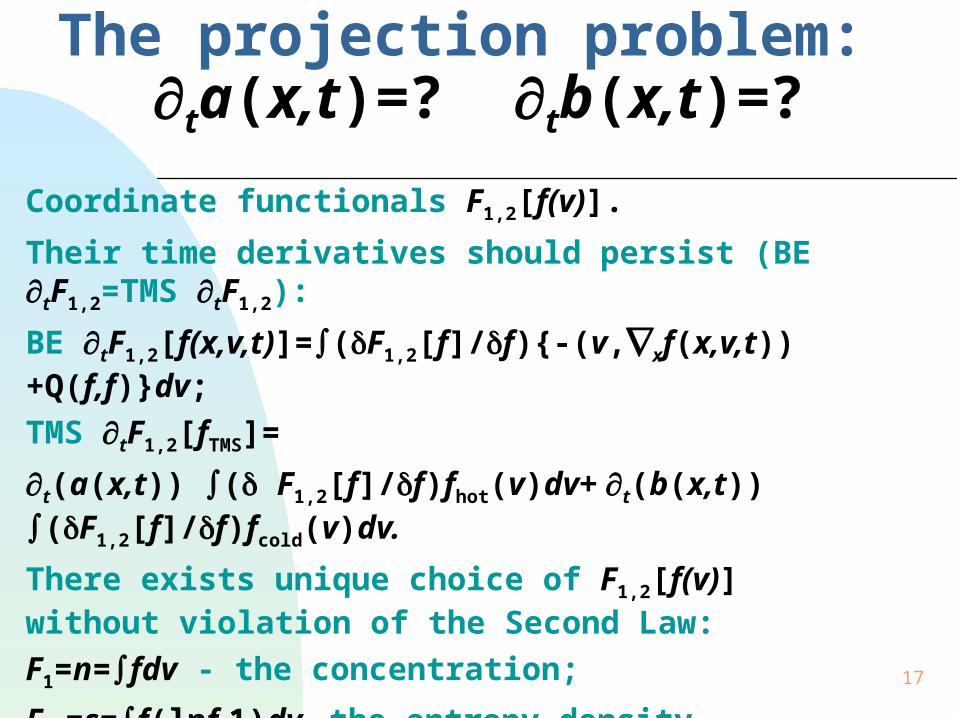
The projection problem: ta(x,t)=? tb(x,t)=?

Coordinate functionals F1,2[f(v)].

Their time derivatives should persist (BE tF1,2=TMS tF1,2):

BE tF1,2[f(x,v,t)]=(F1,2[f]/f){-(v,xf(x,v,t))+Q(f,f)}dv;

TMS tF1,2[fTMS]=

t(a(x,t)) ( F1,2[f]/f)fhot(v)dv+ t(b(x,t)) (F1,2[f]/f)fcold(v)dv.

There exists unique choice of F1,2[f(v)]without violation of the Second Law:

F1=n=fdv - the concentration;

F2 =s=f(lnf-1)dv - the entropy density.

Proposed by M. Lampis (1977).

Uniqueness was proved by A. Gorban & I. Karlin (1990).

18

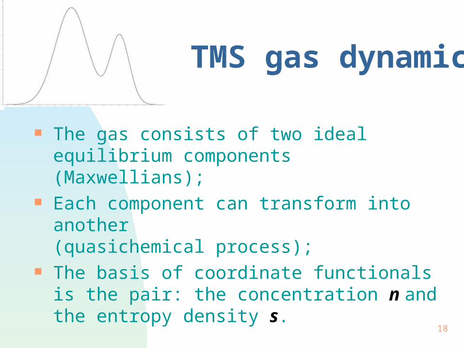
TMS gas dynamics

The gas consists of two ideal equilibrium components (Maxwellians);

Each component can transform into another (quasichemical process);

The basis of coordinate functionals is the pair: the concentration n and the entropy density s.

19

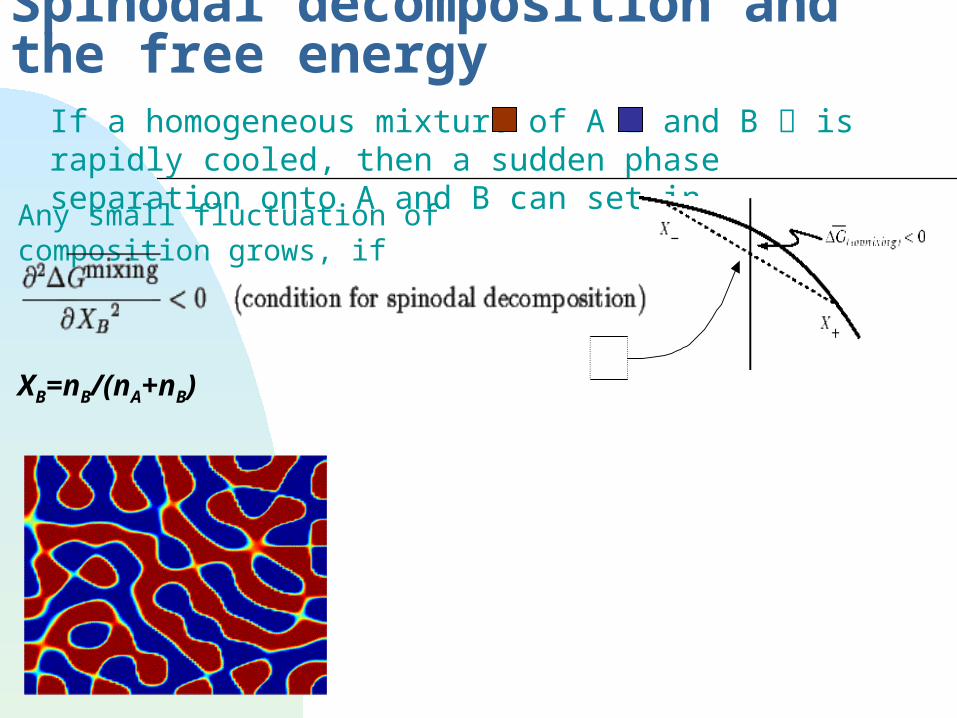
Spinodal decomposition and the free energyIf a homogeneous mixture of A and B is rapidly cooled, then a sudden phase separation onto A and B can set in.

Any small fluctuation of composition grows, if

XB=nB/(nA+nB)

20

Kinetic description of spinodal decomposition

Ginzburg-Landau free energy G=[(g(u(x))+1/2K(u(x))2]dx,where u(x)=XB(x)-XB;

Infinite-dimensional Fokker-Planck equation for distribution of fields u(x);

Perturbation theory expansions, or direct simulation, or…?

Model reduction: we do not need the whole distribution of fields u(x), but how to construct the appropriate variables?

21

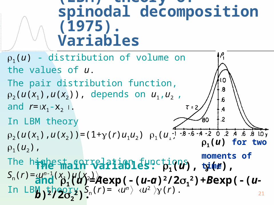
Langer- Bar-on- Miller (LBM) theory of spinodal decomposition (1975).Variables

1(u) - distribution of volume on the values of u.

The pair distribution function, 2(u(x1),u(x2)), depends on u1,u2 , and r=x1-x2 .

In LBM theory

2(u(x1),u(x2))=(1+(r)u1u2) 1(u1) 1(u2),

The highest correlation functions

Sn(r)=un-1(x1)u(x2),

In LBM theory Sn(r)= un u2 (r).The main variables: 1(u), (r), and 1(u)=Aexp(-(u-a)2/21

2)+Bexp(-(u-b)2/222).

LMB project FPE on (r) and this 1(u).

1(u) for two

moments of time

22

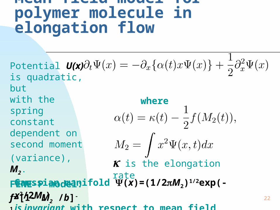
Mean field model for polymer molecule in elongation flow

where

Potential U(x) is quadratic, but with the spring constant dependent on second moment

(variance), M2.

FENE-P model:

f=[1- M2 /b]-1.

Gaussian manifold (x)=(1/2M2)1/2exp(-x2/2M2) is invariant with respect to mean field models

is the elongation rate

23

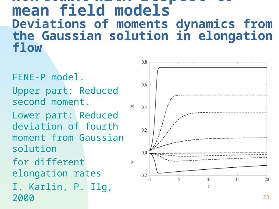
Gaussian manifold may be non-stable with respect to mean field modelsDeviations of moments dynamics from the Gaussian solution in elongation flow

FENE-P model.

Upper part: Reduced second moment.

Lower part: Reduced deviation of fourth moment from Gaussian solution

for different elongation rates

I. Karlin, P. Ilg, 2000

24

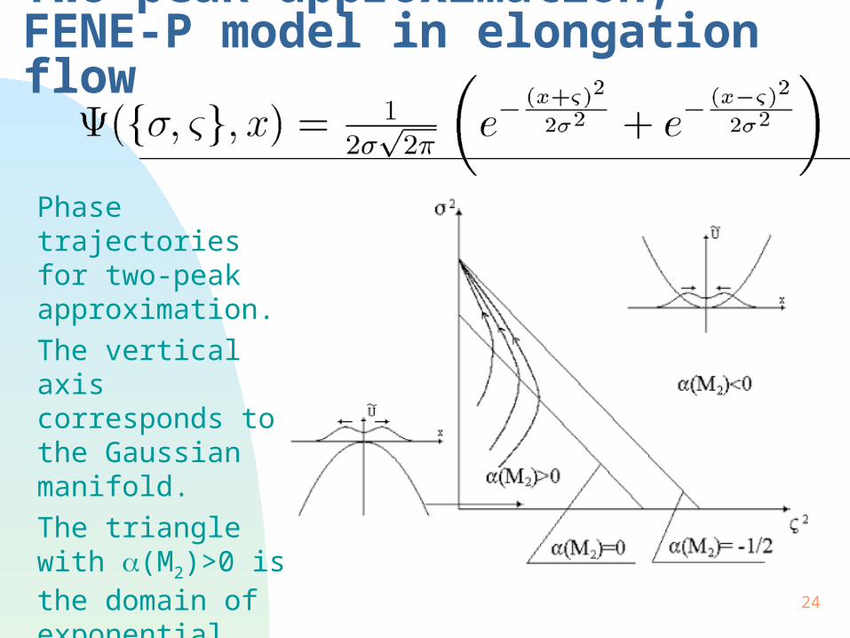
Two-peak approximation, FENE-P model in elongation flow

Phase trajectories for two-peak approximation.

The vertical axis corresponds to the Gaussian manifold.

The triangle with (M2)>0 is the domain of exponential instability.

25

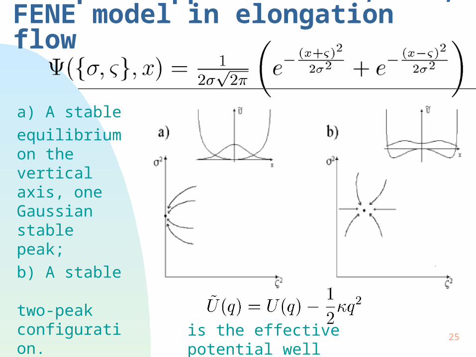
Two-peak approximation, FPE, FENE model in elongation flow

a) A stable

equilibrium on the vertical axis, one Gaussian stable peak;

b) A stable two-peak configuration.

Fokker-Planck equation.

is the effective potential well

26

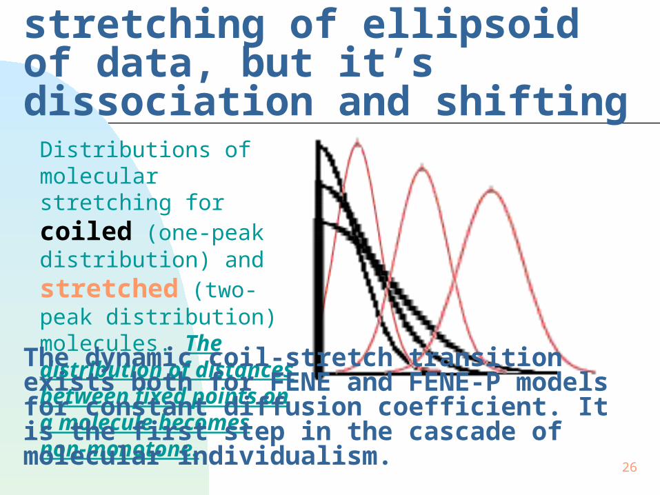
Dynamic coil-stretch transition is not a stretching of ellipsoid of data, but it’s dissociation and shifting

Distributions of molecular stretching for coiled (one-peak distribution) and stretched (two-peak distribution) molecules. The distribution of distances between fixed points on a molecule becomes non-monotone.

The dynamic coil-stretch transition exists both for FENE and FENE-P models for constant diffusion coefficient. It is the first step in the cascade of molecular individualism.

27

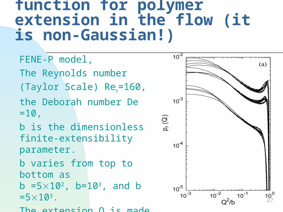
Radial distribution function for polymer extension in the flow (it is non-Gaussian!)

FENE-P model,

The Reynolds number

(Taylor Scale) Re=160,

the Deborah number De =10,

b is the dimensionless finite-extensibility parameter.

b varies from top to bottom as b =5102, b=103, and b =5103.

The extension Q is made dimensionless with the equilibrium end-to-end distance Q0.

P.Ilg, I. Karlin et al., 2002

28

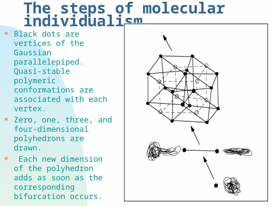
The steps of molecular individualism Black dots are vertices

of the Gaussian parallelepiped. Quasi-stable polymeric conformations are associated with each vertex.

Zero, one, three, and four-dimensional polyhedrons are drawn.

Each new dimension of the polyhedron adds as soon as the corresponding bifurcation occurs.

29

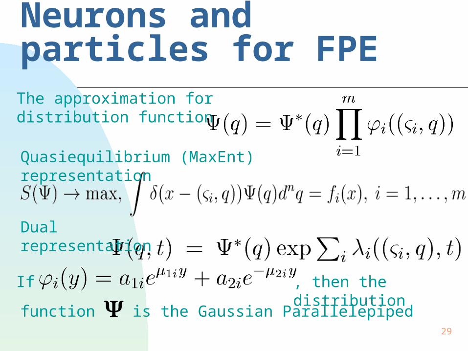
Neurons and particles for FPEThe approximation for distribution function

Quasiequilibrium (MaxEnt) representation

Dual representation

If , then the distribution

function is the Gaussian Parallelepiped

30

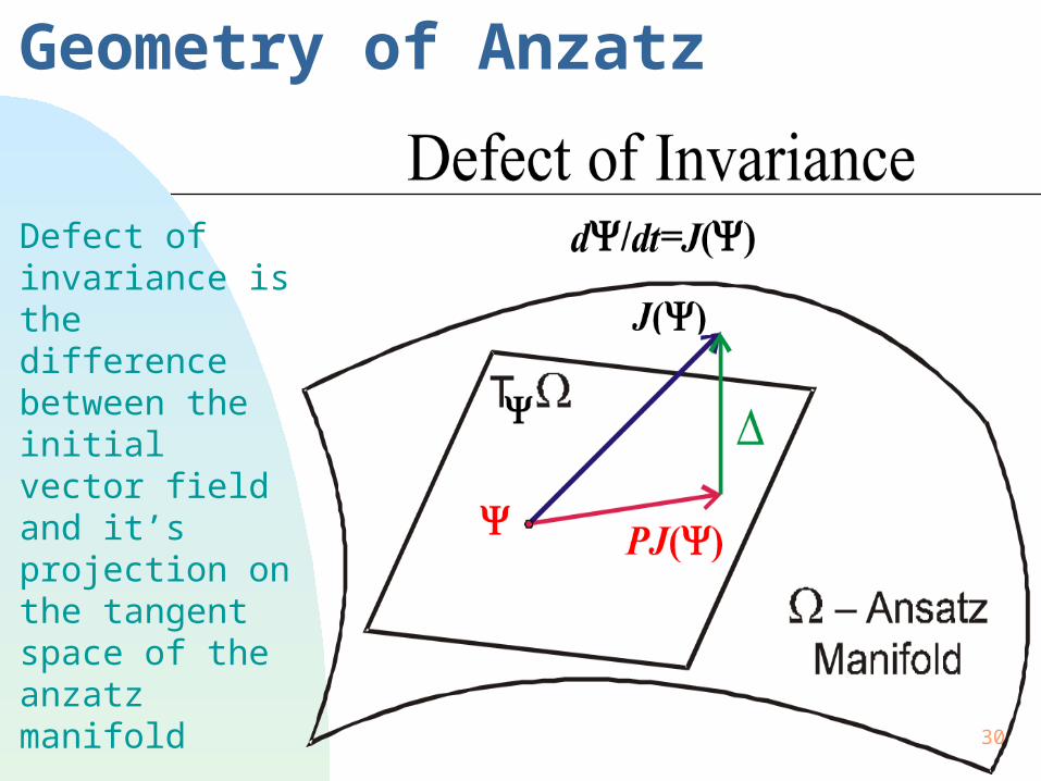
Geometry of Anzatz

Defect of invariance is the difference between the initial vector field and it’s projection on the tangent space of the anzatz manifold

31

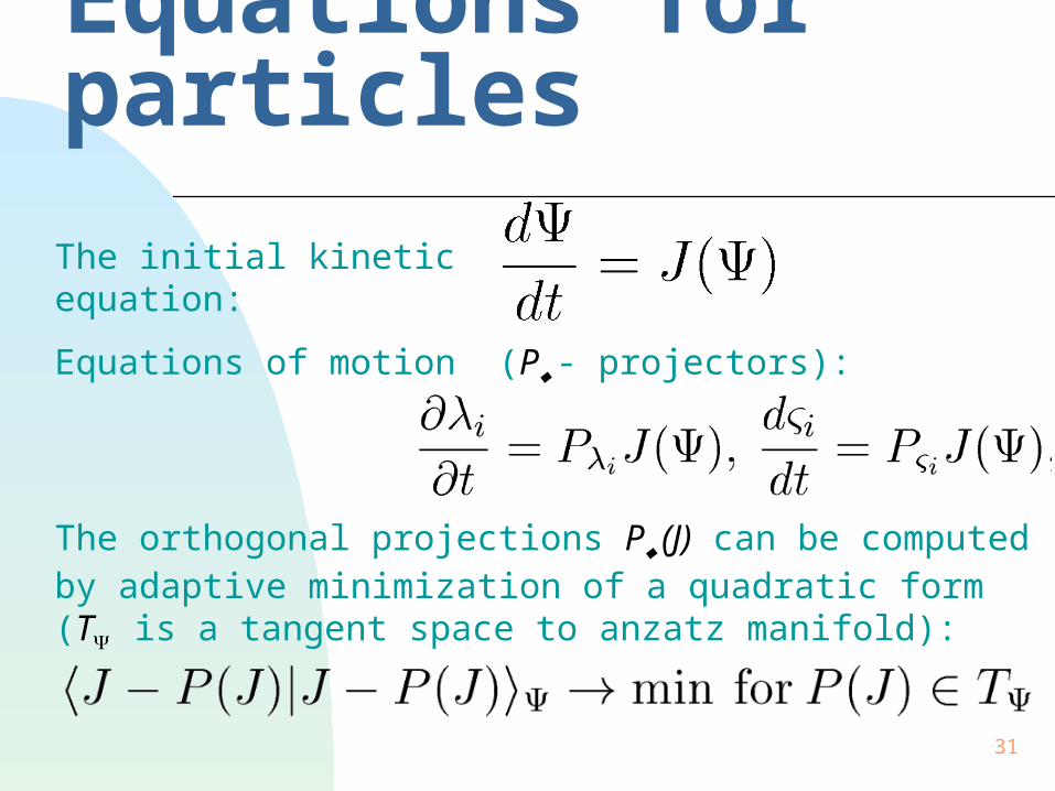
Equations for particles

Equations of motion (P - projectors):

The initial kinetic equation:

The orthogonal projections P (J) can be computed by adaptive minimization of a quadratic form (T is a tangent space to anzatz manifold):

32

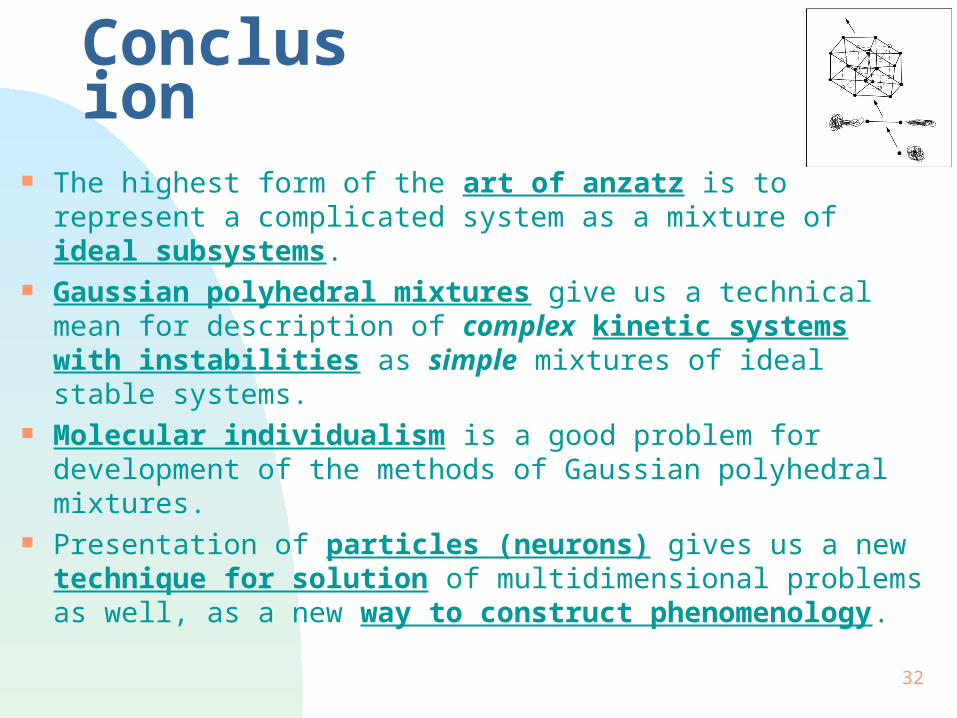
Conclusion

The highest form of the art of anzatz is to represent a complicated system as a mixture of ideal subsystems.

Gaussian polyhedral mixtures give us a technical mean for description of complex kinetic systems with instabilities as simple mixtures of ideal stable systems.

Molecular individualism is a good problem for development of the methods of Gaussian polyhedral mixtures.

Presentation of particles (neurons) gives us a new technique for solution of multidimensional problems as well, as a new way to construct phenomenology.

33

We work between complexity and simplicity and try to find one in the other

"I think the next century will be the century of complexity".

Stephen Hawking

But ... “Nature has a Simplicity, and therefore a great Beauty”.

Richard Feynman

34

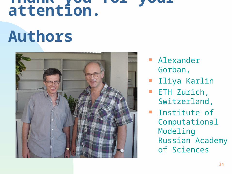
Thank you for your attention.Authors

Alexander Gorban, Iliya Karlin ETH Zurich,

Switzerland, Institute of

Computational Modeling Russian Academy of Sciences

35

36

Painted by Anna GORBAN