~ 1 ~ 

 

UNIVERSIDAD DE CÓRDOBA

Programa de Doctorado

DINÁMICA DE FLUJOS BIOGEOQUÍMICOS Y SU APLICACIÓN

TESIS DOCTORAL

DESCRIPCIÓN MULTIFRACTAL DE REDES ANTRÓPICAS Y NATURALES

 

MULTIFRACTAL DECRIPTION OF ANTHROPOGENIC AND NATURAL NETWORKS

 

Autora

Ana Belén Ariza Villaverde

Directores:

Prof. Dr. Francisco J. Jiménez Hornero

Prof. Dr. Eduardo Gutiérrez de Ravé Agüera

TITULO: DESCRIPCIÓN MULTIFRACTAL DE REDES ANTRÓPICAS YNATURALES - MULTRIFRACTAL DECRIPTION OFANTHROPOGENIC AND NATURAL NETWORKS

AUTOR: ANA BELÉN ARIZA VILLAVERDE

© Edita: Servicio de Publicaciones de la Universidad de Córdoba. Campus de RabanalesCtra. Nacional IV, Km. 396 A14071 Córdoba

www.uco.es/publicacionespublicaciones@uco.es

 

~ 2 ~ 

 

 

        

 

~ 3 ~ 

 

UNIVERSIDAD DE CÓRDOBA 

Programa de Doctorado

Dinámica de Flujos Biogeoquímicos y su Aplicación

TESIS DOCTORAL

Multifractal Decription of Anthropogenic and Natural Networks

Descripción Multifractal de Redes Antrópicas y Naturales

Tesis doctoral presentada por Ana Belén Ariza Villaverde, en satisfacción de los requisitos necesarios para optar al grado de Doctor por la Universidad de Córdoba con mención Doctorado Internacional, dirigida por los Drs. D. Francisco José Jiménez Hornero y D. Eduardo Gutiérrez de Ravé Agüera de la Universidad de Córdoba.

Los Directores:        El Doctorando: 

 

F.J. Jiménez Hornero      E. Gutiérrez de Ravé Agüera  A.B. Ariza Villaverde 

 

Córdoba, Febrero 2013 

 

~ 4 ~ 

 

                                

  

      

  TÍTULO  DE  LA  TESIS:  MULTIFRACTAL  DECRIPTION  OF  ANTHROPOGENIC  AND NATURAL NETWORKS   DOCTORANDO/A: ANA BELÉN ARIZA VILLAVERDE   

INFORME RAZONADO DEL/DE LOS DIRECTOR/ES DE LA TESIS (se hará mención a la evolución y desarrollo de la tesis, así como a trabajos y 

publicaciones derivados de la misma).  La  doctoranda  ha  desarrollado  su  actividad  en  el  programa  de  formación  de personal  docente  e  investigador  predoctoral  en  las  Universidades  Públicas  de Andalucía,  en  áreas  de  conocimiento  consideradas  deficitarias  por  necesidades institucionales  docentes  y  de  investigación.  En  este  marco,  ha  planificado, ejecutado  y  concluido  adecuadamente  el  trabajo  correspondiente  a  la  tesis doctoral que es objeto del presente documento.   Ana Belén Ariza Villaverde ha concluido brillantemente su formación predoctoral y, tal y como demuestra este trabajo, ha profundizado en el conocimiento y uso del análisis multifractal. Así, ha explorado con acierto  la aplicación esta  línea de investigación en la descripción de redes de origen natural y antrópico estudiando tres  casos  relevantes en escalas de  trabajo diferentes. Así, desde  la escala más pequeña  hasta  la más  grande,  ha  analizado  el  flujo  en  el  conjunto  de  canales presentes  en  un medio  poroso  idealizado,  la morfología  urbana  y  las  redes  de drenaje naturales. En el primer caso, determinó la conveniencia de usar el método de  análisis multifractal  conocido  como  Sandbox  para  describir  redes  frente  al algoritmo Box‐Counting, frecuentemente aplicado en trabajos previos. El estudio de  la morfología urbana  reveló que,  según  sea  su patrón  regular o  irregular, es necesario considerar una o varias dimensiones fractales para su descripción. Por último,  la  utilidad  del  análisis  multifractal  como  herramienta  de  ajuste  de 

parámetros  de  modelos  y  validación  de  sus  resultados  simulados  quedó demostrada  en  el  estudio  llevado  a  cabo  sobre  las  redes  de  drenaje  de  una cuenca.  Durante el periodo de  realización de  la  tesis doctoral destaca  la estancia que  la doctorando en el Dpto. de Ingeniería de la Universidad de Liverpool (Reino Unido) en  el  que  ha  profundizado  en  el  conocimiento  de  los  sistemas  de  información geográfica  aplicados  a  la  obtención  de  la  geometría  urbana  y  la  extracción  de redes de drenaje a partir de un modelo digital de elevaciones. Sin duda, de ambas cuestiones se ha beneficiado esta tesis doctoral ya que ha posibilitado parte de los estudios llevado a cabo en ella.  Los  resultados  obtenidos  en  esta  tesis  doctoral,  como  otros  derivados indirectamente  de  la  misma,  han  tenido  una  aceptable  difusión  a  nivel internacional  demostrada  por  la  siguiente  relación  de  publicaciones  y contribuciones  presentadas  en  congresos.  Este  hecho  resalta  el  carácter innovador de  la propuesta presentada a  la par que asegura su continuidad como línea de trabajo en el futuro.  Publicaciones en revistas incluidas en Journal Citation Reports (JCR)  Ariza‐Villaverde,  A.B.;  Jiménez‐Hornero,  F.J.;  Gutiérrez  de  Ravé,  E.  (en  prensa). Multifractal  Analysis  of  Axial Maps  Applied  to  the  Study  of Urban Morphology Computers, Environment and Urban Systems.   Ariza‐Villaverde,  A.B.;  Gutiérrez  de  Ravé,  E.;  Jiménez  Hornero,  F.J.;  Pavón‐Domínguez,  P.;  Muñoz‐Bermejo,  F.  (en  prensa).  Introducing  a  geographic information system as computer tool to apply the problem‐based learning process in  public  buildings  indoor  routing.  Computer  Applications  in  Engineering Education.  Jiménez Hornero, F.J.; Pavón‐Domínguez, P.; Gutiérrez de Ravé Agüera, E.; Ariza‐Villaverde, A.B.  2011.  Joint multifractal description  of  the  relationship between wind patterns and  land surface air temperature. Atmospheric Research, 99: 366‐376.  Jiménez Hornero, F.J.; Gutiérrez de Ravé, E.; Ariza‐Villaverde, A.B.; Giráldez,  J.V. 2010. Description of  the seasonal pattern  in ozone concentration  time series by using the strange attractor multifractal formalism. Environmental Monitoring and Assessment, 160: 229‐236. 

  Contribuciones en congresos internacionales  Ariza‐Villaverde, A.B.;  Pavón‐Domínguez,  P.;  Jiménez‐Hornero,  F.J.; Gutiérrez  de Ravé,  E.  2012.  Influence  of  the  urban  morphology  on  the  noise  pollution: Multifractal  analysis.  Urban  Environmental  Pollution.  Amsterdam  (Los  Países Bajos).  Ariza‐Villaverde, A.B.;  Pavón‐Domínguez,  P.;  Jiménez‐Hornero,  F.J.; Gutiérrez  de Ravé,  E.  2012. Description  of  urban  environment  applying multifractal  analysis. Urban Environmental Pollution. Amsterdam (Los Países Bajos).  Pavón‐Domínguez,  P.; Ariza‐Villaverde, A.B.;  Jiménez‐Hornero,  F.J.; Gutiérrez  de Ravé Agüera, E. 2012. Temperature  influence on  the ozone  scaling behaviour  in the  metropolitan  area  of  Seville.  Urban  Enviromental  Pollution.  Amsterdam (Países Bajos).  Pavón‐Domínguez,  P.; Ariza‐Villaverde, A.B.;  Jiménez‐Hornero,  F.J.; Gutiérrez  de Ravé Agüera, E. 2012. Characterizing the temporal relationships between ground‐level  ozone  and  several meteorological  variables  by  using  the  joint multifractal approach. Urban Enviromental Pollution. Amsterdam (Países Bajos).  Ariza‐Villaverde, A.B.;  Pavón‐Domínguez,  P.;  Jiménez‐Hornero,  F.J.; Gutiérrez  de Ravé Agüera, E. 2010. Application of the  joint multifractal analysis for describing the  influence of nitrogen dioxide on ground‐level ozone concentrations. General Assembly.  European  Geosciences  Union.  Viena  (Austria).  Geophysical  Research Abstracts. Vol. 12, EGU2010‐474.  Pavón‐Domínguez,  P.; Ariza‐Villaverde, A.B.;  Jiménez‐Hornero,  F.J.; Gutiérrez  de Ravé  Agüera,  E.  2010.  Analysis  of  some meteorological  time  series  relevant  in urban  environments  by  applying  the  multifractal  analysis.  General  Assembly. European  Geosciences  Union.  Viena  (Austria).  Geophysical  Research  Abstracts. Vol. 12, EGU2010‐1261.  A.B. Ariza‐Villaverde, F.J.  Jiménez‐Hornero,  J.V. Giráldez, P. Pavón‐Domínguez, E. Gutiérrez  de  Ravé  Agüera,  T.  Vanwalleghem.  Multifractal  description  of  the idealised  porous  media  geometry  influence  on  the  simulated  flow  velocity. Optimizing and Integrating Prediction of Agricultural Soil and Water Conservation Models at Different Scales (2010). Baeza (Jaén, España). 

  Por todo ello, se autoriza la presentación de la tesis doctoral.  

Córdoba, 21 de Noviembre de 2012  

Firma del/de los director/es    

   Fdo.: Francisco José Jiménez Hornero       Fdo.: Eduardo Gutiérrez de Ravé Agüera 

 

~ 5 ~ 

 

     

To my parents

 

~ 6 ~ 

 

 

~ 7 ~ 

 

Agradecimientos

Siempre he pensado que una persona es como un trozo de barro en manos de un alfarero o como el plano de una casa en manos de un maestro de obra..., al principio es un sueño, pero en manos de un gran equipo puede llegar a ser una realidad.

En este sueño puedo considerar a los dos mejores arquitectos, mis directores de tesis Francisco y Eduardo. Agradecerles su confianza en mí por haberme concedido el honor de realizar con ellos mi tesis doctoral. Por toda su gran entrega, ayuda y apoyo que han demostrado a lo largo de estos años. Gracias a ellos, ha sido posible llegar hasta aquí.

Como no mencionar a mis padres, María y Rafael, pilares fundamentales en mi vida, que han hecho posible que este sueño se haga realidad. Sin ellos, no lo hubiera conseguido. Luchadores natos y un gran ejemplo a seguir. Sin su apoyo no habría llegado tan lejos. Ellos, junto con mis hermanos Eva y Rafa que junto a Noel e Isabel, mis cuñados, siempre me han animado y ayudado, estando siempre a mi lado cuando los he necesitado.

Este proyecto no hubiera sido posible sin el apoyo de mi marido, Francisco Manuel, una de las personas más importantes de mi vida. Por estar siempre a mi lado, por su gran optimismo y forma de ver la vida, que hace que cada mañana me levante con una gran sonrisa.

A mi abuela, por estar a mi lado y preocuparse diariamente por mí, siempre preguntándome que cuando voy a dejar de estudiar, quisiera agradecerle su compresión y cariño por todos aquellos momentos en los que he estado muy ocupada y no he podido dedicarle el tiempo que se merece.

Agradecerles a mis suegros, Loli y Diego, su ayuda y dedicación. No podría olvidar a mis tíos, Lola, José, Manolo y Juan Antonio y a mi prima

 

~ 8 ~ 

 

Miriam, que siempre se han interesado y alegrado por mí. A mi tío cura, José Manuel, por todo su cariño y sus buenos consejos.

A mi buen amigo Miguel Ángel, por toda la ayuda prestada y estar siempre a mi lado cuando lo he necesitado. Agradecerle la elaboración de la portada de esta tesis, en la cual ha puesto un gran entusiasmo e ilusión. Y como agradecerle el regalo más agradable de mi vida, “Wawi” mi mascota, esa personita que me da ese puntito de felicidad todos los días.

Hacer una mención muy especial a mis grandes amigos de Liverpool, Hassan y Dean, por hacer que mi estancia predoctoral en el Reino Unido fuese mucho más enriquecedora, portándose como una verdadera familia.

Por último, me gustaría agradecer a mis compañeros de trabajo Fernando, Antonio, Nazareth, Pablo y Jesús por su ayuda a lo largo de estos años y por hacer que el trabajo fuese más ameno.

Muchas gracias a todos por lo que hemos logrado  

 

 

 

~ 9 ~ 

 

 

“Sometimes we feel that what we do is just a drop in the bucket, but the ocean would be less

if it needed that missing drop”

Mother Teresa of Calcutta (1910-1997)

 

~ 10 ~ 

 

 

~ 11 ~ 

 

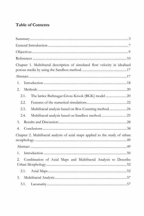
Table of Contents

Summary ..................................................................................................................... 3

General Introduction ................................................................................................ 7

Objectives ................................................................................................................... 9

References ................................................................................................................ 10

Chapter 1. Multifractal description of simulated flow velocity in idealised porous media by using the Sandbox method. ..................................................... 17

Abstract ..................................................................................................................... 17

1. Introduction ................................................................................................... 18

2. Methods .......................................................................................................... 20

2.1. The lattice Bathnagar-Gross-Krook (BGK) model ......................... 20

2.2. Features of the numerical simulations................................................ 22

2.3. Multifractal analysis based on Box-Counting method. .................... 24

2.4. Multifractal analysis based on Sandbox method. .............................. 25

3. Results and Discussion ................................................................................. 28

4. Conclusions .................................................................................................... 38 

Chapter 2. Multifractal analysis of axial maps applied to the study of urban morphology. ............................................................................................................. 49

Abstract ................................................................................................................... 49

1. Introduction ................................................................................................... 50

2. Combination of Axial Maps and Multifractal Analysis to Describe Urban Morphology ................................................................................................ 52

2.1. Axial Maps .............................................................................................. 52

3. Multifractal Analysis ...................................................................................... 57

3.1. Lacunarity ............................................................................................... 57

 

~ 12 ~ 

 

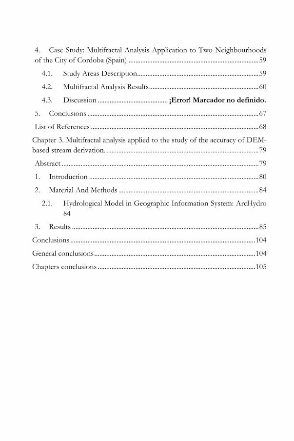
4. Case Study: Multifractal Analysis Application to Two Neighbourhoods of the City of Cordoba (Spain) ............................................................................ 59

4.1. Study Areas Description ....................................................................... 59

4.2. Multifractal Analysis Results ................................................................ 60

4.3. Discussion ......................................... ¡Error! Marcador no definido.

5. Conclusions .................................................................................................... 67

List of References .................................................................................................. 68 

Chapter 3. Multifractal analysis applied to the study of the accuracy of DEM-based stream derivation. ......................................................................................... 79

Abstract ................................................................................................................... 79

1. Introduction ................................................................................................... 80

2. Material And Methods .................................................................................. 84

2.1. Hydrological Model in Geographic Information System: ArcHydro 84

3. Results ............................................................................................................. 85

Conclusions ............................................................................................................ 104

General conclusions .............................................................................................. 104

Chapters conclusions ............................................................................................ 105

 

~ 13 ~ 

 

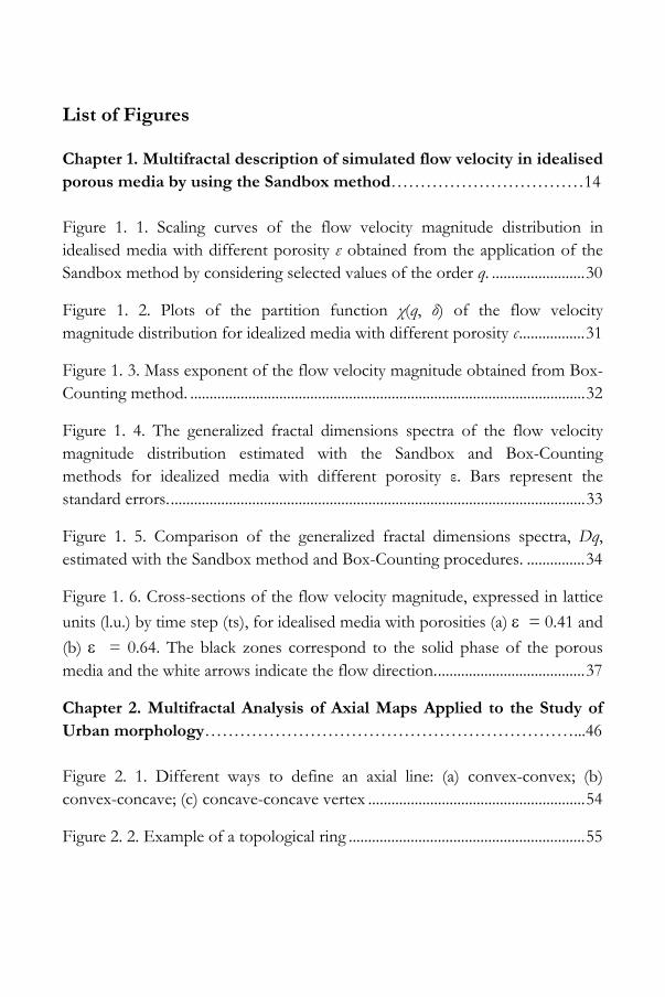
List of Figures Chapter 1. Multifractal description of simulated flow velocity in idealised porous media by using the Sandbox method……………………………14 Figure 1. 1. Scaling curves of the flow velocity magnitude distribution in idealised media with different porosity ε obtained from the application of the Sandbox method by considering selected values of the order q. ........................ 30

Figure 1. 2. Plots of the partition function χ(q, δ) of the flow velocity magnitude distribution for idealized media with different porosity є ................. 31

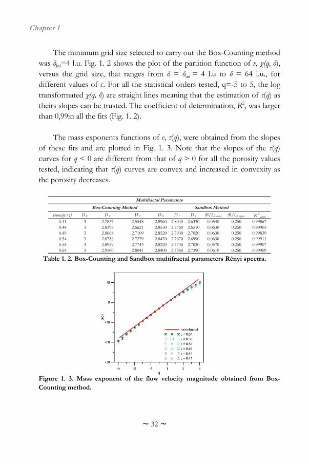
Figure 1. 3. Mass exponent of the flow velocity magnitude obtained from Box-Counting method. ...................................................................................................... 32

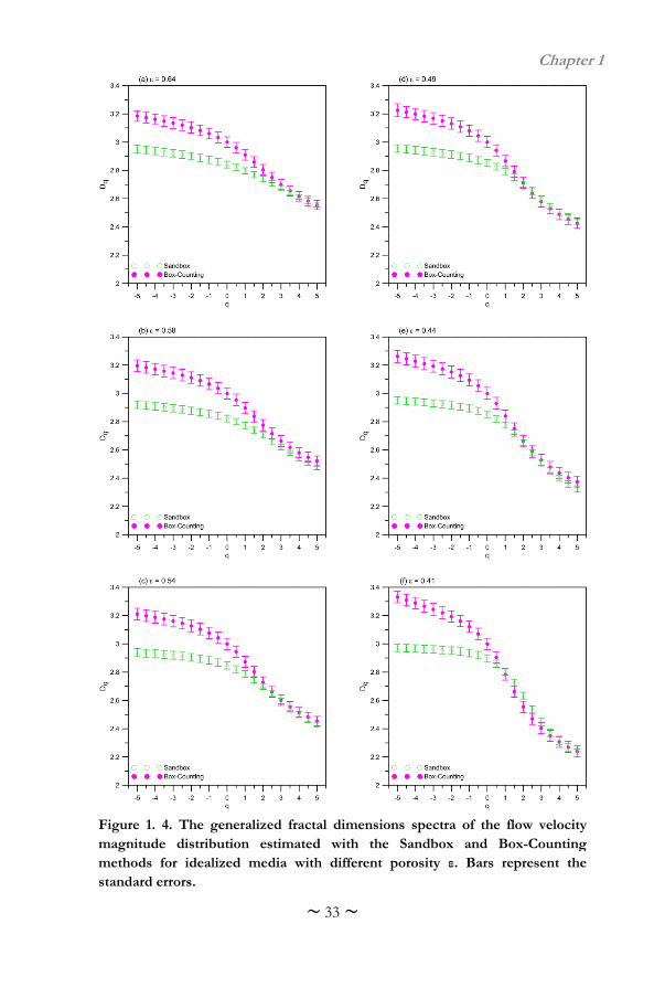
Figure 1. 4. The generalized fractal dimensions spectra of the flow velocity magnitude distribution estimated with the Sandbox and Box-Counting methods for idealized media with different porosity ε. Bars represent the standard errors. ........................................................................................................... 33

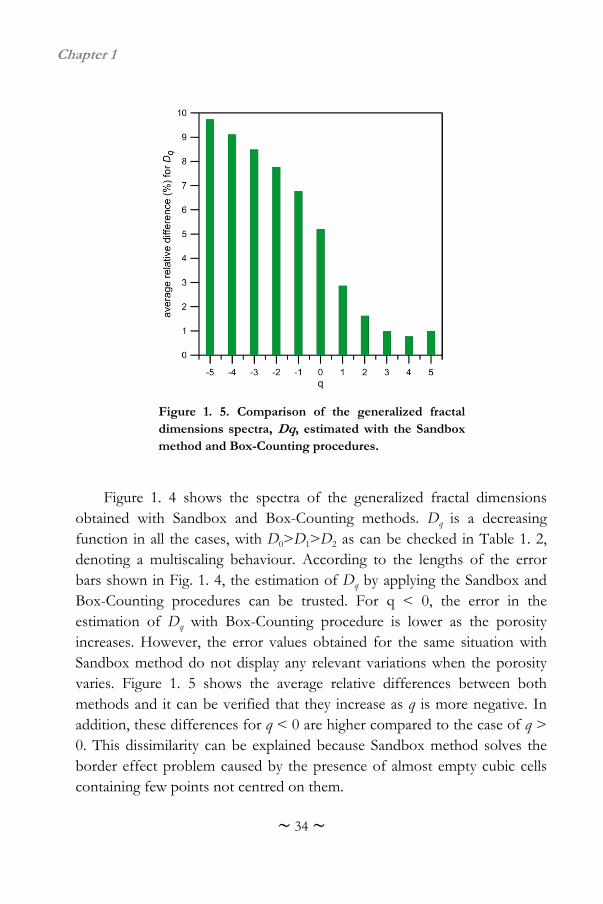
Figure 1. 5. Comparison of the generalized fractal dimensions spectra, Dq, estimated with the Sandbox method and Box-Counting procedures. ............... 34

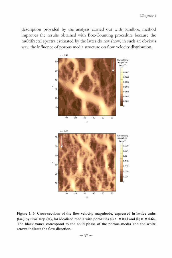
Figure 1. 6. Cross-sections of the flow velocity magnitude, expressed in lattice

units (l.u.) by time step (ts), for idealised media with porosities (a) = 0.41 and

(b) = 0.64. The black zones correspond to the solid phase of the porous media and the white arrows indicate the flow direction. ...................................... 37

Chapter 2. Multifractal Analysis of Axial Maps Applied to the Study of Urban morphology………………………………………………………...46 Figure 2. 1. Different ways to define an axial line: (a) convex-convex; (b) convex-concave; (c) concave-concave vertex ........................................................ 54

Figure 2. 2. Example of a topological ring ............................................................. 55

 

~ 14 ~ 

 

Figure 2. 3. Location of the city of Cordoba ......................................................... 56

Figure 2. 4. Areas selected for this work ................................................................ 56

Figure 2. 5. The generalized dimension spectra. Vertical bars represent the standard error of the computed multifractal average parameters ....................... 63

Chapter 3. Multifractal analysis of synthetic rivers network accuracy.....76

Figure 3. 1. Location of study area .......................................................................... 83

Figure 3. 2. Scheme of D8 method ......................................................................... 84

Figure 3. 3. Scales curves .......................................................................................... 87

Figure 3. 4. Rényi spectra .......................................................................................... 90

Figure 3. 5. River map generated with ArcHydro tool and photogrammetric restitution ................................................................................................................... 91

 

~ 15 ~ 

 

List of Tables Chapter 1. Multifractal description of simulated flow velocity in idealised porous media by using the Sandbox method……………………………14 Table 1. 1. Statistical parameters of the flow velocity magnitude, v, simulated for idealized porous media with different porosity, ε ........................................... 29

Table 1. 2. Box-Counting and Sandbox multifractal parameters Rényi spectra 32

Chapter 2. Multifractal Analysis of Axial Maps Applied to the Study of Urban Morphology……………………………………………………....46 Table 2. 1. Features and statistical analysis of the different axial maps ............. 60

Table 2. 2. Blocks statistical analysis ....................................................................... 60

Table 2. 3. Multifractal parameters obtained from applying the Sandbox method ......................................................................................................................... 61

Chapter 3. Multifractal analysis of synthetic rivers network accuracy.....76

Table 3. 1. Multifractal parameters for each study area. ....................................... 89

Table 3. 2. Flow accumulation threshold value selected. ..................................... 86

 

 

 

 

 

~ 16 ~ 

 

  

 

 

Resumen

~ 1 ~ 

 

Resumen

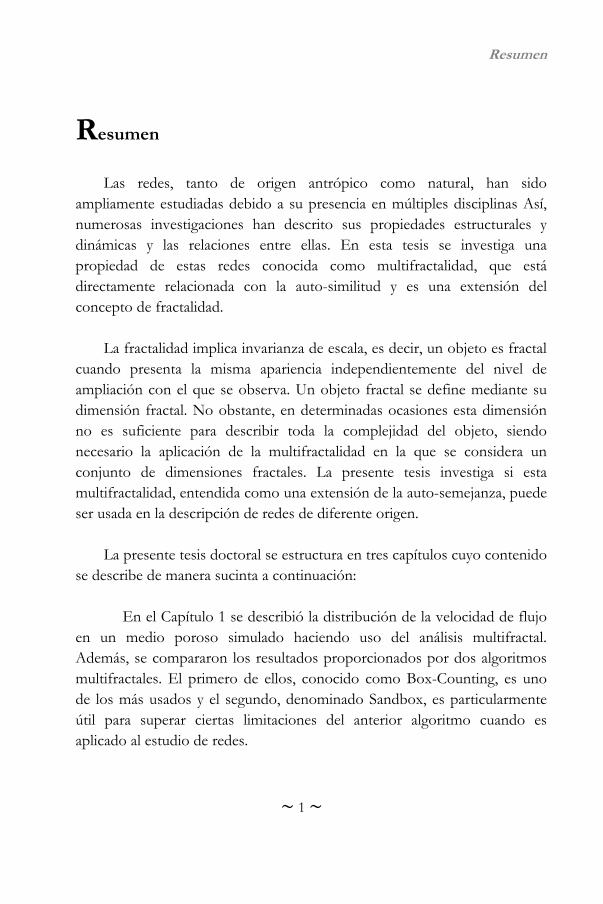
Las redes, tanto de origen antrópico como natural, han sido ampliamente estudiadas debido a su presencia en múltiples disciplinas Así, numerosas investigaciones han descrito sus propiedades estructurales y dinámicas y las relaciones entre ellas. En esta tesis se investiga una propiedad de estas redes conocida como multifractalidad, que está directamente relacionada con la auto-similitud y es una extensión del concepto de fractalidad.

La fractalidad implica invarianza de escala, es decir, un objeto es fractal

cuando presenta la misma apariencia independientemente del nivel de ampliación con el que se observa. Un objeto fractal se define mediante su dimensión fractal. No obstante, en determinadas ocasiones esta dimensión no es suficiente para describir toda la complejidad del objeto, siendo necesario la aplicación de la multifractalidad en la que se considera un conjunto de dimensiones fractales. La presente tesis investiga si esta multifractalidad, entendida como una extensión de la auto-semejanza, puede ser usada en la descripción de redes de diferente origen.

La presente tesis doctoral se estructura en tres capítulos cuyo contenido

se describe de manera sucinta a continuación:

En el Capítulo 1 se describió la distribución de la velocidad de flujo en un medio poroso simulado haciendo uso del análisis multifractal. Además, se compararon los resultados proporcionados por dos algoritmos multifractales. El primero de ellos, conocido como Box-Counting, es uno de los más usados y el segundo, denominado Sandbox, es particularmente útil para superar ciertas limitaciones del anterior algoritmo cuando es aplicado al estudio de redes.

Resumen 

~ 2 ~ 

 

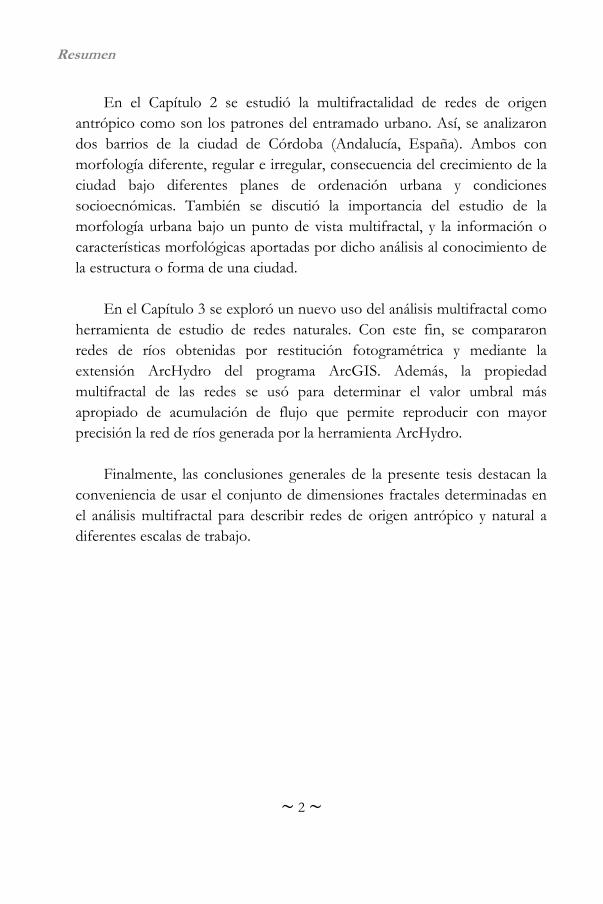
En el Capítulo 2 se estudió la multifractalidad de redes de origen antrópico como son los patrones del entramado urbano. Así, se analizaron dos barrios de la ciudad de Córdoba (Andalucía, España). Ambos con morfología diferente, regular e irregular, consecuencia del crecimiento de la ciudad bajo diferentes planes de ordenación urbana y condiciones socioecnómicas. También se discutió la importancia del estudio de la morfología urbana bajo un punto de vista multifractal, y la información o características morfológicas aportadas por dicho análisis al conocimiento de la estructura o forma de una ciudad.

En el Capítulo 3 se exploró un nuevo uso del análisis multifractal como

herramienta de estudio de redes naturales. Con este fin, se compararon redes de ríos obtenidas por restitución fotogramétrica y mediante la extensión ArcHydro del programa ArcGIS. Además, la propiedad multifractal de las redes se usó para determinar el valor umbral más apropiado de acumulación de flujo que permite reproducir con mayor precisión la red de ríos generada por la herramienta ArcHydro.

Finalmente, las conclusiones generales de la presente tesis destacan la

conveniencia de usar el conjunto de dimensiones fractales determinadas en el análisis multifractal para describir redes de origen antrópico y natural a diferentes escalas de trabajo.

Summary

~ 3 ~ 

 

Summary

 

Networks, both anthropogenic and natural, have been widely studied due to its presence in multiple disciplines. Thus, numerous studies have described their structural and dynamic properties and the relationships between them. In this thesis it is investigated a property of these networks known as multifractality, which is directly related to self-similarity and is an extension of the concept of fractality.

Fractality implies scale invariance (i.e., an object is fractal when it

presents the same appearance regardless of the magnification level with which it is observed). A fractal object is defined by its fractal dimension. However, on occasion this dimension is not enough to describe the complexity of the object, requiring the application of multifractality in what is considered a set of fractal dimensions. This thesis investigates whether this multifractality, understood as an extension of self-similarity, can be used in the description of networks with different origin.

This thesis is divided into three chapters which contents are described

succinctly below:

In Chapter 1 there was elucidated the distribution of flow velocity in a simulated porous medium using multifractal analysis. Furthermore, we compared the results provided by two multifractal algorithms; the first, known as Box-Counting, is one of the most used, and the second, called Sandbox, is particularly useful to overcome certain limitations of the preceding when applied studying networks.

In Chapter 2 we studied multifractality of anthropogenic networks such

as urban fabric patterns. Thus, we analyzed two neighborhoods in the city

Summary 

~ 4 ~ 

 

of Córdoba (Andalusia, Spain) both with different morphologies, regular and irregular, due to the growth of the city under different urban planning and socioeconomic conditions. It was also discussed the importance of the study of urban morphology under a multifractal standpoint, and morphological information provided by such analysis to the knowledge of the structure or shape of a city.

In Chapter 3, we explored a new use of multifractal analysis as a tool

for the study of natural networks. To this end, we compared networks of rivers obtained by photogrammetric restitution and by the extension ArcHydro from ArcGIS software. Furthermore, the multifractal property of the networks was used to determine the most appropriate threshold value of flow accumulation that allows reproducing more accurately the network of rivers generated by the computer tool ArcHydro.

Finally, the general conclusions of this thesis highlight the convenience

of using the set of fractal dimensions determined by multifractal analysis to describe networks of anthropogenic and natural networks at different scales of implementation.

 

~ 5 ~ 

 

General Introduction & Objectives

 

“Fractal geometry will make you see

everything differently. There is danger in reading further.

You risk the loss of your childhood visions of Clouds, forest, galaxies, leaves, feathers, rocks,

Mountains, torrents of water, carpets, bricks and much else besides.

Never again will your interpretation of these things be quite the same.”

Michael F. Barnsley (1988)

 

~ 6 ~ 

 

 

 

~ 7 ~ 

 

General Introduction

The study of networks has attracted an enormous amount of interest in the last few years (Boccaletti et al., 2006). A large amount of systems can be regarded as networks: social relationships between individuals (Toivonen et al., 2006; Wong et al., 2006), molecular interactions and transformations (Barabási & Oltvai, 2004), transportation or communication systems (Latora & Marchiori, 2002; Wang et al., 2011), internet (Pastor-Satorras, et al., 2001; Wu et al., 2011), power grids (Crucitti et al., 2004; Sun, 2005), and even urban streets are composed by networks(Porta et al., 2006; Jiang, 2007).

A network is defined as a set of items, called nodes, with connections between them better known as edges (Newman, 2003). One of the properties of networks is self-similarity which is commonly related to fractality. Self-similarity essentially means that there is some correspondence between parts of the object and the total characteristics of it (i.e., they look similar under different magnifications level or range of scales, being able to build a simplified theory that captures the main features of these objects). When fractals appear identical at different scales the self-similarity is exact (e.g., the Sierpinski triangle and the Koch snowflake exhibit exact self-similarity). In the case of fractals, those that appear approximately (but not exactly) identical at different scales are quasi-self-similar (e.g., the Mandelbrot set). On the other hand, when each part of an object has statistical measures which are conserved across different scales, the self-similarity is defined as statistical; a prominent example is the coast of Britain introduced by Mandelbrot in 1967.

 

Fractal objects are defined, through the fractal dimension, as a measure of complexity (Feder, 1988). The fractal dimension is a non-integer number that quantifies the density of the fractal in the metric space, and it is commonly used as a tool to identify how complex a fractal is, allowing its comparison with another fractal (Mandelbrot, 1982; Tricot, 1995; Schroeder

 

~ 8 ~ 

 

et al., 2009). However, sometimes just a single fractal dimension might not always be enough to characterize complex and heterogeneous behaviour. In order to solve this deficiency the multifractal approach is developed to describe the data with a set of fractal dimensions instead of a single value. This approach is originally introduced by Mandelbrot, 1972 and 1974, in the discussion of turbulence and, later, expanded to many other contexts (Mandelbrot, 1982). Multifractal formalisms involve that self-similar measures can be represented as a combination of intertwined fractal sets each of which characterized by its singularity strength and fractal dimension. This set is called multifractal spectrum and the method of variability characterization, based on the multifractal spectrum, is referred to as a multifractal analysis (Frish and Parisi, 1985).

Multifractals are more flexible in describing locally irregular phenomena than monofractals, which are governed by single fractal dimension. Moreover, other advantage using this approach is that the multifractal parameters can be independent of the size of the studied object (Cox & Wang, 1993). On the other hand, multifractal analysis transforms irregular data into a more compact form and amplifies slight differences among the variables’ distribution (Lee, 2002).

 

Multifractals approach has been used along the last two decades in many studies fields. They are been applied to characterize natural phenomena such as the spatial variability of soil properties (Kravchenko et al., 1999; Zeleke & Cheng, 2004) and rainfall distributions (Olson & Niemczynowicz, 1996; Kim et al, 2008), the spatial and temporal distribution of environmental pollution (Salvadori et al, 1997; Shi et al, 2009), and even earthquakes (Hirabayashi et al, 1992; Zamani et al, 2009). Other discipline where multifractal analysis has been utilized is medicine: studying the cellular and neurons morphology (Smith et al, 1996; Fernández et al, 1999), characterizing volumetric texture in medical imagines (Lopes et al, 2011), detecting microcalcifications in digital mammograms (Stojic, 2006) as well as classifying malign tissues from normal and benign (Andjelkovic, 2008),

 

~ 9 ~ 

 

among others. Equally, this approach has been employed in economy to analyse crude oil prices (Alvarez-Ramirez, 2002), price fluctuations of stock and commodities (Matia et al, 2003), market volatility (Chen and Wu, 2011) and stock market inefficiency (Zunino et al, 2008), etc.

This thesis investigates the suitability of applying multifractal approach to the description of different types of networks, anthropogenic and naturals, and how this method is able to extract different features of the network in 2D and 3D.

Objectives

In summary, there is a promising approach, based on the multifractality

property of some objects, which help to describe them in a more suitable way further than other traditional methods that are not able to perceive slight differences among the variables distribution. Therefore, the main objectives of this thesis are:

i. To characterize different kinds of networks: flow in idealised

porous media, urban patterns, and river morphologies.

ii. Comparison of multifractal algorithms: Box-Counting and Sandbox.

iii. To extend the use of multifractal as a pattern recognition tool.

iv. To use multifractal analysis as a tool to check the validity of results provided by models.

 

~ 10 ~ 

 

References Alvarez-Ramirez, J., Cisneros, M., Ibarra-Valdez, C., & Soriano, A. (2002).

Multifractal Hurst analysis of crude oil prices. Phys Stat Mech Appl, 313 (3 – 4), 651 – 670.

Andjelkovic, J., Zivic, N., & Reljin, B. (2008). Application of Multifractal

Analysis on Medical Images. Wseas Transactions on Information Science & Applications, 5(11), 1561 – 1572.

Barabási, A.L. & Oltvai, Z.N. (2004). Network biology: understanding the cell's

functional organization. Nat. Rev. Genet., 5, 101 – 113. Boccalettia, S., Latora, V., Moreno, Y., Chavez, M. & Hwang, D.-U. (2006).

Complex networks: structure and dynamics. Phys. Rep., 424: 175 – 308. Chen, H. & Wu, C. (2011). Forecasting volatility in Shanghai and Shenzhen

markets based on multifractal analysis. Phys Stat Mech Appl, 390 (16), 2926 – 2935.

Cox, L.B., & Wang, J.S.Y. (1993). Fractals surfaces: Measurement and

applications in earth sciences. Fractals, 1, 87 – 115. Crucitti, P., Latora, V., & Marchiori, M. (2004). A topological analysis of the

Italian electric power grid. Physica A, 338, 92 – 97. Feder, J. (1988). Fractals. New York: Plenum Press. Fernández, E., Bolea, J.A., Ortega, G., & Louis, E. (1999). Are neurons

multifractals?. J Neorosci, 89, 151 – 157. Frisch, U. & Parisi, G. (1985). Frisch U, Parisi G. 1985. On the singularity

structure of fully developed turbulence. In Turbulence and

 

~ 11 ~ 

 

Predictability in Geophysical Fluid Dynamics and Climate Dynamics. Ghil M, Benzi R, Parisi G (eds). North-Holland: New York; 84 – 88.

Hirabayashi, T., Ito, K., & Yoshi, T. (1992). Multifractal analysis of

earthquakes. Pure Appl Geophys, 138(4), 591 – 610. Jiang, B. (2007). A topological pattern of urban street networks: Universality

and peculiarity. Physica A, 384, 647 – 655. Lopes, R., Dubois,P., Bhouri, I., Bedoui, M.H., Maouche, S., and Betrouni, N.

(2011). Local fractal & multifractal features for volumic texture characterization. Pattern Recogn, 44(8), 1690 – 1697.

Matia, K., Ashkenazy, Y., & Stanley, H.E. (2003). Multifractal properties of

price fluctuations of stock and commodities. Europhys Lett, 61(3), 422 – 428.

Kravchenko, A.N., Boast, C.W., & Bullock, D.G. (1999). Multifractal analysis

of soil spatial variability. Agron. J., 91, 1033 – 1041. Kim, S.Y., Lim, G.C., Chang, K.H., Jung, J.W., and Kim, K., & Park, C.H.

(2008). Multifractal analysis of rainfalls in Korean peninsula. J. Korean Phys. Soc., 52(3), 669 – 672.

Latora, V., & Marchiori, M. (2002). Is the Boston subway a small-world

network? Physica A, 314, 109 – 113. Lee, C.K. (2002). Multifractals characteristics in air pollutant concentration

times series. Water Air Soil Pollut., 135, 389 – 409. Newman, M.E.J (2003). The structure and function of complex networks.

SIAM Rev., 45 (2), 167 – 256. Mandelbrot, B. (1967). How Long Is the Coast of Britain? Statistical Self-

Similarity and Fractional Dimension. Science, 156, 636 – 638.

 

~ 12 ~ 

 

Mandelbrot, B. B. (1972). Possible refinement of the lognormal hypothesis concerning the distribution of energy dissipation in intermittent turbulence. In: Statistical Models and Turbulence. Lecture Notes in Physics, 12, 333 – 351.

Mandelbrot, B. B. (1974). Intermittent turbulence in self-similar cascades:

divergence of high moments and dimension of the carrier.  J. Fluid Mech., 62, 331 – 358.

Mandelbrot, B.B. (1982). The Fractal Geometry of Nature. New York: W.H.

Freeman. Olsson, J., & Niemczynowicz, J. (1996). Multifractal analysis of daily spatial

rainfall distributions. J. Hydrol., 118(1-2), 29 – 43. Pastor-Satorras, R., Vázquez, A., & Vespignani, A. (2001). Dynamical and

correlation properties of the internet. Phys. Rev. Lett., 87(25), 258701 - 1 – 258701 - 4.

Porta, S., Crucitti, P. & Latora, V. (2006). The network analysis of urban

streets: a dual approach. Physica A, 369, 853 – 866. Salvadori, G., Ratti, S.P., & Belli, G., (1997). Fractal and multifractal approach

to environmental pollution. Environ. Sci. Pollut. Res., 4(2), 91 – 98. Stojić, T., Reljin, I., & Reljin, B. (2006). Adaptation of multifractal analysis to

segmentation of microcalcifications in digital mammograms. Phys Stat Mech Appl, 367, 494 – 508.

Tricot, C. (1995). Curves and Fractal Dimension. Paris: Springer-Verlag. Schroeder, M. (2009). Fractals, Chaos, Power Laws: Minutes from an Infinite

Paradise. New York: W.H. Freeman.

 

~ 13 ~ 

 

Smith, T.G., Lange, G.D., & Marks, W.B. (1996). Fractal methods and results in cellular morphology - Dimensions, lacunarity and multifractals. J Neurosci, 69(2), 123 – 136.

Sun, K. (2005). Complex Networks Theory: A New Method of Research in

Power Grid. IEEE/PES Transmission and Distribution Conference and Exhibition: Asia and Pacific. Dalian, China.

Toivonen, R., Onnela, J.P., Saramäki, J., Hyvönen, J., & Kaski, K. (2006). A

model for social networks. Physica A, 371, 851 – 860. Wang, J., Mo, H., Wang, F. & Jin, F. (2011). Exploring the network structure

and nodal centrality of China’s air transport network: a complex network approach. J. Transp. Geogr., 19: 712 – 721.

Wong, L.H., Pattison, P. & Robins, G. (2006). A spatial model for social

networks. Physica A, 360, 99 – 120. Wu, X., Yu, K., & Wang X. (2011). On the growth of internet application

flows: a complex network perspective. IEEE INFOCOM 2011. Shanghai, China.

Zamani, A., & Agh-Atabai, M. (2009). Temporal characteristics of seismicity in

the Alborz and Zagros regions of Iran, using a multifractal approach. J Geodyn, 47(5), 271 – 279.

Zeleke, B.T., & Si, C.B. (2004). Scaling properties of topographic indices and

crop yield: multifractal and joint multifractal approaches. Agron. J., 96, 1082 – 1090.

Zunino,L., Tabakd, B.M., Figliola, A., Pérez, D.G., Garavaglia, M., & Rosso,

O.A. (2008). A multifractal approach for stock market inefficiency. Physica A, 387, 6558 – 6566.

 

~ 14 ~ 

 

 

~ 15 ~ 

 

Chapter 1

“A las plantas, a los animales y a los humanos nos recorre por dentro al menos un doble río. Para que la sangre llegue a todas partes, las

venas se hacen cuenca, cauce y caudal. Es más, para que el chisporroteo de las ideas, los

recuerdos y las emociones nos concedan la condición humana, necesitamos el enramado

río de las neuronas, que son puro plagio de la voluptuosidad que comparten las estructuras

fractales que el agua inicia.”

Joaquín Araújo (1947- )

 

~ 16 ~ 

 

Chapter 1

~ 17 ~ 

 

Chapter 1. Multifractal

description of simulated flow velocity in idealised porous

media by using the Sandbox method.

Abstract

The spatial description of flows in porous media is a main issue due to their influence on processes that take place inside. In addition to descriptive statistics, the multifractal analysis based on the Box-Counting fixed-size method has been used during last decade to study some porous media features. However, this method gives emphasis to domain regions containing few data points that spark the biased assessment of generalized fractal dimensions for negative moment orders. This circumstance is relevant when describing the flow velocity field in idealised three-dimensional porous media. The application of the Sandbox method is explored in this work as an alternative to the Box-Counting procedure for analyzing flow velocity magnitude simulated with the lattice model approach for six media with different porosities. According to the results, simulated flows have multiscaling behaviour. The multifractal spectra obtained with the Sandbox method reveal more uniformity in the distribution of flow velocity magnitudes as porosity increases. This situation is not so evident for the multifractal spectra estimated with the Box-Counting method. As a consequence, the description of the influence of porous media structure on flow velocity distribution provided by the Sandbox method improves the results obtained with the Box-Counting procedure.

KEYWORDS: Flow velocity; lattice Boltzmann model; multifractal analysis, porous media; Sandbox method.

Chapter 1

~ 18 ~ 

 

1. Introduction

Many relevant biogeochemical phenomena in porous media are greatly influenced by flows that take place in them (Rinck-Pfeiffer et al, 2000; Islam et al, 2001; Thullner et al, 2005). In order to improve the predictability of flow processes in porous media, factors that control the fluid distribution and flow velocity must be understood. Following Lehmann et al., 2008, it is a difficult task to find the dominant factors because the geometrical properties of the pore space are difficult to visualize and to quantify. As a solution, idealized pore networks with well defined geometry can be constructed and the flow behavior is computed therein numerically. In recent years, among the numerical models for simulating low-Reynolds-number incompressible flows within a domain with complex solid immovable boundaries, the lattice Boltzmann model (Succi, 2001) has shown itself to be a suitable and efficient approach (Martys & Chen, 1996; Zhang et al, 2005; Cithan et al, 2009). The results obtained from the simulations carried out in these works are frequently analyzed by using descriptive statistics. However, the multifractal analysis provides some information that can complete the understanding of the flow features and their relationships with some soil properties such as porosity. The multifractal theory (Mandelbrot, 1982; Feder, 1998) implies that the complex and heterogeneous behaviour of a self-similar measure (i.e. statistically similar on any scale) can be represented as a combination of interwoven fractal sets with corresponding scaling exponents (Kravchenko et al, 2009). The advantages of multifractal approach are that its parameters are independent over a range of scales and that no assumption is required about the data following any specific distribution. Multifractal analysis has been applied to characterize different soil features such as particle size distribution (Martin & Taguas, 1998; Gruot et al, 1998; Posadas et al, 2001; Montero, 2005), hydraulic conductivity (Liu & Molz, 1997; Giménez et al, 1999; Veneziano & Essiam, 2003; Perfect et al, 2006) or porosity (Posadas et al, 2003, Bird et al, 2006; Kravchenko et al, 2009). In the above works, the multifractal analysis is based on the application of the Box-Counting fixed-size methods that are advantageous for computational aspects (Meisel

Chapter 1

~ 19 ~ 

 

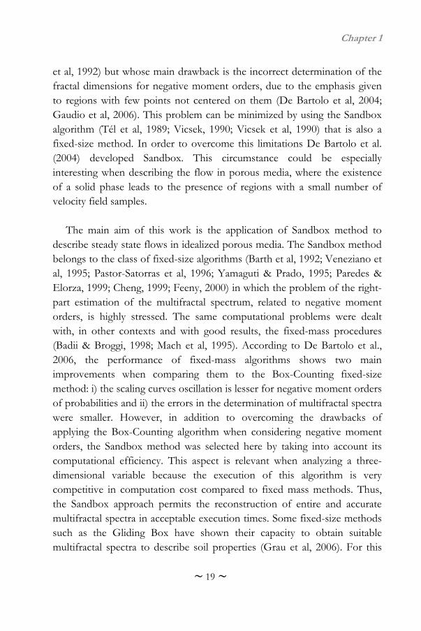
et al, 1992) but whose main drawback is the incorrect determination of the fractal dimensions for negative moment orders, due to the emphasis given to regions with few points not centered on them (De Bartolo et al, 2004; Gaudio et al, 2006). This problem can be minimized by using the Sandbox algorithm (Tél et al, 1989; Vicsek, 1990; Vicsek et al, 1990) that is also a fixed-size method. In order to overcome this limitations De Bartolo et al. (2004) developed Sandbox. This circumstance could be especially interesting when describing the flow in porous media, where the existence of a solid phase leads to the presence of regions with a small number of velocity field samples.

The main aim of this work is the application of Sandbox method to

describe steady state flows in idealized porous media. The Sandbox method belongs to the class of fixed-size algorithms (Barth et al, 1992; Veneziano et al, 1995; Pastor-Satorras et al, 1996; Yamaguti & Prado, 1995; Paredes & Elorza, 1999; Cheng, 1999; Feeny, 2000) in which the problem of the right-part estimation of the multifractal spectrum, related to negative moment orders, is highly stressed. The same computational problems were dealt with, in other contexts and with good results, the fixed-mass procedures (Badii & Broggi, 1998; Mach et al, 1995). According to De Bartolo et al., 2006, the performance of fixed-mass algorithms shows two main improvements when comparing them to the Box-Counting fixed-size method: i) the scaling curves oscillation is lesser for negative moment orders of probabilities and ii) the errors in the determination of multifractal spectra were smaller. However, in addition to overcoming the drawbacks of applying the Box-Counting algorithm when considering negative moment orders, the Sandbox method was selected here by taking into account its computational efficiency. This aspect is relevant when analyzing a three-dimensional variable because the execution of this algorithm is very competitive in computation cost compared to fixed mass methods. Thus, the Sandbox approach permits the reconstruction of entire and accurate multifractal spectra in acceptable execution times. Some fixed-size methods such as the Gliding Box have shown their capacity to obtain suitable multifractal spectra to describe soil properties (Grau et al, 2006). For this

Chapter 1

~ 20 ~ 

 

reason, the peculiarity of the present work lies in the first time application of the Sandbox method to describe flows in porous media.

The three-dimensional velocity fields were simulated with the lattice

Bathnagar-Gross-Krook (BGK) model (Succi, 2001), an improved version of the lattice Boltzmann model. These porous media were generated by using the method proposed by Rappoldt and Crawford (Rappoldt & Crawford, 1999).

2. Methods

2.1. The lattice Bathnagar-Gross-Krook (BGK) model

In the lattice BGK model (Chen et al, 1992; Qian et al, 1992), the fluid particles move in a regular lattice where each node is linked to its neighbours following a vicinity model that is chosen depending on the complexity of the phenomenon to be simulated. The vicinity model d3Q19 is frequently used to calculate the flow velocity field in three dimensions (Succi, 2001), in which d = 3 means the number of dimensions and Q = 19 denotes the number of particles considered, in this case eighteen moving particles and one at rest.

The equation of the lattice BGK model for a node r at time t, is

eq1 1( , ) ( , ) 1 ( , )k k k kf t t t f t f tr c r r

(1)

where the independent variable kf varies continuously between 0 and 1

according to the Boltzmann molecular chaos hypothesis and represents the probability of finding a fluid particle in a link k that connects a node with

Chapter 1

~ 21 ~ 

 

one of its neighbours. The interactions of the particles keep up the mass and momentum ((Rothman & Zaleski, 1997; Chopard & Droz, 1998).

The vector ck stands for the velocity of a fluid particle in the link k and it

is defined by Eq. (2).

(0, 0, 0) ( 0),

( 1,0,0), (0, 1,0), (0, 0, 1), ( 1 to 6),

( 1, 1,0), ( 1, 0, 1), (0, 1, 1), ( 7 to 18) k

k

c c c k

c c c k

c

(2)

where c r t , with r being the length of the lattice spacing.

eq

kf is the local equilibrium function and is the relaxation time

parameter that represents the difference between kf and eqkf . The right

hand side of Eq. (1) has been obtained from a Taylor series expansion

under the assumption that kf is near to eqkf , implying that has to be

small enough to neglect the high order terms of the expansion. Using the Chapman–Enskog expansion, it is mathematically demonstrable that Eq. (1) can recover the Navier-Stokes equations to the second order of accuracy

(Succi, 2001; Chopard & Droz, 1998) if eqkf is chosen in the following way:

2

eq

2 2 2

eq

2

11 , [1, 1]

2 2

1 , 02

k kk k

s s s

k k

s

c v c v v vf b k Q

c c c

v vf b k

c

(3)

 

where the Einstein summation convention has been adopted. v and ck are

the components of the vectors v and ck in the dimension ( = x, y, z, the spatial coordinates). bk are weighting factors associated with the lattice directions and the parameter cs, known as the speed of sound, is selected

Chapter 1

~ 22 ~ 

 

according to the vicinity model chosen. For the d3Q19 neighborhood model

it is found that 2 2 3sc c , b0 = 1/3, b1-6 = 1/18 and b7-18 = 1/36. The fluid

density and velocity v are deduced fromkf according to

1

0

1

1

( , ) ( , )

( , )( , )

( , )

Q

kk

Q

k kk

t f t

f tt

t

r r

r cv r

r

(4)

and the kinematic viscosity, , is defined as

22 1

2s

rc

t (5)

Thus, the relaxation time should be greater than 1/2 to ensure positive

values for . In this work, it is assumed that 1r x y z lattice

unit (l.u.) and t = 1 time-step (ts) as is frequently adopted in lattice model simulations (Succi, 2001). The conversion rules between the magnitudes used in the lattice BGK model and their real physical values can be obtained

from realt t t , realr r r , ( ) realv r t v and 2( ) real r t ,

where the scale factors r and t are expressed in SI units.

2.2. Features of the numerical simulations

In all the cases, the three-dimensional computational domain was represented by a cube of L = 64 l.u. in side length. The idealised porous media were generated by using the random fractal lattice proposed by Rappoldt and Crawford (Rappoldt & Crawford, 1999), in which the

porosity, , is determined by 1 p , where p is the probability that a

node comprises solid phase and 1 is the number of levels of recursion,

Chapter 1

~ 23 ~ 

 

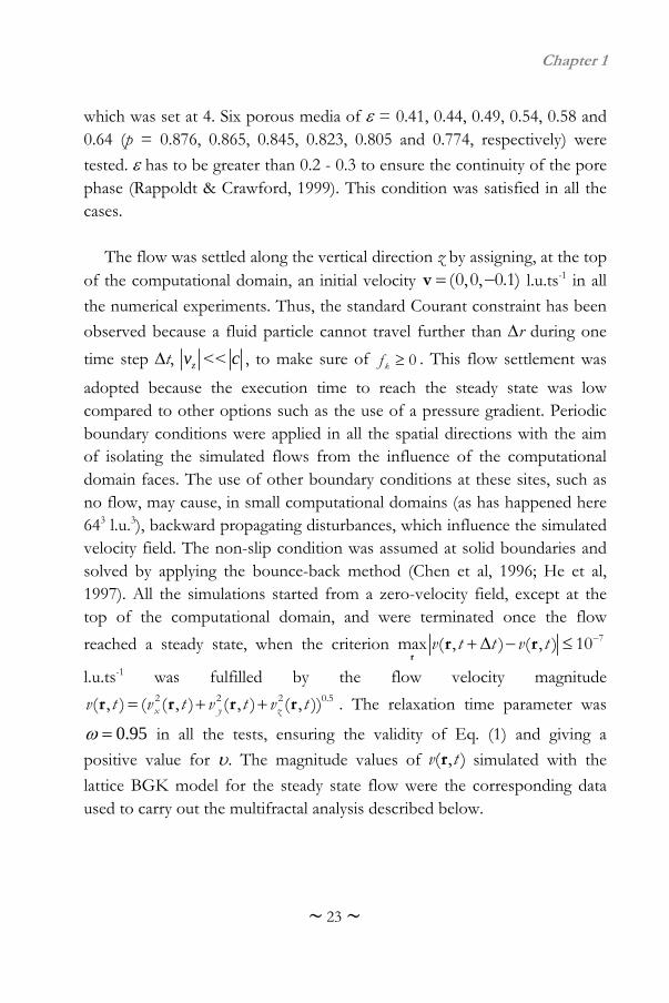
which was set at 4. Six porous media of = 0.41, 0.44, 0.49, 0.54, 0.58 and 0.64 (p = 0.876, 0.865, 0.845, 0.823, 0.805 and 0.774, respectively) were

tested. has to be greater than 0.2 - 0.3 to ensure the continuity of the pore phase (Rappoldt & Crawford, 1999). This condition was satisfied in all the cases.

The flow was settled along the vertical direction z by assigning, at the top

of the computational domain, an initial velocity (0,0, 0.1)v l.u.ts-1 in all

the numerical experiments. Thus, the standard Courant constraint has been

observed because a fluid particle cannot travel further than r during one

time step t, zv << c , to make sure of 0kf . This flow settlement was

adopted because the execution time to reach the steady state was low compared to other options such as the use of a pressure gradient. Periodic boundary conditions were applied in all the spatial directions with the aim of isolating the simulated flows from the influence of the computational domain faces. The use of other boundary conditions at these sites, such as no flow, may cause, in small computational domains (as has happened here 643 l.u.3), backward propagating disturbances, which influence the simulated velocity field. The non-slip condition was assumed at solid boundaries and solved by applying the bounce-back method (Chen et al, 1996; He et al, 1997). All the simulations started from a zero-velocity field, except at the top of the computational domain, and were terminated once the flow

reached a steady state, when the criterion 7max ( , ) ( , ) 10v t t v tr

r r

l.u.ts-1 was fulfilled by the flow velocity magnitude

2 2 2 0.5( , ) ( ( , ) ( , ) ( , ))x y zv t v t v t v tr r r r . The relaxation time parameter was

0.95 in all the tests, ensuring the validity of Eq. (1) and giving a

positive value for . The magnitude values of ( , )v tr simulated with the

lattice BGK model for the steady state flow were the corresponding data used to carry out the multifractal analysis described below.

Chapter 1

~ 24 ~ 

 

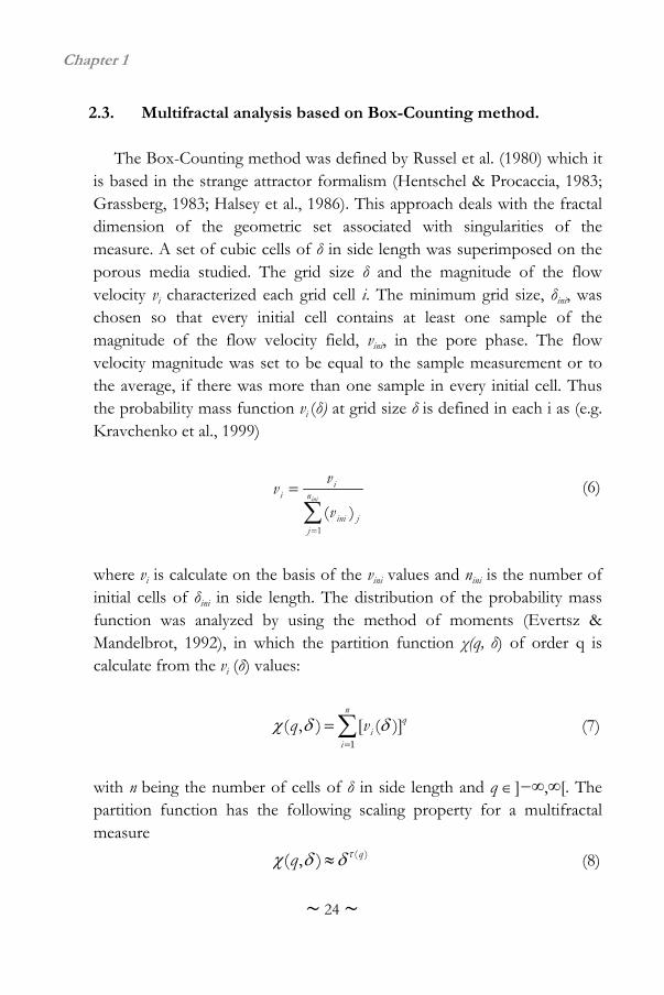
2.3. Multifractal analysis based on Box-Counting method. The Box-Counting method was defined by Russel et al. (1980) which it

is based in the strange attractor formalism (Hentschel & Procaccia, 1983; Grassberg, 1983; Halsey et al., 1986). This approach deals with the fractal dimension of the geometric set associated with singularities of the measure. A set of cubic cells of δ in side length was superimposed on the porous media studied. The grid size δ and the magnitude of the flow velocity vi characterized each grid cell i. The minimum grid size, δini, was chosen so that every initial cell contains at least one sample of the magnitude of the flow velocity field, vini, in the pore phase. The flow velocity magnitude was set to be equal to the sample measurement or to the average, if there was more than one sample in every initial cell. Thus the probability mass function vi (δ) at grid size δ is defined in each i as (e.g. Kravchenko et al., 1999)

1

( )ini

ii n

ini jj

vv

v

(6)

where vi is calculate on the basis of the vini values and nini is the number of initial cells of δini in side length. The distribution of the probability mass function was analyzed by using the method of moments (Evertsz & Mandelbrot, 1992), in which the partition function χ(q, δ) of order q is calculate from the vi (δ) values:

1

( , ) [ ( )]n

qi

i

q v (7)

with n being the number of cells of δ in side length and q ]−∞,∞[. The partition function has the following scaling property for a multifractal measure

( )( , ) qq (8)

Chapter 1

~ 25 ~ 

 

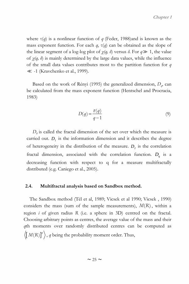
where τ(q) is a nonlinear function of q (Feder, 1988)and is known as the mass exponent function. For each q, τ(q) can be obtained as the slope of the linear segment of a log-log plot of χ(q, δ) versus δ. For q 1, the value of χ(q, δ) is mainly determined by the large data values, while the influence of the small data values contributes most to the partition function for q -1 (Kravchenko et al., 1999). Based on the work of Rényi (1995) the generalized dimension, Dq, can be calculated from the mass exponent function (Hentschel and Procracia, 1983)

( )

( )1

qD q

q (9)

D0 is called the fractal dimension of the set over which the measure is

carried out. 1D is the information dimension and it describes the degree

of heterogeneity in the distribution of the measure. 2D is the correlation

fractal dimension, associated with the correlation function. qD is a

decreasing function with respect to q for a measure multifractally distributed (e.g. Caniego et al., 2005).

2.4. Multifractal analysis based on Sandbox method.

The Sandbox method (Tél et al, 1989; Vicsek et al 1990; Vicsek , 1990) considers the mass (sum of the sample measurements), ( )M R , within a

region i of given radius R (i.e. a sphere in 3D) centred on the fractal. Choosing arbitrary points as centres, the average value of the mass and their qth moments over randomly distributed centres can be computed as

( )q

M R , q being the probability moment order. Thus,

Chapter 1

~ 26 ~ 

 

1 ( 1)

0 0

qq q D

i i

i

M M R

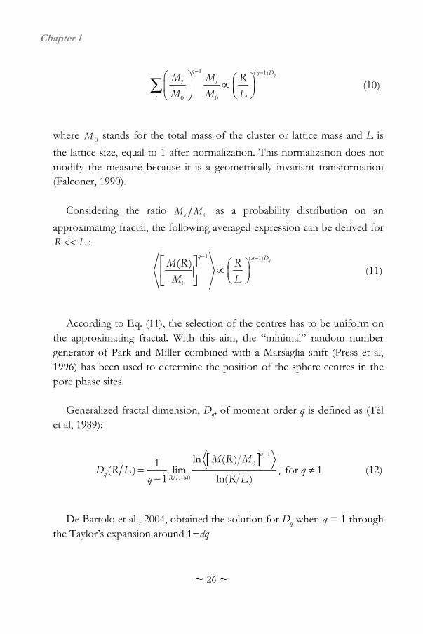
M M L (10)

 

where 0M stands for the total mass of the cluster or lattice mass and L is

the lattice size, equal to 1 after normalization. This normalization does not modify the measure because it is a geometrically invariant transformation (Falconer, 1990).

Considering the ratio 0iM M as a probability distribution on an

approximating fractal, the following averaged expression can be derived for R L :

1 ( 1)

0

( ) qq q D

M R R

M L

(11)

 

According to Eq. (11), the selection of the centres has to be uniform on the approximating fractal. With this aim, the “minimal” random number generator of Park and Miller combined with a Marsaglia shift (Press et al, 1996) has been used to determine the position of the sphere centres in the pore phase sites.

Generalized fractal dimension, Dq, of moment order q is defined as (Tél

et al, 1989):

1

0

0

ln ( )1( ) lim , for 1

1 ln( )

q

qR L

M R MD R L q

q R L (12)

 

De Bartolo et al., 2004, obtained the solution for Dq when q = 1 through the Taylor’s expansion around 1+dq

Chapter 1

~ 27 ~ 

 

01 0

ln ( )( ) lim

ln( )R L

M R MD R L

R L (13)

 

Generalized dimensions can be obtained through the least squares linear

regression as the slope of the scaling curves 1

0ln ( )q

M R M versus

ln( )R L for q ≠ 1 and 0ln ( )M R M versus ln( )R L for q = 1,

between ln( )lowerR L and ln( )upperR L , ( )lowerR L and ( )upperR L being the

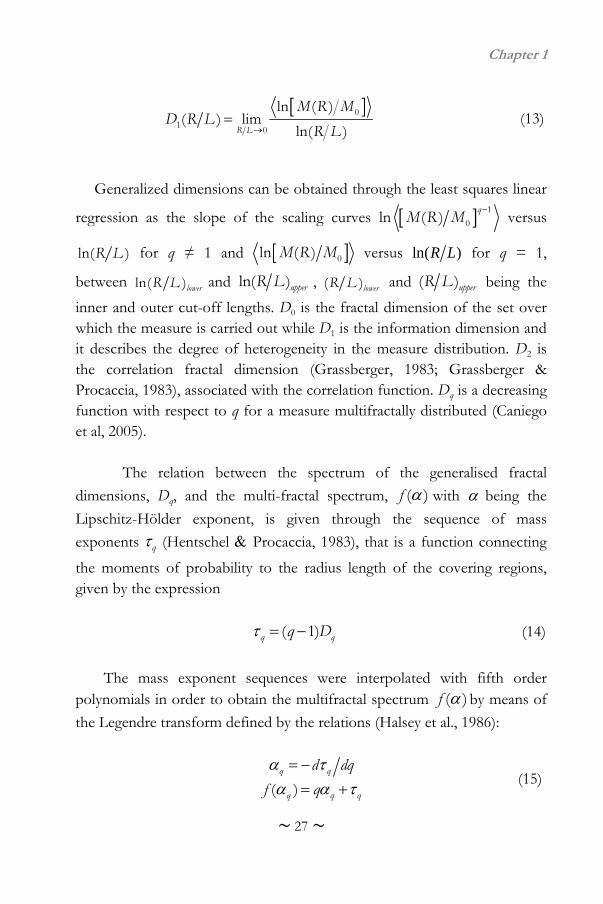
inner and outer cut-off lengths. D0 is the fractal dimension of the set over which the measure is carried out while D1 is the information dimension and it describes the degree of heterogeneity in the measure distribution. D2 is the correlation fractal dimension (Grassberger, 1983; Grassberger & Procaccia, 1983), associated with the correlation function. Dq is a decreasing function with respect to q for a measure multifractally distributed (Caniego et al, 2005).

The relation between the spectrum of the generalised fractal

dimensions, Dq, and the multi-fractal spectrum, ( )f with being the

Lipschitz-Hölder exponent, is given through the sequence of mass

exponents q (Hentschel Procaccia, 1983), that is a function connecting

the moments of probability to the radius length of the covering regions, given by the expression

( 1)q qq D (14)

The mass exponent sequences were interpolated with fifth order

polynomials in order to obtain the multifractal spectrum ( )f by means of

the Legendre transform defined by the relations (Halsey et al., 1986):

( )

q q

q q q

d dq

f q (15)

Chapter 1

~ 28 ~ 

 

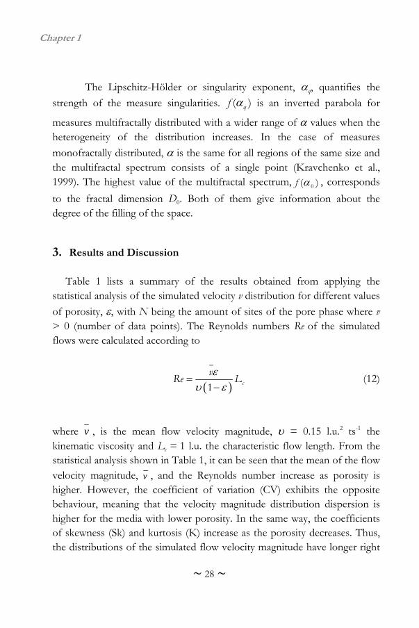
The Lipschitz-Hölder or singularity exponent, q, quantifies the

strength of the measure singularities. ( )qf is an inverted parabola for

measures multifractally distributed with a wider range of values when the heterogeneity of the distribution increases. In the case of measures

monofractally distributed, is the same for all regions of the same size and the multifractal spectrum consists of a single point (Kravchenko et al., 1999). The highest value of the multifractal spectrum, 0( )f , corresponds

to the fractal dimension D0. Both of them give information about the degree of the filling of the space.

3. Results and Discussion

Table 1 lists a summary of the results obtained from applying the statistical analysis of the simulated velocity v distribution for different values

of porosity, , with N being the amount of sites of the pore phase where v > 0 (number of data points). The Reynolds numbers Re of the simulated flows were calculated according to

1 c

vRe L

(12)

 

where v , is the mean flow velocity magnitude, = 0.15 l.u.2 ts-1 the kinematic viscosity and Lc = 1 l.u. the characteristic flow length. From the statistical analysis shown in Table 1, it can be seen that the mean of the flow velocity magnitude, v , and the Reynolds number increase as porosity is higher. However, the coefficient of variation (CV) exhibits the opposite behaviour, meaning that the velocity magnitude distribution dispersion is higher for the media with lower porosity. In the same way, the coefficients of skewness (Sk) and kurtosis (K) increase as the porosity decreases. Thus, the distributions of the simulated flow velocity magnitude have longer right

Chapter 1

~ 29 ~ 

 

tails and sharper peaks around the mean when the lowest values of porosity are considered.

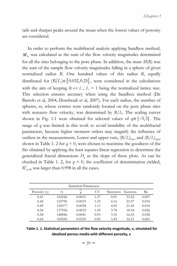
In order to perform the multifractal analysis applying Sandbox method,

0M was calculated as the sum of the flow velocity magnitudes determined

for all the sites belonging to the pore phase. In addition, the mass M(R) was the sum of the sample flow velocity magnitudes falling in a sphere of given normalized radius R. One hundred values of this radius R, equally

distributed for ( ) 0.032,0.25R L , were considered in the calculations

with the aim of keeping R L , L = 1 being the normalized lattice size. This selection ensures accuracy when using the Sandbox method (De Bartolo et al, 2004; Dombradi et al, 2007). For each radius, the number of spheres, ns, whose centres were randomly located on the pore phase sites with nonzero flow velocity, was determined by R/L. The scaling curves shown in Fig. 1.1 were obtained for selected values of [ 5,5]q . The

range of q was limited in this work to avoid instability of the multifractal parameters, because higher moment orders may magnify the influence of outliers in the measurements. Lower and upper cuts, (R/L)lower and (R/L)upper shown in Table 1. 2 for q = 0, were chosen to maximise the goodness of the fits obtained by applying the least squares linear regression to determine the generalized fractal dimensions Dq as the slope of these plots. As can be checked in Table 1. 2, for q = 0, the coefficient of determination yielded, R2

q=0, was larger than 0.998 in all the cases.

Porosity (ε) N CV Skewness Kurtosis Re0.41 102526 0.0015 1.57 4.91 33.62 0.0070.44 110796 0.0019 1.25 4.16 23.27 0.0100.49 124577 0.0028 1.11 4.05 21.45 0.0180.54 137956 0.0033 1.05 3.78 18.34 0.0260.58 148846 0.0041 0.93 3.55 16.25 0.0380.64 165045 0.0550 0.85 3.45 16.21 0.065

Statistical Parameters

v

 

 Table 1. 1. Statistical parameters of the flow velocity magnitude, v, simulated for 

idealized porous media with different porosity, ε 

Chapter 1

~ 30 ~ 

 

Figure 1. 1. Scaling curves of the flow velocity magnitude distribution in idealisedmedia with different porosity ε obtained from the application of the Sandboxmethod by considering selected values of the order q.

Chapter 1

~ 31 ~ 

 

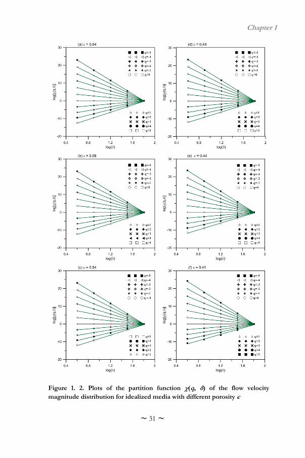
Figure 1. 2. Plots of the partition function χ(q, δ) of the flow velocitymagnitude distribution for idealized media with different porosity є

Chapter 1

~ 32 ~ 

 

The minimum grid size selected to carry out the Box-Counting method was δini=4 l.u. Fig. 1. 2 shows the plot of the partition function of v, χ(q, δ), versus the grid size, that ranges from δ = δini = 4 l.u to δ = 64 l.u., for different values of ε. For all the statistical orders tested, q=-5 to 5, the log transformated χ(q, δ) are straight lines meaning that the estimation of τ(q) as theirs slopes can be trusted. The coefficient of determination, R2, was larger than 0,99in all the fits (Fig. 1. 2).

The mass exponents functions of v, τ(q), were obtained from the slopes

of these fits and are plotted in Fig. 1. 3. Note that the slopes of the τ(q) curves for q < 0 are different from that of q > 0 for all the porosity values tested, indicating that τ(q) curves are convex and increased in convexity as the porosity decreases.

Porosity ( ε) D 0 D 1 D 2 D 0 D 1 D 2 (R/L) lower (R/L) upper R 2q=0

0.41 3 2.7837 2.5548 2.8960 2.8040 2.6330 0.0540 0.250 0.998670.44 3 2.8398 2.6621 2.8530 2.7760 2.6510 0.0630 0.250 0.999030.49 3 2.8664 2.7109 2.8520 2.7930 2.7020 0.0630 0.250 0.998390.54 3 2.8738 2.7279 2.8470 2.7870 2.6990 0.0630 0.250 0.999110.58 3 2.8959 2.7743 2.8220 2.7730 2.7020 0.0570 0.250 0.999070.64 3 2.9100 2.8041 2.8400 2.7960 2.7390 0.0610 0.250 0.99909

Box-Counting Method Sandbox Method

Multifractal Parameters

 Table 1. 2. Box-Counting and Sandbox multifractal parameters Rényi spectra. 

Figure 1. 3. Mass exponent of the flow velocity magnitude obtained from Box-Counting method.

Chapter 1

~ 33 ~ 

 

 

Figure 1. 4. The generalized fractal dimensions spectra of the flow velocitymagnitude distribution estimated with the Sandbox and Box-Countingmethods for idealized media with different porosity ε. Bars represent thestandard errors.

Chapter 1

~ 34 ~ 

 

Figure 1. 4 shows the spectra of the generalized fractal dimensions

obtained with Sandbox and Box-Counting methods. Dq is a decreasing function in all the cases, with D0>D1>D2 as can be checked in Table 1. 2, denoting a multiscaling behaviour. According to the lengths of the error bars shown in Fig. 1. 4, the estimation of Dq by applying the Sandbox and Box-Counting procedures can be trusted. For q < 0, the error in the estimation of Dq with Box-Counting procedure is lower as the porosity increases. However, the error values obtained for the same situation with Sandbox method do not display any relevant variations when the porosity varies. Figure 1. 5 shows the average relative differences between both methods and it can be verified that they increase as q is more negative. In addition, these differences for q < 0 are higher compared to the case of q > 0. This dissimilarity can be explained because Sandbox method solves the border effect problem caused by the presence of almost empty cubic cells containing few points not centred on them.

Figure 1. 5. Comparison of the generalized fractaldimensions spectra, Dq, estimated with the Sandboxmethod and Box-Counting procedures.

Chapter 1

~ 35 ~ 

 

Differences were found the spectra of the generalized fractal dimensions determined with Box-Counting and Sandbox methods. Higher values for Dq were obtained with Box-Counting method, especially when considering q < 0 (Figs. 1.4 and 1.5). This circumstance is a consequence of the emphasis given in the Box-Counting algorithm to regions with few data. In addition, Sandbox method reduces the shape effect of pore network, due to the overlap of the spheres centred on the fractal. Although these differences in values continue for q > 0, they are much lower.

From the spectra of the generalized fractal dimensions obtained with

Sandbox method, it can be verified that D0 < 3 in all the cases (Table 1. 2). This fact is in contrast with D0 = 3 found for the analysis performed on the same flows considered here through the application of Box-Counting procedure. Thus, the sphere centres were randomly located on the pore phase sites with nonzero flow velocity magnitude when applying Sandbox method. In the same way, a set of different grids with non-overlapping cubic cells of different size lengths is superimposed on the porous media studied when it is used Box-Counting method. The minimum grid size is chosen so that every initial box contains at least one sample of nonzero flow velocity magnitude field in the pore phase. However, as a consequence of using overlapped spheres centred on the fractal, the determination of fractal dimensions by the Sandbox algorithm is more suitable. Thus, the values obtained for Dq with the Sandbox method demonstrate that flows cannot fill the 3D domain where they take place due to the influence of the pore phase geometry. This fact can be noted in Fig. 1. 6 that corresponds to two cross-sections of the three-dimensional velocity fields simulated by

using the lattice BGK model, when considering porous media of = 0.41

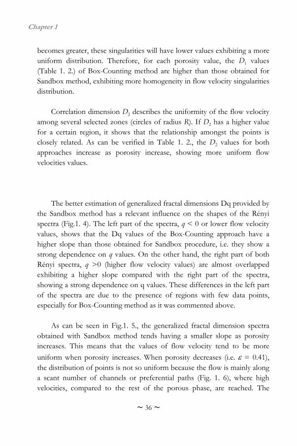
and = 0.64. In accordance with Davis et al. (1994), the information dimension D1

provides a measure of the degree of heterogeneity in the spatial distribution of a variable. In addition, D1 characterizes the distribution and intensity of singularities with respect to the mean. If D1 is lower, the distribution of singularities in the flow velocity will be sparse. On the contrary, if D1

Chapter 1

~ 36 ~ 

 

becomes greater, these singularities will have lower values exhibiting a more uniform distribution. Therefore, for each porosity value, the D1 values (Table 1. 2.) of Box-Counting method are higher than those obtained for Sandbox method, exhibiting more homogeneity in flow velocity singularities distribution.

Correlation dimension D2 describes the uniformity of the flow velocity

among several selected zones (circles of radius R). If D2 has a higher value for a certain region, it shows that the relationship amongst the points is closely related. As can be verified in Table 1. 2., the D2 values for both approaches increase as porosity increase, showing more uniform flow velocities values.

The better estimation of generalized fractal dimensions Dq provided by

the Sandbox method has a relevant influence on the shapes of the Rényi spectra (Fig.1. 4). The left part of the spectra, q < 0 or lower flow velocity values, shows that the Dq values of the Box-Counting approach have a higher slope than those obtained for Sandbox procedure, i.e. they show a strong dependence on q values. On the other hand, the right part of both Rényi spectra, q >0 (higher flow velocity values) are almost overlapped exhibiting a higher slope compared with the right part of the spectra, showing a strong dependence on q values. These differences in the left part of the spectra are due to the presence of regions with few data points, especially for Box-Counting method as it was commented above.

As can be seen in Fig.1. 5., the generalized fractal dimension spectra

obtained with Sandbox method tends having a smaller slope as porosity increases. This means that the values of flow velocity tend to be more

uniform when porosity increases. When porosity decreases (i.e. = 0.41), the distribution of points is not so uniform because the flow is mainly along a scant number of channels or preferential paths (Fig. 1. 6), where high velocities, compared to the rest of the porous phase, are reached. The

Chapter 1

~ 37 ~ 

 

description provided by the analysis carried out with Sandbox method improves the results obtained with Box-Counting procedure because the multifractal spectra estimated by the latter do not show, in such an obvious way, the influence of porous media structure on flow velocity distribution.

Figure 1. 6. Cross-sections of the flow velocity magnitude, expressed in lattice units

(l.u.) by time step (ts), for idealised media with porosities (a) = 0.41 and (b) = 0.64.The black zones correspond to the solid phase of the porous media and the whitearrows indicate the flow direction.

Chapter 1

~ 38 ~ 

 

4. Conclusions Sandbox method has shown to be an efficient algorithm to describe the

flow velocity distribution in porous media compared with Box-Counting method. Sandbox method shows that flow velocity values tend to be more uniform when porosity increases. However, this fact is not detected by Box-Counting method, improving Sandbox approach the results obtained for this study.

The results obtained from generalized fractal dimensions spectra show

the multifractal nature of flow velocity in porous media. The determination of scale-dependent variability of the flows in porous media becomes essential to their description (Wnag et al, 2006). Highly heterogeneous transport phenomena have been observed from field experiments and the flow heterogeneity increases with the measurement scale (Koirala et al, 2008). For this reason, it is desirable to describe flow and transport phenomena in large scales from observations at smaller scales. In line with the results obtained here, the combination of lattice BGK model simulations with multifractal analysis introduced in this work can be an alternative to face this challenge.

This work can be considered as being the first step in a research line that

will combine numerical simulations of flows taking place in real porous media, whose geometry can be obtained by 3D tomography or other geometric modelling, and multifractal analysis. The information provided will help to improve the quality of future models developed by researchers to describe flows in porous media with environmental relevance such as involving soil pollutants transport.

Chapter 1

~ 39 ~ 

 

References

Badii, R. & Broggi, G. (1988). Measurement of the dimension spectrum f(α) - fixed-mass approach. Phys. Lett. A, 131, 339 – 343.

Barth, A., Baumann, G., & Nonnenmacher, T.F. (1992). Measuring Rényi

dimensions by a modified box algorithm. J. Phys. A-Math. Theor., 25 381 – 391.

Bird, N., Diaz, M.C., Saa, A. &. Tarquis, A.M. (2006). Fractal and

multifractal analysis of pore-scale images of soil. J. Hydrol., 322, 211 – 219.

Caniego, F.J., Espejo, R., Martin, M.A. & San Jose, F. (2005). Multifractal

scaling of soil spatial variability. Ecol. Model. 182, 291 – 303. Chen, S., Martinez, D., & Mei, R. (1996). On boundary conditions in lattice

Boltzmann methods. Phys. Fluids, 8, 2527 – 2536. Chen, S., Wang, Z., Shan, X. & Doolen, G. (1992). Lattice Boltzmann

computational fluid dynamics in three dimensions. J. Stat. Phys., 68, 379 – 400.

Cheng, Q. (1999). The gliding box method for multifractal modelling.

Comp. Geosci., 25, 1073 – 1079. Chopard, B., & Droz, M. (1998). Cellular Automata Modeling of Physical

Systems. Cambridge: Cambridge University Press. Cihan, A., Sukop, M., Tyner, J.S., Perfect, E., & Huang, H. (2009).

Analytical predictions and lattice Boltzmann simulations of intrinsic permeability for mass fractal porous media. Vadose Zone J., 8, 187 – 196.

Chapter 1

~ 40 ~ 

 

Davis, A., Marshak, A., Wiscombe, W., &, Cahalan, R. (1994). Multifractal characterization of non stationarity and intermitency in geophysical fields: observed, retrieved or simulated. J. Geophys. Res., 99, 8055 – 8072.

De Bartolo, S.G., Gaudio, R. & Gabriele, S. (2004). Multifractal analysis of

river networks: Sandbox approach. Water Resour. Res., 40, W02201, doi:10.1029/2003WR002760.

De Bartolo, S.G., Primavera, L., Gaudio, R., D'Ippolito, A., & Veltri, M.

(2006). Fixed-mass multifractal analysis of river networks and braided channels. Phys. Rev. E., 74, 026101, doi:10.1103/PhysRevE.74.026101.

Dombradi, E., Timár, G., Bada, G., Cloetingh, S. & Horváth, F. (2007).

Fractal dimension estimations of drainage network in the Carpathian-Pannonian system. Glob. Planet. Change, 58, 197 – 213.

Evertsz, C.J.G., & Mandelbrot, B.B. (1992). Multifractal measures. In:

Chaos and Fractals. New York : Springer-Verlag. Falconer, K.J. (1990). Fractal Geometry: Mathematical Foundations and

Applications. New York: John Wiley, Hoboken. Feder, J. (1998). Fractals. New York: Plenum. Feeny, B.F. (2000). Fast multifractal analysis by recursive box covering. Int.

J. Bifurcation Chaos, 10, 2277 – 2287. Gaudio, R., De Bartolo, S.G., Primavera, L., Gabriele, S. & Veltri, M.

(2006). Lithologic control on the multifractal spectrum of river networks, J. Hydrol., 327, 365 – 375.

Giménez, D., Rawls, W.J., & Lauren, J.G. (1999). Scaling properties of

saturated hydraulic conductivity in soil. Geoderma 88, 205 – 220.

Chapter 1

~ 41 ~ 

 

Grassberger, P. (1983). Generalized dimensions of strange attractors.

Physical Review Letters, 97(6), 227–230. Grassberger, P., & Procaccia, I. (1983). Characterization of strange

attractors. Physical Review Letters, 50(5), 346–349. Grau, J., Mendez, V., Tarquis, A.M., Diaz, M.C. & Saa, A. (2006).

Comparison of gliding box and box-counting methods in soil image analysis. Geoderma, 134, 349 – 359.

Grout, H., Tarquis, A.M. & Wiesner, M.R. (1998). Multifractal analysis of

particle size distributions in soil. Environ. Sci. Technol., 39, 1176 – 1182.

Halsey, T.C., Jensen, M.H., Kadanoff, L.P., Procaccia, I., & Shraiman, B.I.

(1986). Fractal measures and their singularities: the characterization of strange sets. Phys. Rev. A, 33, 1141 – 1151.

He, X.Y., Zou, Q.S., Luo, L.S., & Dembo, M. (1997). Analytic solutions of

simple flows and analysis of nonslip boundary conditions for the lattice Boltzmann BGK model. J. Stat. Phys., 87, 115 – 136.

Hentschel, H.G.E. & Procaccia, I., 1983. The infinite number of generalized

dimensions of fractals and strange attractors. Physica D, 8, 435 – 444. Islam, J., Singhal, N. & O'Sullivan, M. (2001). Modeling biogeochemical

processes in leachate-contaminated soils. A review, Transp. Porous Media, 43, 407 – 440.

Koirala, S.R., Perfect, E., Gentry, R.W. & Kim, J.W. (2008). Effective

saturated hydraulic conductivity of two-dimensional random multifractal fields. Water Resour. Res., 44, W08410, doi:10.1029/2007WR006199.

Chapter 1

~ 42 ~ 

 

Kravchenko, A.N., Boast, C.W., & Bullock, D.G. (1999). Multifractal

analysis of soil spatial variability. Agron. J., 91, 1033 – 1041. Kravchenko, A.N., Martin, M.A., Smucker, A.J.M., & Rivers, M.L. (2009).

Limitations in determining multifractal spectra from pore–solid soil aggregate images. Vadose Zone J., 8, 220 – 226.

Lehmann, P., Berchtold, M., Ahrenholz, B., Tolke, J., Kaestner, A.,

Krafczyk, M., Fluhler, H. & Kunsch, H.R. (2008). Impact of geometrical properties on permeability and fluid phase distribution in porous media. Adv. Water Resour., 31, 1188 – 1204.

Liu, H.H., & Molz, F.J. (1997). Multifractal analyses of hydraulic

conductivity distributions. Water Resour. Res., 33, 2483 – 2488. Mach, J., Mas, F. & Sagues, F. (1995). Two representations in multifractal

analysis. J. Phys. A-Math. Theor, 28, 5607 – 5622. Mandelbrot, B.B. (1982). The Fractal Geometry of Nature. New York:

W.H. Freeman. Martin, M.A., & Taguas, F.J. (1998). Fractal modelling, characterization and

simulation of particle-size distributions in soil. Proc. R. Soc. A-Math. Phys. Eng. Sci, 454, 1457 – 1468.

Martys, N., & Chen, H. (1996). Simulation of multicomponent fluids in

complex three-dimensional geometries by the lattice Boltzmann method. Phys. Rev. E, 53, 743 – 750.

Meisel, L.V., Johnson, M. & Cote, P.J. (1992). Box-counting multifractal

analysis. Phys. Rev. A, 45, 6989 – 6996.

Chapter 1

~ 43 ~ 

 

Montero, E. (2005). Rényi dimensions analysis of soil particle-size distributions. Ecol. Model., 182, 305 – 315.

Muller, J., Huseby, O.K., & Saucie, A. (1995). Influence of multifractal scaling of pore geometry on permeabilities of sedimentary rocks. Chaos Soliton. Fract., 5, 1485 – 1492.

Paredes, C., & Elorza, F.J. (1999). Fractal and multifractal analysis of

fractured geological media: surface-subsurface correlation. Comput. Geosci. 25, 1081 – 1096.

Pastor-Satorras, R., & Riedi, R. (1996). Numerical estimates of the

generalized dimensions of the Hénon attractor for negative q. J. Phys. A-Math. Theor., 29, L391 – L398.

Perfect, E., Gentry, R.W., Sukop, M.C. & Lawson, J.E. (2006). Multifractal

Sierpinski carpets: Theory and application to upscaling effective saturated hydraulic conductivity. Geoderma, 134, 240 – 252.

Posadas, A.N.D., Giménez, D., Bittelli, M., Vaz, C.M.P., & Flury, M. (2001).

Multifractal characterization of soil particle-size distributions. Soil Sci. Soc. Am. J., 65, 1361 – 1367.

Posadas, A.N.D., Giménez, D., Quiroz, R., & Protz, R. (2003). Multifractal

characterization of soil pore systems. Soil Sci. Soc. Am. J. 67, 1361 – 1369.

Press, W.H., Teukolsky, S.A., Vetterling, W.T. & Flannery, B.P. (1996).

Fortran Numerical Recipes: The Art of Parallel Scientific Computing. Cambridge: Cambridge University Press.

Qian, Y.H., D’Humieres, D., & Lallemand, P. (1992). Lattice BGK models

for Navier-Stokes equation. Europhys. Lett., 17, 479 – 484.

Chapter 1

~ 44 ~ 

 

Rappoldt, C., & Crawford, J.W. (1999). The distribution of anoxic volume in a fractal model of soil. Geoderma, 88, 329 – 347.

Rényi, A. (1970). Probability Theory. New York: American Elsevier

Publishing Company. Rinck-Pfeiffer, S., Ragusa, S., Sztajnbok, P. & Vandevelde, T. (2000).

Interrelationships between biological, chemical, and physical processes as an analog to clogging in aquifer storage and recovery (ASR) wells. Water Res., 34, 2110 – 2118.

Rothman, D.H., & Zaleski, S. (1997). Lattice-Gas Cellular Automata. Simple

Models of Complex Hydrodynamics. Cambridge: Cambridge University Press.

Russel, D., Hanson, J., & Ott, E. (1980). Dimension of strange attractors.

Phys. Rev. Lett., 45, 1175 – 1178. Succi, S. (2001). The Lattice Boltzmann Equation for Fluid Dynamics and

Beyond. Numerical Mathematics and Scientific Computation. Oxford: Oxford University Press.

Tél, T. Fülöp, Á, & Vicsek, T. (1989). Determination of fractal dimensions

for geometrical multifractals. Physica A, 159, 155 – 166. Thullner, M., Van Cappellen, P. & Regnier, P. (2005). Modeling the impact

of microbial activity on redox dynamics in porous media. Geochim. Cosmochim, 69, 5005 – 5019.

Veneziano, D., & Essiam, A.K. (2003). Flow through porous media with

multifractal hydraulic conductivity. Water Resour. Res., 39, 1166, doi:10.1029/2001WR001018.

Chapter 1

~ 45 ~ 

 

Veneziano, D., Moglen, G.E. & Bras, R.L. (1995). Multifractal analysis: pitfalls of standard procedures and alternatives. Phys. Rev. E, 52, 387 – 1398.

Vicsek, T. (1990). Mass multifractals. Physica A, 168, 490 – 497. Vicsek, T. Family, F. & Meakin, P. (1990). Multifractal geometry of

diffusion-limited aggregates. Europhys. Lett., 12, 217 – 222. Wang, K., Zhang, R., & Hiroshi, Y. (2006). Characterizing heterogeneity of

soil water flow by dye infiltration experiments. J. Hydrol., 328, 559 – 571.

Yamaguti, M., & Prado, C.P.C. (1995). A direct calculation of the spectrum

of singularities f(α) of multifractals. Phys. Lett. A, 206, 318 – 322. Yamaguti, M., & Prado, C.P.C. (1997). Smart covering for a box-counting

algorithm. Phys. Rev. E, 55, 7726 – 7732. Zhang, X.X., Deeks, L.K., Bengough, A.G., Crawford, J.W., & Young, I.M.

(2005). Determination of soil hydraulic conductivity using lattice Boltzmann method and thin-section technique. J. Hydrol., 306, 59 – 70.

Chapter 1

~ 46 ~ 

 

 

~ 47 ~ 

 

Chapter 2

 

 

“Bottomless wonders spring from simple rules, repeated without end.”

Benoit Mandelbrot

(1924-2010) 

 

 

~ 48 ~ 

 

  

 

Chapter 2

~ 49 ~ 

 

Chapter 2. Multifractal

analysis of axial maps applied to the study of urban

morphology.

Abstract Street layout is an important element of urban morphology that informs on urban patterns influenced by city growing through the years under different planning regulations and different socio-economic contexts. It is assumed by several authors that urban morphology has a fractal or monofractal nature. However, not all the urban patterns can be considered as monofractal because of the presence of different morphologies. Therefore, a single fractal dimension may not always be enough to describe urban morphology. In this sense, a multifractal approach serves to tackle this problem by describing urban areas in terms of a set of fractal dimensions. With this aim in mind, two different neighbourhoods of the city of Cordoba, in Andalusia (Spain), are analyzed by using the Sandbox multifractal method and lacunarity. We analyze the street patterns represented by axial maps and obtained from the Space Syntax algorithm. The results suggest that the Rényi dimension spectrum is superior to a single fractal dimension to describe the urban morphology of Cordoba, given the presence of regular and irregular street layouts established under different planning and socio-economic regimes.

KEYWORDS: urban morphology; axial maps; multifractal analysis; Sandbox method; lacunarity

Chapter 2

~ 50 ~ 

 

1. Introduction Urban spaces are commonly defined by street layout, which is an

important component of urban morphology, as determined by the distribution of buildings on a certain site. Street patterns have been classified as irregular, radial-concentric, rectangular and grid (Dickinson, 1961); star, satellite, linear, rectangular grid, other grid, baroque network and lacework (Lynch, 1981); regular, concentric and irregular (DTLR & CABE, 2001); and by over 100 additional descriptors for streets outlines, including radial, grid, tree and linear (Marshall, 2005). City morphology is classified according to the way streets are arranged; over time, several urban morphologies in a major community are influenced by various planning regulations and socio-economic conditions. Urban morphology provides information about the structural characteristics of a city; it provides insight into the structural origins of and impacts of historical change on the chronological processes concerning construction and reconstruction of a city.

An understanding of urban morphology facilitates the projection of future growth in municipal site. Therefore, different scientific approaches have focused on the development of statistical models, such as the Geographical Information System (GIS)-based approach (Allen & Lu, 2003; Xiao et al., 2006), that can be used to estimate future urban growth and obtain information about city sustainability (Czerkauer-Yamu & Frankhauser, 2010; Van Diepen & Henk, 2003). By utilising graphic tools to quantify and define characteristics of urban morphology, Hillier and Hanson (1984) reproduce and simplify the spatial composition of a city by determining the minimum number of axial lines required to cover all areas of an urban lattice; this approach graphically and accurately represents street networks through axial maps. This procedure has been successfully applied to city modelling (Jiang & Claramunt, 2002), urban design (Jeong & Ban, 2011), spatial distribution of urban pollution (Croxford, 1996), prediction of human movement (Jiang, 2007) and road network analysis (Duan & Wang, 2009; Hu et al., 2009).

Chapter 2

~ 51 ~ 

 

Urban morphology has also been described by several authors as exhibiting a fractal nature (Batty & Longley, 1987, 1994; Batty, 2008; Benguigui et al., 2000; De Keersmaecker et al., 2003; Feng & Chen, 2010; Frankhauser, 1998). Based on this notion, the morphology of a city can be described by a single fractal dimension. Milne (1990) argues that not all landscapes are fractal due to their contemporary patterns because several past processes have individually influenced their complexity. Therefore, a single fractal dimension may not always sufficiently describe an urban area due to the presence of heterogeneous fractal properties, as Encarnação et al. (2012) suggests. The multifractal analysis proposed in this research solves this dilemma by obtaining generalised fractal dimensions, or Rényi spectra, to describe data. The research is a meaningful contribution to the study of urban patterns because the multifractal approach transforms irregular data into a compact form and amplifies small differences between variables (Folorunso et al., 1994). In addition, a multifractal framework exhibits a significant advantage over traditional methods through the integration of variability and scaling analyses (Stanley & Meakin, 1988; Kravchenko et al., 1999; Lee, 2002).

Multifractal analyses have been successfully applied to the study of

river network morphology with significant results (De Bartolo et al., 2000, 2004, 2006; Rinaldo et al., 1993). De Bartolo et al. (2004) has applied the Sandbox method to overcome limitations detected in the most frequently used multifractal fixed-sized algorithm, the Box-Counting algorithm (Mach et al., 1995), to describe river networks. River networks and streets have common properties such as hierarchy and critical self-organisation (Chen, 2009). Based on this context, this research proposes to describe urban patterns by using the multifractal Sandbox method. Apparently, it is the first study that characterises different urban areas to obtain a set of fractal dimensions. Two neighbourhoods in the city of Cordoba (Andalusia, southern Spain) are analysed. The street networks are defined by the Space Syntax algorithm (Hiller & Hanson, 1984). To complete the multifractal analysis, a lacunarity study is conducted. Lacunarity describes the texture appearance of an image, on different scales, based on the distribution of

Chapter 2

~ 52 ~ 

 

gaps or holes. It is applied to real data sets that may have a fractal or multifractal nature (Plotnick et al., 1996). This analysis is frequently utilised to develop urban spatial configurations (Alves Junior & Barros Filho, 2005; Amorim et al., 2009; Myint & Lam, 2005) and segregation; Wu Sui, 2001).

The paper is organised as follows: Section 2 introduces the Space

Syntax algorithm and the multifractal theory that is required to model and describe urban patterns. Section 3 details the study areas and discusses the main results of a multifractal analysis. Section 4 includes conclusions and recommendations for further research.

2. Combination of Axial Maps and Multifractal Analysis to Describe Urban Morphology

2.1. Axial Maps

Space Syntax is a set of tools that describes spatial configuration

through connectivity lines that cover all areas of a plane. This set of lines comprises an axial map (Peponis et al., 1998; Turner et al., 2005), which is one of the primary tools of Space Syntax. According to Turner (2006), an axial map is an abstraction of the space between buildings, which is depicted by straight lines and drawn according to a formal algorithm. The lines represent edges and intersections of lines represent junctions or connections between edges. Based on the algorithm, the axial map is the minimal set of axial lines that are linked in such a way that they completely cover the space.

Several authors have developed different computer programs for the

construction of axial maps based on the initial proposal of Hiller and Hanson (1984). Some programs have been implemented in GIS, such as Axman, which was created by Nick Dalton at University College in London (Major et al., 1997) and Axwoman, which was developed by Jiang et al. (1999). Both are used to draw axial lines with a computer and analyse axial

Chapter 2

~ 53 ~ 

 

maps of urban and interior spaces; the main difference between the programs is that Axman is a Mac-based application and Axwoman is a Windows-based application.

Other software have been designed to generate axial maps

automatically. Turner et al. (2005) introduced a universal-platform software, called Depthmap, to perform a set of spatial network analyses designed to explain social processes within a built environment. AxialGen, which was developed by Jiang and Liu (2009a), is a research prototype for automatically generating axial maps to demonstrate that axial lines constitute a true skeleton of an urban space. Although it is a good approximation of the axial map proposed by Hiller and Hanson (1984), this prototype has not been sufficiently tested.

This research, which follows the method proposed by Tuner et al.

(2005), extracts axial maps that successfully demonstrate and implement the algorithm proposed by Hiller and Hanson (1984) by obtaining accurate results with Depthmap. To translate formal language into algorithmic implementation, the definition of axial maps given by Hiller and Hanson (1984) was clarified and rewritten as “An axial map is the minimal set of lines such that the set taken together fully surveils the system and every axial line that may connect two otherwise unconnected lines is included”. To create the axial map, Tuner et al. (2005) establish two conditions: i) the reduction from the all-lines map to a unique minimal axial graph of the system and ii) the ability to surveil the entire system through axial lines and the preservation of topological rings.

Any possible axial lines are calculated from a map in which all streets

and blocks (polygons) are displayed. Every axial line is defined by joining two intervisible vertices. There are three different possibilities (Fig. 2.1): i) both of the vertices are convex, ii) one vertex is convex and one is concave or iii) both vertices are concave.

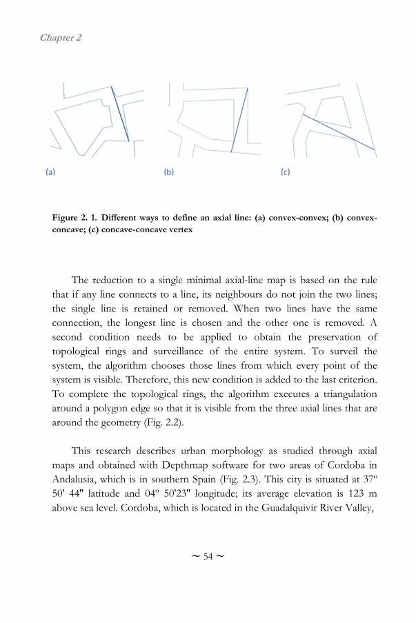
Chapter 2

~ 54 ~ 

 

 

Figure 2. 1.  Different ways to define an axial line: (a) convex-convex; (b) convex-concave; (c) concave-concave vertex 

The reduction to a single minimal axial-line map is based on the rule

that if any line connects to a line, its neighbours do not join the two lines; the single line is retained or removed. When two lines have the same connection, the longest line is chosen and the other one is removed. A second condition needs to be applied to obtain the preservation of topological rings and surveillance of the entire system. To surveil the system, the algorithm chooses those lines from which every point of the system is visible. Therefore, this new condition is added to the last criterion. To complete the topological rings, the algorithm executes a triangulation around a polygon edge so that it is visible from the three axial lines that are around the geometry (Fig. 2.2).

This research describes urban morphology as studied through axial

maps and obtained with Depthmap software for two areas of Cordoba in Andalusia, which is in southern Spain (Fig. 2.3). This city is situated at 37º 50' 44'' latitude and 04º 50'23'' longitude; its average elevation is 123 m above sea level. Cordoba, which is located in the Guadalquivir River Valley,

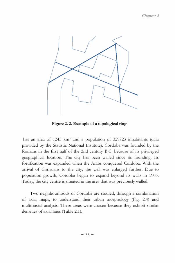
Chapter 2

~ 55 ~ 

 

has an area of 1245 km² and a population of 329723 inhabitants (data provided by the Statistic National Institute). Cordoba was founded by the Romans in the first half of the 2nd century B.C. because of its privileged geographical location. The city has been walled since its founding. Its fortification was expanded when the Arabs conquered Cordoba. With the arrival of Christians to the city, the wall was enlarged further. Due to population growth, Cordoba began to expand beyond its walls in 1905. Today, the city centre is situated in the area that was previously walled.

Two neighbourhoods of Cordoba are studied, through a combination of axial maps, to understand their urban morphology (Fig. 2.4) and multifractal analysis. These areas were chosen because they exhibit similar densities of axial lines (Table 2.1).

Figure 2. 2. Example of a topological ring

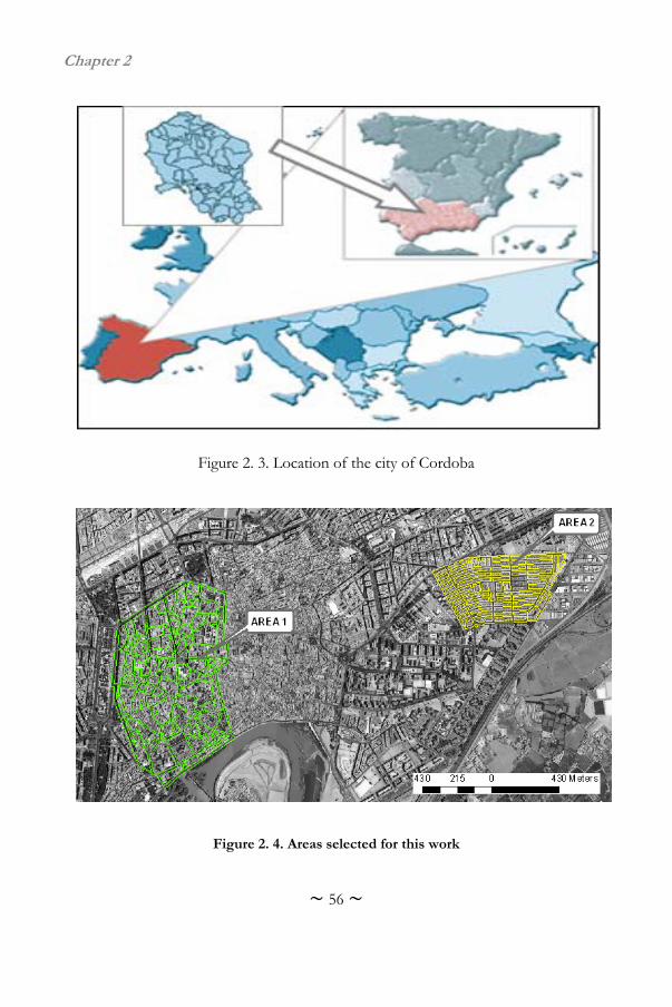
Chapter 2

~ 56 ~ 

 

Figure 2. 3. Location of the city of Cordoba

Figure 2. 4. Areas selected for this work

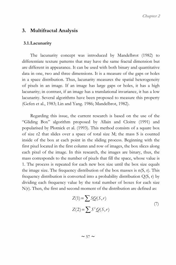
Chapter 2

~ 57 ~ 

 

3. Multifractal Analysis

3.1. Lacunarity

The lacunarity concept was introduced by Mandelbrot (1982) to differentiate texture patterns that may have the same fractal dimension but are different in appearance. It can be used with both binary and quantitative data in one, two and three dimensions. It is a measure of the gaps or holes in a space distribution. Thus, lacunarity measures the spatial heterogeneity of pixels in an image. If an image has large gaps or holes, it has a high lacunarity; in contrast, if an image has a translational invariance, it has a low lacunarity. Several algorithms have been proposed to measure this property (Gefen et al., 1983; Lin and Yang. 1986; Mandelbrot, 1982).

Regarding this issue, the current research is based on the use of the

“Gliding Box” algorithm proposed by Allain and Cloitre (1991) and popularised by Plotnick et al. (1993). This method consists of a square box of size r2 that slides over a space of total size M; the mass S is counted inside of the box at each point in the sliding process. Beginning with the first pixel located in the first column and row of images, the box slices along each pixel of the image. In this research, the images are binary, thus, the mass corresponds to the number of pixels that fill the space, whose value is 1. The process is repeated for each new box size until the box size equals the image size. The frequency distribution of the box masses is n(S, r). This frequency distribution is converted into a probability distribution Q(S, r) by dividing each frequency value by the total number of boxes for each size N(r). Then, the first and second moment of the distribution are defined as:

2

(1) ( , )

(2) ( , )

Z SQ S r

Z S Q S r (7)

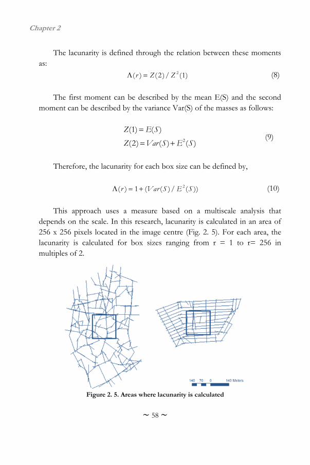
Chapter 2

~ 58 ~ 

 

The lacunarity is defined through the relation between these moments as:

2( ) ( 2 )/ (1)r Z Z (8)

The first moment can be described by the mean E(S) and the second

moment can be described by the variance Var(S) of the masses as follows:

2

(1) ( )

(2) ( ) ( )

Z E S

Z Var S E S (9)

Therefore, the lacunarity for each box size can be defined by,

2( ) 1 ( ( )/ ( ))r Var S E S (10)

This approach uses a measure based on a multiscale analysis that

depends on the scale. In this research, lacunarity is calculated in an area of 256 x 256 pixels located in the image centre (Fig. 2. 5). For each area, the lacunarity is calculated for box sizes ranging from r = 1 to r= 256 in multiples of 2.

Figure 2. 5. Areas where lacunarity is calculated

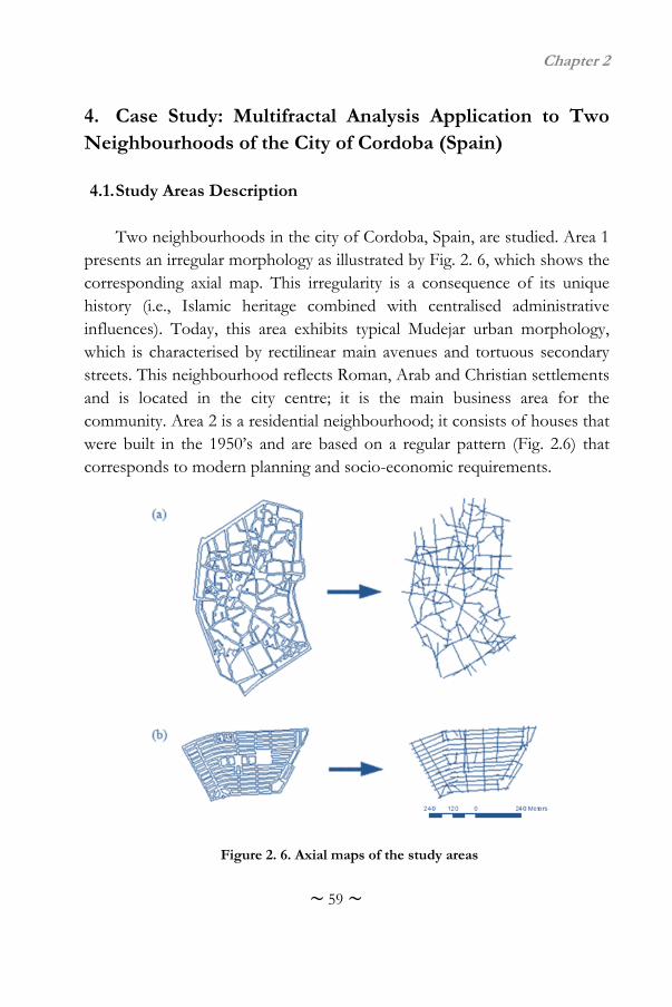
Chapter 2

~ 59 ~ 

 

4. Case Study: Multifractal Analysis Application to Two Neighbourhoods of the City of Cordoba (Spain)

4.1. Study Areas Description

Two neighbourhoods in the city of Cordoba, Spain, are studied. Area 1

presents an irregular morphology as illustrated by Fig. 2. 6, which shows the corresponding axial map. This irregularity is a consequence of its unique history (i.e., Islamic heritage combined with centralised administrative influences). Today, this area exhibits typical Mudejar urban morphology, which is characterised by rectilinear main avenues and tortuous secondary streets. This neighbourhood reflects Roman, Arab and Christian settlements and is located in the city centre; it is the main business area for the community. Area 2 is a residential neighbourhood; it consists of houses that were built in the 1950’s and are based on a regular pattern (Fig. 2.6) that corresponds to modern planning and socio-economic requirements.

Figure 2. 6. Axial maps of the study areas

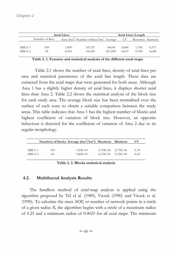
Chapter 2

~ 60 ~ 

 

Area (km2) Average CV Skewness Kurtosis

AREA 1 1,009 146,06 0,604 1,766 0,371AREA 2 0,343 267,849 0,615 0,768 0,628

Axial Lines Length Axial Lines

56167,55

Number of lines Number of lines/km2

169163,40

Table 2. 1. Features and statistical analysis of the different axial maps 

 Table 2.1 shows the number of axial lines, density of axial lines per

area and statistical parameters of the axial line length. These data are extracted from the axial maps that were generated for both areas. Although Area 1 has a slightly higher density of axial lines, it displays shorter axial lines than Area 2. Table 2.2 shows the statistical analysis of the block size for each study area. The average block size has been normalised over the surface of each zone to obtain a suitable comparison between the study areas. This table indicates that Area 1 has the highest number of blocks and highest coefficient of variation of block size. However, an opposite behaviour is detected for the coefficient of variation of Area 2 due to its regular morphology.

Numbers of blocks Average (km2/km2) Maximun Minimun CV

AREA 1 105 7,20E-03 2,70E-02 2,75E-04 0,78AREA 2 69 7,80E-03 6,33E-03 9,55E-04 0,42

 Table 2. 2. Blocks statistical analysis

4.2. Multifractal Analysis Results

The Sandbox method of axial-map analysis is applied using the

algorithm proposed by Tél el al. (1989), Vicsek (1990) and Vicsek et al. (1990). To calculate the mass M(R) or number of network points in a circle of a given radius R, the algorithm begins with a circle of a maximum radius of 0.25 and a minimum radius of 0.0025 for all axial maps. The minimum

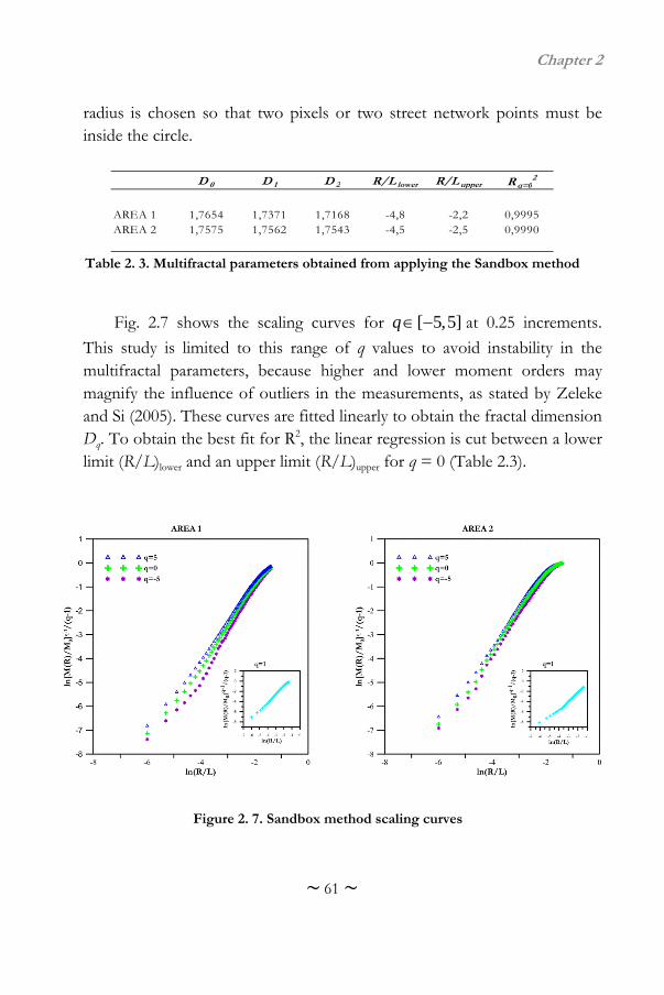
Chapter 2

~ 61 ~ 

 

radius is chosen so that two pixels or two street network points must be inside the circle.

D 0 D 1 D 2 R/L lower R/L upper R q=0

2

AREA 1 1,7654 1,7371 1,7168 -4,8 -2,2 0,9995AREA 2 1,7575 1,7562 1,7543 -4,5 -2,5 0,9990

 Table 2. 3. Multifractal parameters obtained from applying the Sandbox method

Fig. 2.7 shows the scaling curves for [ 5,5]q at 0.25 increments.

This study is limited to this range of q values to avoid instability in the multifractal parameters, because higher and lower moment orders may magnify the influence of outliers in the measurements, as stated by Zeleke and Si (2005). These curves are fitted linearly to obtain the fractal dimension Dq. To obtain the best fit for R2, the linear regression is cut between a lower limit (R/L)lower and an upper limit (R/L)upper for q = 0 (Table 2.3).

Figure 2. 7. Sandbox method scaling curves

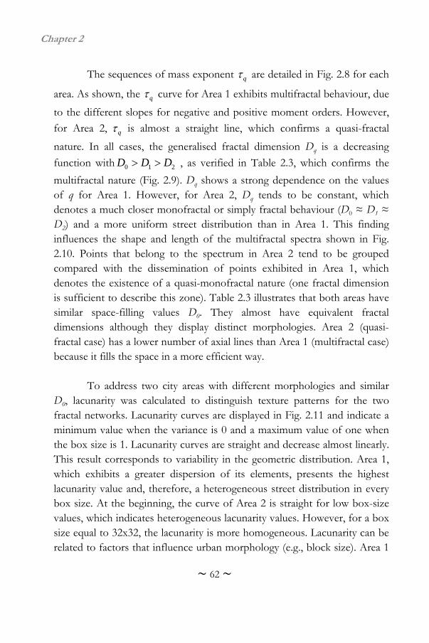
Chapter 2

~ 62 ~ 

 

The sequences of mass exponent q are detailed in Fig. 2.8 for each

area. As shown, the q curve for Area 1 exhibits multifractal behaviour, due

to the different slopes for negative and positive moment orders. However,

for Area 2, q is almost a straight line, which confirms a quasi-fractal

nature. In all cases, the generalised fractal dimension Dq is a decreasing

function with 0 1 2D D D , as verified in Table 2.3, which confirms the

multifractal nature (Fig. 2.9). Dq shows a strong dependence on the values of q for Area 1. However, for Area 2, Dq tends to be constant, which denotes a much closer monofractal or simply fractal behaviour (D0 ≈ D1 ≈ D2) and a more uniform street distribution than in Area 1. This finding influences the shape and length of the multifractal spectra shown in Fig. 2.10. Points that belong to the spectrum in Area 2 tend to be grouped compared with the dissemination of points exhibited in Area 1, which denotes the existence of a quasi-monofractal nature (one fractal dimension is sufficient to describe this zone). Table 2.3 illustrates that both areas have similar space-filling values D0. They almost have equivalent fractal dimensions although they display distinct morphologies. Area 2 (quasi-fractal case) has a lower number of axial lines than Area 1 (multifractal case) because it fills the space in a more efficient way.

To address two city areas with different morphologies and similar

D0, lacunarity was calculated to distinguish texture patterns for the two fractal networks. Lacunarity curves are displayed in Fig. 2.11 and indicate a minimum value when the variance is 0 and a maximum value of one when the box size is 1. Lacunarity curves are straight and decrease almost linearly. This result corresponds to variability in the geometric distribution. Area 1, which exhibits a greater dispersion of its elements, presents the highest lacunarity value and, therefore, a heterogeneous street distribution in every box size. At the beginning, the curve of Area 2 is straight for low box-size values, which indicates heterogeneous lacunarity values. However, for a box size equal to 32x32, the lacunarity is more homogeneous. Lacunarity can be related to factors that influence urban morphology (e.g., block size). Area 1

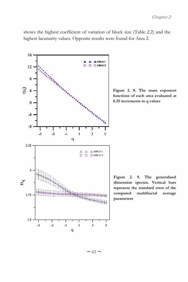
Chapter 2

~ 63 ~ 

 

shows the highest coefficient of variation of block size (Table 2.2) and the highest lacunarity values. Opposite results were found for Area 2.

Figure 2. 8. The mass exponentfunctions of each area evaluated at0.25 increments in q values

Figure 2. 9. The generaliseddimension spectra. Vertical barsrepresent the standard error of thecomputed multifractal averageparameters

 

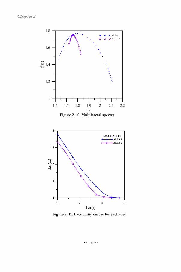
Chapter 2

~ 64 ~ 

 

Figure 2. 10. Multifractal spectra

Figure 2. 11. Lacunarity curves for each area

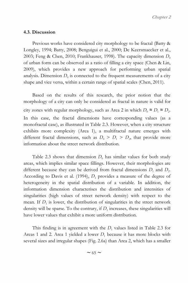
Chapter 2

~ 65 ~ 

 

4.3. Discussion

Previous works have considered city morphology to be fractal (Batty & Longley, 1994; Batty, 2008; Benguigui et al., 2000; De Keersmaecker et al., 2003; Feng & Chen, 2010; Frankhauser, 1998). The capacity dimension D0 of urban form can be observed as a ratio of filling a city space (Chen & Lin, 2009), which provides a new approach for performing urban spatial analysis. Dimension D0 is connected to the frequent measurements of a city shape and vice versa, within a certain range of spatial scales (Chen, 2011).

Based on the results of this research, the prior notion that the

morphology of a city can only be considered as fractal in nature is valid for

city zones with regular morphology, such as Area 2 in which D0 ≈ D1 ≈ D2.

In this case, the fractal dimensions have corresponding values (as a monofractal case), as illustrated in Table 2.3. However, when a city structure exhibits more complexity (Area 1), a multifractal nature emerges with different fractal dimensions, such as D0 > D1 > D2, that provide more information about the street network distribution.

Table 2.3 shows that dimension D0 has similar values for both study

areas, which implies similar space fillings. However, their morphologies are different because they can be derived from fractal dimensions D1 and D2. According to Davis et al. (1994), D1 provides a measure of the degree of heterogeneity in the spatial distribution of a variable. In addition, the information dimension characterises the distribution and intensities of singularities (high values of street network density) with respect to the mean. If D1 is lower, the distribution of singularities in the street network density will be sparse. To the contrary, if D1 increases, these singularities will have lower values that exhibit a more uniform distribution.

This finding is in agreement with the D1 values listed in Table 2.3 for

Areas 1 and 2. Area 1 yielded a lower D1 because it has more blocks with several sizes and irregular shapes (Fig. 2.6a) than Area 2, which has a smaller

Chapter 2

~ 66 ~ 

 

number of blocks that are similar in size and resemble rectangles (Fig. 2.6b). This finding is consistent with the CV values shown in Table 2 (CVArea 1 > CVArea 2). When D0 = D1, a monofractal case exists. This description might be valid for Area 2; however, it is not valid for Area 1 (D0 > D1), which exhibits a multifractal nature.

Correlation dimension D2 describes the uniformity of the street

network density among several selected zones (circles of radius R). D2 is related to the probability of finding pixels that belong to the street network within a given distance when beginning on a pixel that belongs to this object. D2 is confirmed to be higher for Area 2 (Table 2.3) and more uniform than Area 1, as shown by Fig. 2.6. As in the case of D1, this finding is a result of relevant differences in the number, size and shape of blocks that determine the analysed morphologies of the neighbourhood. Area 2 can be considered quasi-fractal because D0 ≈ D2, whereas Area 1 has a multifractal nature (D0 > D2), as previously stated.

According to these results, the Rényi dimension spectrum can be used

to describe urban morphology instead of a single-valued fractal dimension. This situation is determined by different urban morphology generative processes (city growth according to several planning/socio-economic regulations) over time, which results in regular and irregular areas.

Chapter 2

~ 67 ~ 

 

5. Conclusions

With the goal of performing a multifractal analysis of urban morphology, street layouts are extracted using a Space Syntax algorithm for two urban neighbourhoods, thereby obtaining axial maps of each area to accurately represent their spatial configurations. The Sandbox multifractal method and lacunarity measurements are applied to describe street networks. Multifractal analysis is efficient for characterising the morphology of street networks with the advantage of parameters that are independent over a range of scales. According to the generalised dimension spectra obtained in this research, it is convenient to consider the existence of the multifractal nature of some urban zones, especially when addressing cities with frequent irregular morphology; these areas cannot be described by a single fractal dimension as previous research states. Instead, infinite fractal dimensions for these zones should be theoretically considered. In practice, capacity, information and correlation fractal dimensions are sufficient parameters for characterising irregular morphologies.

This research is based on a case study of two neighbourhoods in the

same city. Although the regular and irregular urban patterns studied here are frequently observed in other cities, the replication of this analysis would establish the generality of the conclusions reached in the case study of Cordoba.

The differences found for the fractal dimensions obtained for the

neighbourhoods in this research are influenced by urban patterns derived from planning regulations and diverse socio-economic situations, such as the spatial and temporal evolution of land values (i.e., Hu et al., 2012). Thus, with the objective of aiding urban planning and management, further analyses should be performed to relate specific fractal dimensions to different planning and socio-economic regimes. The study of relationships between fractal dimensions and market context is suggested because the city street network is determined by business principles in many cases.

Chapter 2

~ 68 ~ 

 

List of References

Allain, C., & Cloitre, C. (1991). Characterizing the lacunarity of random and deterministic fractal sets. Phys. Rev. A, 44, 3552 – 3558.

Allen, J., & Lu, K. (2003). Modeling and prediction of future urban growth

in the Charleston region of South Carolina: a GIS-based integrated approach. Conserv. Ecol., 8(2), 2.

Alves Junior, S., & Barros Filho, M. (2005). Enhancing urban analysis

through lacunarity multiscale measurement. London: University College London.

Amorim, L., Barros Filho, M.N., & Cruz, D. (2009). Urban Texture and

Space Configuration. Proceedings of the 7th International Space Syntax Symposium, Stockholm.

Batty, M., & Longley, P. A. (1987). Urban shapes as fractals. Area, 19(3),

215 – 221. Batty, M., & Longley, P. A. (1994). Fractal Cities: A Geometry of Form and

Function. (3rd ed.) London: Academic Press. Batty, M. (2008). The size, scale, and shape of cities. Science, 319, 769 –

771. Benguigui, L., Czamanski, D., Marinov, M., & Portugali, J. (2000). When

and where is a city fractal? Environ. Plan. B: Plan. Des., 27, 507 – 519. Chen, Y. (2009). Analogies between urban hierarchies and river networks:

fractals, symmetry, and self-organized criticality. Chaos Soliton. Fract., 40(4), 1766 – 1778.

Chapter 2

~ 69 ~ 

 

Chen, Y., & Lin, J. (2009). Modeling the self-affine structure and optimization conditions of city systems using the idea from fractals. Chaos Soliton. Fract., 41, 615 – 629.

Chen, Y. (2011). Derivation of the functional relations between fractal

dimension of and shape indices of urban form. Comput. Environ. Urban, 35, 442 – 451.

Croxford, B., Penn, A., & Hillier, B. (1996). Spatial distribution of urban

pollution: civilizing urban traffic. Sci. Total Environ., 189 – 190, 3 – 9. Czerkauer-Yamu, C., & Frankhauser, P. (2010). A multi-scale (multi-fractal)

approach for a systemic planning strategy from a regional to an architectural scale. REAL CORP 2010 Proceedings/Tagungsband, Vienna (Austria).

Davis, A., Marshak, A., Wiscombe, W., &, Cahalan, R. (1994). Multifractal

characterization of non stationarity and intermitency in geophysical fields: observed, retrieved or simulated. J. Geophys. Res., 99, 8055 – 8072.

De Bartolo, S. G., Grabiele, S., & Gaudio, R. (2000). Multifractal behaviour

river networks. Hydrol. Earth. Syst. SC, 4(1), 105 – 112. De Bartolo, S.G., Gaudio, L., & Gabriele, S. (2004). Multifractal analysis of

river network: sandbox approach. Water Resour. Res., 40(2), W02201, doi: 10.1029/2003WR002760.

De Bartolo, S.G., Veltri, M., & Primavera, L. (2006). Estimated generalized

dimensions of river networks. J. Hydrol., 322 (1 – 4), 181 – 191. De Keersmaecker, M.L., Frankhauser, P., & Thomas, I. (2003). Using

fractal dimensions for characterizing intra-urban diversity: the example of Brussels. Geogr. Anal., 35, 310 – 328.

Chapter 2

~ 70 ~ 

 

Dickinson, R. E. (1961). The West European City. A Geographical Interpretation (2nd ed.). London: Routledge and Kegan Paul Ltd.

Duan, Z.Y., & Wang Q. (2009). Road network analysis and evaluation of

Huizhou city based on space syntax. 2009 International Conference on Measuring Technology and Mechatronics Automation. Compcon. IEEE., 3, 579 – 582.

DTLR & CABE (2001). By Design: Better Places to Live. A companion

guide to PPG3. Tonbridge: Thomas Telford. Encarnação, S., Gaudiano, M., Santos, F.C., Tenedório, J.A., & Pacheco,

J.M. (2012). Fractal cartography of urban areas. Sci. Rep., 2, Article Number: 527.

Escobar-Camacho, J. M. (1997). La Ciudad de Córdoba Tras la

Reconquista. Córdoba en la Historia: la Construcción de la Urbe (Cordoba after the Reconquest. Cordoba into History: the Building of a City). (1st ed.). Barcelona: Caixa Fundacion.

Escobar-Camacho, J.M. (1987). El Recinto Amurallado de la Ciudad de

Córdoba Bajomediaval. La Ciudad Hispánica Siglos XII al XVI (Cordoba Walls in the Early Middle Ages. The Hispanic City in Centuries XII-XVI). (1st ed.) .Madrid: Universidad Complutense.

Escolano Utrilla, S. (2007). La medida de la segregación residencial urbana:

análisis multiescala mediante índices de lagunaridad (The measurement of the urban residential segregation: multi-scale analysis using lacunarity indices). GeoFocus, 7, 216 – 234.

Falconer, K. J. (1990). Fractal Geometry: Mathematical Foundations and

Applications. (2nd ed.). Chichester: John Wiley.

Chapter 2

~ 71 ~ 

 

Frankhauser, P. (1998). The fractal approach: a new tool for the spatial analysis of urban agglomerations. population: An English Selection, 10: 205 – 240.

Feng, J., & Chen, Y. (2010). Spatiotemporal evolution of urban form and

land use structure in Hangzhou, China: evidence from fractals. Environ. Plan. B: Plan. Des., 37, 838 – 856.

Folorunso, O. A., Puente, C. E., Rolston, D. E., & Pinzon, J. E. (1994).

Statistical and fractal evaluation of the spatial characteristics of soil surface strength. Soil. Sci. Soc. Am. J., 58, 284 – 294.

García-Verdugo, F.R. (1997). La formación de la ciudad contemporánea. El

desarrollo urbanístico cordobés en los siglos XIX Y XX. Córdoba en la Historia: la Construcción de la Urbe (Contemporary City Building. Cordoba Urban Development in Centuries XIX and XX. Cordoba into History: the Building of a City). (1st ed.). Barcelona: Caixa Fundacion.

Gefen, Y., Meir, Y., & Aharony, A. (1983). Geometric implementations of

hipercubic lattices with noninteger dimensionality by use of low lacunarity lattices. Phys. Rev. Lett., 50, 145 – 148.

Hillier B., & Hanson, J. (1984). The Social Logic of Space. (7th ed.).

Cambridge: Cambridge University Press. Hu, M.B., Jiang, R., Wang, R., & Wu, Q.S. (2009). Urban traffic simulated

from the dual representation: flow, crisis and congestion. Phys. Lett. A., 373(23–24), 2007 – 2011.

Hu, S., Cheng, Q., & Wang, L. (2012). Multifractal characterization of urban

residential land price in space and time. App. Geogr., 34, 161–170.

Chapter 2

~ 72 ~ 

 

Jeong, S.K., & Ban, Y.U. (2011). Computational algorithms to evaluate design solutions using Space Syntax. Comput.-Aided Des., 43, 664 – 676.

Jiang, B. (2007). Ranking spaces for predicting human movement in an urban environment. Int. J. Geogr. Inf. Sci. 23(7), 823 – 837.

Jiang, B., & Claramunt, C. (2002). Integration of space into GIS: new

perspectives for urban morphology. Trans. in GIS, 6(3), 295 – 309. Jiang, B., Claramunt, C., & Batty, M. (1999). Geometric accessibility and

geographic information: extending desktop GIS to space syntax. Comput. Environ. Urban. 23, 127 – 146.

Jiang, B., & Liu, X. (2009a). AxialGen: a research prototype for

automatically generating the axial lines. Proceedings of CUPUM 2009, the 11th International Conference on Computers in Urban Planning and Urban Management, Hong Kong.

Kravchenko, A.N., Boast, C.W., & Bullock, D.G. (1999). Multifractal

analysis of soil spatial variability. Agron. J., 91(6), 1033–1041. Lee, C. K. (2002). Multifractal characteristics in air pollutant concentration

time series. Water Air Soil. Poll., 135, 389 – 409. Lin, B., & Yang, Z.R. (1986). A suggested lacunarity expression for

Sierpinski carpets. J. Phys. A: Math. Gen., 19, L49 – L52. Lynch, K. (1981). A Theory of Good City Form. Cambridge: MIT Press. Mach, J., Mas, F., & Sagues F. (1995). Two representations in multifractal

analysis. J Phys. A-Math. Gen., 28, 5607 – 5622. Major, M.D., Penn, A., & Hillier, B. (1997). The Question does compute

the role of the computer in the space syntax. Compt. Environ. Urban. 3, 42.1 – 42.7.

Chapter 2

~ 73 ~ 

 

Mandelbrot, B.B. (1982). The fractal geometry of nature. New York: W.H.

Freeman and Company. Marshall, S. (2005). Streets Patterns. London and New York: Spon Press. Milne, B.T. (1990). Lessons from applying fractals models to landscape

patterns. In Turner, M.G., & Gardner, R.H., (Eds.), Quantitive methods in landscape ecology (pp. 200–235). New York: Springer-Verlag.

Myint, S.W., & Lam, N. (2005). A study of lacunarity-based texture analysis

approaches to improve urban image classification. Comput. Environ. Urban. Syst. 29, 501 – 523.

Penn, A., Conroy, R., Dalton, N., Dekker, L., Mottram, C., & Turner, A.

(1997). Intelligent architecture: new tools for the three dimensional analysis of space and built form. First International Symposium on Space Syntax. University College London, U.K. 2, 30.1 – 30.19.

Peponis, J., Wineman, J., Bafna, S., Rashid, M., & Kim, S.H. (1998). On the

generation of linear representations of spatial configuration. Environ. Plann. B., 25, 559 – 576.

Plotnick, R. E., Gardner, R. H., Hargrove, W. W., Prestegaard, K., &

Perlmutter, M. (1996). Lacunarity analysis: a general technique for the analysis of spatial patterns. Phys. Rev. E., 53, 5461 – 5468.

Plotonick, R.E., Gardner, R.H., & O´Neill, R.V. (1993). Lacunarity indices

as measures of landscape texture. Landsc. Ecol., 8 (3), 201 – 211. Rinaldo, A., Rodriguez-Iturbe, I., Rigon, R., Ijjasz-Vasquez, E., & Bras, R.L.

(1993). Self-organized fractal river networks. Phys. Rev. Lett., 70(6), 822 – 825.

Chapter 2

~ 74 ~ 

 

Stanley, H. E., & Meakin, P. (1988). Multifractal phenomena in physics and chemistry. Nature., 335, 405 – 409.

Tél, T., Fülöp, Á., & Vicsek, T. (1989). Determination of fractal dimensions

for geometrical multifractals. Phys. A., 159, 155 – 166. Thomas, I., Frankhauser, P.,& Badariotti, D. (2012). Comparing the

fractality of European urban neighborhoods: do national contexts matter? J. Geogr. Syst., 14(2), 189 – 208.

Turner, A. (2006). The ingredients of an Exosomatic Cognitive Map.

Isovist, Agents and Axial Lines?. Space Syntax and Spatial Cognition Proceedings, Bremen.

Turner, A., Penn, A., & Hillier, B. (2005). An algorithmic definition of the

axial map. Environ. Plann. B., 25, 425 – 444. Van Diepen, A., & Henk, V. (2003). Sustainability and planning: does urban

form matter?. Int. J. Sust. Dev. World., 4, 59 – 74. Vaquerizo-Gil, D. (2003). Guía Arqueológica de Córdoba (Archaeological

Guide of Cordoba). (1st ed.). Cordoba: Plurabelle. Vicsek, T. (1990). Mass multifractal. Phys. A., 168, 490 – 497. Vicsek, T., Family, F., & Meakin, P. (1990). Multifractal geometry of

diffusion- limited aggregates. Europhys., 12(3), 217 – 222. Wu, X. B., & Sui, D. Z. (2001). An initial exploration of a lacunarity-based

segregation measure. Environ. Plann. B., 28(3), 433 – 446. Xiao, J., Shen, Y., Ge, J., Tateishi, R., Tang, C., Liang, Y., & Huang, Z.

(2006). Evaluating urban expansion and land use change in

Chapter 2

~ 75 ~ 

 

Shijiazhuang, China, by using GIS and remote sensing. Landscape Urban Plan., 75, 69 – 80.

Zeleke, T.B., & Si, B.C. (2005). Scaling relationships between saturated

hydraulic conductivity and soil physical properties. Soil Sci. Soc. Am. J., 69 (6), 1691 – 1702.

Chapter 2

~ 76 ~ 

 

 

~ 77 ~ 

 

Chapter 3  

 

“Un gran árbol transpira cada día cientos de litros de agua a la atmósfera. No hay troncos

ni ramas en el bosque, sino canales disfrazados por donde corre el agua. Troncos líquidos, copas verdes, el sol

arriba… ¿Cómo? ¿Qué no es un árbol? ¿Y las flores? ¿Caballos, dice?

¿Es una ensoñación? ¿Será fractal la materia de los sueños de Shakespeare?”

Miguel Delibes de Castro (1947- )

 

~ 78 ~ 

 

  

Chapter 3

~ 79 ~ 

 

Chapter 3. Multifractal

analysis applied to the study of the accuracy of DEM-based stream derivation.

Abstract  

A correct description of river network morphology is very important when it is used to study different features of a river’s morphology as well as phenomena related to it such as erosion, nitrogen retention or sediment pollution. Different algorithms have been developed to extract drainage networks directly from Digital Elevation Models. In this paper, the suitability of ArcHydro extension, developed for ArcGIS Desktop and based on the D8 algorithm for generating river networks, has been studied by using multifractal analysis. This approach allows the determination of a suitable flow accumulation threshold value by considering the Rényi spectra. The river networks generated by ArcHydro were compared to those provided by photogrammetric restitution by taking into account the multifractal spectra showing differences in stream density with a low channel order. In this work, the use of multifractal analysis has been extended as a pattern recognition tool for completing human perception when images are visually checked.  

 

KEYWORDS: river networks; multifractal analysis; digital elevation model; pattern recognition; flow accumulation threshold value.  

Chapter 3

~ 80 ~ 

 

1. Introduction It is of great importance to know about a river’s morphology

because this can be used to study its relationship to nitrogen retention (Alexander et al. 2000, Wagenschein & Rode 2007), erosion (Vital et al., 1998, Prosser et al. 2001, Makaske et al. 2009) or rainfall (Ramos and Gracia 2011), among other phenomena. Geographic Information Systems (GIS) are suitable tools for researching different river features, as well as their corresponding watersheds. Thus, GISs have been applied to find out the risk of erosion in catchments (Winterbottom et al. 2000, Nigel et al., 2010), river contamination by sediments (Terrado et al. 2006, Rhoades et al. 2008, Siber et al. 2009, Delgado et al. 2010) and the change in channel morphology of rivers (Porter & Massong 2004). River networks can be obtained directly by digitization from the interpretation of digital images or through a Digital Elevation Model (DEM) by using GIS tools. Different algorithms have been developed to extract basic topographic characteristics from DEMs related to hydrology, such as those calculated for river networks (Mark 1984, O’ Callaghan & Mark 1984) and catchment boundaries (Morris & Heerdegen 1988). The first approach to extracting river networks from a DEM was D8 algorithm, introduced by O’Callaghan and Mark (1984), using a neighbourhood of eight cells as possible flow directions. This algorithm is probably the most popular method for automated drainage recognition and catchment area determinations (Martz & Garbrecht, 1998). However, results of applying this method are sometimes non-realistic (Turcotte et al., 2001), due to the determination of the flow in only one of eight possible directions, the presence of flat areas and pits, and the lack of information on the locations of lakes. The multiple flow direction method, in which the drainage of a particular cell flows down slope to several adjacent cells of a lower elevation, was suggested (Freeman, 1991) to overcome the limitations of D8. This approach does improve the D8 model in some aspects, but needs additional computational time to calculate a greater density of flow connections (Gallant & Wilson, 1996), and the flow from a pixel is dispersed to all the neighbouring pixels with lower elevation. Lea (1992) developed an algorithm that calculates the flow

Chapter 3

~ 81 ~ 

 

direction through the aspect associated with each cell. The flow is routed as though it were a ball rolling on a plane released from the centre of each cell. A plane is fitted to the elevations of pixel corners, these corner elevations being estimated by averaging the elevations of adjoining pixel centre elevations. This algorithm has the advantage of specifying flow direction continuously and without dispersion. Costa-Cabral and Burges (1994) developed the DEMON (Digital Elevation Model Network) algorithm to try to improve the modelling proposed by Lea (1992). Grid elevation values are used as pixel corners, rather than block centred, and a plane surface is fitted for each pixel. They recognized flow as being two-dimensional, originating uniformly over the pixel area, rather than tracking flow paths from the centre point of each pixel. The plane flow methods (Lea, 1992; Costa-Cabral & Burges, 1994) are deterministic and resolve flow directions. However, they are susceptible to problems arising from the approximation involved in fitting a plane through four points (Tarboton, 1997). Tarboton (1997) used multiple flow directions to resolve the limitations of the D8 algorithm, but the main problem of this method is the elimination of the unimodal link between the flow directions and the difficulty in calculating the catchment boundary due to the multiple flow direction from a cell.

 

Several authors have developed software tools including some of these algorithms to calculate river networks from a DEM. Among others, these tools are: i) ArcHydro , an extension for the ArcGIS Desktop developed by the University of Texas (Maidment 2002) based on the maximum gradient method, D8 algorithm, proposed by O´ Callaghan et al. in 1984; ii) CUENCAS which extracts the drainage structure from a DEM using algorithms which is centred on a D8 algorithm (Mantilla & Gupta 2005); iii) GRASS which is a toolset designed for the Hortonian analysis of drainage networks and uses a multiple flow direction algorithm for stream network extraction (Jasiewicz & Mezt 2011). Despite the drawbacks of the D8 algorithm explained before, it is used in this work to extract the drainage network from a DEM, because it is frequently applied in hydrological research. However, the suitable determination of the flow accumulation threshold value is a key point that remains open in this algorithm. In this

Chapter 3

~ 82 ~ 

 

sense, it is appropriate to explore this issue by using approaches such as the multifractal analysis that has been applied to studying the morphology of river networks with successful results (Rinaldo et al. 1993, De Bartolo et al. 2000, 2004, 2006). The multifractal analysis based on the Box-counting fixed-size methods has one main dedefct, i.e. an incorrect determination of the fractal dimensions for negative moment orders, due to the emphasis given to regions with few points not centred on them (e.g., De Bartolo et al., 2004, Gaudio et al., 2006). Some errors, due to the use of Legendre transforms (Veneziano et al., 1995), are associated with such problems, leading to a poor estimation of the multifractal spectrum (De Bartolo et al., 2006).This snag can be minimized by using the Sandbox algorithm (Tél et al., 1989; Vicsek, 1990; Vicsek et al., 1990), that is also a fixed-size method. According to De Bartolo et al. (2004), the disadvantage of the presence of regions containing few data points has been overcome, and, therefore, the principal cause of the biased assessment of the generalized fractal dimensions for negative moment orders has been removed. This circumstance could be especially interesting when describing the morphology of river networks, where regions with a small number of streams are frequent. This approach has been applied to the study of the morphology of river networks to analyze different variables such as the influence of lithological and tectonic morphologies on river (Gaudio et al. 2005, Dombrádi et al. 2007).

 

This work explores the use of the Sandbox algorithm in the study of quality river network morphology generated by the extension ArcHydro tool, which applies the D8 algorithm, correcting the presence of pits and offering the possibility of including information on the locations of lakes. The rivers have been generated from a DEM and they have been compared to a river network proceeding from photogrammetric restitution provided by the Department of Agriculture, Fisheries and Environment, Government of Andalusia, 2005. The DEM, which has a 10 meters resolution, was provided by the Department for Public Works and Transport (Government of Andalusia). It was obtained in 2005 from aerial photographs (scale 1: 20.000). The study area (Fig.3. 1) corresponds to

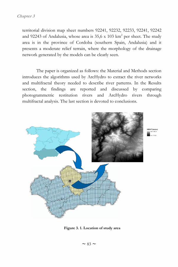
Chapter 3

~ 83 ~ 

 

territorial division map sheet numbers 92241, 92232, 92233, 92241, 92242 and 92243 of Andalusia, whose area is 35,6 x 103 km2 per sheet. The study area is in the province of Cordoba (southern Spain, Andalusia) and it presents a moderate relief terrain, where the morphology of the drainage network generated by the models can be clearly seen.

 

The paper is organized as follows: the Material and Methods section introduces the algorithms used by ArcHydro to extract the river networks and multifractal theory needed to describe river patterns. In the Results section, the findings are reported and discussed by comparing photogrammetric restitution rivers and ArcHydro rivers through multifractal analysis. The last section is devoted to conclusions.

Figure 3. 1. Location of study area

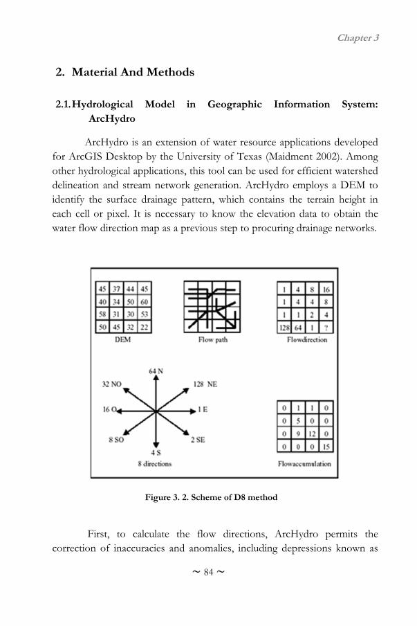
Chapter 3

~ 84 ~ 

 

2. Material And Methods

2.1. Hydrological Model in Geographic Information System: ArcHydro

ArcHydro is an extension of water resource applications developed for ArcGIS Desktop by the University of Texas (Maidment 2002). Among other hydrological applications, this tool can be used for efficient watershed delineation and stream network generation. ArcHydro employs a DEM to identify the surface drainage pattern, which contains the terrain height in each cell or pixel. It is necessary to know the elevation data to obtain the water flow direction map as a previous step to procuring drainage networks.

First, to calculate the flow directions, ArcHydro permits the

correction of inaccuracies and anomalies, including depressions known as

Figure 3. 2. Scheme of D8 method

Chapter 3

~ 85 ~ 

 

sinks. These anomalies can prevent the water from flowing along the channels and becoming accumulated. Once these anomalies are corrected, ArcHydro assigns a flow direction to each pixel, which depends on the maximum slope of the cells around it. As shown in Fig. 3. 2, extracted from ArcHydro Tutorial, there are eight flow directions. Once the flow direction map is known, a flow accumulation map is calculated and the number of cells that pour into a given cell is attributed to each pixel. Finally, the river maps are defined with the length of each stream depending on the threshold value considered for flow accumulations. The default value displayed by ArcHydro for the river threshold represents 1% of the maximum flow accumulation, but any other threshold value can be selected (Maidment 2002).

 

 

3. Results This study explores the suitability of river networks simulated by

ArcHydro from a DEM of 10 m in cell size. The multifractal Sandbox method was used to determine the Rényi spectra of the networks provided by ArcHydro and those calculated from photogrammetric restitution. By comparing these spectra, it was possible to yield the suitable flow accumulation threshold value for obtaining the most accurate ArcHydro results, as well as determining the resemblance between both kinds of networks. In order to compare both networks correctly, the data provided from photogrammetric restitution were previously processed due to the main rivers being represented by a double line describing their edges. This fact can produce wrong results when the river networks are compared, because river networks generated by ArcHydro are represented by a line. Therefore, the photogrammetric restitution main rivers were described by a central line calculated in ArcGIS.

To apply the multifractal Sandbox method to obtain the Rényi spectra,

the calculation of M(R), or number of network points in a circle of a given

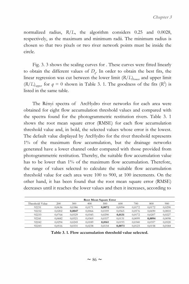
Chapter 3

~ 86 ~ 

 

normalized radius, R/L, the algorithm considers 0.25 and 0.0028, respectively, as the maximum and minimum radii. The minimum radius is chosen so that two pixels or two river network points must be inside the circle.

Fig. 3. 3 shows the scaling curves for . These curves were fitted linearly

to obtain the different values of Dq. In order to obtain the best fits, the linear regression was cut between the lower limit (R/L)lower and upper limit (R/L)upper for q = 0 shown in Table 3. 1. The goodness of the fits (R2) is listed in the same table.

The Rényi spectra of ArcHydro river networks for each area were

obtained for eight flow accumulation threshold values and compared with the spectra found for the photogrammetric restitution rivers. Table 3. 1 shows the root mean square error (RMSE) for each flow accumulation threshold value and, in bold, the selected values whose error is the lowest. The default value displayed by ArcHydro for the river threshold represents 1% of the maximum flow accumulation, but the drainage networks generated have a lower channel order compared with those provided from photogrammetric restitution. Thereby, the suitable flow accumulation value has to be lower than 1% of the maximum flow accumulation. Therefore, the range of values selected to calculate the suitable flow accumulation threshold value for each area were 100 to 900, at 100 increments. On the other hand, it has been found that the root mean square error (RMSE) decreases until it reaches the lower values and then it increases, according to

Threshold Value 200 300 400 500 600 700 800 90092231 0,0636 0,0386 0,0171 0,0072 0,0094 0,0172 0,0172 0,029092232 0,0202 0,0047 0,0066 0,0359 0,0565 0,0576 0,0690 0,081092233 0,0764 0,0529 0,0345 0,0290 0,0131 0,0172 0,0207 0,022792241 0,0682 0,0521 0,0369 0,0337 0,0131 0,0099 0,0094 0,009892242 0,0294 0,0245 0,0189 0,0161 0,0193 0,0340 0,0357 0,052092243 0,0516 0,0331 0,0238 0,0154 0,0073 0,0123 0,0158 0,0184

Root Mean Square Error

Table 3. 1. Flow accumulation threshold value selected.

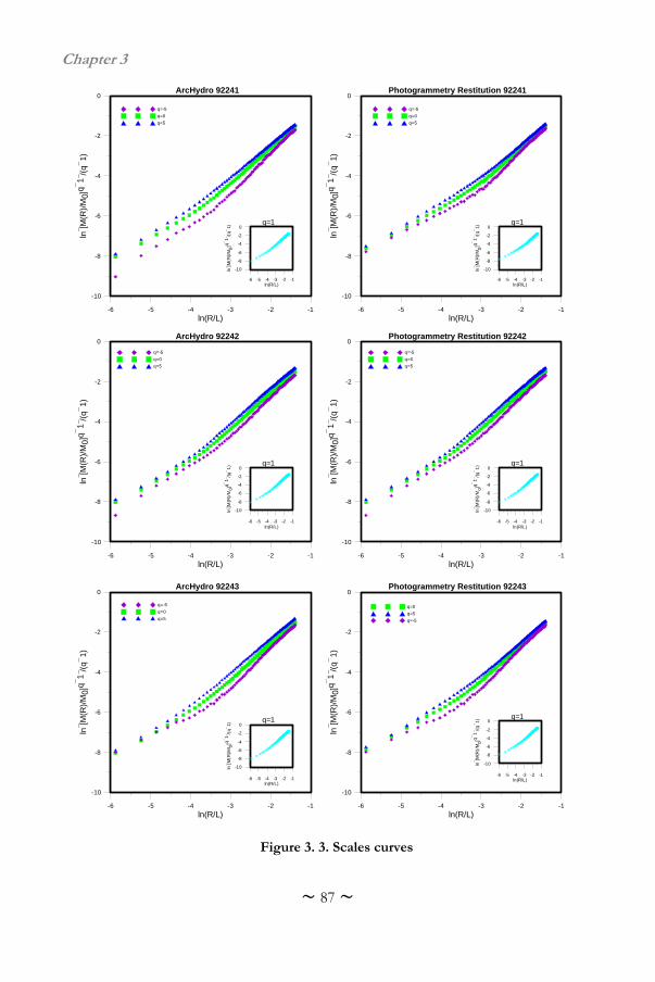
Chapter 3

~ 87 ~ 

 

-6 -5 -4 -3 -2 -1

ln(R/L)

-10

-8

-6

-4

-2

0

ln[M

(R)/

M0]

q1/(

q1)

q=-5

q=0

q=5

ArcHydro 92241

-6 -5 -4 -3 -2 -1ln(R/L)

-10

-8

-6

-4

-2

0ln[M

(R)/

M0

]q1

/(q

1)q=1

-6 -5 -4 -3 -2 -1

ln(R/L)

-10

-8

-6

-4

-2

0

ln[M

(R)/

M0]

q1/(

q1)

q=-5

q=0

q=5

Photogrammetry Restitution 92241

-6 -5 -4 -3 -2 -1ln(R/L)

-10

-8

-6

-4

-2

0

ln[M

(R)/

M0

]q1

/(q

1)

q=1

-6 -5 -4 -3 -2 -1

ln(R/L)

-10

-8

-6

-4

-2

0

ln[M

(R)/

M0

]q1

/(q

1)

q=-5

q=0

q=5

ArcHydro 92242

-6 -5 -4 -3 -2 -1ln(R/L)

-10

-8

-6

-4

-2

0

ln[M

(R)/

M0]

q1

/(q

1) q=1

-6 -5 -4 -3 -2 -1

ln(R/L)

-10

-8

-6

-4

-2

0ln[M

(R)/

M0

]q1

/(q

1)

q=-5

q=0

q=5

Photogrammetry Restitution 92242

-6 -5 -4 -3 -2 -1ln(R/L)

-10

-8

-6

-4

-2

0

ln[M

(R)/

M0]q

1 /(

q1

) q=1

-6 -5 -4 -3 -2 -1

ln(R/L)

-10

-8

-6

-4

-2

0

ln[M

(R)/

M0]

q1/(

q1)

q=0

q=5

q=-5

Photogrammetry Restitution 92243

-6 -5 -4 -3 -2 -1ln(R/L)

-10

-8

-6

-4

-2

0

ln[

M(R

)/M

0]q1

/(q1

) q=1

-6 -5 -4 -3 -2 -1

ln(R/L)

-10

-8

-6

-4

-2

0

ln[M

(R)/

M0]

q1/(

q1)

q=-5

q=0

q=5

ArcHydro 92243

-6 -5 -4 -3 -2 -1ln(R/L)

-10

-8

-6

-4

-2

0

ln[M

(R)/

M0

]q1

/(q

1)

q=1

Figure 3. 3. Scales curves

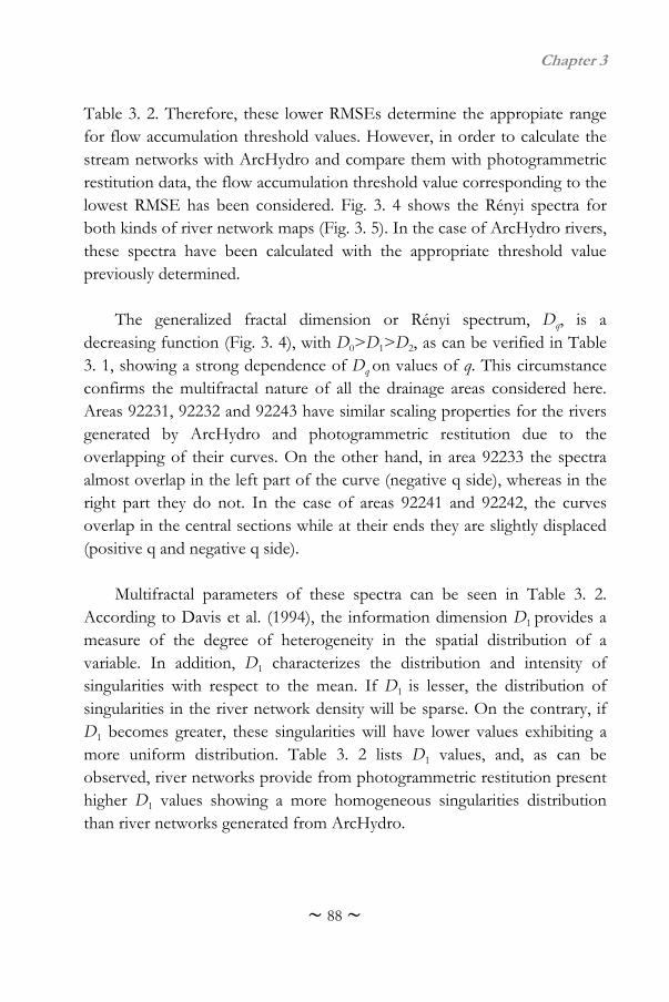
Chapter 3

~ 88 ~ 

 

Table 3. 2. Therefore, these lower RMSEs determine the appropiate range for flow accumulation threshold values. However, in order to calculate the stream networks with ArcHydro and compare them with photogrammetric restitution data, the flow accumulation threshold value corresponding to the lowest RMSE has been considered. Fig. 3. 4 shows the Rényi spectra for both kinds of river network maps (Fig. 3. 5). In the case of ArcHydro rivers, these spectra have been calculated with the appropriate threshold value previously determined.

The generalized fractal dimension or Rényi spectrum, Dq, is a

decreasing function (Fig. 3. 4), with D0>D1>D2, as can be verified in Table 3. 1, showing a strong dependence of Dq on values of q. This circumstance confirms the multifractal nature of all the drainage areas considered here. Areas 92231, 92232 and 92243 have similar scaling properties for the rivers generated by ArcHydro and photogrammetric restitution due to the overlapping of their curves. On the other hand, in area 92233 the spectra almost overlap in the left part of the curve (negative q side), whereas in the right part they do not. In the case of areas 92241 and 92242, the curves overlap in the central sections while at their ends they are slightly displaced (positive q and negative q side).

Multifractal parameters of these spectra can be seen in Table 3. 2.

According to Davis et al. (1994), the information dimension D1 provides a measure of the degree of heterogeneity in the spatial distribution of a variable. In addition, D1 characterizes the distribution and intensity of singularities with respect to the mean. If D1 is lesser, the distribution of singularities in the river network density will be sparse. On the contrary, if D1 becomes greater, these singularities will have lower values exhibiting a more uniform distribution. Table 3. 2 lists D1 values, and, as can be observed, river networks provide from photogrammetric restitution present higher D1 values showing a more homogeneous singularities distribution than river networks generated from ArcHydro.

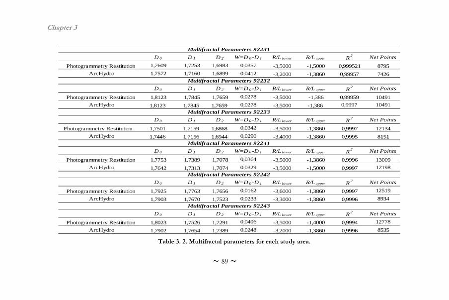
Chapter 3

~ 89 ~ 

 

D 0 D 1 D 2 W=D 0 -D 1 R/L lower R/L upper R2 Net Points

Photogrammetry Restitution 1,7609 1,7253 1,6983 0,0357 -3,5000 -1,5000 0,999521 8795

ArcHydro 1,7572 1,7160 1,6899 0,0412 -3,2000 -1,3860 0,99957 7426

D 0 D 1 D 2 W=D 0 -D 1 R/L lower R/L upper R2 Net Points

Photogrammetry Restitution 1,8123 1,7845 1,7659 0,0278 -3,5000 -1,386 0,99959 10491

ArcHydro 1,8123 1,7845 1,7659 0,0278 -3,5000 -1,386 0,9997 10491

D 0 D 1 D 2 W=D 0 -D 1 R/L lower R/L upper R2 Net Points

Photogrammetry Restitution 1,7501 1,7159 1,6868 0,0342 -3,5000 -1,3860 0,9997 12134

ArcHydro 1,7446 1,7156 1,6944 0,0290 -3,4000 -1,3860 0,9995 8151

D 0 D 1 D 2 W=D 0 -D 1 R/L lower R/L upper R2 Net Points

Photogrammetry Restitution 1,7753 1,7389 1,7078 0,0364 -3,5000 -1,3860 0,9996 13009

ArcHydro 1,7642 1,7313 1,7074 0,0329 -3,5000 -1,5000 0,9997 12198

D 0 D 1 D 2 W=D 0 -D 1 R/L lower R/L upper R2 Net Points

Photogrammetry Restitution 1,7925 1,7763 1,7656 0,0162 -3,6000 -1,3860 0,9997 12519

ArcHydro 1,7903 1,7670 1,7523 0,0233 -3,3000 -1,3860 0,9996 8934

D 0 D 1 D 2 W=D 0 -D 1 R/L lower R/L upper R2 Net Points

Photogrammetry Restitution 1,8023 1,7526 1,7291 0,0496 -3,5000 -1,4000 0,9994 12778

ArcHydro 1,7902 1,7654 1,7389 0,0248 -3,2000 -1,3860 0,9996 8535

Multifractal Parameters 92231

Multifractal Parameters 92232

Multifractal Parameters 92233

Multifractal Parameters 92241

Multifractal Parameters 92242

Multifractal Parameters 92243

Table 3. 2. Multifractal parameters for each study area.

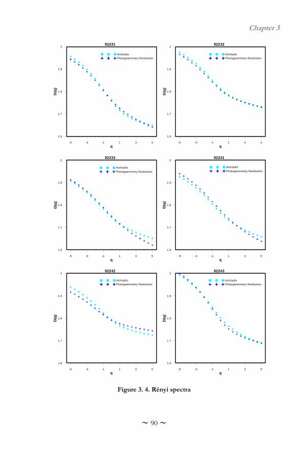
Chapter 3

~ 90 ~ 

 

Figure 3. 4. Rényi spectra

 

-5 -3 -1 1 3 5

q

1.6

1.7

1.8

1.9

2

D(q

)ArcHydroPhotogrammetry Restitution

92231

-5 -3 -1 1 3 5

q

1.6

1.7

1.8

1.9

2

D(q

)

ArcHydroPhotogrammetry Restitution

92232

-5 -3 -1 1 3 5

q

1.6

1.7

1.8

1.9

2

D(q

)

ArcHydro

Photogrammetry Restitution

92233

-5 -3 -1 1 3 5

q

1.6

1.7

1.8

1.9

2

D(q

)ArcHydro

Photogrammetry Restitution

92241

-5 -3 -1 1 3 5

q

1.6

1.7

1.8

1.9

2

D(q

)

ArcHydroPhotogrammetry Restitution

92242

-5 -3 -1 1 3 5

q

1.6

1.7

1.8

1.9

2

D(q

)

ArcHydroPhotogrammetry Restitution

92243

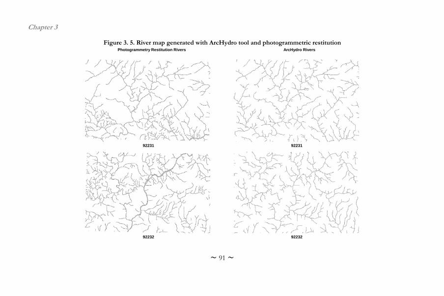
Chapter 3

~ 91 ~ 

 

Figure 3. 5. River map generated with ArcHydro tool and photogrammetric restitution Photogrammetry Restitution Rivers ArcHydro Rivers

92231 92231

9223292232

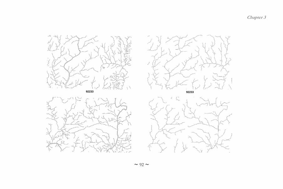
Chapter 3

~ 92 ~ 

 

 

92233 92233

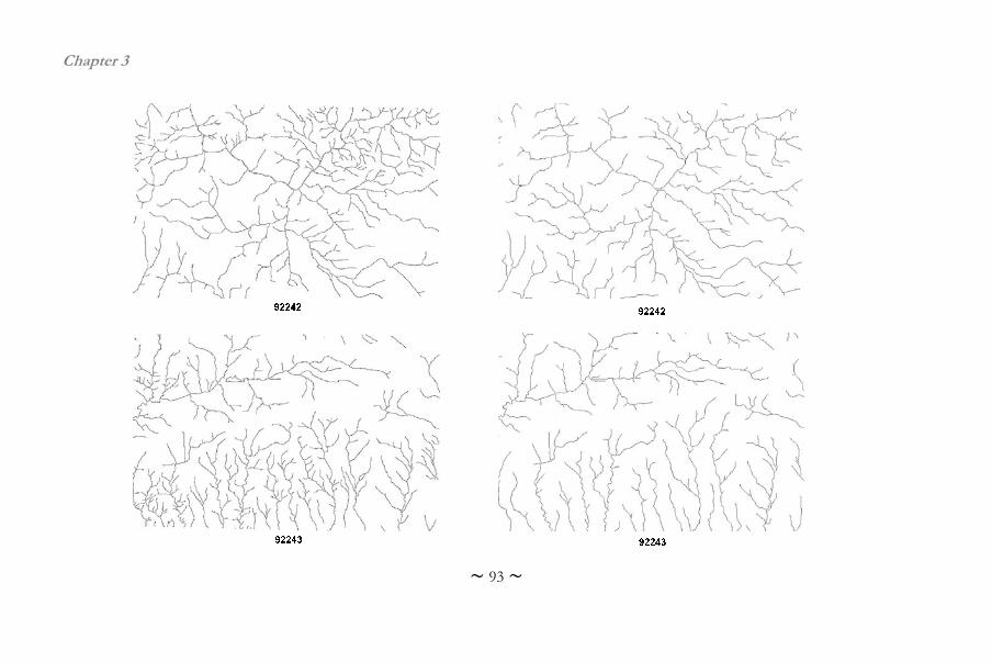
Chapter 3

~ 93 ~ 

 

 

Chapter 3

~ 94 ~ 

 

Correlation dimension D2 describes the uniformity of the river network density among several selected zones (circles of radius R). It describes the probability of finding pixels belonging to the object within a given distance when starting on a pixel belonging to the object. In accordance to the D2

values list in Table 3. 2 it can not to be obtained any information about the uniformity of the imagines distribution due to the values obtained for ArcHydro and photogrammetric restitution are similar.

D0 is the fractal dimension and it refers to the degree of filling space by

river networks. It can be verified in Table 3. 2 that all drainage networks provided from photogrammetric restitution have a higher degree of filling space, meaning that these networks have a greater density of streams than those generated by ArcHydro. Therefore, ArcHydro provides fewer populated networks with a lower number of channel orders.

4. Conclusions

Factors such as DEM resolution, algorithm of stream derivation, cartographic smoothing of the cell-to-cell vector lines and the flow accumulation threshold value have an influence on the accuracy of drainage networks extracted from DEMs by ArcHydro and give wrong results when different features of the hydrological processes are analyzed. As a consequence, this work explores the appropriate selection of the flow accumulation threshold value by using multifractal analysis.

The river networks studied in this research are of a multifractal nature and, consequently, Rényi spectra can be regarded as being an efficient tool for determining the above mentioned threshold value in order to obtain the required detail level. The suitability of ArcHydro river networks has been frequently determined by a visual comparison with those derived from cartographic products such as topographic maps. In this research, the multifractal analysis has been applied as a pattern recognition tool allowing a numerical verification of the resemblance between ArcHydro and photogrammetric restitution river networks. This analysis

Chapter 3

~ 95 ~ 

 

takes advantage of having parameters that are independent over a range of scales. According to the multifractal spectra, the main difference between the networks considered here is the lesser stream density with a low channel order detected for ArcHydro results compared to photogrammetric restitution. However, according to the results obtained, the drainage networks simulated here by ArcHydro are fit to be considered as input data for performing different research and works.

Chapter 3

~ 96 ~ 

 

References

Alexander, R.B., Smith, R.A. & Schwarz, G.E. (2000). Effect of stream

channel size on the delivery of nitrogen to the gulf of Mexico. Nature, 403, 758 – 761.

Costa-Cabral, M., & Burges, S. J. (1994). Digital elevation model networks

(DEMON): A model of flow over hillslopes for computation of contributing and dispersal areas. Water Resour. Res., 30, 1681 – 1692.

Davis, A., Marshak, A., Wiscombe, W., & Cahalan, R. (1994). Multifractal

characterization of non stationarity and intermitency in geophysical fields: observed, retrieved or simulated. J. Geophys. Res., 99, 8055 – 8072.

De Bartolo, S.G., Gaudio, L., & Gabriele, S. (2004). Multifractal analysis of

river network: Sandbox approach. Water Resour. Res., 40, W02201. DOI: 10.1029/2003WR002760.

De Bartolo, S.G., Grabiele, S., & Gaudio, R. (2000). Multifractal behaviour

river networks. Hydrol. Earth Syst. Sci., 4,105 – 112. De Bartolo, S.G., Veltri, M., & Primavera, L. (2006). Estimated generalized

dimensions of river networks. Journal of Hydrology, 322, 1 – 191. Delgado, J., Nieto, J.M., & Boski, T. (2010). Analysis of the spatial variation

of heavy metals in the Guadiana estuary sediments (SW Iberian Peninsula) based on GIS- mapping Techniques. Estuar. Coast Shelf S., 1, 71 – 83.

Dombrádi, E, Timár, G, Bada, G, Cloetingh, S, & Horváth, F. (2007).

Fractal dimension estimations of drainage network in the Carpathian-Pannomian system. Global Planet Change, 58, 197 – 213.

Chapter 3

~ 97 ~ 

 

Falconer, K. J. (1990). Fractal Geometry: Mathematical Foundations and

Applications.( 2nd ed). Chichester: John Wiley. Freeman, T. G. (1991). Calculating Catchment Area with Divergent Flow

Based on a Regular Grid. Comp. Geosci., 17, 413 – 422. Gallant, .J.C., & Wilson, J.P. (1996). Tapes-g: a grid-based terrain analysis

program for the environmental sciences. Comp. Geosci., 22, 713 – 722. Gaudio, R., De Bartolo, S.G., Primavera, L., Grabiele, S., & Veltri. M.

(2005). Lithologic control on the multifractal spectrum of river networks. J. Hydrol., 327, 365 – 375.

Hentschel, H.G.E., & Procaccia, I. (1983). The Infinite number of

generalized dimensions of fractals and strange attractors. Phys. D, 8, 435 − 444.

Jasiewicz, J., & Metz, M. (2011). A new GRASS GIS toolkit for hortonian

analysis of drainage networks. Comput. Geosci., 8, 1162 − 1173. Lea, N. L. (1992). An aspect driven kinematic routing algorithm, in

Overland Flow: Hydraulics and Erosion Mechanics. Chapman and Hall: New York.

Maidment, D.R. (2002). ArcHydro: GIS for Water Resources. Redlands:

ESRI Press. Makaske, B., Smith, D.G., Berendsen, H.J.A., Boer, A.G., Van Nielen-

Kiezebrink, M.F., Locking, T. (2009). Hydraulic and sedimentary processes causing anastomosing morphology of the upper Columbia river, British Columbia, Canada. Geomorphology, 111, 194 − 205.

Chapter 3

~ 98 ~ 

 

Mantilla, R., & Gupta, V.K. (2005). A GIS numerical framework to study the process basis of scaling statistics in river networks. IEEE Geosci. Remote Sens. Lett., 4, 404 − 408.

Mark, D.M. (1984). Automatic detection of drainage networks from digital

elevation models. Cartographica, 21, 168 – 178. Martz, L.W., & Garbrecht, J. (1998). The treatment of flat areas and

depressions in automated drainage analysis of raster digital elevation models. Hydrol. Process., 12, 843 – 855.

Morris, D.G., & Heerdegen, R.G. (1988). Automatically derived catchment boundaries and channel networks and their hydrological applications. Geomorphology, 1, 131 − 141.

Muller, J., Huseby, O.K., & Saucie, A. (1995). Influence of multifractal

scaling of pore geometry on permeabilities of sedimentary rocks. Chaos Solitons Fractals, 5, 1485 – 1492.

Nigel, R., & Rughooputh, S.D.D.V. (2010). Soil erosion risk mapping with

new datasets: an improved identification and prioritisation of high erosion risk areas. Catena, 82, 191 – 205.

O´Callaghan, J., & Mark, D.M. (1984). The extraction of drainage networks

from digital elevation data. Computer Vision Graphics and Image Processing, 3, 323 – 344.

Porter, M.D., & Massong, T.M. (2004). Analyzing changes in river channels

morphology using GIS for Rio Grande silvery minnow habitat assessment. GIS/Spatial Anal Fishery Aquat Sci, 505, 433 – 446.

Prosser, P.I., Rutherfurd, I.D., Olley, J., Young, W.J., Wallbrink, P.J., &

Moran, C.J. (2001). Large-scale patterns of erosion and sediment transport in river networks, with examples from Australia. Mar. Freshw. Res., 52, 81 – 99.

Chapter 3

~ 99 ~ 

 

Ramos, J., & Gracia, J. (2011). Spatial–temporal fluvial morphology analysis in the Quelite river: It’s impact on communication systems. J. Hydrol. DOI:10.1016/j.jhydrol.2011.05.007.

Rhoades, E.L., O'Neala, M.A., & Pizzuto, J.E. (2008). Quantifying bank

erosion on the South River from 1937 to 2005 and its importance in assessing Hg contamination. Appl. Geogr., 1, 125 – 134.

Rinaldo, A., Rodrigueziturbe, I., Rigon, R., Ijjaszvasquez, E., & Bras, R.L.

(1993). Self-organized fractal river networks. Phys. Rev. Lett., 70, 822 –825.

Rodriguez-Iturbe, I., & Rinaldo, A. (1997). Fractal River Networks: Chance

and Self-Organization. New York: Cambridge University Press. Saa, A., Gasco, G., Grau, J.B., Anton, J.M., & Tarquis, A.M. (2007).

Comparison of gliding box and box counting methods in river network analysis. Nonlinear Process Geophys., 14, 603 – 613.

Siber, R., Stamma, C., & Reichert, P. (2009). Modeling potential herbicide

loss to surface waters on the Swiss plateau. J. Environ. Manage., 1, 290 – 302.

Tarboton, D.G. (1997). A new method for the determination of flow

directions and upslope areas in grid digital elevation models. Water Resour. Res., 33, 309 – 319.

Tél, T., Fülöp, Á., & Vicsek, T. (1989). Determination of fractal dimensions

for geometrical multifractals. Phys. A, 159, 155 – 166. Terrado, M., Barceló, D., & Tauler, R. (2006). Identification and

distribution of contamination sources in the Ebro river basin by chemometrics modelling coupled to geographical information systems. Talanta, 70, 691 – 704.

Chapter 3

~ 100 ~ 

 

Turcotte, R., Fortin, J.-P., Rousseau, A.N., Massicotte, S., & Villeneuve, J.-P. (2001). Determination of the drainage structure of a watershed using a digital elevation model and a digital river and lake network. J. Hydrol., 240, 225 – 242.

Veneziano, D., Moglem, G.E., & Bras, R.L. (1995). Multifractals analysis:

Pitfalls of standard procedures and alternatives. Phys. Rev. E, 25, 1387 – 13898.

Vicsek, T., Family, F., & Meakin, P. (1990). Multifractal geometry of

diffusion- limited aggregates. Europhys. Lett., 12, 217 – 222. Vicsek, T. (1990). Mass multifractal. Phys. A, 168, 490 – 497. Vital, H., Stattegger, K., Posewang, J., & Theilen, F. (1998). Lowermost

Amazon River: morphology and shallow seismic characteristics. Mar. Geol. 152, 277 – 294.

Wagenschein, D., & Rode, M. (2008). Modelling the impact of river

morphology on nitrogen retention- A case study of the Weisse Elster River (Germany). Ecol. Model., 2, 224 – 232.

Winterbottom, S.J., & Gilvear, D.J. (2000). A Gis-based approach to

mapping probabilities of river bank erosion: regulated River Tummel, Scotland. Regul River, 16, 127 – 140.

 

~ 101 ~ 

 

Chapter 3

~ 102 ~ 

 

Conclusions

“I believe that scientific knowledge has fractal properties: that no matter how much we learn,

whatever is left, however small it may seem. is just as infinitely complex as the whole was to start with.

That, I think, is the secret of the Universe.”

Isaac Asimov (1920-1992)

 

~ 103 ~ 

 

Conclusions

 

~ 104 ~ 

 

Conclusions General conclusions

Multifractal nature of different kinds of anthropogenic and natural

networks is studied along this thesis. The algorithm used in this research to study these networks is Sandbox fixed-size method, which overcomes some limitations of Box-Counting fixed-size method when networks are studied. It is explored the use of Sandbox approach to analyse variables in three dimensions and it is compared with Box-Counting method. The latter method produces higher standard error than Sandbox algorithm when multifractal spectrum is calculated, providing more accurate results and describing variables in a more efficient way.

Multifractality is evident in the case of irregular networks

morphologies, being needed a set of fractal dimensions to describe their complexity and, as consequence, the self-similarity are going to depend on the scale. On the other hand, it should be noted that the fractal nature, in the case of regular networks morphologies, is defined by a single fractal dimension.

The Rényi or Generalized Dimension Spectrum is used in this

work as the key to determine the fractal or multifractal nature of networks. When the different values for fractal dimensions Dq display a strong dependence for all analyzed moment orders or q values, the studied data exhibit a multifractal nature (case of irregular networks); the opposite case occurs in fractal nature wherein Dq values are the same for all analyzed moment orders values.

Conclusions

 

~ 105 ~ 

 

Multifractal analysis can be considered as a tool to check models validity: if a phenomenon exhibits a multifractal nature, this one has to be present in simulate results.

Chapters conclusions

The conclusions listed below are obtained through the different chapters of this thesis:

i. The Sandbox algorithm improves the performances of multifractal analysis carried out with the Box-Counting procedure due to the reduction of undesired effects of anomalous contribution in regions containing few data points within the calculation of the generalized fractal dimension (Chapter 1).

ii. The fractal dimension obtained with Sandbox method, when networks are studied in 3D, is lower (D0) than the geometric support of measure. This circumstance determines the influence of pore phase geometry on flows that cannot fill the 3D domain (Chapter 1).

iii. The multifractal spectra estimated with Sandbox method indicate the influence of the porous media structure on simulated flows in a clearer way. As porosity increase, the method reveals more uniformity in the distribution of flow velocity values (Chapter 1).

iv. Multifractal analysis reveals the existence of multifractal nature in some urban areas, especially when dealing with irregular urban pattern. Thereby, these areas cannot be described by a single fractal dimension as previous research states, being the parameters of Rényi spectra

Conclusions

 

~ 106 ~ 

 

enough to characterize irregular networks morphologies. (Chapter 2).

v. Multifractal analysis shows to be an efficient pattern recognition tool, contrasting the differences between images. Multifractal analysis detects that ArcHydro tool generates lesser stream density with low channel order (Chapter 3).

vi. Rényi spectrum can be regarded as an efficient tool for determining the flow accumulation threshold value when networks are generated from a Digital Terrain Model by ArcHydro tool (Chapter 3).

 

~ 107 ~