1.0 analysing open-ended survey question data in caqdas
TRANSCRIPT

Analysing OEQs in NVivo v8
CAQDAS Networking Project © Graham Hughes, Christina Silver & Ann Lewins QUIC Working Paper #015
1.0 Analysing Open-Ended Survey Question Data in CAQDAS Packages: Data Preparation for NVivo (v7 & v8) The following material provides step-by-step guidance for preparing the texts, collected from a large number of respondents answering several open-ended questions in a survey situation, for qualitative analysis using NVivo software. These instructions assume that the decision has been made to organise these texts into a separate document for each question, with many respondents included in each document. (For a discussion of the arguments for and against such a decision please see the material here). This way of organising the data is not the mainstream procedure in NVivo and so these instructions may be seen as a “workaround” to achieve a satisfactory basis for analysis. There are many stages in this procedure, some of which may not be relevant in certain circumstances. Some users may have alternative methods or short-cuts, in which case please use your own judgment as to which elements from these instructions to apply. Our purpose here is to provide a comprehensive guide, which has been tested and proved to work, for the benefit of those who have not achieved this task successfully before. These instructions refer to Microsoft Excel and Microsoft Word and are illustrated with screenshots from those programs, however the operations involved are not particularly sophisticated and any equivalent spreadsheet and word-processing programs would probably be usable as alternatives.
TIP: If you have several batches of response texts to analyse it will be most efficient to repeat each stage for all the batches before moving on to the next step. However, it may also be a good idea to take the first batch right through the whole process to make sure that it is working correctly with your data and software versions before committing the time to process all batches.
Outline
1.1 Locate the set of response texts and a unique identifier (ID) for each respondent and copy
them into Microsoft Excel.
1.2 If necessary, reformat the IDs.
1.3 Export the response texts and IDs to Microsoft Word for formatting.
1.4 Select the socio-demographic attribute variables that will be required to be available in
NVivo to inform the qualitative analysis and copy them into Microsoft Excel.
1.5 Edit the variables in Excel as necessary then save as a Unicode Text file.
1.6 Import the Unicode Text file into the NVivo Casebook, and create the cases.
1.7 Import the response text documents into NVivo and autocode by case IDs.

Analysing OEQs in NVivo v8
CAQDAS Networking Project © Graham Hughes, Christina Silver & Ann Lewins QUIC Working Paper #015
Detailed Steps: 1.1 Locate the set of response texts and a unique identifier (ID) for each respondent and
copy them into Microsoft Excel.
This step may not be necessary if the response texts are already organised in a Microsoft Word document with appropriate identifiers for each respondent, in which case please skip to step 3 and continue from there. If, on the other hand, the texts are being extracted from an SPSS data file or some other database format then this step can be a useful means of organising the data in the first instance.
TIP: Before carrying out any data processing, examine the data in their most original format in order to identify some of the longest individual responses and to look for unusual characters in the texts. The longer responses may get truncated in some conversion processes (for example on being brought into SPSS if the 256 character default was not changed) and it is useful to be able to check that you have the fullest versions before analysis begins. Unusual characters, other than basic alpha-numeric and punctuation, sometimes affect conversion processes so it is a good idea to check that these have been copied faithfully before proceeding.
Create a separate Excel worksheet for each open-ended question, grouped into a single workbook using the sheet name tabs to identify them. Each worksheet should have two columns, one with the unique respondent identifiers, and the other with the response texts. Each row represents an individual respondent. Adjust column widths and use the Word-wrap and Autofit row-height commands (or their equivalent in your spreadsheet program) to display the longest responses in full.
1.2 If necessary, reformat the IDs.
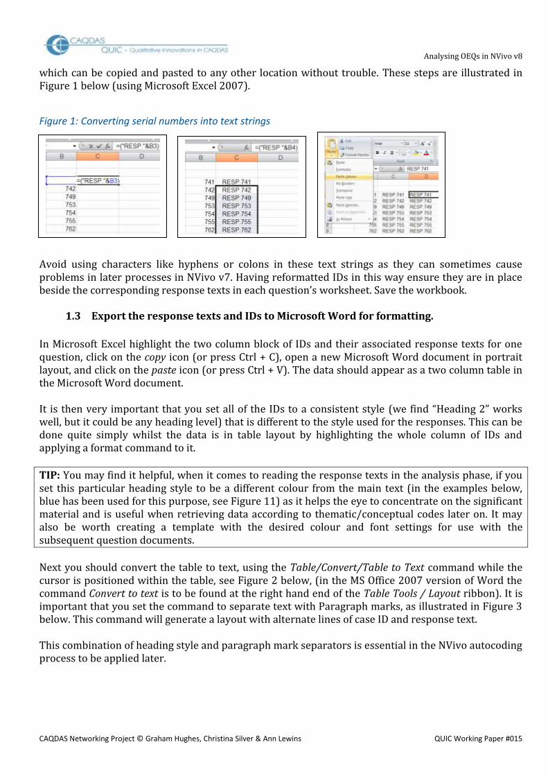
The identifier for each respondent (or “case” in NVivo’s terminology) will be very significant in this process, in order to link the socio-demographic characteristics with the analysis of the responses and later to link the responses to different questions made by each speaker. Therefore careful thought about identifiers will be helpful at this point. Each separate response must have some means of identifying the respondent who made it. Generally in quantitative surveys there will be a serial number, not necessarily in a completely unbroken sequence as it may originate in a sampling procedure, whereas qualitative researchers are more used to using forenames or initials to identify their informants. For the purposes of the sort of analysis envisaged here it is very important that each identifier (ID) is unique and serial numbers are probably more reliable for this purpose. For some later purposes it will be useful if the ID is in the form of a text string, rather than a pure number, so it is important to prefix the serial numbers with a few letters, such as “RESP”. This can be done quite simply in Microsoft Excel by using the concatenation function, as illustrated below. If cell B3 has a serial number in it (say 741), in cell C3 type the following logic: =(“RESP.0”&B3) Cell C3 will then display the result as RESP.0741 and this may be copied down the column as many times as necessary. Finally, the whole of column C should be copied and pasted into column D using the Paste Special command set to Paste Values. This removes the underlying logic and stores the strings as pure text
Analysing OEQs in NVivo v8
CAQDAS Networking Project © Graham Hughes, Christina Silver & Ann Lewins QUIC Working Paper #015
which can be copied and pasted to any other location without trouble. These steps are illustrated in Figure 1 below (using Microsoft Excel 2007).
Figure 1: Converting serial numbers into text strings Avoid using characters like hyphens or colons in these text strings as they can sometimes cause problems in later processes in NVivo v7. Having reformatted IDs in this way ensure they are in place beside the corresponding response texts in each question’s worksheet. Save the workbook.
1.3 Export the response texts and IDs to Microsoft Word for formatting.
In Microsoft Excel highlight the two column block of IDs and their associated response texts for one question, click on the copy icon (or press Ctrl + C), open a new Microsoft Word document in portrait layout, and click on the paste icon (or press Ctrl + V). The data should appear as a two column table in the Microsoft Word document. It is then very important that you set all of the IDs to a consistent style (we find “Heading 2” works well, but it could be any heading level) that is different to the style used for the responses. This can be done quite simply whilst the data is in table layout by highlighting the whole column of IDs and applying a format command to it.
TIP: You may find it helpful, when it comes to reading the response texts in the analysis phase, if you set this particular heading style to be a different colour from the main text (in the examples below, blue has been used for this purpose, see Figure 11) as it helps the eye to concentrate on the significant material and is useful when retrieving data according to thematic/conceptual codes later on. It may also be worth creating a template with the desired colour and font settings for use with the subsequent question documents.
Next you should convert the table to text, using the Table/Convert/Table to Text command while the cursor is positioned within the table, see Figure 2 below, (in the MS Office 2007 version of Word the command Convert to text is to be found at the right hand end of the Table Tools / Layout ribbon). It is important that you set the command to separate text with Paragraph marks, as illustrated in Figure 3 below. This command will generate a layout with alternate lines of case ID and response text. This combination of heading style and paragraph mark separators is essential in the NVivo autocoding process to be applied later.

Analysing OEQs in NVivo v8
CAQDAS Networking Project © Graham Hughes, Christina Silver & Ann Lewins QUIC Working Paper #015
Figure 2: Convert table to text (Microsoft Office 97-2003 version)
Figure 3: Set separators to paragraph marks
Save the file as a Microsoft Word document, locating it in the directory where the rest of your project data is stored, and using a short name that unambiguously identifies the question to which the responses belong. This name will be used by NVivo as the source name once the file has been imported.

Analysing OEQs in NVivo v8
CAQDAS Networking Project © Graham Hughes, Christina Silver & Ann Lewins QUIC Working Paper #015
1.4 Select the socio-demographic attribute variables that will be required to be available
in NVivo to inform the qualitative analysis and copy them into Microsoft Excel.
This step is similar to the first in some respects but contains the attributes of the respondents which may be relevant to the subsequent analysis. It is quite possible to add further attributes for all respondents during the analysis, so the decision over which attributes to include at this point is not an irrevocable one with NVivo.
TIP: However it is worth making sure that you use all of the data that you can reasonably expect to consider during the analysis, as it is easier to incorporate it at this stage.
For further comments and guidance on selecting variables to use in such analysis please see the notes here. It is quite likely that the variable data is available to you in a statistical program like SPSS, in which case there is a straightforward procedure for transferring the data to Microsoft Excel. However, before you start the transfer it may be worth considering doing some recoding within SPSS in order to simplify the variables. It is possible to alter some strings in Microsoft Excel, by using “find and replace” commands, but it is certainly easier and less error prone to do this in SPSS. In SPSS terminology, it is the “Value Labels” that you will be exporting and so these are the items that need to be made short and clear. The number of different values each variable can take may be significant so reducing these by grouping some together may be helpful. Again, more guidance is given on this page. The procedure for exporting data from SPSS to Excel uses the Save As command in SPSS.
TIP: It can be done in a single step but a two stage process provides a mid-point to return to if something goes wrong.
Having completed the selection and recoding decisions and processes and saved the full dataset, start the Save as command to create a new data file with all of the cases but only the particular variables that are wanted for analysis in NVivo. Click on the Variables button to open the dialogue screen that allows you to select a subset of the variables into a new dataset. It will probably be best to click on the Drop All button first, to uncheck every variable box, and then manually tick the box for each variable that you have decided to use (in its recoded form if you made that a new variable). Make sure that you include the ID or serial number variable in the list. When this selection operation is complete, click on the Continue button, enter an appropriate new name and path for the file to be stored at (you don’t want to overwrite the master data file and thus delete valuable data), leave the file type as “*.sav”, and save the file. Now open the new data file that you have just created in SPSS and close the master data file (which will still be open if you are using SPSS v15 or higher), and check that you have all of the data that you expect to bring into NVivo. If necessary repeat the last steps to correct any omissions or errors. When you are satisfied that all is correct, start another Save as command. This time on the main dialogue screen change the Save as type field to “Excel 97 through 2003 (*.xls)” by using the drop-down menu. When this is selected, two further options below come into use. You should tick both of them – Write variable names to spreadsheet and Save value labels where defined instead of data values. The first of these will provide helpful identification of each attribute as column headers in Microsoft Excel, the
Analysing OEQs in NVivo v8
CAQDAS Networking Project © Graham Hughes, Christina Silver & Ann Lewins QUIC Working Paper #015
second makes sure that you can interpret the attribute in a qualitative environment (“Mother” makes more sense than “1”). Finally enter a file name, which can be similar to the one used for the temporary SPSS file because it will have a different extension (.xls instead of .sav) and hit the Save button. (If you have Microsoft Office 2007 available you can use that version to save to “*.xlsx”).
1.5 Edit the variables in Excel as necessary then save as a Unicode Text file.
Using Microsoft Excel, open the file that you have just created. It is very important that the case IDs in this file exactly match those used in the response text documents. So, if you reformatted the serial numbers as ID strings for the response text documents, you will need to repeat the process (from step 2 above) here so that the IDs in the Casebook can be connected to the IDs in the response texts.
TIP: You may find it helpful to edit the variable names, which appear at the top of each column, to be more easily interpreted within NVivo later. Check also that the value labels for each variable are simple, clear, and as short as possible. Both the variable and value names can be edited with the Find and replace command if necessary.
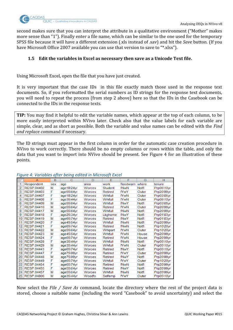
The ID strings must appear in the first column in order for the automatic case creation procedure in NVivo to work correctly. There should be no empty columns or rows within the table, and only the data that you want to import into NVivo should be present. See Figure 4 for an illustration of these points.
Figure 4: Variables after being edited in Microsoft Excel
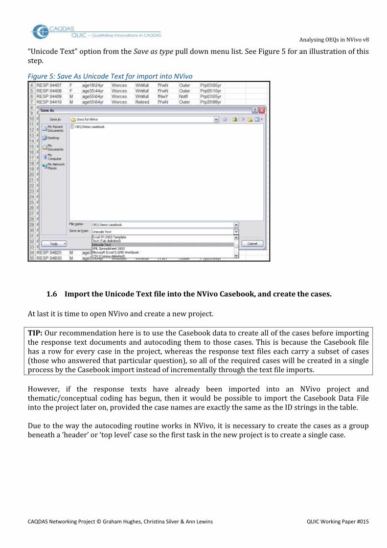
Now select the File / Save As command, locate the directory where the rest of the project data is stored, choose a suitable name (including the word “Casebook” to avoid uncertainty) and select the
Analysing OEQs in NVivo v8
CAQDAS Networking Project © Graham Hughes, Christina Silver & Ann Lewins QUIC Working Paper #015
“Unicode Text” option from the Save as type pull down menu list. See Figure 5 for an illustration of this step.
Figure 5: Save As Unicode Text for import into NVivo
1.6 Import the Unicode Text file into the NVivo Casebook, and create the cases.
At last it is time to open NVivo and create a new project.
TIP: Our recommendation here is to use the Casebook data to create all of the cases before importing the response text documents and autocoding them to those cases. This is because the Casebook file has a row for every case in the project, whereas the response text files each carry a subset of cases (those who answered that particular question), so all of the required cases will be created in a single process by the Casebook import instead of incrementally through the text file imports.
However, if the response texts have already been imported into an NVivo project and thematic/conceptual coding has begun, then it would be possible to import the Casebook Data File into the project later on, provided the case names are exactly the same as the ID strings in the table. Due to the way the autocoding routine works in NVivo, it is necessary to create the cases as a group beneath a ‘header’ or ‘top level’ case so the first task in the new project is to create a single case.

Analysing OEQs in NVivo v8
CAQDAS Networking Project © Graham Hughes, Christina Silver & Ann Lewins QUIC Working Paper #015
Figure 6: Create Header Case in NVivo project
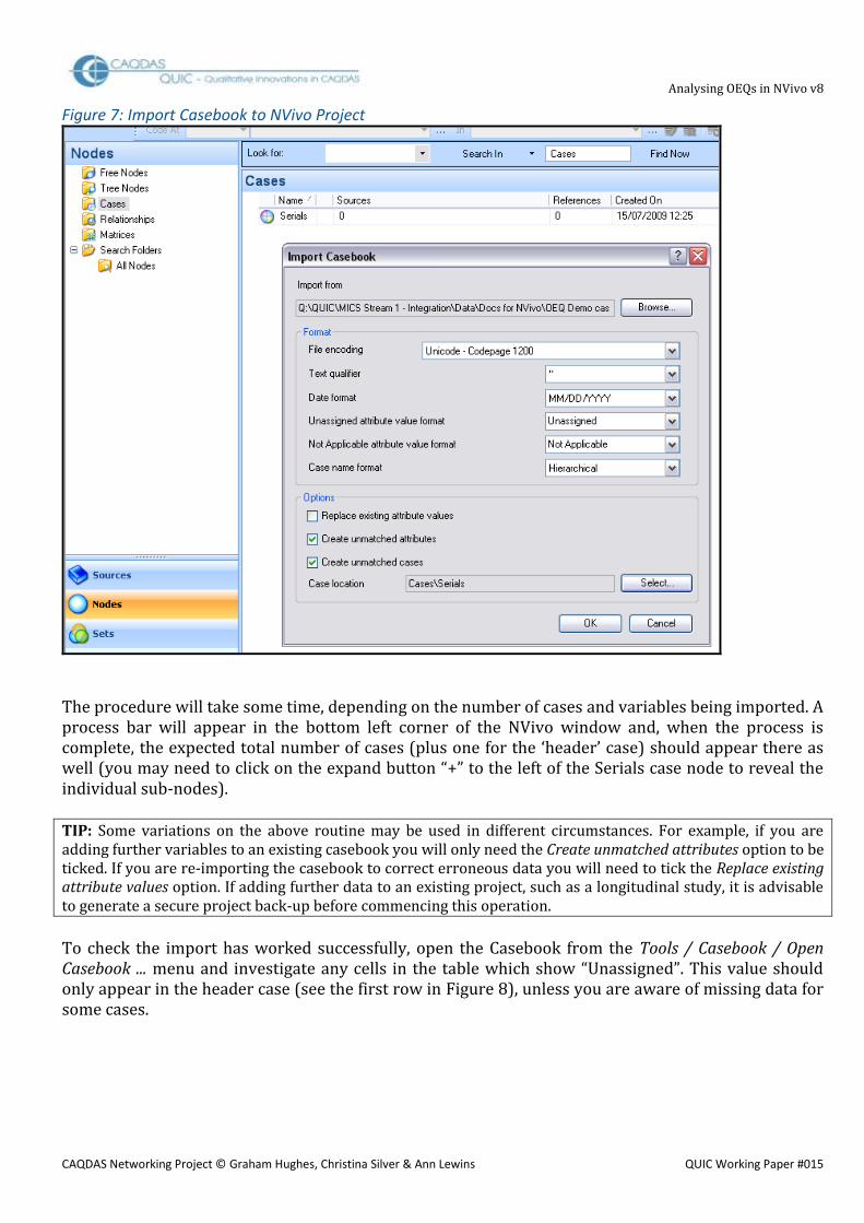
In the navigation pane, select Nodes and then choose the Cases subfolder. From the New drop-down menu, select New Case in This Folder to open the New Case dialogue box (Figure 6). Enter a name for the set of cases into the Name field, in this example we used “Serials”. No other entries are absolutely necessary in this dialogue box, so hit OK. Select Tools / Casebook / Import Casebook ... from the Main Menu to open the dialogue illustrated in Figure 7. Using the Browse button, locate the Unicode Text file that you created at the end of step 5 for the Import from field. There should be no need to alter the defaults in the format fields. For the three fields under the heading Options, ensure that Create unmatched attributes and Create unmatched cases are checked, but leave the first one blank because there should be no existing attribute values in a new project. Finally, and most importantly, the Case location field needs to be set to the name of the single case you created in the instruction above by using the Select button, in our example it is “Cases/Serials”. It is necessary to use some care with this selection dialogue; you have to click on the cases folder in the left hand panel to display the Serials case on the right, where the case node checkbox can be ticked. Only then will the OK button become active and return you to the main dialogue box, where you should confirm that the field correctly displays the “Cases/Serials” path, before clicking the final OK to effect the whole import command.
Analysing OEQs in NVivo v8
CAQDAS Networking Project © Graham Hughes, Christina Silver & Ann Lewins QUIC Working Paper #015
Figure 7: Import Casebook to NVivo Project
The procedure will take some time, depending on the number of cases and variables being imported. A process bar will appear in the bottom left corner of the NVivo window and, when the process is complete, the expected total number of cases (plus one for the ‘header’ case) should appear there as well (you may need to click on the expand button “+” to the left of the Serials case node to reveal the individual sub-nodes). TIP: Some variations on the above routine may be used in different circumstances. For example, if you are adding further variables to an existing casebook you will only need the Create unmatched attributes option to be ticked. If you are re-importing the casebook to correct erroneous data you will need to tick the Replace existing attribute values option. If adding further data to an existing project, such as a longitudinal study, it is advisable to generate a secure project back-up before commencing this operation.
To check the import has worked successfully, open the Casebook from the Tools / Casebook / Open Casebook ... menu and investigate any cells in the table which show “Unassigned”. This value should only appear in the header case (see the first row in Figure 8), unless you are aware of missing data for some cases.

Analysing OEQs in NVivo v8
CAQDAS Networking Project © Graham Hughes, Christina Silver & Ann Lewins QUIC Working Paper #015
Figure 8: Check NVivo Casebook
Note how similar this is to the Microsoft Excel spreadsheet. However, NVivo has altered the order of the variables so that the columns appear in alphabetical order according to the variable names. Save the project.
1.7 Import the response text documents into NVivo and autocode by case IDs.
The text documents are imported into NVivo’s Sources area within the “Internals” folder in the same way as interview transcripts would be. Click on Sources and then Internals in the navigation panel. Then select the command Project / Import Internals from the Main Menu bar. This brings up a dialogue screen like the one shown in Figure 9. Click on the Browse button to open a standard navigation dialogue and use it to locate the files that you created at step 3 above. It is possible to import several files at the same time by using the shift or control keys with the mouse clicks. Of the three supplementary questions in this dialogue screen we recommend that you tick the first and third but not the second. When importing files one at a time, ticking the text option to Create descriptions will cause the program to prompt you to fill in a description field in the properties box for each NVivo source (it is a good idea to include the full text of the question that was used to generate the responses in each file as part of this description). If importing multiple files simultaneously, ticking this option will automatically create source descriptions by turning the first paragraph of each file into the corresponding source description. You do not want to code these sources as new cases because you have structured them to contain many cases, so leave that option blank. The final option, to Create as read-only is recommended in order to protect the response texts from accidental alteration – it does not affect coding operations. Click on OK to effect the import command.

Analysing OEQs in NVivo v8
CAQDAS Networking Project © Graham Hughes, Christina Silver & Ann Lewins QUIC Working Paper #015
Figure 9: Import documents into NVivo Project
The next step, the autocode routine, can be carried out separately for each source or for several sources together. Within Sources / Internals, click on a single source to highlight it, or multiple sources using the shift or control keys, and then select the command Code / Auto Code... to open the dialogue screen shown in Figure 10 (note its icon which can be found towards the right end of the coding toolbar – and is highlighted in yellow near the top right corner of Figure 10). This is the point at which the heading style, which you applied to the respondents’ IDs at step 3 above, becomes relevant. In our example we used “Heading 2” to format the IDs so that option has to be moved into the right-hand box as the selected paragraph style. It is then important to get the correct settings for Code at Nodes. All of the cases have already been created in step 6 above, so you need the Existing Node setting, and the dialogue behind the select button here works similarly to the one used to create those cases in step 6 above although the screen display (when you have selected the correct header case as before) is subtly different as can be seen if you compare Figure 7 and Figure 10. Click the OK button to effect the command and watch the green processor bar display. When the process has completed you should see the number of responses in the question document appear in both the Nodes and References columns in the top half of the main window. In the example shown in Figure 10, the first seven documents have already been autocoded and so the numbers of Nodes and References contained in each source are listed in the adjacent columns, whereas the final document (“QVAL2”) is about to be processed.

Analysing OEQs in NVivo v8
CAQDAS Networking Project © Graham Hughes, Christina Silver & Ann Lewins QUIC Working Paper #015
Figure 10: Auto Code the response documents by Cases
TIP: A final check on the success of the autocoding process can be made by opening a document, turning on the coding stripes to “Nodes Recently Coding”, and scrolling to the bottom of the document. This should display something like Figure 11 at which point you can confirm that the coding stripes do not overlap, so that every part of the document has been coded to exactly one case.

Analysing OEQs in NVivo v8
CAQDAS Networking Project © Graham Hughes, Christina Silver & Ann Lewins QUIC Working Paper #015
Figure 11: Check Coding Stripes
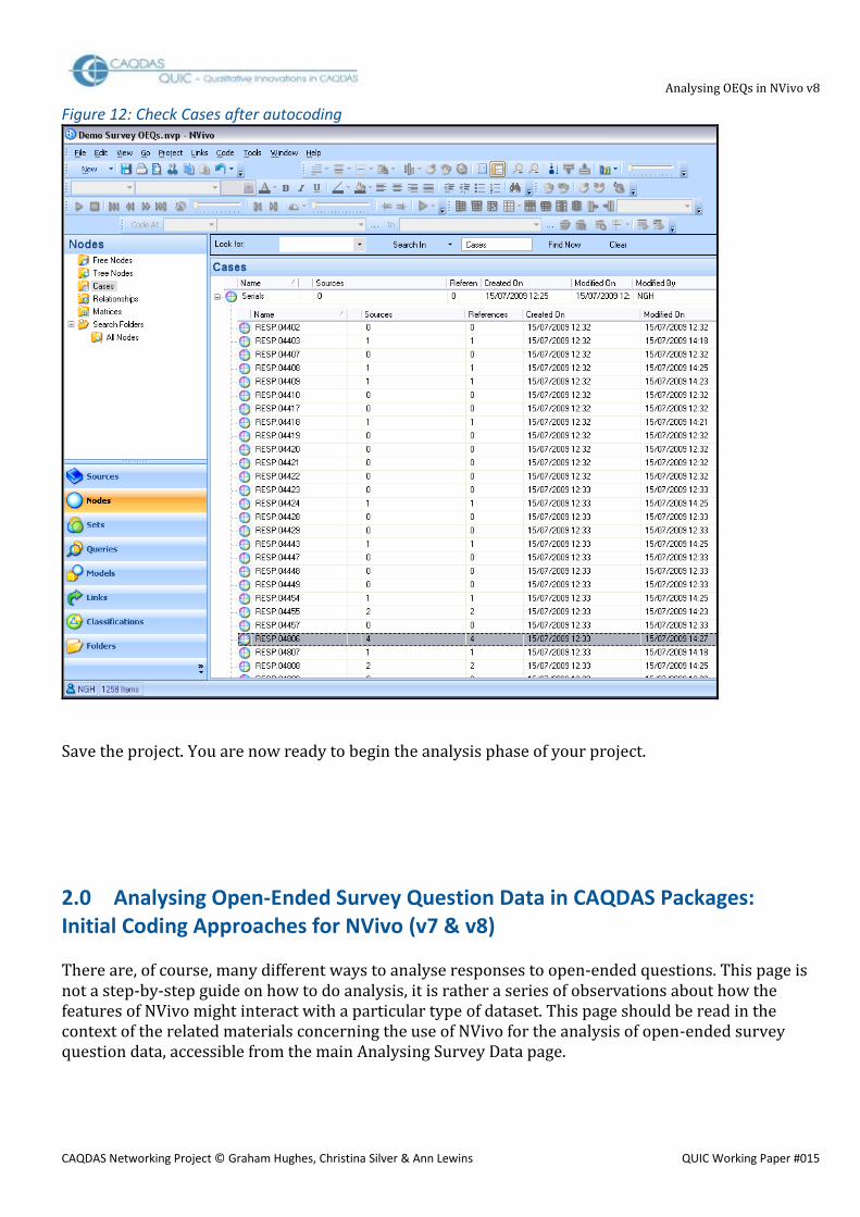
TIP: If you open the Cases folder within Nodes and click on the expand “+” button beside the header case (“Serials” in our example) you should be able to see the beginning of your full list of respondents. The number appearing in each row beneath “Sources” and “References” indicates the number of questions answered by that respondent. In Figure 12 it can be seen that respondent number 04806 has answered 4 questions of the 8 used in this example.
Analysing OEQs in NVivo v8
CAQDAS Networking Project © Graham Hughes, Christina Silver & Ann Lewins QUIC Working Paper #015
Figure 12: Check Cases after autocoding
Save the project. You are now ready to begin the analysis phase of your project.
2.0 Analysing Open-Ended Survey Question Data in CAQDAS Packages: Initial Coding Approaches for NVivo (v7 & v8)
There are, of course, many different ways to analyse responses to open-ended questions. This page is not a step-by-step guide on how to do analysis, it is rather a series of observations about how the features of NVivo might interact with a particular type of dataset. This page should be read in the context of the related materials concerning the use of NVivo for the analysis of open-ended survey question data, accessible from the main Analysing Survey Data page.

Analysing OEQs in NVivo v8
CAQDAS Networking Project © Graham Hughes, Christina Silver & Ann Lewins QUIC Working Paper #015
The tools discussed below are illustrated with examples from the same post flooding event survey that was used to illustrate the data preparation processes. For a summary of the project from which this data derives see here. This data is characterised by a fairly large number of short statements.
Summary: 2.1 Reading the texts – by respondent or by question?
2.2 Developing a coding scheme – manually or by using word frequency tools?
2.3 Text finding, searching and autocoding.
2.4 Coding – data indexing versus data reduction.
2.5 Checking summarising codes – consistency and omissions.
2.6 Looking for similarities or differences?
Details: 2.1 Reading the texts – by respondent or by question?
It is possible in NVivo to work with the survey responses in either presentation – all the answers given by each respondent in turn, or all of the responses to one question at a time. However, depending on the way the data was formatted before being imported, one way will be much easier to implement than the other. Please see this page for a discussion of the advantages and disadvantages of each view in various circumstances. If the data has been formatted and imported in the way suggested by the data preparation instructions on this site then it will be a simple matter to click on Source / Internals and double click on a document name to see all of the responses to that one question in the Detailed View pane. This layout lends itself to the process of reading and coding those responses to themes taken from the data itself. The texts in the Detail View pane can be scrolled easily to move forwards and backwards through the data for that question. The respondent who has provided each answer should be clearly visible through the format in which the data was prepared (see Figure 13 for an illustration of this layout).

Analysing OEQs in NVivo v8
CAQDAS Networking Project © Graham Hughes, Christina Silver & Ann Lewins QUIC Working Paper #015
Figure 13: A basic working screen layout in NVivo 8 showing the responses to one question
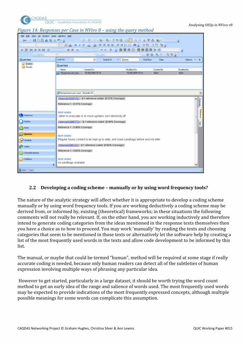
Even when the data has been grouped by question it is still possible to view the data grouped by respondent instead. Select Nodes / Cases, then open the full list of cases by clicking on the + button beside the header case, and then double click on a single case ID to see all of their responses in the Detailed View pane. The questions for which responses have been collected are visible as document names just above each separate response. This is illustrated in Figure 14. There is more distracting information in the display than is found with the internal source method at Figure 13, and it takes a certain amount of trouble to generate the display for the next case, so this may prove an unsatisfactory basis for detailed analysis and coding work. TIP: If you find that you often want to look at the data in this way you may find it useful to create and save a Coding Query instead. On the Coding Criteria / Simple tab highlight the “Node” button and then us the “Select” function to navigate to the required case.
Analysing OEQs in NVivo v8
CAQDAS Networking Project © Graham Hughes, Christina Silver & Ann Lewins QUIC Working Paper #015
Figure 14: Responses per Case in NVivo 8 – using the query method
2.2 Developing a coding scheme – manually or by using word frequency tools?
The nature of the analytic strategy will affect whether it is appropriate to develop a coding scheme manually or by using word frequency tools. If you are working deductively a coding scheme may be derived from, or informed by, existing (theoretical) frameworks; in these situations the following comments will not really be relevant. If, on the other hand, you are working inductively and therefore intend to generate coding categories from the ideas mentioned in the response texts themselves then you have a choice as to how to proceed. You may work ‘manually’ by reading the texts and choosing categories that seem to be mentioned in those texts or alternatively let the software help by creating a list of the most frequently used words in the texts and allow code development to be informed by this list. The manual, or maybe that could be termed “human”, method will be required at some stage if really accurate coding is needed, because only human readers can detect all of the subtleties of human expression involving multiple ways of phrasing any particular idea. However to get started, particularly in a large dataset, it should be worth trying the word count method to get an early idea of the range and salience of words used. The most frequently used words may be expected to provide indications of the most frequently expressed concepts, although multiple possible meanings for some words can complicate this assumption.
Analysing OEQs in NVivo v8
CAQDAS Networking Project © Graham Hughes, Christina Silver & Ann Lewins QUIC Working Paper #015
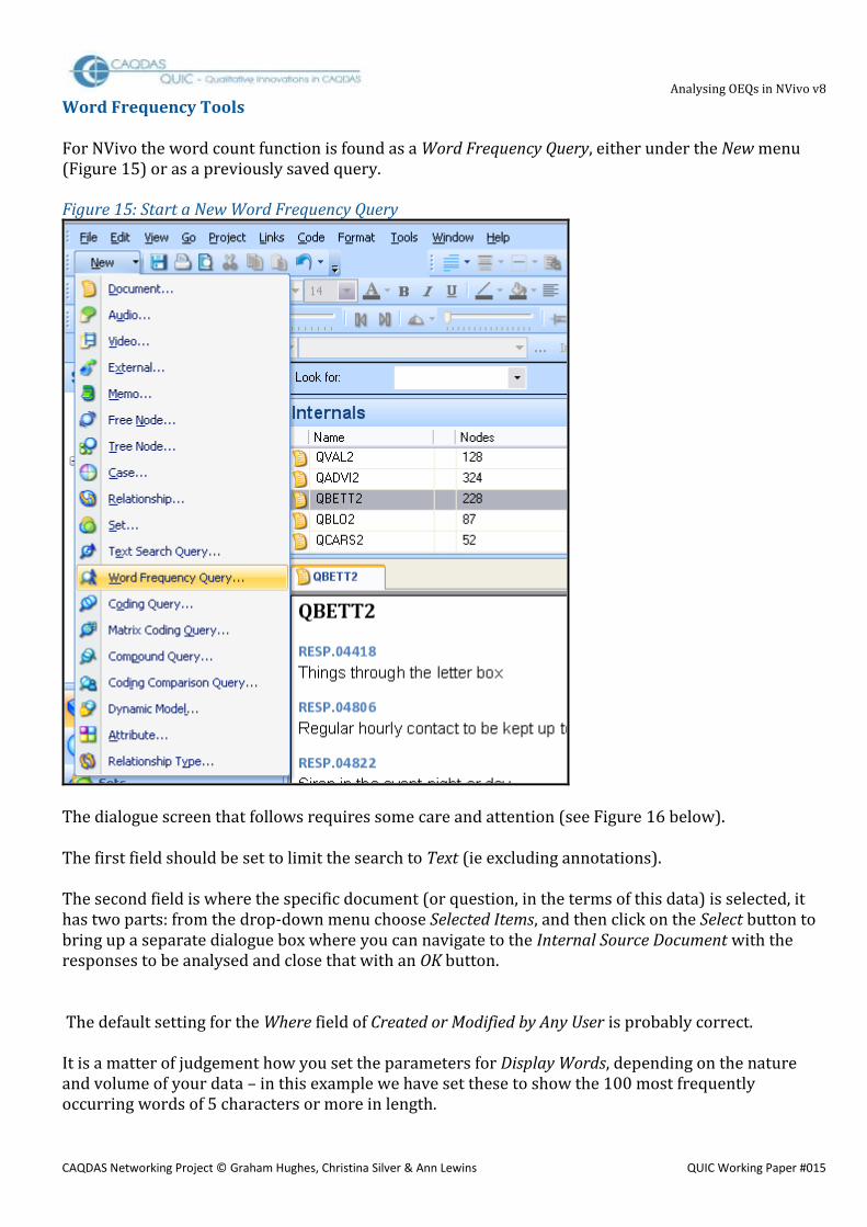
Word Frequency Tools For NVivo the word count function is found as a Word Frequency Query, either under the New menu (Figure 15) or as a previously saved query.
Figure 15: Start a New Word Frequency Query
The dialogue screen that follows requires some care and attention (see Figure 16 below). The first field should be set to limit the search to Text (ie excluding annotations). The second field is where the specific document (or question, in the terms of this data) is selected, it has two parts: from the drop-down menu choose Selected Items, and then click on the Select button to bring up a separate dialogue box where you can navigate to the Internal Source Document with the responses to be analysed and close that with an OK button. The default setting for the Where field of Created or Modified by Any User is probably correct. It is a matter of judgement how you set the parameters for Display Words, depending on the nature and volume of your data – in this example we have set these to show the 100 most frequently occurring words of 5 characters or more in length.

Analysing OEQs in NVivo v8
CAQDAS Networking Project © Graham Hughes, Christina Silver & Ann Lewins QUIC Working Paper #015
TIP: You may need to experiment with a variety of settings for these parameters to find what is most effective with your data, and to make your life easier in that process it may be worth ticking the box to add the query to your project before hitting the Run button for the first time.
Figure 16: Word Frequency Set up
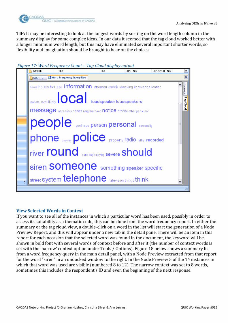
Word Frequency Outputs NVivo has two possible displays of the output from this query, a basic list of words and the number of times they have been found in the selected document, and a “Tag Cloud” where the words are listed in alphabetical order but with font size proportional to their frequency, as illustrated in Figure 17 below. The two presentations can be viewed alternately by clicking on the tabs “Summary” or “Tag Cloud” at the right hand side of the panel. In the Summary presentation (See Figure 18 below) the list can be sorted in ascending or descending order for any of the columns (alphabetical, length or count), controlled by clicking on the column header area. Not all of the results are meaningful as indications of useful concepts, for example the fifth most frequently used word in this illustration (Figure 18) was “would”, used in several different senses of meaning and thus not lending itself to any particular thematic code, so judgement will still be needed to select coding categories, but some useful information can be seen very quickly. This data is about better ways to warn people when a flood is imminent and the prominence of words like “local”, “police” and “telephone” is interesting. Note, also, how “loudspeaker” has been split into two separate words, with its plural version being used sometimes, apparently halving its prominence in the tag cloud.
Analysing OEQs in NVivo v8
CAQDAS Networking Project © Graham Hughes, Christina Silver & Ann Lewins QUIC Working Paper #015
TIP: It may be interesting to look at the longest words by sorting on the word length column in the summary display for some complex ideas. In our data it seemed that the tag cloud worked better with a longer minimum word length, but this may have eliminated several important shorter words, so flexibility and imagination should be brought to bear on the choices.
Figure 17: Word Frequency Count – Tag Cloud display output
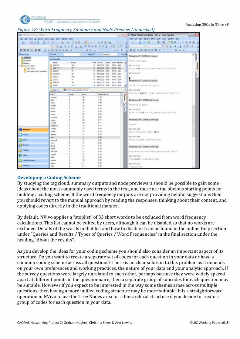
View Selected Words in Context If you want to see all of the instances in which a particular word has been used, possibly in order to assess its suitability as a thematic code, this can be done from the word frequency report. In either the summary or the tag cloud view, a double-click on a word in the list will start the generation of a Node Preview Report, and this will appear under a new tab in the detail pane. There will be an item in this report for each occasion that the selected word was found in the document, the keyword will be shown in bold font with several words of context before and after it (the number of context words is set with the ‘narrow’ context option under Tools / Options). Figure 18 below shows a summary list from a word frequency query in the main detail panel, with a Node Preview extracted from that report for the word “siren” in an undocked window to the right. In the Node Preview 5 of the 14 instances in which that word was used are visible (numbered 8 to 12). The narrow context was set to 8 words, sometimes this includes the respondent’s ID and even the beginning of the next response.
Analysing OEQs in NVivo v8
CAQDAS Networking Project © Graham Hughes, Christina Silver & Ann Lewins QUIC Working Paper #015
Figure 18: Word Frequency Summary and Node Preview (Undocked)
Developing a Coding Scheme By studying the tag cloud, summary outputs and node previews it should be possible to gain some ideas about the most commonly used terms in the text, and these are the obvious starting points for building a coding scheme. If the word frequency outputs are not providing helpful suggestions then you should revert to the manual approach by reading the responses, thinking about their content, and applying codes directly in the traditional manner. By default, NVivo applies a “stoplist” of 33 short words to be excluded from word frequency calculations. This list cannot be edited by users, although it can be disabled so that no words are excluded. Details of the words in that list and how to disable it can be found in the online Help section under “Queries and Results / Types of Queries / Word Frequencies” in the final section under the heading “About the results”. As you develop the ideas for your coding scheme you should also consider an important aspect of its structure. Do you want to create a separate set of codes for each question in your data or have a common coding scheme across all questions? There is no clear solution to this problem as it depends on your own preferences and working practices, the nature of your data and your analytic approach. If the survey questions were largely unrelated to each other, perhaps because they were widely spaced apart at different points in the questionnaire, then a separate group of subcodes for each question may be suitable. However if you expect to be interested in the way some themes arose across multiple questions, then having a more unified coding structure may be more suitable. It is a straightforward operation in NVivo to use the Tree Nodes area for a hierarchical structure if you decide to create a group of codes for each question in your data.

Analysing OEQs in NVivo v8
CAQDAS Networking Project © Graham Hughes, Christina Silver & Ann Lewins QUIC Working Paper #015
2.3 Text finding, searching and autocoding.
Finding a Word Another way to see one of your selected key words in its full context is to use the Find option. This can be found under the Edit menu or by using the binoculars icon on the Edit toolbar. You may need to click the cursor into the open source document before the option becomes available, and this function only looks in the open document. The dialogue screen for this is illustrated at Figure 19. In this example we are searching for “phone”, the style setting is not relevant and so the default of “Any” is fine. In the options section the “Text” setting for “Look in” limits the search to the document itself (excluding annotations), and the setting for “Search” defines the direction of the search (Up, Down and All being the choices – Up and Down searches stop when the program reaches either end of the document, but if you start a search in the middle of a document only the All setting will continue past the end so that the whole document is searched). “Match case” is unlikely to be useful with this sort of data as the interviewers who typed these responses may have been erratic in their use of capital letters. You should probably experiment with the tick for “Find whole word” – in this example leaving it unchecked means that “telephone” and “phones” are both found by the search – sometimes this is what you need but sometimes it is not. You may need to drag this dialogue box to one side of the screen so that it does not obscure the texts you are examining, because you will have to click on “Find Next” each time you want to move on to another hit.
Figure 19: Find options
Using these “Find” searches can help you to see a frequently used word in its context throughout the set of responses, and this should help you to determine whether it merits being used as a code (or “Node” in NVivo terminology). In many cases you may be happy to use a manual procedure to apply the code to each occurrence in turn, using the repeated Find Next button to move to the next after each coding operation. However, if you have a very large number of responses it may be worth using a facility to code all of the occurrences of a particular word with a single instruction.
Analysing OEQs in NVivo v8
CAQDAS Networking Project © Graham Hughes, Christina Silver & Ann Lewins QUIC Working Paper #015
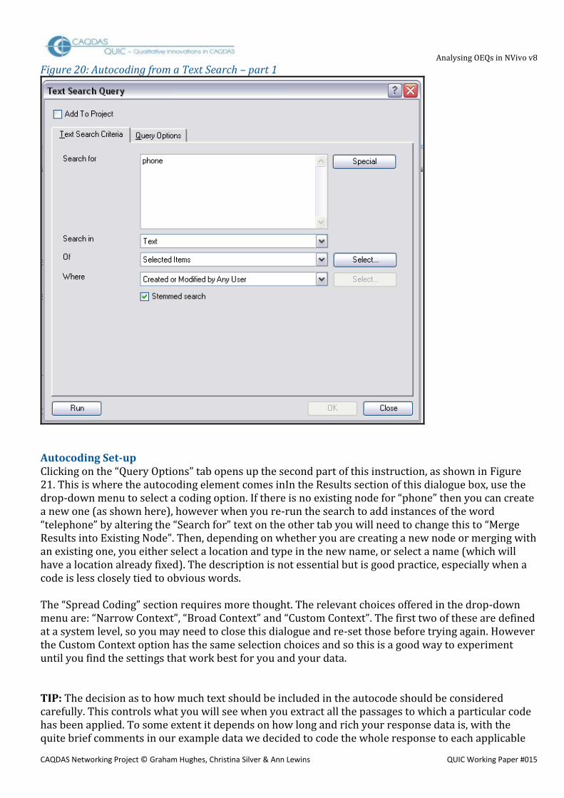
Text Searching Tools Although most qualitative analysts will naturally prefer to do all coding work manually it is quite reasonable in some circumstances to use NVivo’s autocoding process. For example quite a lot of responses may be simply “don’t know” because the open-question has not triggered a specific response. Coding such material individually would be tedious work but by running a Text Search Query (probably first with and then without the apostrophe) and using the Query Options functions these can be allocated to a node quickly and efficiently. With practice more positive common concepts may be identified and also rapidly coded in this way. It should be easier to follow this procedure and then eliminate any incorrect codings, following a consistency check, than to code a large number of very similar statements manually. This is initially started using the drop-down beside “New” on the main toolbar and selecting “New - Text Search Query”. Figure 20 shows the first stage of creating such a query, the same example word “phone” has been used here as the text to search for. Once again the search is limited to Text (ie excluding annotations), but in this option it is necessary to specify which document is to be searched (unlike the Find option which is automatically restricted to the open one). TIP: Note in Figure 8 how the “Stemmed search” box has been ticked, unfortunately this is not as flexible as the Find option so whilst “phones” will probably be found with this instruction, “telephone” will not be found. It is possible to combine multiple words in the search expression, this will be discussed below but, for the moment, we will keep to a simple term in order to establish the procedure clearly.
Analysing OEQs in NVivo v8
CAQDAS Networking Project © Graham Hughes, Christina Silver & Ann Lewins QUIC Working Paper #015
Figure 20: Autocoding from a Text Search – part 1
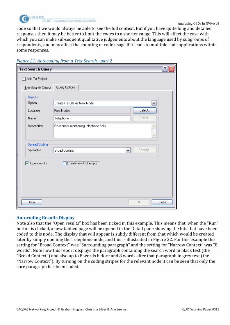
Autocoding Set-up Clicking on the “Query Options” tab opens up the second part of this instruction, as shown in Figure 21. This is where the autocoding element comes inIn the Results section of this dialogue box, use the drop-down menu to select a coding option. If there is no existing node for “phone” then you can create a new one (as shown here), however when you re-run the search to add instances of the word “telephone” by altering the “Search for” text on the other tab you will need to change this to “Merge Results into Existing Node”. Then, depending on whether you are creating a new node or merging with an existing one, you either select a location and type in the new name, or select a name (which will have a location already fixed). The description is not essential but is good practice, especially when a code is less closely tied to obvious words. The “Spread Coding” section requires more thought. The relevant choices offered in the drop-down menu are: “Narrow Context”, “Broad Context” and “Custom Context”. The first two of these are defined at a system level, so you may need to close this dialogue and re-set those before trying again. However the Custom Context option has the same selection choices and so this is a good way to experiment until you find the settings that work best for you and your data. TIP: The decision as to how much text should be included in the autocode should be considered carefully. This controls what you will see when you extract all the passages to which a particular code has been applied. To some extent it depends on how long and rich your response data is, with the quite brief comments in our example data we decided to code the whole response to each applicable
Analysing OEQs in NVivo v8
CAQDAS Networking Project © Graham Hughes, Christina Silver & Ann Lewins QUIC Working Paper #015
code so that we would always be able to see the full context. But if you have quite long and detailed responses then it may be better to limit the codes to a shorter range. This will affect the ease with which you can make subsequent qualitative judgements about the language used by subgroups of respondents, and may affect the counting of code usage if it leads to multiple code applications within some responses.
Figure 21: Autocoding from a Text Search - part 2
Autocoding Results Display Note also that the “Open results” box has been ticked in this example. This means that, when the “Run” button is clicked, a new tabbed page will be opened in the Detail pane showing the hits that have been coded to this node. The display that will appear is subtly different from that which would be created later by simply opening the Telephone node, and this is illustrated in Figure 22. For this example the setting for “Broad Context” was “Surrounding paragraph” and the setting for “Narrow Context” was “8 words”. Note how this report displays the paragraph containing the search word in black text (the “Broad Context”) and also up to 8 words before and 8 words after that paragraph in grey text (the “Narrow Context”). By turning on the coding stripes for the relevant node it can be seen that only the core paragraph has been coded.

Analysing OEQs in NVivo v8
CAQDAS Networking Project © Graham Hughes, Christina Silver & Ann Lewins QUIC Working Paper #015
Figure 22: Results following an Autocoding Query
An important point to note here is that the IDs for the responses have not been included in the coded text. In this display, run as part of the autocoding query, although it is possible to see those IDs because they are in the narrow context extensions, when a Code listing for this node is generated from the Nodes folder it will only show the text that has been coded. This represents a disadvantage arising from using this method to code responses as it may make it more difficult to locate a specific response at a later stage, for example to relate it to the respondent’s socio-demographic attributes. TIP: We have observed that displaying a node by clicking on its name in the List pane during the same working session as that in which the node was created by autocoding will bring up the extended contexts again, but when the project has been saved and closed then subsequent views of that node will only show the coded text. However, you can then open the source document by clicking on the “Text” tab at the right-hand side of the detailed view pane and then double-clicking on the appropriate document icon that will appear in the upper portion of that pane. That document will open in full in a new tab with the relevant coded passages highlighted in it. Before moving on you should now check the accuracy of the coding just carried out. Read each coded text in the Results display carefully to satisfy yourself that they have been correctly coded. If a text is found to have been coded incorrectly this can be adjusted by highlighting it and clicking on the “uncode” button on the Coding toolbar.

Analysing OEQs in NVivo v8
CAQDAS Networking Project © Graham Hughes, Christina Silver & Ann Lewins QUIC Working Paper #015
Advanced Searching It is unlikely that a single search will exhaust the potential autocoding for one code, and the process can be repeated with variations on the search theme, or multiple terms can be used within a single search and autocode procedure. To continue this example we searched for “telephone” which coded a further four responses, other potentially relevant words to try might be “ring” and “call”, although these may generate some incorrect codings as in “ring the church bell” or “call at the door”. Ideas for further text searches may be found from the word frequency tables suggested earlier, and those tables should also indicate the variations in spelling which should be included in the searches. Several words and variations of spelling can be included in one search by using the “Special” button on the Text Search Criteria tab shown above in Figure 20. Different words which have equivalent meanings, such as “loudspeaker” and “loudhailer” can be combined with the “OR” operator, and the usual wildcard characters are also available. Care may be necessary to reduce incorrect hits, for example whilst “*phone” will find ‘telephone’ it will also find ‘microphone’ which is probably not an equivalent term in this data. TIP: NVivo is a little unhelpful when a series of searches is used with a single node because, after each subsequent search and autocode, the full list of references for that node are displayed, and so it becomes increasingly difficult to identify the new additions from the latest run. If this is a significant problem it may be worth considering creating a new node for each search and then, when they have been checked for accuracy and relevance, merging all these similar nodes into a single node. The autocoding process will not complete the task if data reduction to accurate quantities of references is the goal of the analysis (see section 4 below), because of the variety of ways in which many ideas can be expressed. But some time can undoubtedly be saved through the use of well-directed search and autocoding routines.
2.4 Coding – data indexing versus data reduction.
The actual techniques of manually applying codes to segments of text are not discussed here. They are common to all applications of the program and are clearly explained in NVivo’s help manual and in other sources. However, the possible uses to which the analysis of responses to open-ended survey questions may be put is a matter worth discussing further. As a coding scheme is developed and applied to textual data, the analyst will inevitably encounter uncertainty and doubt. Does the text in front of me represent something different from others I have read before which mentioned a particular keyword? A common solution to this is to be generous and inclusive, applying specific codes to a range of comments that initially appear to be connected to those concepts, with the good intention of returning later and checking the work. This activity may be described as “data indexing” as it facilitates the retrieval of various passages that appear to relate to a particular topic. When open-ended questions have been asked in survey situations it may be appropriate to generate numerical summaries of the data, probably in the form of statements of the type “X% of responses to this question mentioned Y”. The obvious source of the numbers for this output is the coding of concept “Y”. However the statement will only be valid if the use of that concept in every one of the responses allocated that code is consistent and equivalent, because the code that is used in this way has effectively replaced the words recorded for each respondent. The original textual data has been reduced to the code label.

Analysing OEQs in NVivo v8
CAQDAS Networking Project © Graham Hughes, Christina Silver & Ann Lewins QUIC Working Paper #015
When put this way it should be apparent that work needs to be done by the analyst to refine the inclusive indexing codes before they can be safely used as summarising reducing codes. In this example data one respondent said “I liked the automated calls” but another commented “The recorded message isn’t very effective”. Initial index coding may have allocated a code “Automated Messages” to both of these passages but it would be potentially misleading to include both in the percentage of respondents who preferred an automated telephone warning system.
2.5 Checking summarising codes – consistency and omissions.
There are a variety of tools in NVivo to assist with the refinement of codes when they have to be reduced to summarise what was originally said. Two particular aspects should be considered, firstly confirmation that all of the passages connected to any one code are all sufficiently similar to be treated as equivalent, and secondly confirmation that no other passages that are also equivalent have been omitted from that code. The first step in confirming consistency or equivalence is to extract all of the passages that have been allocated to a code and read them carefully looking for differences of meaning that might justify exclusion from that group. Extra care may be needed if the code has been used with responses to more than one question. If a code has only been used with a single question then its references can be viewed easily by clicking on that node in the List pane for the Nodes section. This command will open the detailed display of references in the Detail pane where they can be scrolled backwards and forwards to read and compare. If a hard copy is preferred it can be generated by selecting the print command whilst this output is open in the Detail pane.
However, if one node has been used to code the responses to two or more questions then it may be advisable to use a Coding Query to generate a targeted output for consideration. From the New drop-down menu select New Coding Query. The simple tab should provide sufficient criteria for this task. Select the relevant Node in the top part of this dialogue and the Source that holds the responses to the relevant question further down the screen. When the Run command is triggered the Detail pane will display the references for that combination of Node and Source. Again this can be printed by selecting the print command. After checking all of the passages linked to a single code it should be possible to write a concise definition of that code. In NVivo this can be typed into the properties box for that Node. In the List pane for the Nodes section, right-click on the relevant Node name and select Free Node Properties (or Tree Node Properties if applicable), then type the definition into the Description field. If you find it difficult to write a concise definition of a code then it may be inferred that you should not refer to the number of references to that code in any data reducing statements.
It is more difficult to search for code omissions, these are passages which are closely equivalent to those already allocated to a particular code but which have not yet been allocated themselves. One possible method for doing this is to filter-out all of the segments which have been allocated the code and then carry out a series of text searches using key words connected to that code on the remaining text passages. In NVivo this can be done by using a Compound Query, see an illustration in Figure 23.

Analysing OEQs in NVivo v8
CAQDAS Networking Project © Graham Hughes, Christina Silver & Ann Lewins QUIC Working Paper #015
Figure 23: Compound Query to find coding omissions
Using the New drop-down menu select a New Compound Query, as shown in Figure 23 above. The first subquery should be a text search where the Criteria button is used to enter possible key words associated with the relevant code. The second subquery should be a coding query, set to the relevant code. And these two should be linked by the “AND NOT” option. Thus this compound query asks for content containing the specified text in passages that have not been coded to the specified code. Finally it will probably be necessary to limit the query to the relevant source document by selecting that at the “In” field. On the Query Options tab it is useful to set the spread to “Broad context” to help consider the meaning of any positive results. It would be useful to tick the box to add this query to the project because it will need to be run multiple times with variations of the text to be searched on, and that would be easier to edit without having to reset all the other criteria for each run. For this sort of query an empty result represents a success, because it means that the search text has not been found in any relevant passages that have not been coded. Any positive results will need to be investigated carefully as they potentially represent omitted references to that code. Clearly, if the original coding was done by using text searches and autocoding routines as described in section 3 above, there will be little point in repeating those queries at this stage as a check. However, if the main coding work was done manually, that is to say by reading the responses and selecting appropriate codes by hand, then this automated checking procedure should provide a worthwhile check on the accuracy of those human decision processes. In this latter situation the Word Frequency Count information illustrated in Section 2 above may provide useful clues for the texts to be used as criteria in the compound query.

Analysing OEQs in NVivo v8
CAQDAS Networking Project © Graham Hughes, Christina Silver & Ann Lewins QUIC Working Paper #015
Each of these processes may seem to involve a lot of work, so judgement will be necessary to decide how much is appropriate. These checks are important if you are going to use the code frequencies in any statistical analysis or reporting, they are not so significant if you are merely indexing the ideas in your data. If you started with a clear coding scheme and precise definitions of the codes before you began interpreting the texts then you may be more confident that you have applied the codes consistently and accurately. However, if you have worked more inductively, gradually refining the meanings and uses of the codes with ideas found within the texts, then you are more likely to have inconsistencies between the coding you did on earlier readings and those you did later. It is also important to check for these types of error if more than one person has been involved in coding any particular set of texts.
2.6 Looking for similarities or differences?
When analysing the responses to open ended survey questions it may well be easy to slip into the expectation that the most frequently used codes, or rather the concepts to which they refer, are the most important. After all, these are the items that seem to have the most interpretive and statistical ‘weight’. However, it should always be worth looking out for contributions which are different from the common ideas. One-off comments will never feature in the quantitative tables because, by definition, they lack numerical support. But a small number of individuals may well take the opportunity of an open-ended question to add an unexpected thought and these contributions represent a challenge and an opportunity for the analyst. It is worth considering what the purpose behind the inclusion of an open ended question in the survey was. In many situations previous research will have revealed the most likely answers and these will have been included as response categories in closed questions asked elsewhere in the survey, but then an open question has been included to pick up other ideas. In these situations it is the unusual answers which may be of most interest. It is for this reason that it is worth analysing the open-ended questions systematically. For instance, in the data used as an example for these instructions the question QBETT2 was used to ask people what better ways they could think of to warn people when a flood is likely to happen. It may be interesting to note that, out of 229 responses to this question, just four mentioned the problem of previous warnings that had not been followed by actual flooding leading to the important warning being ignored, the so-called “crying wolf” scenario. Maybe more people had this experience but not everybody is brave enough to admit that they ignored a valid warning. Many more people said that they would like to have had an earlier warning and more time to prepare for the flood, but if this obvious response is acted on then it seems likely that there will be more false alarms and a danger that the whole warning system falls into disrepute. It seems that the value of a detailed qualitative analysis of the responses to such a question is an opportunity to pick up the unexpected ideas which would be so easily overlooked in a statistical analysis. Such uncommon ideas may be found by checking the codes which have low frequencies, or by creating an extra code during a manual coding process specifically to identify them – maybe named “Unusual” or even “Z Unusual” to anchor it at the bottom of the coding list. Conclusions: There are many lengthy step-by-step instructions in the above materials. These have been included to help those who are not familiar with certain aspects of the way NVivo works. However this is not intended to imply that these are the correct/only/best ways of analysing the responses to open-ended survey questions in NVivo. These are merely examples of procedures that do work, particularly with

Analysing OEQs in NVivo v8
CAQDAS Networking Project © Graham Hughes, Christina Silver & Ann Lewins QUIC Working Paper #015
data of the sort shown in the examples. However it will always be the case that different data may require different procedures, but we hope that these examples will help some analysts to get over the problem of using unfamiliar software or of using familiar software in an unfamiliar way.
3.0 Quantitative Analysis Strategies for analysing Open-ended Survey Questions in NVivo (v8) In common with other pages in this section of the website, this page is a series of observations about how the features of NVivo might interact with a particular sort of dataset. This page should be read in the context of the related materials concerning the use of NVivo with Open-ended Survey Questions, in particular the Data Preparation Instructions and the Qualitative Analysis Strategies, since the quantitative strategies outlined below can only be effected after the data have been imported and coded systematically in a NVivo project. The tools discussed below are illustrated with examples from the same post flooding event survey that was used to illustrate the data preparation processes. For a summary of the project from which this data derives see here. This data is characterised by a fairly large number of short statements.
Outline: 3.1 Summary of codes applied to a single question 3.2 Matrix Coding Query for summary of codes to several questions 3.3 Matrix Coding Query for analysis of themes with personal attributes 3.4 Matrix Coding Query for analysis of co-occurring thematic codes 3.5 Exporting and Storing Query Results tables 3.6 Summary conclusion
Detailed Guidance:
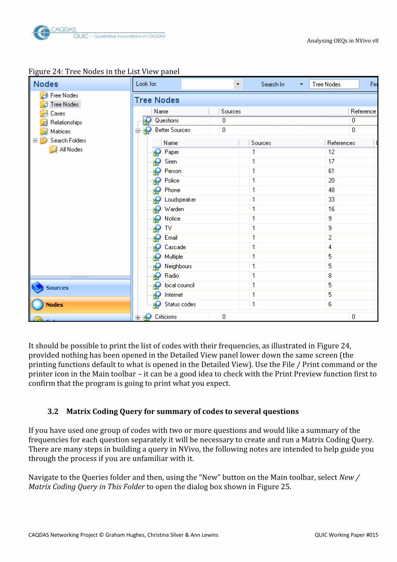
3.1 Summary of codes applied to a single question In many situations the most important output required from the analysis of some open-ended survey question responses will be a simple summary of the number of times each thematic code has been applied to the set of responses to a single question. If you have used a hierarchical structure of coding with a separate group for the set of codes applied to each question, then it should be possible to read off the frequencies in the Nodes List View panel as the simplest way to access this information. In Figure 24, below, a portion of the NVivo working screen is shown with the Nodes navigation panel open and the Tree Nodes in the List View panel. The node group called “Better Sources” has been expanded, and beside each code name it can be seen that it has been used with just a single source and the value in the column headed “References” represents the frequency with which that code has been applied within that source. For example in Figure 24 it can be seen that the code “Siren” has 17 references. Provided the same code has not been used more than once within a single response text, this represents the number of cases that mentioned that theme.
Analysing OEQs in NVivo v8
CAQDAS Networking Project © Graham Hughes, Christina Silver & Ann Lewins QUIC Working Paper #015
Figure 24: Tree Nodes in the List View panel
It should be possible to print the list of codes with their frequencies, as illustrated in Figure 24, provided nothing has been opened in the Detailed View panel lower down the same screen (the printing functions default to what is opened in the Detailed View). Use the File / Print command or the printer icon in the Main toolbar – it can be a good idea to check with the Print Preview function first to confirm that the program is going to print what you expect.
3.2 Matrix Coding Query for summary of codes to several questions If you have used one group of codes with two or more questions and would like a summary of the frequencies for each question separately it will be necessary to create and run a Matrix Coding Query. There are many steps in building a query in NVivo, the following notes are intended to help guide you through the process if you are unfamiliar with it. Navigate to the Queries folder and then, using the “New” button on the Main toolbar, select New / Matrix Coding Query in This Folder to open the dialog box shown in Figure 25.

Analysing OEQs in NVivo v8
CAQDAS Networking Project © Graham Hughes, Christina Silver & Ann Lewins QUIC Working Paper #015
Figure 25: Matrix Coding Query – initial dialog box
This can be a confusing dialog box to complete so take a moment to familiarize yourself with its various components. Note that there are three tabbed pages (Rows / Columns / Matrix) nested within two other pages (Matrix Coding Criteria / Query Options). Note also the small check box in the top left hand corner, “Add To Project”, it is necessary to tick this box in order to save the query for re-use because, if you click on any of the buttons at the bottom of the dialog (Run / OK / Close) without having ticked this, then all of the settings you have created will be wiped away – this can be very frustrating! TIP: We suggest that you tick the “Add To Project” box at an early stage and give the query a name, then if it doesn’t generate the output that you want you can come back and edit it until it does work correctly. As soon as you click on this box a third tabbed page is added to the dialog box called “General” with an obvious field to enter the query’s name. In this example we used “QBETT2 Better Sources” as the name, to indicate that this query works with the set of codes for “better sources” and the question document for QBETT2. This also brings the “OK” button into use, although it is not worth

Analysing OEQs in NVivo v8
CAQDAS Networking Project © Graham Hughes, Christina Silver & Ann Lewins QUIC Working Paper #015
pressing it yet as this just saves the current version of the query and closes the dialog box without running the query or generating any results. Having given the query a name, it is best to work on the Matrix Coding Criteria tab next. For the type of table we are trying to generate in this example the rows of the table will be formed of thematic codes from the Nodes section and the columns will be question documents from the Sources section of the data. To define the rows, first click on the Rows tab (if it is not already open) and then click on the “Select” button within that tab area. This opens another dialog box similar to that shown in Figure 26, below. Figure 26: Select Items dialog box within Matrix Coding Query
The illustration in Figure 26 has been taken part way through the selection process. Here, we have already navigated to the Tree Nodes section by clicking on its selection box in the left hand panel, then we expanded the “Better Sources” group of codes by clicking on the “+” box to the left of its check box to display the full list of codes in that group. By clicking on the “Automatically select hierarchy” check box at the top of this dialog, it is possible to select all of that group of codes by just clicking on the check box beside the group header, and this has inserted ticks beside all of the codes in that group. It is possible to continue selecting more codes and code groups if necessary until all the requirements for the rows of the output table have been fulfilled. Finish this dialog by clicking on the “OK” button to return to the Matrix Coding Query dialog box. TIP: There is a tempting “Select All” button in Figure 26, but if you click on this it will literally select everything in the project which will be much more than you need. So we recommend that you select the code groups that you need one at a time. When you click on the “OK” button at the end of the selection process in Figure 26 you will be returned to the dialog shown in Figure 25, which will not show any apparent change. It is important that you now click on the “Add to List” button (which was greyed-out before but is now usable) – because this

Analysing OEQs in NVivo v8
CAQDAS Networking Project © Graham Hughes, Christina Silver & Ann Lewins QUIC Working Paper #015
is needed to insert the selected codes into the query. Only after this has been done do you see the beginning of the list of codes in the Rows tab of the query, see Figure 27 below for an illustration. Figure 27: Matrix Coding Query after defining rows
A click on the Columns tab moves the dialog to the page for defining those elements of the table. This is done in a similar way to the rows. Click on the Select button to open the Select Project Items dialog box once more. This time navigate to the Sources area and select one or more question documents as required for your output. In this example we have selected three question documents (“QMORE”, “QBETT2”, & “QADVI2”), closed that dialog with “OK”, then clicked on “Add to List” on the Columns tabbed page to get to the stage shown in Figure 28 below.

Analysing OEQs in NVivo v8
CAQDAS Networking Project © Graham Hughes, Christina Silver & Ann Lewins QUIC Working Paper #015
Figure 28: Selecting the columns in a Matrix Coding Query
Note that for this particular query it will not be necessary to use the section near the bottom of the dialog box which shows “In – All Sources”. This part of the query can be used to limit the number of documents searched, it is not necessary because we have defined the sources to be used as the columns of the matrix already. In other types of query this section may be more significant. The Matrix tab does not need altering for this query as the default setting of “AND” is what is needed to generate the required output. The Query Options tab should also default to the appropriate setting of “Preview Only” as this will send the output table to the screen in the Detailed View panel. It is now worth pressing the “OK” button to save the query settings. It will then be necessary to reopen the query from the list in order to run it. Alternatively, pressing “Run” when the “Add to Project” box has been ticked will save the query settings and generate the output. The output table from this query is shown in Figure 29, below. Normally this table would be shown in the Detailed View panel but for this screenshot it has been undocked (using the View menu option) so that it appears in a separate window. It is important that the “Grid” toolbar is open in either display (docked or undocked) because you will need to use the pull down menu in that toolbar to select “Cases

Analysing OEQs in NVivo v8
CAQDAS Networking Project © Graham Hughes, Christina Silver & Ann Lewins QUIC Working Paper #015
Coded” as shown here. The default setting of “Sources Coded” merely displays “1” in each cell where there is any coding for the question. TIP: all of the settings accessible from the “Grid” toolbar are also available through a right-click context menu when the mouse pointer is anywhere in the table. Figure 29: Output Table from Matrix Coding Query for coding frequencies by question
As can be seen in Figure 29, the set of codes selected for this query have not been used with the questions labeled “QMORE” and “QADVI2”. This is confirmation that the frequencies taken from the List view panel in Figure 24 were correctly attributed to the QBETT2 question. This table can be printed by using the Print Preview or Printer icons on the Main toolbar within its own window. If it has not been undocked, those same icons in the Main toolbar of the full window will apply to the open item in the Detailed View panel. More advice on exporting and saving output tables is given in Section 5 below.

Analysing OEQs in NVivo v8
CAQDAS Networking Project © Graham Hughes, Christina Silver & Ann Lewins QUIC Working Paper #015
3.3 Matrix Coding Query for analysis of themes with personal attributes
The same basic routine of the Matrix Coding Query can be used for a variety of analytical purposes. When personal attributes, such as age, gender or employment status have been recorded in the NVivo Casebook they can be combined with thematic codes to explore quantitative patterns in the responses that may be influenced by those attributes. A suggested layout for such an analysis would be to have the thematic codes again set up in the rows of the table, while the columns contain the range of values for a single attribute parameter. To use the attribute parameter in this way it is necessary to include them in the column settings of the query. Repeat the steps as before up to Figure 27, and then click on the Columns tab and use the Select button to open the “Select Project Items” dialog once more. This time select the “Attributes” section in the left margin to display the list of attribute variables in the main area. You can expand any of the attributes to show the list of values it can take by clicking on the “+” box beside it. This is shown in Figure 30, below, where the attribute “tenure” has been expanded and all of the positive values it can take have been selected. When the “OK” button is clicked all of the ticked values are made available to the main query, but you have to click on the “Add to List” button to insert them into the query. Figure 30: Selecting Attribute values in a Matrix Coding Query
For this query it is probably also necessary to limit the calculations to the single question for which we want the analysis. This is done at the bottom of the query dialog box, in the area showing “In … Selected Items” by using the “Select” button to open the “Select Project Items” dialog once more and this time using the “Internals” section on the left to navigate to the question Source documents and clicking beside the required question document, followed by “OK”. In Figure 31, below, we show the result of this query where the same thematic codes for Better Sources of warnings have been taken from the source question document QBETT2, analysed against the length of time respondents had lived in the home where they were interviewed (the variable called “tenure”). In this table the length of tenure increases as one reads further to the right.
Analysing OEQs in NVivo v8
CAQDAS Networking Project © Graham Hughes, Christina Silver & Ann Lewins QUIC Working Paper #015
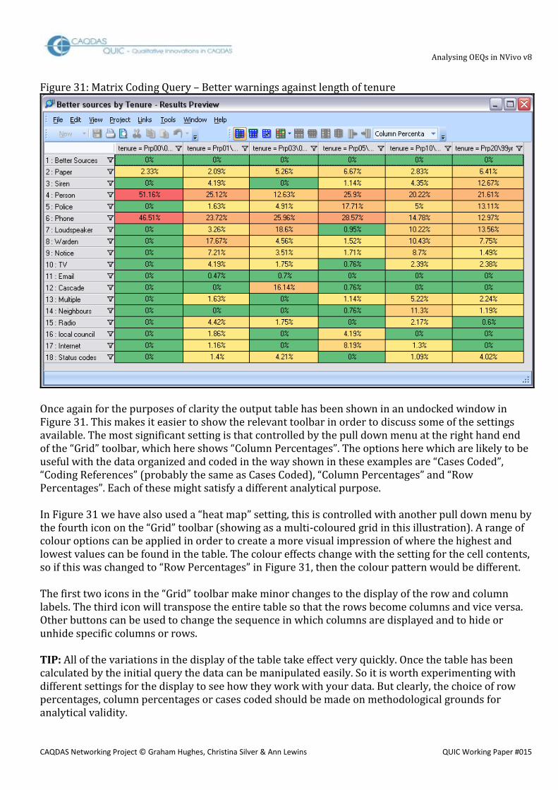
Figure 31: Matrix Coding Query – Better warnings against length of tenure
Once again for the purposes of clarity the output table has been shown in an undocked window in Figure 31. This makes it easier to show the relevant toolbar in order to discuss some of the settings available. The most significant setting is that controlled by the pull down menu at the right hand end of the “Grid” toolbar, which here shows “Column Percentages”. The options here which are likely to be useful with the data organized and coded in the way shown in these examples are “Cases Coded”, “Coding References” (probably the same as Cases Coded), “Column Percentages” and “Row Percentages”. Each of these might satisfy a different analytical purpose. In Figure 31 we have also used a “heat map” setting, this is controlled with another pull down menu by the fourth icon on the “Grid” toolbar (showing as a multi-coloured grid in this illustration). A range of colour options can be applied in order to create a more visual impression of where the highest and lowest values can be found in the table. The colour effects change with the setting for the cell contents, so if this was changed to “Row Percentages” in Figure 31, then the colour pattern would be different. The first two icons in the “Grid” toolbar make minor changes to the display of the row and column labels. The third icon will transpose the entire table so that the rows become columns and vice versa. Other buttons can be used to change the sequence in which columns are displayed and to hide or unhide specific columns or rows. TIP: All of the variations in the display of the table take effect very quickly. Once the table has been calculated by the initial query the data can be manipulated easily. So it is worth experimenting with different settings for the display to see how they work with your data. But clearly, the choice of row percentages, column percentages or cases coded should be made on methodological grounds for analytical validity.

Analysing OEQs in NVivo v8
CAQDAS Networking Project © Graham Hughes, Christina Silver & Ann Lewins QUIC Working Paper #015
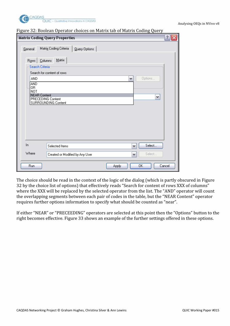
3.4 Matrix Coding Query for analysis of co-occurring thematic codes A third way of using the Matrix Coding Query is to search for possible patterns between co-occurring codes. This may be particularly useful when two or more dimensions in the data have been coded separately. For example in our flooding experience data one dimension was factually based in terms of the specific warning systems mentioned in the response, while the other was more evaluative in assessing the level of criticism identified in the response. After coding has been done in this way it becomes possible to look for patterns to see if certain warning systems were mentioned more often in the negative or critical responses while others were generally referred to in more positive ways. For this type of query one set of thematic codes is listed in the rows of the matrix while another set of thematic codes is listed in the columns. In some situations it may be useful to list the same set of codes in both rows and columns to see where some of them co-occur with others – for example did those who mentioned sirens or loudspeakers also mention the Police? However, this sort of matrix may be particularly affected by the way in which the thematic codes were applied earlier in the project. If you have always applied the thematic codes to the whole of each response (probably by using the custom “paragraph” setting when autocoding following a Text Search Query) then the basic intersection operator “AND” should work well. On the other hand, if you have applied the thematic codes more selectively to only a few words at a time, then the coded sections may not always overlap when two codes have been applied to a single response, and you may have more difficulty getting consistently accurate information about when they co-occur in separate sections of individual responses. Developing this type of query involves listing the appropriate thematic codes in the rows and columns in ways similar to those described above. The difference now is that the third tab in the dialog box for the query, the one labeled “Matrix” may now be more significant. Figure 32 shows the first set of choices to be made with a pull down menu on this tab.
Analysing OEQs in NVivo v8
CAQDAS Networking Project © Graham Hughes, Christina Silver & Ann Lewins QUIC Working Paper #015
Figure 32: Boolean Operator choices on Matrix tab of Matrix Coding Query
The choice should be read in the context of the logic of the dialog (which is partly obscured in Figure 32 by the choice list of options) that effectively reads “Search for content of rows XXX of columns” where the XXX will be replaced by the selected operator from the list. The “AND” operator will count the overlapping segments between each pair of codes in the table, but the “NEAR Content” operator requires further options information to specify what should be counted as “near”. If either “NEAR” or “PRECEEDING” operators are selected at this point then the “Options” button to the right becomes effective. Figure 33 shows an example of the further settings offered in these options.

Analysing OEQs in NVivo v8
CAQDAS Networking Project © Graham Hughes, Christina Silver & Ann Lewins QUIC Working Paper #015
Figure 33: Further Options for some Boolean Operators in Matrix Coding Query
Of these choices it is likely that only the “In Custom Context” will prove useful if your underlying thematic coding has been applied to short segments within the responses from each case. This will allow you to apply yet another dialog box by pressing the “Specify” button which can be seen in Figure 33. Figure 34, below, illustrates the custom context setting dialog box that opens when you select the Specify button in Figure 33. The setting here will determine whether two coded segments will be deemed to co-occur with each other. It is our suggestion that, with data of the sort we are considering here, the “Surrounding paragraph” setting should be appropriate as each response was set up in a separate paragraph in the data preparation stage of this work. If you use the number of words option (and you then have to choose a fixed number to complete that setting) then there will be occasions when you get a false co-occurrence with a coded segment at the end of one response apparently co-occurring with another at the start of the next response.

Analysing OEQs in NVivo v8
CAQDAS Networking Project © Graham Hughes, Christina Silver & Ann Lewins QUIC Working Paper #015
Figure 34: Setting the Custom Context for Proximity Operators
Having chosen a proximity setting and clicked the “OK” box within that dialog box, you will be returned to the Coding Search Operator dialog (as in Figure 33). We would recommend that you tick both of the first two boxes in the “Retrieve” section (“Finds for first search item” and “Finds for second search item”) in order to be given both coded segments in the results. It may also be worth considering the third box in that sections as well, “Content between finds” in order to be given any further text that separated those coded segments – this would be necessary if you have only coded small sections of text within longer responses. Finish that dialog box with its “OK” button to return to the main query dialog box. Make sure that you have specified the source document with the responses to the survey question that you are analyzing, and that you have chosen to add the query to your project (ie to save it) – because after applying so many dialog settings you don’t want to have to re-apply all of them if the query does not quite deliver the expected output.
3.5 Exporting and Storing Query Results tables At the end of section 2, above, we mentioned that it is possible to print the output table from a Matrix Coding Query by clicking somewhere in the table in the Detailed View panel and selecting the menu option File / Print (or File / Print Preview to check what will be printed and then printing from that display). It is also possible to export the table to a spreadsheet in Microsoft Excel format, or to store it within your NVivo Project to re-open it in another working session without having to recalculate.

Analysing OEQs in NVivo v8
CAQDAS Networking Project © Graham Hughes, Christina Silver & Ann Lewins QUIC Working Paper #015
To export an output table to Microsoft Excel, first click inside its window or panel to make it the active object, and then select Project / Export Result from the main menus at the top of the screen. This brings up a standard Windows “Save As” dialog box in which you can select a location and a file name to store the exported table. The only choice of file formats is between a “*.txt” text file or “*.xls” MS Excel file. Storing the results within NVivo is a little more complicated since this has to be specified within the Query itself on the “Query Options” tab. The first field on this part of the dialog is called “Options” and has a pull down menu with two choices: the default “Preview only” and “Create Results as New Matrix”. If you select the latter then you will be asked to select a location and enter a name in a field further down the box. If you have already ticked the box to save the query (the “Add to Project check box) and given the query a name, then that name will be suggested as the default name for the result table. The default location for storing such tables is the “Results” sub-folder in the Queries section of the data. TIP: It is possible to store the results of a query without saving the query itself, by defining a result name on the Query Options tab and not choosing to “Add to Project”. However, this will create a kind of orphaned results file with no means of displaying the parameters under which it was created. So we would recommend saving both the query and its results table under similar names in order to have some means of knowing how those results were generated when you view them at a later date. If you plan to re-run the query after doing more coding or adding more data then it may be useful to include a version number or date of running to the Results table name in order to distinguish those run on different occasions.
3.6 Summary conclusion Many qualitative analysts, who would be familiar with these CAQDAS programs, may be reluctant to use quantifying statements about the data that they analyse. This would be for the very good reason that most often the size of the sample that they are working with is too small to justify a numerical conclusion. However, when one is working with survey data then there is more likelihood that the sample size is sufficiently large and sufficiently random to support some quantified statements. At the same time many quantitative analysts may be wary of applying statistical techniques to data which has been coded separately from the data collection process. However, provided the data collection process was sufficiently robust to capture the data accurately, then the fact that the codes have been applied by research analysts rather than the respondents themselves should not be a reason to water-down the analysis processes. Because the coding process is transparent and replicable, the coded data may be used with more confidence than that derived from the ‘amateur’ coders of the respondents to closed questions. Thus, if quantitative conclusions are being drawn from the rest of the survey data, then there should be no reason why quantitative conclusions cannot be drawn from the open-ended question responses as well.

Analysing OEQs in NVivo v8
CAQDAS Networking Project © Graham Hughes, Christina Silver & Ann Lewins QUIC Working Paper #015
Export Data to Statistical Packages after analysing Open-ended Survey Questions in NVivo (v8) In common with other pages in this section of the website, this page is a series of observations about how the features of NVivo might interact with a particular sort of dataset. This page should be read in the context of the related materials concerning the use of NVivo with Open-ended Survey Questions, in particular the Data Preparation Instructions and the Qualitative Analysis Strategies, since the export strategies outlined below can only be effected after the data have been imported and coded systematically in a NVivo project. The tools discussed below are illustrated with examples from the same post flooding event survey that was used to illustrate the data preparation processes. For a summary of the project from which this data derives see here. This data is characterised by a fairly large number of short statements.
Outline: 4.1 Use of Matrix Coding Query 4.2 Editing in MS Excel 4.3 Checking data transfer
Detailed Guidance:
4.1 Use of Matrix Coding Query In summary the procedure for extracting code frequencies at the level of respondent cases is to create a Matrix Coding Query with a row for each case and a column for each code variable, and to store the results of running that query as a new matrix. That new matrix can then be exported to MS Excel in a readily accessible format. Open a new query by navigating to the Queries folder, clicking on the ”New” button in the main toolbar and selecting New Matrix Coding Query in This Folder from the pull-down menu there. It is probably a good idea to save this query for possible re-use so, before getting into the detailed parameters, click on the “Add to Project” box and give the query a name on the General tab that immediately opens up. Then click on the “Matrix Coding Criteria” tab which has three tabbed sub-pages “Rows”, “Columns” and “Matrix”. Working initially on the “Rows” page, click on the “Select” button in the “Define More Rows” section to open the “Select Project Items” dialog window.
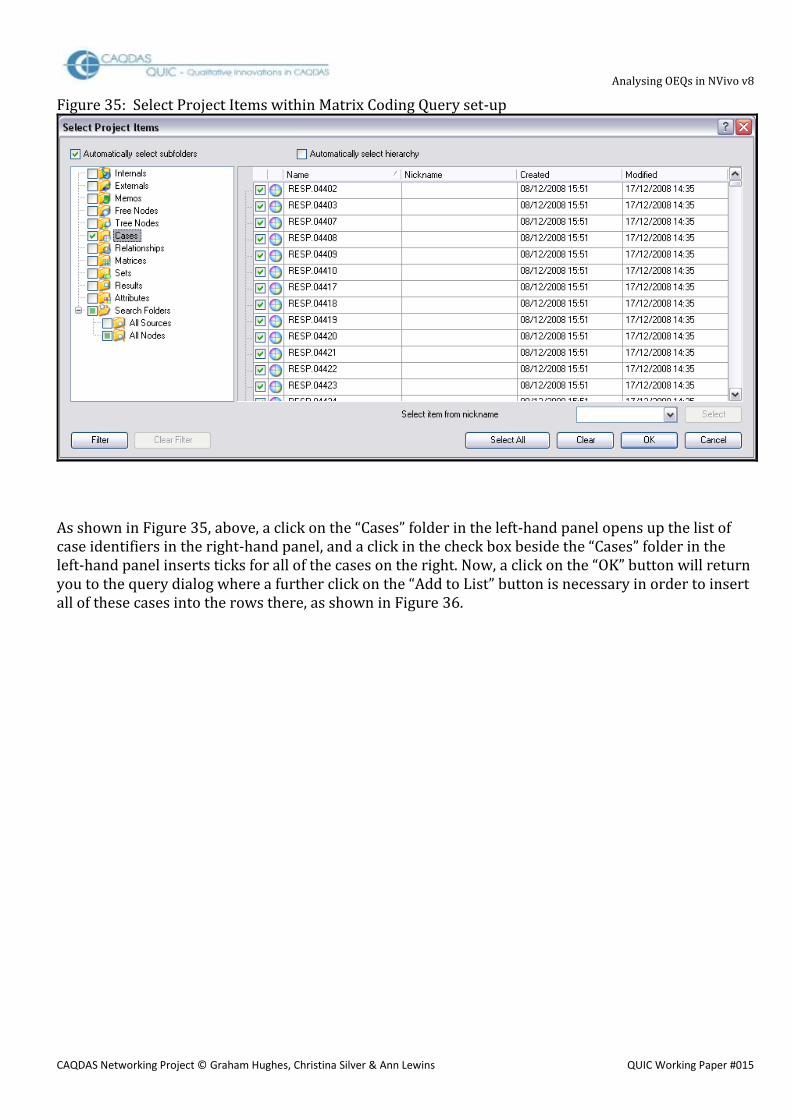
Analysing OEQs in NVivo v8
CAQDAS Networking Project © Graham Hughes, Christina Silver & Ann Lewins QUIC Working Paper #015
Figure 35: Select Project Items within Matrix Coding Query set-up
As shown in Figure 35, above, a click on the “Cases” folder in the left-hand panel opens up the list of case identifiers in the right-hand panel, and a click in the check box beside the “Cases” folder in the left-hand panel inserts ticks for all of the cases on the right. Now, a click on the “OK” button will return you to the query dialog where a further click on the “Add to List” button is necessary in order to insert all of these cases into the rows there, as shown in Figure 36.

Analysing OEQs in NVivo v8
CAQDAS Networking Project © Graham Hughes, Christina Silver & Ann Lewins QUIC Working Paper #015
Figure 36: Matrix Coding Query – Case identifiers in rows
Next, click on the “Columns” tab to define the other dimension of the table. The centre of the dialog will be blank until you have selected the appropriate codes and added them to the query. As with the rows tab, click on the “Select” button in the section “Define More Columns” to open the “Select Project Items” dialog once more. This time, as shown in Figure 37 below, click on the “Tree Nodes” (or “Free Nodes” if that is where the relevant codes are listed) in the left-hand panel to view lists of codes in the right-hand panel. If you have grouped codes in hierarchical structures you may need to expand these by clicking on the “+” boxes beside the group headers to see the full lists.

Analysing OEQs in NVivo v8
CAQDAS Networking Project © Graham Hughes, Christina Silver & Ann Lewins QUIC Working Paper #015
Figure 37: Selecting Codes for frequencies output
Here, we have expanded the group “Better Sources” and then selected all of its members by clicking on the check box above the lists “Automatically select hierarchy” and then the check box beside “Better Sources”. If you wish to exclude some codes from the export from within the group, a further click on the check box beside those items will untick them. Alternatively, you may prefer to select specific codes for the export by ticking them directly one at a time. As with the cases before, when you are satisfied with your selections click on the “OK” button in this dialog box and then the “Add to List” button in the query dialog box. This should bring you to a view similar to Figure 38.
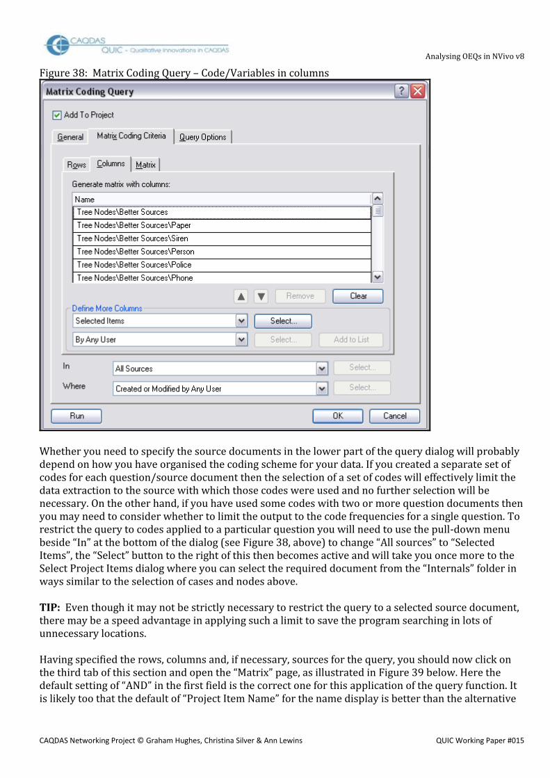
Analysing OEQs in NVivo v8
CAQDAS Networking Project © Graham Hughes, Christina Silver & Ann Lewins QUIC Working Paper #015
Figure 38: Matrix Coding Query – Code/Variables in columns
Whether you need to specify the source documents in the lower part of the query dialog will probably depend on how you have organised the coding scheme for your data. If you created a separate set of codes for each question/source document then the selection of a set of codes will effectively limit the data extraction to the source with which those codes were used and no further selection will be necessary. On the other hand, if you have used some codes with two or more question documents then you may need to consider whether to limit the output to the code frequencies for a single question. To restrict the query to codes applied to a particular question you will need to use the pull-down menu beside “In” at the bottom of the dialog (see Figure 38, above) to change “All sources” to “Selected Items”, the “Select” button to the right of this then becomes active and will take you once more to the Select Project Items dialog where you can select the required document from the “Internals” folder in ways similar to the selection of cases and nodes above. TIP: Even though it may not be strictly necessary to restrict the query to a selected source document, there may be a speed advantage in applying such a limit to save the program searching in lots of unnecessary locations. Having specified the rows, columns and, if necessary, sources for the query, you should now click on the third tab of this section and open the “Matrix” page, as illustrated in Figure 39 below. Here the default setting of “AND” in the first field is the correct one for this application of the query function. It is likely too that the default of “Project Item Name” for the name display is better than the alternative

Analysing OEQs in NVivo v8
CAQDAS Networking Project © Graham Hughes, Christina Silver & Ann Lewins QUIC Working Paper #015
“Hierarchical Name” in order to get more usable variable names as the column headers in the output table. Figure 39: Settings for the Matrix page
Finally, having completed the specification for the contents of the output, you need to click on the “Query Options” tab in order to direct the output to a Results table which can be exported to MS Excel. This page is shown in Figure 40, below. It is probably advisable to set the first field on this page to “Create Results as New Matrix” (as shown here) rather than the default “Preview” in order to get the table stored in the Results section of your project where it can be accessed again much more quickly than by re-running the query. Setting the Option in this way activates the “Select” button for the “Location” field and the “Name” field for finding the results table again in the future.

Analysing OEQs in NVivo v8
CAQDAS Networking Project © Graham Hughes, Christina Silver & Ann Lewins QUIC Working Paper #015
Figure 40: Query Options page settings
As can be seen in Figure 40, there are two check boxes in this dialog but these only become active when the “Results” option is changed to “Create Results as New Matrix”. The first of these, “Open results”, simply makes the program open the display of the output table in the Detailed View panel when the search and calculations are complete. The second, “Create results if empty” appears to refer to the entire query and not to individual data lines thus, as long as there is at least one code reference in the set of codes and sources that you have defined on the Matrix Coding Criteria pages, you will get a full table listing every case and code that you have defined whether you tick this box or not. In our example data we have tried running the same query with this box ticked and unticked and on both occasions obtained a matrix with 1,257 rows, even though some of them had zero for every variable. Finally, you can press the “Run” button to set the query running. This will save the query in the “Queries” folder with the name you gave it on the “General” tab, store the output table in the “Results” folder with the name you gave it on the “Query Options” tab, and display the table in the Detailed View panel (if you ticked the “Open results” box). The “Apply” and “OK” buttons will simply save the query without running it. A portion of the output table obtained from this query is shown in Figure 41, below.
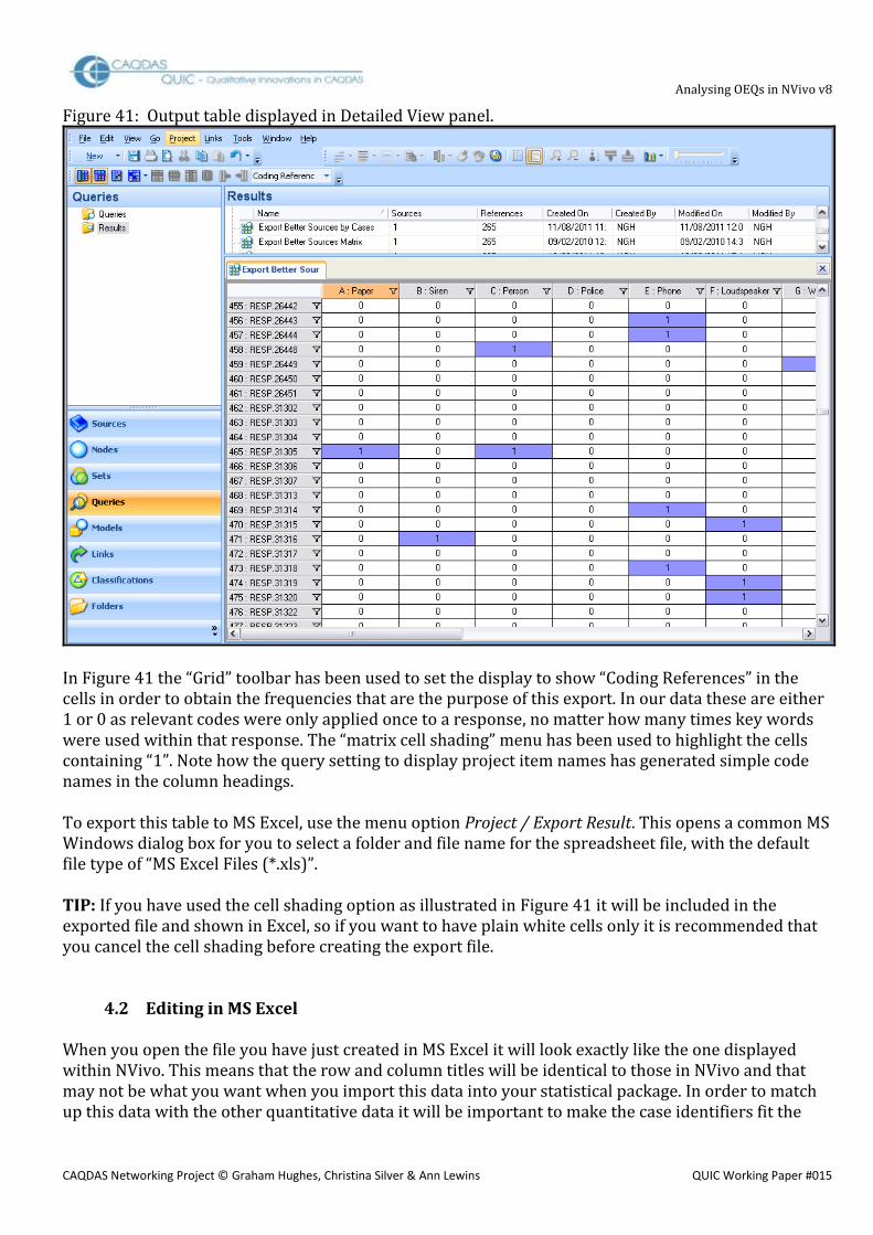
Analysing OEQs in NVivo v8
CAQDAS Networking Project © Graham Hughes, Christina Silver & Ann Lewins QUIC Working Paper #015
Figure 41: Output table displayed in Detailed View panel.
In Figure 41 the “Grid” toolbar has been used to set the display to show “Coding References” in the cells in order to obtain the frequencies that are the purpose of this export. In our data these are either 1 or 0 as relevant codes were only applied once to a response, no matter how many times key words were used within that response. The “matrix cell shading” menu has been used to highlight the cells containing “1”. Note how the query setting to display project item names has generated simple code names in the column headings. To export this table to MS Excel, use the menu option Project / Export Result. This opens a common MS Windows dialog box for you to select a folder and file name for the spreadsheet file, with the default file type of “MS Excel Files (*.xls)”. TIP: If you have used the cell shading option as illustrated in Figure 41 it will be included in the exported file and shown in Excel, so if you want to have plain white cells only it is recommended that you cancel the cell shading before creating the export file.
4.2 Editing in MS Excel When you open the file you have just created in MS Excel it will look exactly like the one displayed within NVivo. This means that the row and column titles will be identical to those in NVivo and that may not be what you want when you import this data into your statistical package. In order to match up this data with the other quantitative data it will be important to make the case identifiers fit the

Analysing OEQs in NVivo v8
CAQDAS Networking Project © Graham Hughes, Christina Silver & Ann Lewins QUIC Working Paper #015
format of their equivalents in the statistics package, and you will want to have variable names that are usable in the statistics package. Thus some editing of the first row and column of the data is likely to be necessary. It is most likely that the case identifiers in the statistics package are simply the numbers at the end of the alpha-numeric strings that have been used in NVivo. These can be extracted with a few procedures outlined below. The first step in cleaning up the case identifiers is to insert two new columns between the current column A and the first column of code data, ie between columns A and B in the workbook. The corrected IDs will be created in these new columns. In our example the required data are the last five digits of the text in column A, and these can be extracted by typing the logic =RIGHT(A2,5) into the cell at B2 (in the new empty column just previously inserted) and then copying that logic all the way down column B. It will then be necessary to convert these logical statements that display the correct digits into absolute values in the new column C. This final step involves copying all of column B and then pasting it into column C with a “paste special” command to store “values” only. When this has been completed and checked for accuracy, columns A and B can be deleted and the workbook can be saved. The column headers in row 1 of the spreadsheet are likely to be used by the statistics package as the names of the new variables whose data is in those columns. Here the problem lies with the prefix letters that NVivo has inserted in front of the code name. On the assumption that the number of variables exported is not very large it is probably simplest to edit these manually as with any text cell in MS Excel. When you are satisfied that the row and column identifiers are in the correct format for importing into the statistics program, save and close the spreadsheet file.
4.3 Checking data transfer Whenever large amounts of data are moved between programs there will be potential sources of error so, before continuing with the analysis in your statistical package, it would be advisable to check a small sample of cases in that package to confirm that the code frequencies have been matched with the correct cases. This is not simply a matter of confirming that the total frequency for each imported code variable is the same in NVivo and your statistical program but also that individual cases have correct codes.