100% renewable electricity in Australia

February 2017

Andrew Blakers, Bin Lu and Matthew Stocks

Australian National University

Andrew.blakers@anu.edu.au | ph 61 2 6125 5905

Abstract We present an energy balance analysis of the Australian National Electricity Market (NEM) in a 100% renewable energy scenario in which wind and photovoltaics (PV) provides 90% of the annual electricity. The key outcome of our modelling is that the additional cost of balancing renewable energy supply with demand on an hourly basis throughout the year is modest: AU$25-30/MWh (US$19-23/MWh).

In our modelling we avoid heroic assumptions about future technology development by only including technology that has already been deployed in large quantities (> 100 Gigawatts), namely PV, wind, high voltage transmission (HVDC, HVAC) and pumped hydro energy storage (PHES). PHES constitutes 97% of worldwide electricity storage but is neglected in many analyses.

In our scenarios wind and PV contributes about 90% of annual electricity, while existing hydroelectricity and biomass contributes about 10%. We use historical data for wind, sun and demand for every hour of the years 2006-10. Very wide distribution of PV and wind reduces supply shortfalls by taking advantage of different weather systems. Energy balance between supply and demand is maintained by adding sufficient PHES, HVDC/HVAC and excess wind and PV capacity. We term the cost of these additions as the levelised cost of balancing (LCOB). LCOB plus the levelised cost of annual generation (LCOG), combine to give the levelised cost of electricity (LCOE).

Using 2016 prices prevailing in Australia, we estimate that LCOB is AU$28/MWh, LCOG is AU$65/MWh and LCOE is AU$93/MWh. This can be compared with the estimated LCOE from a new supercritical black coal power station in Australia of AU$80/MWh. Much of Australia’s coal power stations will need to be replaced over the next 15 years. LCOE of renewables is almost certain to decrease due to rapidly falling cost of wind and PV. With PV and wind in the price range of AU$50/MWh, the LCOE of a balanced 100% renewable electricity system is around AU$75/MWh.

Importantly, the LCOB calculated in this work is an upper bound – we use 2016 prices and do not include demand management or batteries. A large fraction of LCOB relates to periods of several successive days of overcast and windless weather that occur once every few years. Substantial reductions in LCOB are possible through contractual load shedding, the occasional use of legacy coal and gas generators to charge PHES reservoirs, and management of the charging times of batteries in electric cars.

Although we have not modelled dynamical stability on a time scale of sub-seconds to minutes we note that PHES can provide excellent inertial energy, spinning reserve, rapid start, black start capability, voltage regulation and frequency control.

Introduction It is interesting to consider the practicalities of supplying all of Australia’s electricity from renewable energy. In our study we model scenarios in which the National Electricity Market (NEM) is exclusively supplied by renewable energy. We focus on energy balance (meeting demand for every hour of the year).

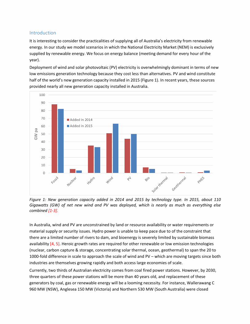
Deployment of wind and solar photovoltaic (PV) electricity is overwhelmingly dominant in terms of new low emissions generation technology because they cost less than alternatives. PV and wind constitute half of the world’s new generation capacity installed in 2015 (Figure 1). In recent years, these sources provided nearly all new generation capacity installed in Australia.

Figure 1: New generation capacity added in 2014 and 2015 by technology type. In 2015, about 110 Gigawatts (GW) of net new wind and PV was deployed, which is nearly as much as everything else combined [1-3].

In Australia, wind and PV are unconstrained by land or resource availability or water requirements or material supply or security issues. Hydro power is unable to keep pace due to of the constraint that there are a limited number of rivers to dam, and bioenergy is severely limited by sustainable biomass availability [4, 5]. Heroic growth rates are required for other renewable or low emission technologies (nuclear, carbon capture & storage, concentrating solar thermal, ocean, geothermal) to span the 20 to 1000-fold difference in scale to approach the scale of wind and PV – which are moving targets since both industries are themselves growing rapidly and both access large economies of scale.

Currently, two thirds of Australian electricity comes from coal fired power stations. However, by 2030, three quarters of these power stations will be more than 40 years old, and replacement of these generators by coal, gas or renewable energy will be a looming necessity. For instance, Wallerawang C 960 MW (NSW), Anglesea 150 MW (Victoria) and Northern 530 MW (South Australia) were closed

during 2013-16, and Hazelwood 1640 MW (Victoria) is set to close in 2017 [6, 7]. It seems unlikely that more coal fired generators will be constructed in Australia due to public opposition and risk aversion of financiers.

Australia has excellent wind and solar resources. If current deployment rates of PV and wind (approximately 1 Gigawatt (GW) per year of each) continue then about half of the electricity generated in Australia in 2030 will come from renewable energy sources. In the state of South Australia wind and PV already provide about half of the annual electricity generation. The nearly zero marginal cost of PV and wind generation means that PV and wind electricity (when available) are used in preference to electricity from coal and gas. This causes declining system capacity factors for coal and gas power stations, which causes economic pressure on their continued operation. However, closure of coal and gas power stations removes the ancillary benefits that they provide, including coping with periods of poor solar and wind availability and managing short term supply fluctuations over differing time periods via inertia, spinning reserve and dispatchability.

This work differs from previous international work that examines high renewable energy futures in a range of countries. Bogdanov and Breyer [8] provide a good summary of previous work. Key differences in previous work compared with ours includes:

• PHES as a primary energy storage mechanism is generally overlooked; PHES constitutes 97% of worldwide storage for the electricity industry;

• Much of the work is based on national analysis of relatively small countries where the weather and demand is similar everywhere, whereas large-scale interconnection (as in this paper) accesses a wide range of different weather and demand profiles.

• Focus is generally on northern countries (Europe, north Asia, north America) for which heating loads are high and there is strong variation of solar energy supply by season. However, most of the world’s population (including most Australians) live in latitudes lower than 35° for which there is low winter heating load and far less seasonality;

• Speculative technologies that have been deployed on only a small scale (<10 GW) are often included, whereas we avoid speculative technologies in our work by only including those with global deployment above 100 GW. Because of mass production, wind and PV are considerably cheaper than alternative low emission technologies (except in special circumstances).

Our estimated cost of supply of 100% renewable electricity is considerably lower than previous estimates, mostly because of the above-mentioned differences.

Modelling assumptions We model the National Electricity Market (NEM) which services 19 million people [9], but exclude the much smaller systems that exist in Western Australia, the Northern Territory and remote regions in other states (which are not connected to the NEM).

In our modelling, we make the following conservative assumptions:

• We assume that NEM demand remains stable at 205 TWh per year. NEM demand has changed little since 2008 [10], with energy efficiency and behind-the-meter PV offsetting growth in

demand in various sectors. We also exclude electrification of land transport (which could add 30-35% to electricity demand in the future) [11].

• We exclude batteries. Batteries located in homes and electric cars may contribute very substantially to future energy storage, either directly through bi-directional energy flow or indirectly through control of the timing of battery charging.

• We avoid heroic assumptions about future technology development: we only consider technology that has already been deployed in large quantities (> 100 GW), namely PV, wind, high voltage DC (HVDC) and AC (HVAC) transmission and pumped hydro energy storage (PHES). On this basis, we exclude solar thermal, geothermal and ocean energy. We also exclude nuclear energy because of the unlikelihood of its deployment in Australia.

• We include existing hydroelectricity generation and pumped hydro stations but exclude additional river-based hydroelectric deployment due to lack of significant further rivers to dam in Australia. We also include existing biomass generation (based on agricultural waste), but exclude additional deployment of biomass because utilization competes with food, timber and ecosystem values for the provision of land, water, fertilisers and pesticides. Wind and PV currently contributed about 18 TWh in Australia in 2015, compared with hydroelectricity (14 TWh) and biomass electricity (3 TWh) [12].

• Our scenario is that wind and PV contribute more than 90% of annual electricity consumption, while existing hydro and biomass contribute less than 10%.

• We undertake energy balancing modelling. We use historical data for wind, sun and demand for every hour of the years 2006-10 and ensure that there is sufficient electricity to meet demand in every hour. A modified version of the NEMO model [13, 14] is used to identify solutions which meet the energy balance requirement through utilization of sufficient PV, wind, PHES and HVDC/HVAC. The Levelised Cost of Energy (LCOE) for each solution is then calculated.

• We meet the NEM standard for unmet energy demand (0.002%) except where stated otherwise • We do not undertake a dynamical simulation for robustness under fault conditions, such as

unexpected transmission line breakdown, bushfires or widespread severe weather. However, we note that PHES provides significant inertia, spinning reserve and rapid response capability to help maintain a high level of dynamical grid stability. Although outside the scope of this study, we hope to include dynamical stability in future work.

Off-river (closed loop) pumped hydro energy storage Pumped hydro energy storage (PHES) entails using surplus energy to pump water uphill to a storage reservoir, which is later released through a turbine to recover around 80% of the stored energy. PHES constitutes 97% of electricity storage worldwide (155 GW [3]) because it is much cheaper and has much greater technological maturity than alternative sources, including batteries.

Australia already has river-based PHES facilities comprising Wivenhoe, Kangaroo Valley and Tumut 3. However, the on-river opportunities are limited. There may be opportunities to pair existing reservoirs, although it may be difficult to procure approvals for penstocks and additional power lines in national parks.

Unlike conventional “on-river” hydro power, off-river (closed loop) PHES requires pairs of hectare-scale reservoirs, rather like oversized farm dams, located away from rivers in steep hilly country outside national parks, separated by an altitude difference (head) of 300-900 metres, and joined by a pipe containing a pump and turbine. In these systems, water cycles in a closed loop between the upper and lower reservoir. They consume little water (evaporation minus rainfall) and have a much smaller environmental impact than river-based systems. Energy storage volume (i.e. reservoir size) is typically 5-20 hours at maximum power. Shorter hours (5-12 h) of PHES work well in summer and for energy arbitrage while longer hours (> 12 h) are primarily to cope with rare sequences of consecutive days of low wind and solar availability in winter.

The energy storage capability of a PHES system is the product of the mass of water stored in the upper reservoir, the gravitational constant, the head and system efficiency. For example, a PHES system comprising twin 10 hectare reservoirs, each 20 metres deep, separated by an altitude difference of 700 metres, and operating with a round-trip efficiency of 80%, can operate at 500 MW of power generation for 6 hours (3000 MWh).

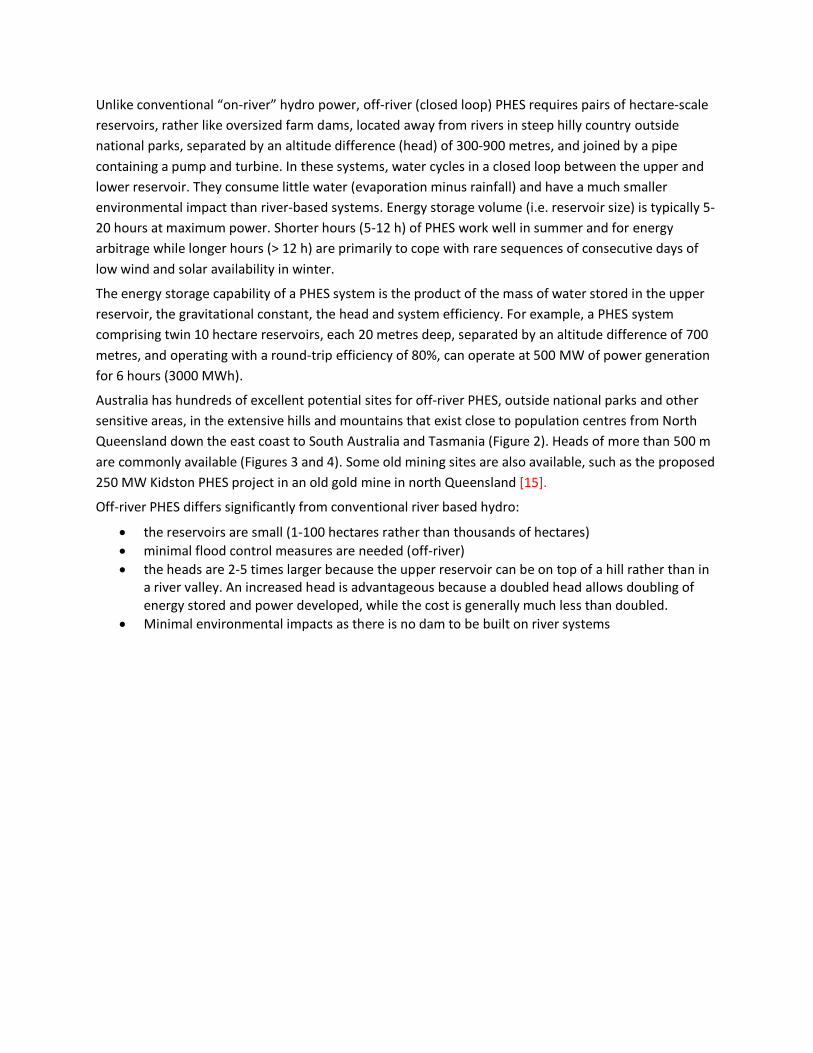
Australia has hundreds of excellent potential sites for off-river PHES, outside national parks and other sensitive areas, in the extensive hills and mountains that exist close to population centres from North Queensland down the east coast to South Australia and Tasmania (Figure 2). Heads of more than 500 m are commonly available (Figures 3 and 4). Some old mining sites are also available, such as the proposed 250 MW Kidston PHES project in an old gold mine in north Queensland [15].

Off-river PHES differs significantly from conventional river based hydro:

• the reservoirs are small (1-100 hectares rather than thousands of hectares) • minimal flood control measures are needed (off-river) • the heads are 2-5 times larger because the upper reservoir can be on top of a hill rather than in

a river valley. An increased head is advantageous because a doubled head allows doubling of energy stored and power developed, while the cost is generally much less than doubled.

• Minimal environmental impacts as there is no dam to be built on river systems

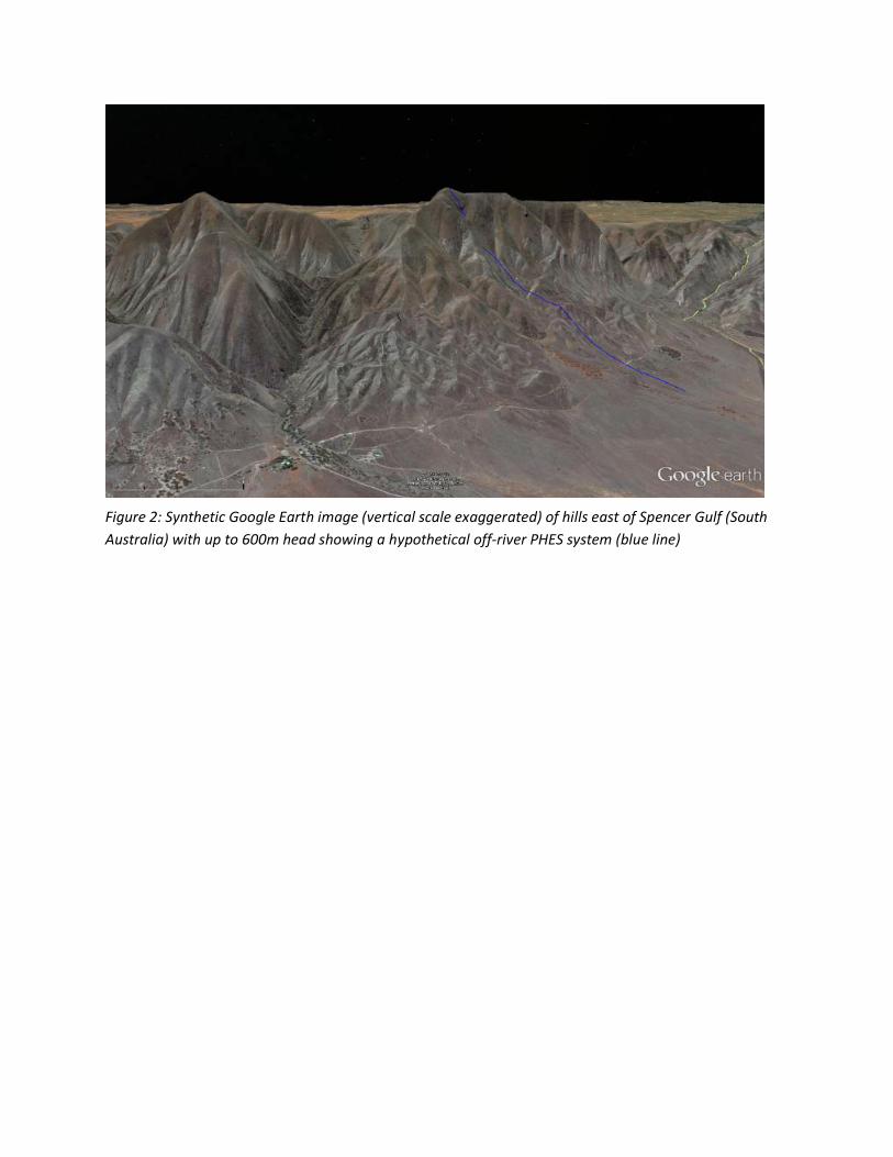
Figure 2: Synthetic Google Earth image (vertical scale exaggerated) of hills east of Spencer Gulf (South Australia) with up to 600m head showing a hypothetical off-river PHES system (blue line)

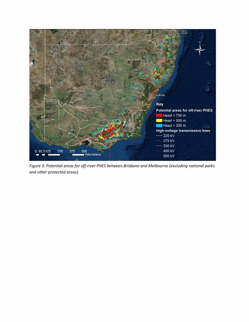
Figure 3: Potential areas for off-river PHES between Brisbane and Melbourne (excluding national parks and other protected areas).

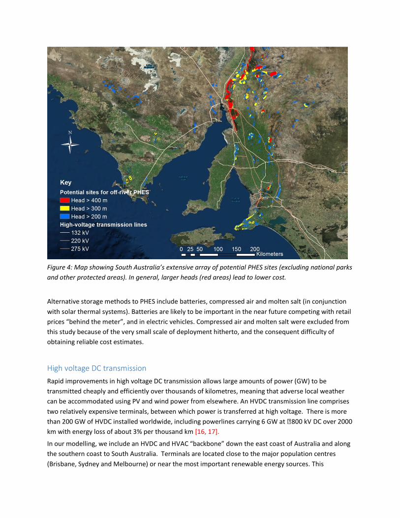
Figure 4: Map showing South Australia’s extensive array of potential PHES sites (excluding national parks and other protected areas). In general, larger heads (red areas) lead to lower cost.

Alternative storage methods to PHES include batteries, compressed air and molten salt (in conjunction with solar thermal systems). Batteries are likely to be important in the near future competing with retail prices “behind the meter”, and in electric vehicles. Compressed air and molten salt were excluded from this study because of the very small scale of deployment hitherto, and the consequent difficulty of obtaining reliable cost estimates.

High voltage DC transmission Rapid improvements in high voltage DC transmission allows large amounts of power (GW) to be transmitted cheaply and efficiently over thousands of kilometres, meaning that adverse local weather can be accommodated using PV and wind power from elsewhere. An HVDC transmission line comprises two relatively expensive terminals, between which power is transferred at high voltage. There is more than 200 GW of HVDC installed worldwide, including powerlines carrying 6 GW at 800 kV DC over 2000 km with energy loss of about 3% per thousand km [16, 17].

In our modelling, we include an HVDC and HVAC “backbone” down the east coast of Australia and along the southern coast to South Australia. Terminals are located close to the major population centres (Brisbane, Sydney and Melbourne) or near the most important renewable energy sources. This

HVDC/HVAC backbone passes within 200 km of three quarters of the Australian population (most of whom live within 50 km of the coast). The existing transmission and distribution system is connected to this HVDC/HVAC system to distribute power to consumers, and to transmit power from PV and wind generators to the HVDC/HVAC interconnector.

Local generation and demand management Australia presently has 1.5 million domestic roof-mounted PV systems (5-6 GW) from a housing stock of about 9 million dwellings (7.3 million in the NEM) [12]. Our modelling recognizes the likelihood of continued substantial growth in privately funded rooftop PV systems. We assume that, in the future, one quarter of dwellings in the NEM are mounted with a fixed 5 kW PV system. Additionally, a similar capacity of solar panels is assumed on commercial building roofs. The total capacity of roof mounted systems is therefore assumed to be 17.3 GW, and based on simulation this yields 23 TWh of annual generation. This is about 11% of annual electricity consumption in the NEM (205 TWh per year).

These PV systems are distributed in the capital cities of each state, where the majority of the population lives. The output of these PV systems is assumed to be preferentially consumed before contributions from any other generator. Hourly demand is reduced by the modelled rooftop generation. The cost of these systems is absorbed by the building owners, and does not directly affect calculated electricity costs under this model. The modelling does include the cost of providing sufficient ground mounted PV, wind, PHES and HVDC/HVAC to provide hourly energy balance for the remaining demand for the entire electricity grid.

Demand management is an important tool for reducing the cost of a power system. Typically, the cost of meeting the “last few percent” of electricity demand (for example, the air conditioning load on a hot summer afternoon) is a large fraction of the total cost of electricity supply. Power demand management tools include interruptible industrial loads, adjusting air conditioning temperature settings, moving domestic and commercial water heating to times of abundant wind and sun, and in the future, managing the timing of household and electric car battery charging and discharging.

In most of our scenarios we meet the NEM reliability standard of no more than 0.002% of unmet load (4 GWh per year) without demand management. However, in other scenarios we assume that demand management is employed during critical periods, which are typically cold wet windless weeks in winter that occur once every few years. During these periods the PHES reservoirs run down to zero over a few days because there is insufficient wind and PV generation to recharge them, leading to a shortfall in supply. The amount of PV, wind and PHES storage could be increased to cover this shortfall. However, this substantial extra investment would be utilised only for a few days every few years.

In some scenarios, we model demand management during critical periods by relaxing the NEM reliability standard. For example, the allowable unmet load might be increased to 336 GWh per 5 year period through contractually agreed load shedding arrangements. In most years demand would be fully met, but every few years this additional shortfall allowance would be utilised. Modern techniques allow cloudy and windless periods to be forecast (thus providing ample warning), and the PHES storages represent a substantial buffer. A portion of the savings in investment in PV, wind and PHES would be available to compensate certain consumers for partial loss of supply for a few days every few years. For

example, reducing the overall cost of electricity supply by $2/MWh by allowing an unmet load of 336 GWh per 5 years would save $2 billion per 5 years, which is equivalent to $6,000 per unmet MWh.

Stability of the NEM In our study, we model scenarios in which the National Electricity Market is exclusively supplied by renewable energy, with most of this generation having limited controllability. PV and wind can be rapidly curtailed, but cannot be increased at will unless operating in a curtailed mode. Variable wind and solar power supply must be balanced with the uncontrolled (but reasonably predictable) instantaneous demand for electricity in real time.

The dynamical behaviour (on time scales of sub-seconds to minutes) of a 100% renewable energy grid is outside the scope of the present study. PV and wind are variable generators and lack the inertial energy storage possessed by conventional fossil, nuclear and hydro generators. However, this does not mean that a renewable electricity grid will be inherently less reliable than an equivalent fossil fuelled system. As previously noted, PHES can provide excellent inertial energy storage, very fast response time (typically 1% per second) and black start capability (to restore a collapsed grid).

Hundreds of wind and PV farms are statistically more reliable than several large fossil fuel power stations because breakdowns of individual generators have only a small effect on overall output. Wide distribution of wind, PV and PHES means that collapse of major transmission lines need not bring down local supply.

Solar and wind forecasting skill is already very good, and continues to improve. The combined output of thousands of wind and PV systems distributed over tens of millions of hectares can be predicted on every time scale from seconds to years. Even a fast-moving weather event takes hours or days to move over a significant fraction of the PV and wind generators (and thus affect generation). This allows ample time for supporting measures to be taken in the event of widespread adverse weather conditions [18], such as moderating demand or drawing energy from storage. Furthermore, the output of wind and PV systems is often counter-correlated - for example, cloudy weather is often windy.

Environmental considerations The area of land required for large scale off-river PHES is small. For example, 20 GW of PHES capacity with 20 hours of storage (400 GWh), a head of 600 m and depth of 20 m requires a total reservoir area (upper and lower) of 36 km2. This represents 5 parts per million of the Australian land mass, and is far smaller than the existing area of artificial reservoirs.

We have identified many potential sites and it will not be necessary to intrude upon national parks and other protected land.

Average annual evaporation in southern states is 1200-1800 mm and the annual rainfall ranges from 500-1000 mm in the Great Diving Range area [19, 20]. Initial fill water will be transported from nearby water sources by pipelines or channels. Micro-catchments around the reservoirs can be built to collect rainwater maintaining the balance between rainfall and evaporation plus leakage. In addition, various

evaporation and leakage reduction measures such as floating covers can be used to mitigate water loss by up to 95% [21].

Taking total reservoir area of 36 km2, and an excess of evaporation over rainfall of 300 mm per year, the annual water requirement is 11 GL. This represents 0.3% of current water extraction from rivers under Murray Darling Basin Authority (MDBA) control. The cost of this water at commercial prices is small relative to other costs.

Economic parameters We calculate the levelised cost of energy (LCOE) using a real (i.e. inflation-free) discount rate of 5% per year. This includes bank finance for 70% of capital expenditure at a nominal rate of 5% per year, a return on investment of 10% (nominal) on equity (30% of capital expenditure) and an inflation rate of 1.5% per year. The Reserve Bank of Australia cash rate is currently 1.5% per year. We use Australian dollars and an exchange rate of AU$1.00 = US$0.75.

Our cost estimates pertain to 2016 costs in Australia. Our cost estimates of PV, wind and PHES in Table 1 are derived from the following sources: PV: Data for the current cost of PV in Australia comes from the Australian Renewable Energy Agency (ARENA) large scale solar grant round. Approximately 600 MWDC will be supported by ARENA, to be constructed during 2017. Most of the PV comprises single axis tracking systems located in Queensland and New South Wales, in the 15-50 MW range, at a cost of $1800 per kW. In view of the recent rapid fall in PV module prices, a figure of $1700/kW is used in our modelling. The DC capacity factor is around 23%, the lifetime is 25 years and the cost of operations and maintenance is $20/MWh [22]. This yields an LCOE of $78/MWh.

Wind: The Government of the Australian Capital Territory (ACT) recently conducted three public reverse auctions which resulted in the contracting of the output of 600 MW of new windfarms. The energy price for each contract is a fixed number (no allowance for inflation). The price (after adjusting for inflation) is equivalent to $64/MWh. The figures presented in Table 1 are consistent with this figure using an assumed average capacity factor of 41%.

Our cost estimates do not include a carbon price or subsidies. PV and wind costs are very likely to continue to fall.

PHES: A private cost model is used, developed by an experienced hydro engineer based upon existing models. The model has been tested for consistency with publicly available PHES systems costs. The unit off-river PHES system is assumed to have a power of 200 MW, a head of 600 m, twin 20 m deep 5 hectare “turkey nest” ponds with earth walls built on flat land, penstock slope of 13 degrees, easy access, minimal flood control measures and a round trip efficiency of 80%. The estimated cost is $800 per kW (for penstocks, machinery and power conversion) and $70 per kWh (for pond excavation and construction), with scaling factors applied for different head and pond size. Head is a strong inverse driver of cost of storage. Transmission to a high voltage node is an additional cost and calculated separately.

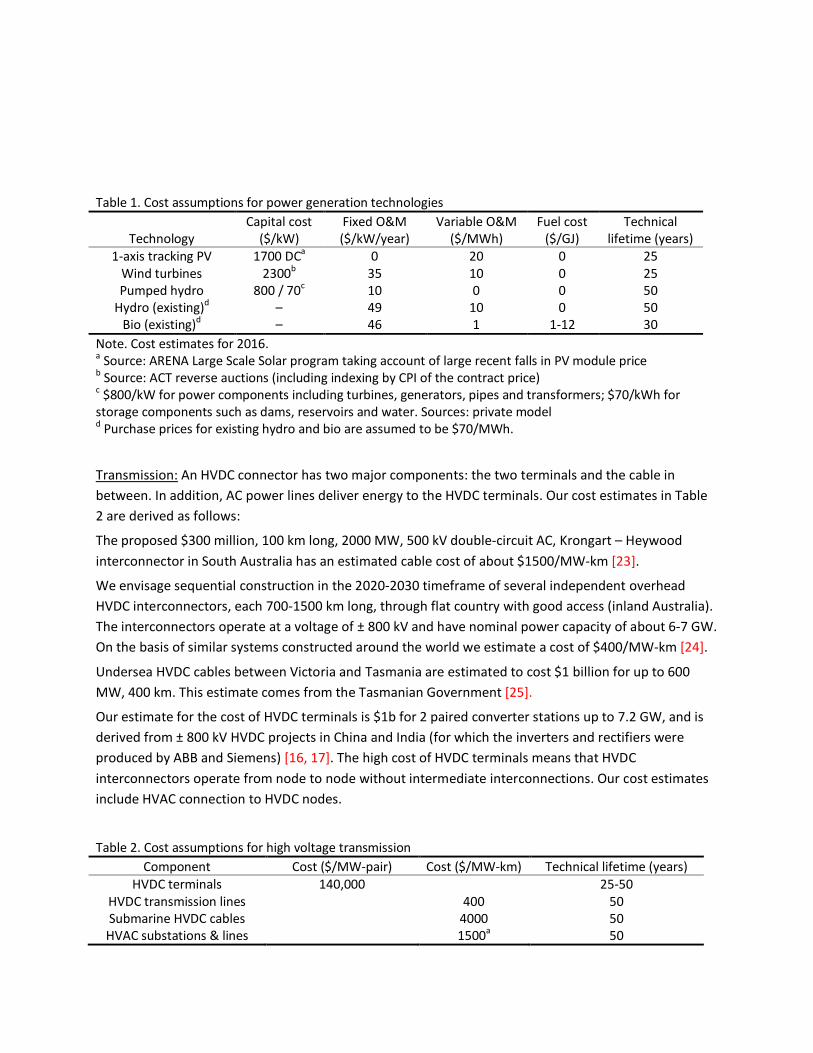
Table 1. Cost assumptions for power generation technologies

Technology Capital cost

($/kW) Fixed O&M ($/kW/year)

Variable O&M ($/MWh)

Fuel cost ($/GJ)

Technical lifetime (years)

1-axis tracking PV 1700 DCa 0 20 0 25 Wind turbines 2300b 35 10 0 25 Pumped hydro 800 / 70c 10 0 0 50

Hydro (existing)d – 49 10 0 50 Bio (existing)d – 46 1 1-12 30

Note. Cost estimates for 2016. a Source: ARENA Large Scale Solar program taking account of large recent falls in PV module price b Source: ACT reverse auctions (including indexing by CPI of the contract price) c $800/kW for power components including turbines, generators, pipes and transformers; $70/kWh for storage components such as dams, reservoirs and water. Sources: private model d Purchase prices for existing hydro and bio are assumed to be $70/MWh.

Transmission: An HVDC connector has two major components: the two terminals and the cable in between. In addition, AC power lines deliver energy to the HVDC terminals. Our cost estimates in Table 2 are derived as follows:

The proposed $300 million, 100 km long, 2000 MW, 500 kV double-circuit AC, Krongart – Heywood interconnector in South Australia has an estimated cable cost of about $1500/MW-km [23].

We envisage sequential construction in the 2020-2030 timeframe of several independent overhead HVDC interconnectors, each 700-1500 km long, through flat country with good access (inland Australia). The interconnectors operate at a voltage of ± 800 kV and have nominal power capacity of about 6-7 GW. On the basis of similar systems constructed around the world we estimate a cost of $400/MW-km [24].

Undersea HVDC cables between Victoria and Tasmania are estimated to cost $1 billion for up to 600 MW, 400 km. This estimate comes from the Tasmanian Government [25].

Our estimate for the cost of HVDC terminals is $1b for 2 paired converter stations up to 7.2 GW, and is derived from ± 800 kV HVDC projects in China and India (for which the inverters and rectifiers were produced by ABB and Siemens) [16, 17]. The high cost of HVDC terminals means that HVDC interconnectors operate from node to node without intermediate interconnections. Our cost estimates include HVAC connection to HVDC nodes.

Table 2. Cost assumptions for high voltage transmission Component Cost ($/MW-pair) Cost ($/MW-km) Technical lifetime (years)

HVDC terminals 140,000 25-50 HVDC transmission lines 400 50 Submarine HVDC cables 4000 50

HVAC substations & lines 1500a 50

Note. Cost estimates for 2016. a assuming 50 km for wind farms and PHES, 10 km for solar farms located in existing transmission zones and 150 km for the inland regions. Cable lifetime: 50 years; terminal lifetime: 25 years

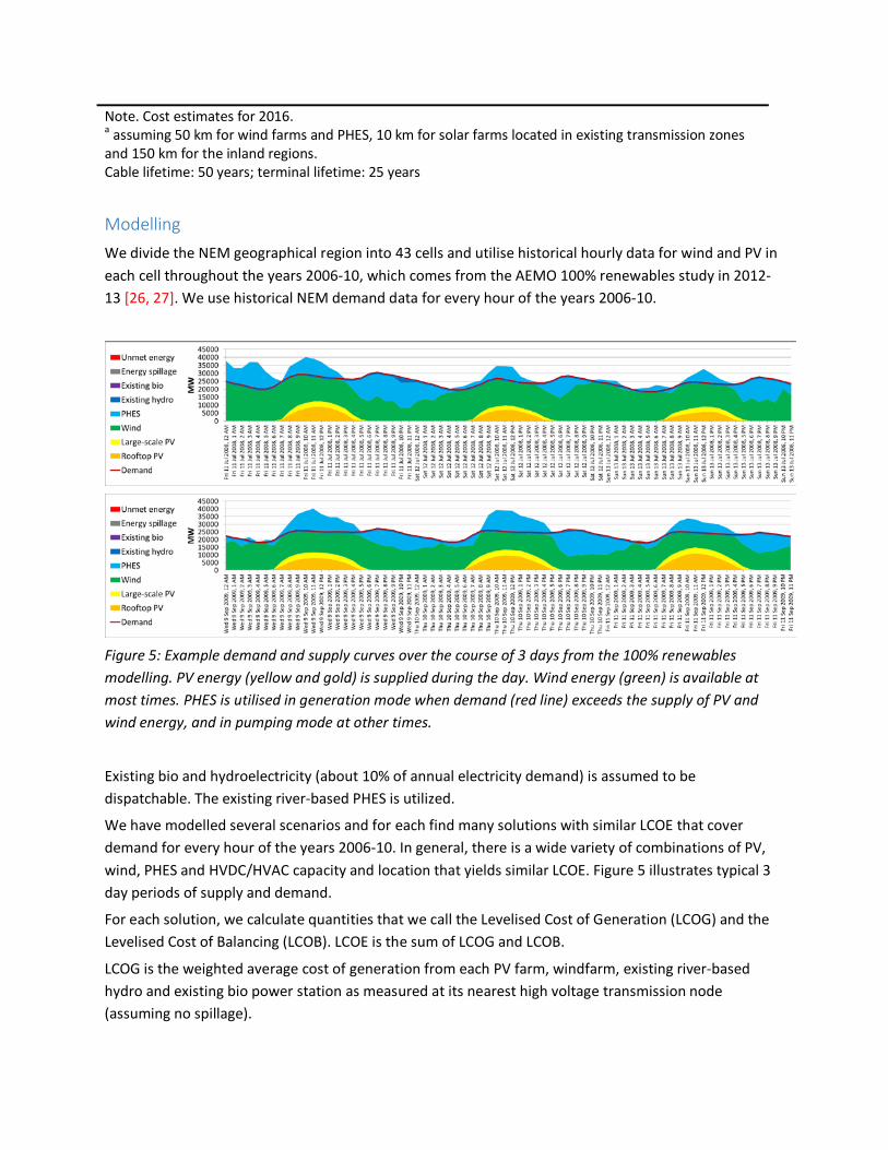
Modelling We divide the NEM geographical region into 43 cells and utilise historical hourly data for wind and PV in each cell throughout the years 2006-10, which comes from the AEMO 100% renewables study in 2012-13 [26, 27]. We use historical NEM demand data for every hour of the years 2006-10.

Figure 5: Example demand and supply curves over the course of 3 days from the 100% renewables modelling. PV energy (yellow and gold) is supplied during the day. Wind energy (green) is available at most times. PHES is utilised in generation mode when demand (red line) exceeds the supply of PV and wind energy, and in pumping mode at other times.

Existing bio and hydroelectricity (about 10% of annual electricity demand) is assumed to be dispatchable. The existing river-based PHES is utilized.

We have modelled several scenarios and for each find many solutions with similar LCOE that cover demand for every hour of the years 2006-10. In general, there is a wide variety of combinations of PV, wind, PHES and HVDC/HVAC capacity and location that yields similar LCOE. Figure 5 illustrates typical 3 day periods of supply and demand.

For each solution, we calculate quantities that we call the Levelised Cost of Generation (LCOG) and the Levelised Cost of Balancing (LCOB). LCOE is the sum of LCOG and LCOB.

LCOG is the weighted average cost of generation from each PV farm, windfarm, existing river-based hydro and existing bio power station as measured at its nearest high voltage transmission node (assuming no spillage).

LCOB comprises the capital and operations costs of PHES and HVDC/HVAC, round trip energy losses in PHES systems, resistive losses in HVDC/HVAC systems, and spillage of excess PV and wind energy during sunny and windy periods when storages are full (i.e. the cost of building excess wind and PV). For small penetrations of PV and wind LCOB is approximately zero and LCOE and LCOG are approximately equal. For large penetrations LCOB becomes significant to cover the cost of coping with the variability of PV and wind.

In general, LCOB is minimized by utilizing PHES to store excess energy for later use (and thus minimize spillage), and by distributing PV and wind very widely using HVDC/HVAC (to take advantage of different weather systems in different regions). In some regions the output of PV and wind are counter-correlated and so utilization of both can reduce LCOB.

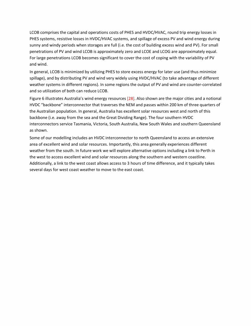
Figure 6 illustrates Australia’s wind energy resources [28]. Also shown are the major cities and a notional HVDC “backbone” interconnector that traverses the NEM and passes within 200 km of three quarters of the Australian population. In general, Australia has excellent solar resources west and north of this backbone (i.e. away from the sea and the Great Dividing Range). The four southern HVDC interconnectors service Tasmania, Victoria, South Australia, New South Wales and southern Queensland as shown.

Some of our modelling includes an HVDC interconnector to north Queensland to access an extensive area of excellent wind and solar resources. Importantly, this area generally experiences different weather from the south. In future work we will explore alternative options including a link to Perth in the west to access excellent wind and solar resources along the southern and western coastline. Additionally, a link to the west coast allows access to 3 hours of time difference, and it typically takes several days for west coast weather to move to the east coast.

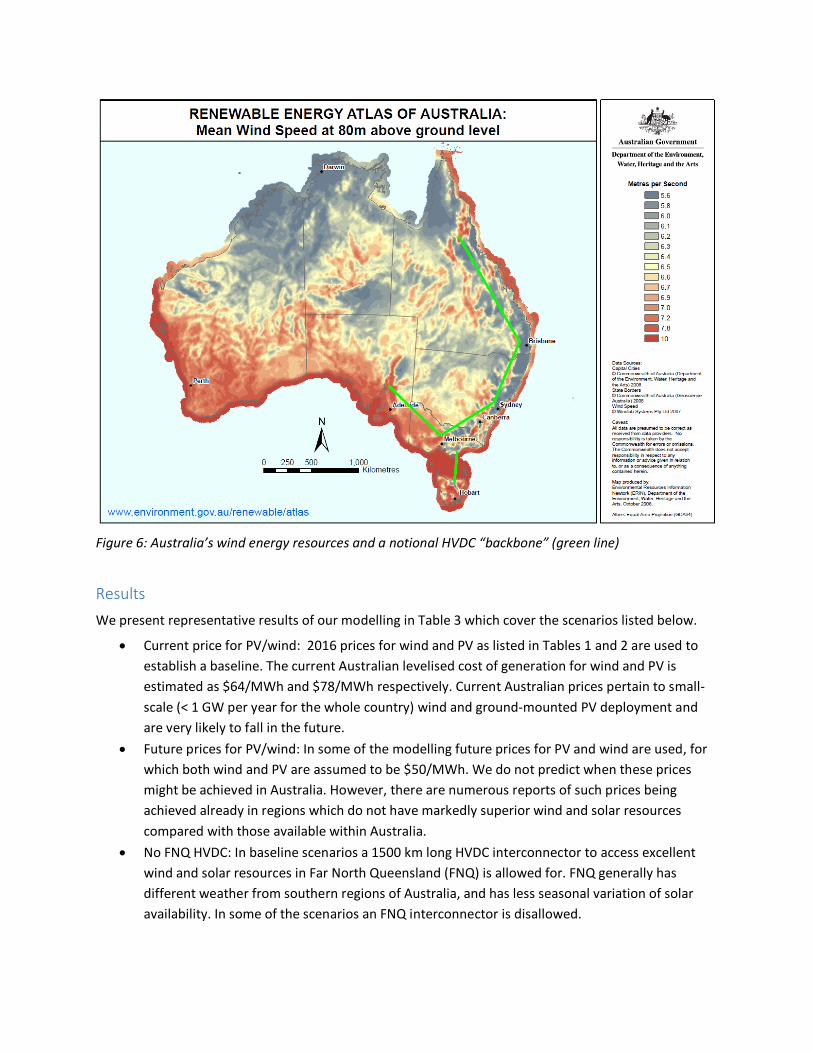
Figure 6: Australia’s wind energy resources and a notional HVDC “backbone” (green line)

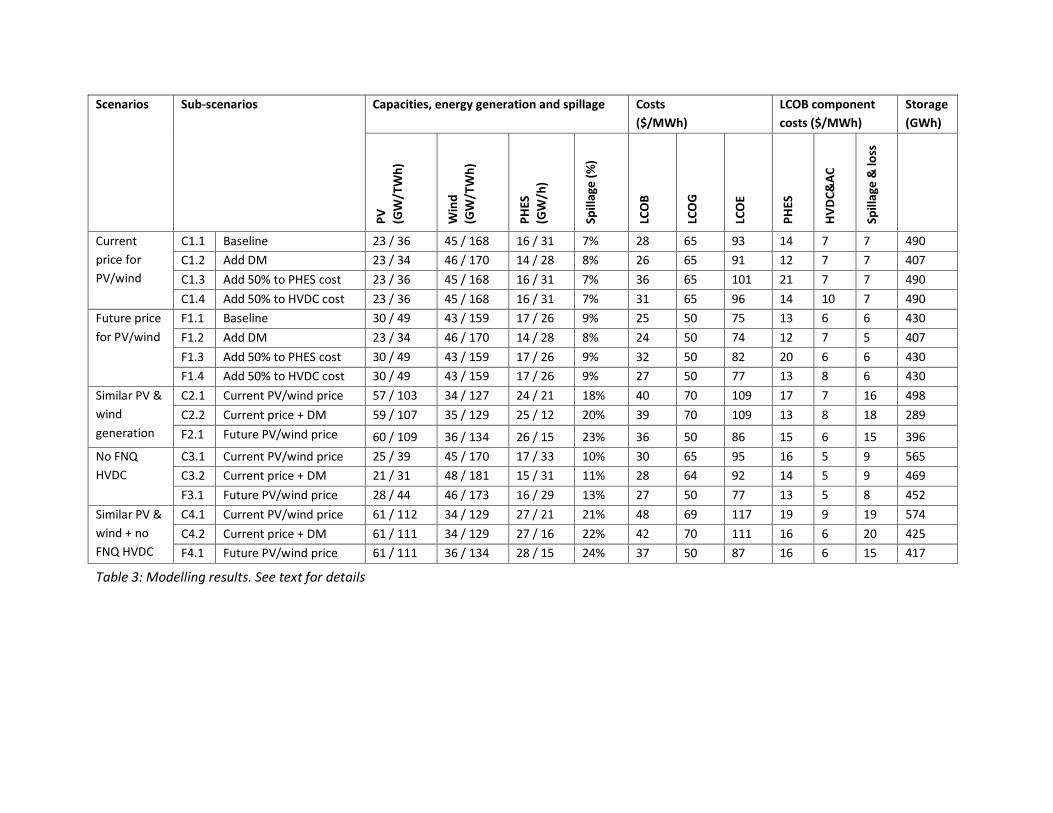
Results We present representative results of our modelling in Table 3 which cover the scenarios listed below.

• Current price for PV/wind: 2016 prices for wind and PV as listed in Tables 1 and 2 are used to establish a baseline. The current Australian levelised cost of generation for wind and PV is estimated as $64/MWh and $78/MWh respectively. Current Australian prices pertain to small-scale (< 1 GW per year for the whole country) wind and ground-mounted PV deployment and are very likely to fall in the future.

• Future prices for PV/wind: In some of the modelling future prices for PV and wind are used, for which both wind and PV are assumed to be $50/MWh. We do not predict when these prices might be achieved in Australia. However, there are numerous reports of such prices being achieved already in regions which do not have markedly superior wind and solar resources compared with those available within Australia.

• No FNQ HVDC: In baseline scenarios a 1500 km long HVDC interconnector to access excellent wind and solar resources in Far North Queensland (FNQ) is allowed for. FNQ generally has different weather from southern regions of Australia, and has less seasonal variation of solar availability. In some of the scenarios an FNQ interconnector is disallowed.

• Similar PV and wind generation: In the baseline scenarios, the relative proportions of annual wind and PV generation is unconstrained. In some of the scenarios the annual amount of wind and PV generation is constrained to be similar

We also present several sub-scenarios in addition to the baseline case.

• Demand management (DM): In baseline scenarios the unmet demand standard for the NEM (4 GWh per year, 0.002% of annual energy) is adhered to. In some scenarios this standard is relaxed through voluntary curtailment of demand by 2 GW (about 5% of peak demand) for 7 days over 5 years. This corresponds to an unmet demand of 336 GWh over 5 years (0.033% of annual energy).

• Add 50% to PHES or HVDC costs: Some sub-scenarios are modelling with 50% higher HVDC or PHES costs to test the sensitivity of the model to these cost inputs.

In each scenario rooftop PV power and energy generation amounts to 17 GW and 23 TWh/year respectively. Generation from existing bio and hydro amounts to 17-20 TWh per year and is purchased at a price of $70/MWh for current (2016) scenarios and $50/MWh for future scenarios. Annual electricity consumption is assumed to be constant at 205 TWh per year (corresponding to an average demand of 23 GW). Peak demand is assumed to remain at 35 GW.

For each scenario Table 3 shows optimised amounts of PV and wind in terms of power capacity (GW) and annual generation (TWh). The optimised PHES power capacity (GW) and hours of storage (h) at that capacity is also shown. The levelised cost of Balancing (LCOB), Generation (LCOG) and Energy (LCOE) is shown, together with the LCOB components. The total optimised storage (GWh) is shown, which is the product of capacity and hours of storage.

Scenarios Sub-scenarios Capacities, energy generation and spillage Costs ($/MWh)

LCOB component costs ($/MWh)

Storage (GWh)

PV

(GW

/TW

h)

Win

d (G

W/T

Wh)

PHES

(G

W/h

)

Spill

age

(%)

LCO

B

LCO

G

LCO

E

PHES

HVD

C&AC

Spill

age

& lo

ss

Current price for PV/wind

C1.1 Baseline 23 / 36 45 / 168 16 / 31 7% 28 65 93 14 7 7 490 C1.2 Add DM 23 / 34 46 / 170 14 / 28 8% 26 65 91 12 7 7 407 C1.3 Add 50% to PHES cost 23 / 36 45 / 168 16 / 31 7% 36 65 101 21 7 7 490 C1.4 Add 50% to HVDC cost 23 / 36 45 / 168 16 / 31 7% 31 65 96 14 10 7 490

Future price for PV/wind

F1.1 Baseline 30 / 49 43 / 159 17 / 26 9% 25 50 75 13 6 6 430 F1.2 Add DM 23 / 34 46 / 170 14 / 28 8% 24 50 74 12 7 5 407 F1.3 Add 50% to PHES cost 30 / 49 43 / 159 17 / 26 9% 32 50 82 20 6 6 430 F1.4 Add 50% to HVDC cost 30 / 49 43 / 159 17 / 26 9% 27 50 77 13 8 6 430

Similar PV & wind generation

C2.1 Current PV/wind price 57 / 103 34 / 127 24 / 21 18% 40 70 109 17 7 16 498 C2.2 Current price + DM 59 / 107 35 / 129 25 / 12 20% 39 70 109 13 8 18 289 F2.1 Future PV/wind price 60 / 109 36 / 134 26 / 15 23% 36 50 86 15 6 15 396

No FNQ HVDC

C3.1 Current PV/wind price 25 / 39 45 / 170 17 / 33 10% 30 65 95 16 5 9 565 C3.2 Current price + DM 21 / 31 48 / 181 15 / 31 11% 28 64 92 14 5 9 469 F3.1 Future PV/wind price 28 / 44 46 / 173 16 / 29 13% 27 50 77 13 5 8 452

Similar PV & wind + no FNQ HVDC

C4.1 Current PV/wind price 61 / 112 34 / 129 27 / 21 21% 48 69 117 19 9 19 574 C4.2 Current price + DM 61 / 111 34 / 129 27 / 16 22% 42 70 111 16 6 20 425 F4.1 Future PV/wind price 61 / 111 36 / 134 28 / 15 24% 37 50 87 16 6 15 417

Table 3: Modelling results. See text for details

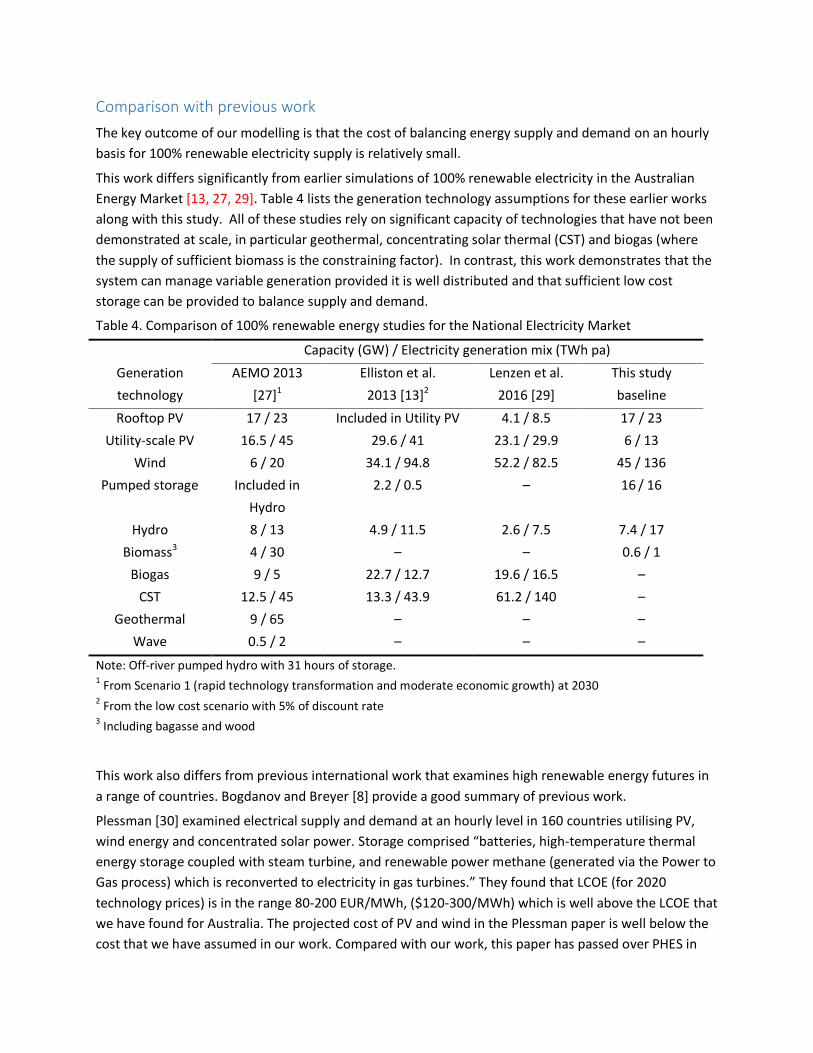
Comparison with previous work The key outcome of our modelling is that the cost of balancing energy supply and demand on an hourly basis for 100% renewable electricity supply is relatively small.

This work differs significantly from earlier simulations of 100% renewable electricity in the Australian Energy Market [13, 27, 29]. Table 4 lists the generation technology assumptions for these earlier works along with this study. All of these studies rely on significant capacity of technologies that have not been demonstrated at scale, in particular geothermal, concentrating solar thermal (CST) and biogas (where the supply of sufficient biomass is the constraining factor). In contrast, this work demonstrates that the system can manage variable generation provided it is well distributed and that sufficient low cost storage can be provided to balance supply and demand.

Table 4. Comparison of 100% renewable energy studies for the National Electricity Market

Capacity (GW) / Electricity generation mix (TWh pa) Generation technology

AEMO 2013 [27]1

Elliston et al. 2013 [13]2

Lenzen et al. 2016 [29]

This study baseline

Rooftop PV 17 / 23 Included in Utility PV 4.1 / 8.5 17 / 23 Utility-scale PV 16.5 / 45 29.6 / 41 23.1 / 29.9 6 / 13

Wind 6 / 20 34.1 / 94.8 52.2 / 82.5 45 / 136 Pumped storage Included in

Hydro 2.2 / 0.5 – 16 / 16

Hydro 8 / 13 4.9 / 11.5 2.6 / 7.5 7.4 / 17 Biomass3 4 / 30 – – 0.6 / 1

Biogas 9 / 5 22.7 / 12.7 19.6 / 16.5 – CST 12.5 / 45 13.3 / 43.9 61.2 / 140 –

Geothermal 9 / 65 – – – Wave 0.5 / 2 – – –

Note: Off-river pumped hydro with 31 hours of storage. 1 From Scenario 1 (rapid technology transformation and moderate economic growth) at 2030 2 From the low cost scenario with 5% of discount rate 3 Including bagasse and wood

This work also differs from previous international work that examines high renewable energy futures in a range of countries. Bogdanov and Breyer [8] provide a good summary of previous work.

Plessman [30] examined electrical supply and demand at an hourly level in 160 countries utilising PV, wind energy and concentrated solar power. Storage comprised “batteries, high-temperature thermal energy storage coupled with steam turbine, and renewable power methane (generated via the Power to Gas process) which is reconverted to electricity in gas turbines.” They found that LCOE (for 2020 technology prices) is in the range 80-200 EUR/MWh, ($120-300/MWh) which is well above the LCOE that we have found for Australia. The projected cost of PV and wind in the Plessman paper is well below the cost that we have assumed in our work. Compared with our work, this paper has passed over PHES in

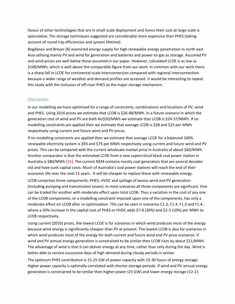
favour of other technologies that are in small scale deployment and hence their cost at large scale is speculative. The storage techniques suggested are considerably more expensive than PHES (taking account of round trip efficiencies and system lifetime).

Bogdanov and Breyer [8] examined energy supply for high renewable energy penetration in north east Asia utilising mainly PV and wind for generation and batteries and power-to-gas as storage. Assumed PV and wind prices are well below those assumed in our paper. However, calculated LCOE is as low as $100/MWh, which is well above the comparable figure from our work. In common with our work there is a sharp fall in LCOE for continental-scale interconnection compared with regional interconnection because a wider range of weather and demand profiles are accessed. It would be interesting to repeat this study with the inclusion of off-river PHES as the major storage mechanism.

Discussion In our modelling we have optimised for a range of constraints, combinations and locations of PV, wind and PHES. Using 2016 prices we estimate that LCOB is $26-48/MWh. In a future scenario in which the generation cost of wind and PV are both AU$50/MWh we estimate that LCOB is $24-37/MWh. If no modelling constraints are applied then we estimate that average LCOB is $28 and $25 per MWh respectively using current and future wind and PV prices.

If no modelling constraints are applied then we estimate that average LCOE for a balanced 100% renewable electricity system is $93 and $75 per MWh respectively using current and future wind and PV prices. This can be compared with the current wholesale market price in Australia of about $60/MWh. Another comparator is that the estimated LCOE from a new supercritical black coal power station in Australia is $80/MWh [31]. The current NEM contains mostly coal generators that are several decades old and have sunk capital costs. Much of Australia’s coal power stations will reach the end of their economic life over the next 15 years. It will be cheaper to replace these with renewable energy.

LCOB comprises three components: PHES, HVDC and spillage of excess wind and PV generation (including pumping and transmission losses). In most scenarios all three components are significant. One can be traded for another with moderate effect upon total LCOB. Thus a variation in the cost of any one of the LCOB components, or a modelling constraint imposed upon one of the components, has only a moderate effect on LCOB after re-optimisation. This can be seen in scenarios C1.3, C1.4, F1.3 and F1.4, where a 50% increase in the capital cost of PHES or HVDC adds $7-8 (30%) and $2-3 (10%) per MWh to LCOB respectively.

Using current (2016) prices, the lowest LCOE is for scenarios in which wind produces most of the energy because wind energy is significantly cheaper than PV at present. The lowest LCOB is also for scenarios in which wind produces most of the energy for both current and future wind and PV price scenarios. If wind and PV annual energy generation is constrained to be similar then LCOB rises by about $11/MWh. The advantage of wind is that it can deliver energy at any time, rather than only during the day. Wind is better able to service successive days of high demand during cloudy periods in winter.

The optimum PHES contribution is 15-25 GW of power capacity with 15-30 hours of energy storage. Higher power capacity is optimally correlated with shorter storage periods. If wind and PV annual energy generation is constrained to be similar then higher power (25 GW) and lower energy storage (12-21

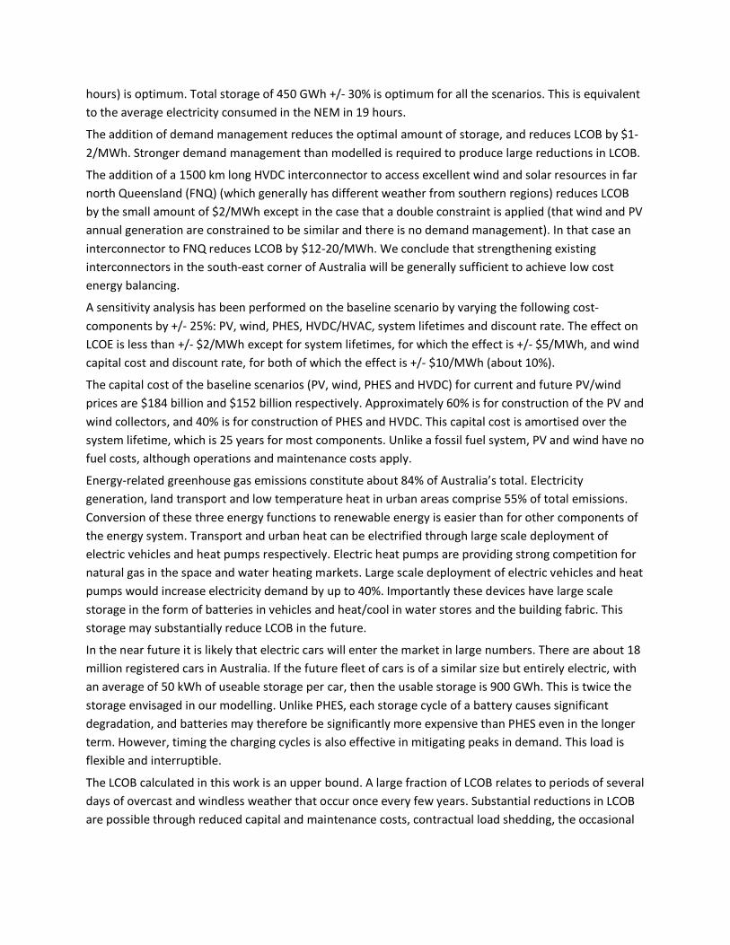
hours) is optimum. Total storage of 450 GWh +/- 30% is optimum for all the scenarios. This is equivalent to the average electricity consumed in the NEM in 19 hours.

The addition of demand management reduces the optimal amount of storage, and reduces LCOB by $1-2/MWh. Stronger demand management than modelled is required to produce large reductions in LCOB.

The addition of a 1500 km long HVDC interconnector to access excellent wind and solar resources in far north Queensland (FNQ) (which generally has different weather from southern regions) reduces LCOB by the small amount of $2/MWh except in the case that a double constraint is applied (that wind and PV annual generation are constrained to be similar and there is no demand management). In that case an interconnector to FNQ reduces LCOB by $12-20/MWh. We conclude that strengthening existing interconnectors in the south-east corner of Australia will be generally sufficient to achieve low cost energy balancing.

A sensitivity analysis has been performed on the baseline scenario by varying the following cost-components by +/- 25%: PV, wind, PHES, HVDC/HVAC, system lifetimes and discount rate. The effect on LCOE is less than +/- $2/MWh except for system lifetimes, for which the effect is +/- $5/MWh, and wind capital cost and discount rate, for both of which the effect is +/- $10/MWh (about 10%).

The capital cost of the baseline scenarios (PV, wind, PHES and HVDC) for current and future PV/wind prices are $184 billion and $152 billion respectively. Approximately 60% is for construction of the PV and wind collectors, and 40% is for construction of PHES and HVDC. This capital cost is amortised over the system lifetime, which is 25 years for most components. Unlike a fossil fuel system, PV and wind have no fuel costs, although operations and maintenance costs apply.

Energy-related greenhouse gas emissions constitute about 84% of Australia’s total. Electricity generation, land transport and low temperature heat in urban areas comprise 55% of total emissions. Conversion of these three energy functions to renewable energy is easier than for other components of the energy system. Transport and urban heat can be electrified through large scale deployment of electric vehicles and heat pumps respectively. Electric heat pumps are providing strong competition for natural gas in the space and water heating markets. Large scale deployment of electric vehicles and heat pumps would increase electricity demand by up to 40%. Importantly these devices have large scale storage in the form of batteries in vehicles and heat/cool in water stores and the building fabric. This storage may substantially reduce LCOB in the future.

In the near future it is likely that electric cars will enter the market in large numbers. There are about 18 million registered cars in Australia. If the future fleet of cars is of a similar size but entirely electric, with an average of 50 kWh of useable storage per car, then the usable storage is 900 GWh. This is twice the storage envisaged in our modelling. Unlike PHES, each storage cycle of a battery causes significant degradation, and batteries may therefore be significantly more expensive than PHES even in the longer term. However, timing the charging cycles is also effective in mitigating peaks in demand. This load is flexible and interruptible.

The LCOB calculated in this work is an upper bound. A large fraction of LCOB relates to periods of several days of overcast and windless weather that occur once every few years. Substantial reductions in LCOB are possible through reduced capital and maintenance costs, contractual load shedding, the occasional

use of legacy coal and gas generators to charge the PHES reservoirs, household battery storage and management of the charging times of batteries in electric cars.

It will take some time for wind and PV penetration to reach into the range 50-100% of annual energy in the NEM, and so the future price scenarios are more relevant than current price scenarios. With PV and wind in the price range of $50/MWh, the LCOE of a balanced 100% renewable electricity system is around $75/MWh. This is below the LCOE of any alternative supply option, and is close to the current NEM pool price. A future carbon price will tip the balance further in favour of an all-renewable energy system. Further modelling is likely to refine costs and uncover improved solutions that lead to lower LCOB.

In our work we used demand, wind and solar data for the 5-year period 2006-10. In future work we will extend this period to 15 years using historical records, and for considerably longer using synthetic data sets where necessary.

In our modelling we avoid heroic assumptions about future technology development by only including technology that has already been deployed in large quantities around the world (> 100 GW), namely PV, wind, HVDC/HVAC and PHES. This means that our cost estimates are more robust than for models that utilise technology projections that are far beyond current practice.

The relatively low LCOE that we calculate for balanced supply of 100% renewable electricity based upon wind and PV, coupled with the large scale of these manufacturing industries, suggests that wind and PV will dominate the Australian grid in the future. PHES and HVDC/HVAC offers an effective and low cost solution to the variability of wind and PV. Unlike the case of molten salt energy storage or biomass energy balancing, excess wind energy can be stored in a PHES system to reduce spillage with only small loss (80% round trip efficiency).

In the view of the authors, it will be difficult for any other low emission technology (such as nuclear, solar thermal, geothermal, ocean and biomass) to become competitive, neither on the basis of competitive supply of energy alone nor on the basis of supply of both energy and ancillary balancing services.

Acknowledgements Support from the Australian Renewable Energy Agency (ARENA) for PHES site searching and the development of cost models for PHES is gratefully acknowledged. Responsibility for the views, information or advice expressed herein is not accepted by the Australian Government.

References 1. REN21, Renewables 2016 global status report. 2016, Paris: REN21 Secretariat. 2. Frankfurt School-UNEP Centre/BNEF, Global trends in renewable energy investment 2015. 2015. 3. International Renewable Energy Agency, Renewable capacity statistics 2016. 2016. 4. Australian Bureau of Resources and Energy Economics, Australian Energy Resource Assessment.

2014. p. 311-336. 5. Blakers, A., Sustainable Energy Options. Asian Perspective, 2015. 39(4): p. 559-589.

6. ABC News. Hazelwood power station closure the latest blow for coal. 2016; Available from: http://www.abc.net.au/news/2016-11-03/hazelwood-power-station-closure-blow-to-coal/7992346.

7. ACIL Allen Consulting, Electricity sector emissions: Modelling of the Australian electricity generation sector. 2013. p. 9-15.

8. Bogdanov, D. and C. Breyer, North-East Asian Super Grid for 100% renewable energy supply: Optimal mix of energy technologies for electricity, gas and heat supply options. Energy Conversion and Management, 2016. 112: p. 176-190.

9. Australian Energy Market Operator. AEMO undertakes role of energy market operator and power system operator in Western Australia. 2015; Available from: https://www.aemo.com.au/-/media/Files/PDF/20150930-AEMO-media-release_-WA-functions.ashx.

10. Australian Energy Regulator. National Electricity Market electricity consumption. 2016; Available from: https://www.aer.gov.au/wholesale-markets/wholesale-statistics/national-electricity-market-electricity-consumption.

11. Teske, S., Dominish, E., Ison, N. and Maras, K., 100% Renewable Energy for Australia – Decarbonising Australia’s Energy Sector within one Generation. 2016.

12. Australian Clean Energy Council, Clean Energy Australia Report 2015. 2016. 13. Elliston, B., L. MacGill, and M. Diesendorf, Least cost 100% renewable electricity scenarios in the

Australian National Electricity Market. Energy Policy, 2013. 59: p. 270-282. 14. Elliston, B., J. Riesz, and L. MacGill, What cost for more renewables? The incremental cost of

renewable generation - An Australian National Electricity Market case study. Renewable Energy, 2016. 95: p. 127-139.

15. Genex Power. The Kidston Hydro Project. 2016; Available from: http://www.genexpower.com.au/the-kidston-hydro-project.html.

16. ABB Group. Xiangjiaba - Shanghai: The world's most powerful and longest ultra high voltage direct current project to go into commercial operation. 2010; Available from: http://new.abb.com/systems/hvdc/references/xiangjiaba---shanghai.

17. ABB Group. ABB selected to provide link worth $900 million for power superhighway in India. 2011; Available from: http://www.abb.com/cawp/seitp202/3e7cf36bde0acd51c125785c00397549.aspx.

18. Australian Energy Market Operator, Australian wind energy forecasting system (AWEFS). 2016. 19. Australian Bureau of Meteorology. Average annual, seasonal and monthly rainfall. 2016;

Available from: http://www.bom.gov.au/jsp/ncc/climate_averages/rainfall/index.jsp. 20. Australian Bureau of Meteorology. Evaporation: Average monthly & annual evaporation. 2016;

Available from: http://www.bom.gov.au/watl/evaporation/. 21. Land & Water Australia. Water storage evaporation. 2016; Available from:

http://lwa.gov.au/national-program-sustainable-irrigation/water-storage-evaporation. 22. Australian Renewable Energy Agency, ARENA large-scale solar PV competitive round: EOI

Application Data. 2016. p. 4-5. 23. ElectraNet, South Australia - Victoria (Heywood) interconnector upgrade RIT-T: Project

assessment conclusions report. 2013. 24. Black & Veatch, Capital costs for transmission and substations - Updated recommendations for

WECC transmission expansion planning. 2014.

25. ABC News. Election 2016: Second undersea cable to Tasmania proposed by both major parties. 2016; Available from: http://www.abc.net.au/news/2016-06-22/second-undersea-cable-to-tasmania-proposed-by-both-major-parties/7531246.

26. Australian Energy Market Operator, 100 per cent renewables study - Modelling assumptions and input. 2012.

27. Australian Energy Market Operator, 100 per cent renewables study - Modelling outcomes. 2013. 28. Australian Department of the Environment, Renewable energy atlas of Australia: Mean wind

speed at 80 m above ground level. 2008. 29. Lenzen, M., et al., Simulating low-carbon electricity supply for Australia. Applied Energy, 2016.

179: p. 553-564. 30. Plessmann, G., et al., Global energy storage demand for a 100% renewable electricity supply. 8th

International Renewable Energy Storage Conference and Exhibition (Ires 2013), 2014. 46: p. 22-31.

31. CO2CRC Limited, Australian Power Generation Technology Report. 2015.