1088. dynamics of mass-spring-belt friction self-excited
TRANSCRIPT
1778 © VIBROENGINEERING. JOURNAL OF VIBROENGINEERING. DECEMBER 2013. VOLUME 15, ISSUE 4. ISSN 1392-8716
1088. Dynamics of mass-spring-belt friction self-excited
vibration system
Xiaopeng Li1, Guanghui Zhao2, Xing Ju3, Yamin Liang4, Hao Guo5 1, 2, 3, 4School of Mechanical Engineering and Automation, Northeastern University, China 5Zhengzhou Yutong Bus Co., Ltd., Henan Province, China
E-mail: [email protected], [email protected], [email protected], [email protected], [email protected]
(Received 17 June 2013; accepted 1 November 2013)
Abstract. In order to deeply study the non-smooth dynamic mechanism of self-excited vibration,
the friction self-excited vibration system model containing the Stribeck friction model is
established, which is a nonlinear dynamical mass-spring-belt model. For the established model,
the critical instability speed is solved by the first approximate stability criterion of Lyapunov
theory, and the stability of limit cycle is determined on the basis of curvature coefficient. Secondly,
the bifurcation characteristics and system behaviors under different parameters are analyzed by
using numerical simulation method. The results show that the theoretical analysis is feasible. Feed
speed, damping coefficient and ratio of dynamic-static friction coefficient are the main factors that
affect the system motion state. Thirdly, the Washout filter method is designed to control the
bifurcation characteristics. By comparing the pre and post phase diagrams, results show that the
amplitude of controlled system is reduced and the topology is improved after introducing the
Washout filter. All the researches above prove that adding Washout filter into the system to control
the bifurcation phenomenon is a more effective method.
Keywords: self-excited vibration, friction model, bifurcation control, stability.
1. Introduction
The friction-induced vibration phenomenon exists widely in the engineering field and daily
life, and affects the performance of the mechanical system in various ways. The friction-induced
vibration problems usually cause mechanical parts to wear and then reduce the precision and
quality of workpiece. Besides they can also reduce the precision of control system. So many
scholars have carried out a lot of studies on the modeling of friction system and system dynamics.
On the aspect of modeling, people have established a series of friction models, such as Coulomb
friction model [1], Stribeck friction model [2], Karnopp friction model [3], Dahl friction model
[4] and Lu Gre friction model [5]. On the aspect of system dynamics, Feeny [6] studied the chaotic
behavior of oscillator containing dry friction by the comparison of experiment and simulation.
Ding [7] investigated the nonlinear dynamic characteristics of a vibration system affected by dry
friction. In order to capture dividing points accurately, the theoretical method about the points
which separate slip phases from stick phases is expounded. The stick-slip vibration is analyzed
and the Lyapunov exponent is used to investigate the stability of the system. Gdaniec [8]
researched single-freedom friction oscillator by using Lu Gre friction model. He found different
feed speeds and friction coefficients could cause the friction-induced bifurcation and chaotic
phenomenon. Madeleine [9] studied the frictional excitation characteristics of single-freedom
mass-damping-spring system under the condition of interval load.
While researches considering the friction of mechanical system dynamics have a long history,
but so far the mechanism of the non-smooth dynamics including the self-excited vibration has not
yet been deeply understood, the research theory of the self-excited vibration lacks of systemic.
The damping of high-speed train [10], flutter of aircraft wing [11], vibration of high-speed cutting
[12] and oil whipping of turbogenerator [13] are all related to self-excited vibration. So studies on
dynamic characteristics of self-excited vibration have important significance on theoretical and
practical applications. Therefore this paper takes the representative machine tool cutting system
and feed system as the research object, the dynamics and bifurcation control of friction self-excited
1088. DYNAMICS OF MASS-SPRING-BELT FRICTION SELF-EXCITED VIBRATION SYSTEM.
XIAOPENG LI, GUANGHUI ZHAO, XING JU, YAMIN LIANG, HAO GUO
© VIBROENGINEERING. JOURNAL OF VIBROENGINEERING. DECEMBER 2013. VOLUME 15, ISSUE 4. ISSN 1392-8716 1779
vibration phenomenon are deeply researched. All the work in this paper has certain reference value
on the dynamic characteristics of friction self-excited vibration system.
2. Stability analysis of friction self-excited vibration system
Modeling accurately for the important friction phenomenon is a familiar research method. For
the self-excitation vibration mechanism, scholars at home and abroad have established some
models, which can explain the phenomenon to some extent. But the application situations of these
models are different from each other and these models have many disadvantages themselves:
(1) It is uneasy to construct the mathematical model, which brings difficulties to do the
mathematical analysis of crawling;
(2) It is difficult to realize the dynamic numerical simulation analysis;
(3) The previous studies are just concentrated on the experiment and mainly study the effect
of feed speed on the dynamic system. While the effects of damping coefficient, transmission
stiffness and dynamic and static friction coefficients are merely concerned;
(4) Normal load is often hypothesized as a constant in the completed researches. However
actually, because of the surface roughness and waviness, the moving parts often make system up
and down in the vertical direction. So vibration exists in the vertical direction of coordinate system.
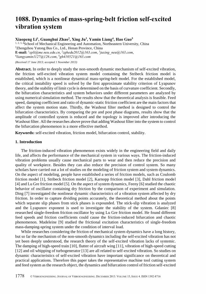
So a simple model is needed to make deep study. Considering systematic changes have direct
relationships with the mass, stiffness, damping, friction coefficient and normal vibration, the
mass-spring-belt self-excited vibration system model is established in Figure 1.
Drived part
m
Equivalent stiffness k
Equivalent damping c
Friction F
Normal force F0
Normal force tF sin1
Feed speed v
Fig. 1. The mechanical model of the mass-spring-belt system
The dynamic equation of the system is:
𝑚𝑑2𝑥
𝑑𝑡2+ 𝑐
𝑑𝑥
𝑑𝑡+ 𝑘𝑥 − 𝐹 = 0. (1)
Then the dimensionless expression is:
�̈� + 2𝛽�̇� + 𝑋 − 𝜇 = 0, (2)
where 𝐹 = 𝑁𝜇, 𝜔0 = √𝑘 𝑚⁄ , 𝜏 = 𝜔0𝑡, 𝑋 = 𝑥𝑘/𝑁, 2𝛽 = 𝑐𝜔/𝑘, 𝑣0 =𝑣0
𝜔0𝐿, 𝛺 =
�̃�
𝜔0.
The Stribeck friction model is introduced in this paper. This model is very classical and can
describe the general friction behavior of joint surfaces of mechanical movement of parts. The
expression of the model is:
𝜇 = −𝜇𝑠𝑠𝑔𝑛 (𝑑𝑋
𝑑𝜏− 𝑣0) +
3(𝜇𝑠 − 𝜇𝑚)
2𝑣𝑚(𝑑𝑋
𝑑𝜏− 𝑣0) −
(𝜇𝑠 − 𝜇𝑚)
2𝑣𝑚3
(𝑑𝑋
𝑑𝜏− 𝑣0)
3
, (3)
where �̇� = 𝑑𝑋/𝑑𝜏 is the non-dimensional speed, 𝜈0 is the belt speed, 𝑣𝑚 is the speed that

1088. DYNAMICS OF MASS-SPRING-BELT FRICTION SELF-EXCITED VIBRATION SYSTEM.
XIAOPENG LI, GUANGHUI ZHAO, XING JU, YAMIN LIANG, HAO GUO
1780 © VIBROENGINEERING. JOURNAL OF VIBROENGINEERING. DECEMBER 2013. VOLUME 15, ISSUE 4. ISSN 1392-8716
corresponds to the minimum dynamic friction, 𝜇𝑠 is dynamic friction coefficient, 𝜇𝑚 is the static
friction coefficient.
Based on the theory of ordinary differential equations, the higher order differential equation
can be transformed into first order differential equations. The equivalent transformation is made
as:
{
𝑋 = 𝑋1,𝑑𝑋
𝑑𝜏= 𝑋2.
(4)
Then the Equation (3) can be transformed into first order differential equations:
{
𝑑𝑋1
𝑑𝜏= 𝑋2,
𝑑𝑋2𝑑𝜏
= −2𝛽𝑋2 − 𝑋1 − 𝜇𝑠sgn (𝑑𝑋
𝑑𝜏− 𝑣0) +
3(𝜇𝑠 − 𝜇𝑚)
2𝑣𝑚(𝑑𝑋
𝑑𝜏− 𝑣0) −
𝜇𝑠 − 𝜇𝑚2𝑣𝑚
3(𝑑𝑋
𝑑𝜏− 𝑣0)
3
.
(5)
Based on the reference [14], when the input speed of the system is very fast, the mass block is
in the condition of static balance under the effect of friction force and spring force. In this
condition �̈� = 0, �̇� = 0, sgn(𝑣𝑟) = –1. When 𝜇𝑠 = 0.4, 𝜇𝑚 = 0.25, 𝑣𝑚 = 0.5, the stability of
balance point can be analysed by Lyapunov stability theory.
When 𝑑𝑋𝑖
𝑑𝜏= 0 in Equation (5), the equilibrium point of the system is solved as:
{𝑋20 = 0,
𝑋10 = 𝜇 = 0.4 − 0.45𝑣0 + 0.6𝑣03 ,
(6)
where {𝑋1 = �̅�1 + 𝑋10,
𝑋2 = �̅�2 + 𝑋20, {𝐹1 = 0,
𝐹2 = −0.45�̅�2 + 0.6(�̅�23 + 3�̅�2𝑣𝑟
2 − 3�̅�22).
The first approximate equation is obtained after expanding the Equation (5) into Taylor series
and dropping the quadratic term. For the first approximate equation, the jacobian matrix of
variables 𝑋1 and 𝑋2 can be expressed as Equation (7) when 𝑋1 = 0 and 𝑋2 = 0:
𝐴 = [0 1𝑎21 𝑎22
] = 0. (7)
When dimensionless damping coefficient 𝛽 = 0.01, the characteristic equation of matrix 𝐴 is:
|𝜆𝐸 − 𝐴| = |𝜆 1−1 𝜆 − (0.45 − 𝛽 − 1.8𝑣0
2)| = 𝜆2 − (0.44 − 1.8𝑣0
2)𝜆 + 1 = 0. (8)
For the certain driving velocity 𝑣0, the equilibrium point and its corresponding eigenvalue can
be obtained by the Equation (6) and Equation (8). Based on the Hurwits law, the critical instability
speed of system can be solved by 𝑝 = 0.44 − 1.8𝑣02 = 0. In this condition 𝑣𝑏1 = 0.4944 is the
supercritical Hopf bifurcation point.
The amplitude approximate solution of limit cycle in multi-dimensional system has pointed
that curvature coefficient is an important basis to determine the stability of limit cycle. Regarding
the Hopf bifurcation characteristics as the starting point, this paper gets the Jordan standard form
by proper linear transform and deduces the expression of curvature coefficient of limit cycle by
centre manifold theory [14]. So in order to judge the stability of limit cycle, the linear
transformation is taken into the standard form in Equation (5):
1088. DYNAMICS OF MASS-SPRING-BELT FRICTION SELF-EXCITED VIBRATION SYSTEM.
XIAOPENG LI, GUANGHUI ZHAO, XING JU, YAMIN LIANG, HAO GUO
© VIBROENGINEERING. JOURNAL OF VIBROENGINEERING. DECEMBER 2013. VOLUME 15, ISSUE 4. ISSN 1392-8716 1781
�̇� = 𝐴𝑌 + 𝑄, (9)
where 𝐴 = [0 1−1 0.44 − 1.8𝑣0
2], 𝑄 = {𝑄1,𝑄2,
= {0,
1.8𝑣0𝑦22 − 0.6𝑦2
3.
Based on the Equation (6), the equilibrium point is (𝑦, �̇�) = (0,0.4 − 0.45𝑣0 + 0.6𝑣03). And
the eigenvalues of Equation (7) are:
𝜆1,2 = 𝛼(𝑣0) ± 𝛽(𝑣0), (10)
where 𝛼(𝑣0) = (0.44 − 1.8𝑣02)/2, 𝛽(𝑣0) = √(0.44 − 1.8𝑣0
2)2 − 4/2.
When 𝛼(𝑣0) = (0.44 − 1.8𝑣02)/2 = 0:
𝛼′(0) = ((0.44 − 1.8𝑣02) 2⁄ )′|𝑣0=𝑣𝑏1 = −3.6 × 0.4944 = −1.7798 < 0, (11)
𝑔20 =1
4(𝜕2𝑄1
𝜕𝑦12 −
𝜕2𝑄1
𝜕𝑦22 + 2
𝜕2𝑄1𝜕𝑦1𝜕𝑦2
+ 𝑖 (𝜕2𝑄2
𝜕𝑦12 −
𝜕2𝑄2
𝜕𝑦22 − 2
𝜕2𝑄1𝜕𝑦1𝜕𝑦2
)) = −1.7788
4𝑖, (12)
𝑔11 =1
4(𝜕2𝑄1
𝜕𝑦12 +
𝜕2𝑄1
𝜕𝑦22 + 𝑖 (
𝜕2𝑄2
𝜕𝑦12 +
𝜕2𝑄2
𝜕𝑦22 )) =
1.7788
4𝑖, (13)
𝐺21 =1
8(𝜕3𝑄1
𝜕𝑦13 +
𝜕3𝑄1
𝜕𝑦1𝜕𝑦22 +
𝜕3𝑄2
𝜕𝑦12𝜕𝑦2
+𝜕3𝑄2
𝜕𝑦23 + 𝑖 (
𝜕3𝑄2
𝜕𝑦13 −
𝜕3𝑄2
𝜕𝑦1𝜕𝑦22 − 2
𝜕3𝑄1
𝜕𝑦12𝜕𝑦2
))
= −3.6
8.
(14)
Based on the Equation (12), Equation (13) and Equation (14), the curvature coefficient of limit
cycle is:
𝜎1 = Re {𝑔20𝑔112𝜔0
} Re {−3.6
16+1.77882
16𝑖} = −
3.6
16< 0. (15)
When 𝜎1 < 0 and 𝛼′(0) < 0, the bifurcation of system is generated in the point of 𝑣 = 𝑣𝑏1.
In the direction of 𝑣 < 𝑣𝑏1 the limit cycle is in a stable status, while the equilibrium point is in an
unstable state.
When the feed speed 𝑣0 = 0.45 < 𝑣𝑏1, the criterion conditions of stability are: 𝛥 = 𝑝2 − 4𝑞 < 0, 𝑝 > 0. Then the eigenvalues of the equation do not have negative real parts.
The equilibrium point is an unstable focus and produces the limit cycle which tends to be stable.
So the ultimate motion is periodic motion and can be divided into two types: the pure sliding
vibration where the stick-slip vibration of the mass block never occurred and the stick-slip
vibration where the mass block is viscous on the belt on occasion.
When the feed speed 𝑣0 = 0.495 > 𝑣𝑏1, the criterion conditions of stability are:
𝛥 = 𝑝2 − 4𝑞 < 0, 𝑝 < 0. Then the eigenvalues of the equation have negative real parts. The
equilibrium point is a stable focus and the solution of equation is gradually attenuating to zero. So
the ultimate motion is stable.
3. Numerical simulation of friction self-excited vibration system
3.1. Bifurcation numerical simulation
Hopf bifurcation is that the equilibrium point changes from stable focus into unstable focus
when the parameters pass by the critical point. It is an important dynamic bifurcation problem and
has a close relation with the generation of self-excited vibration in engineering.
1088. DYNAMICS OF MASS-SPRING-BELT FRICTION SELF-EXCITED VIBRATION SYSTEM.
XIAOPENG LI, GUANGHUI ZHAO, XING JU, YAMIN LIANG, HAO GUO
1782 © VIBROENGINEERING. JOURNAL OF VIBROENGINEERING. DECEMBER 2013. VOLUME 15, ISSUE 4. ISSN 1392-8716
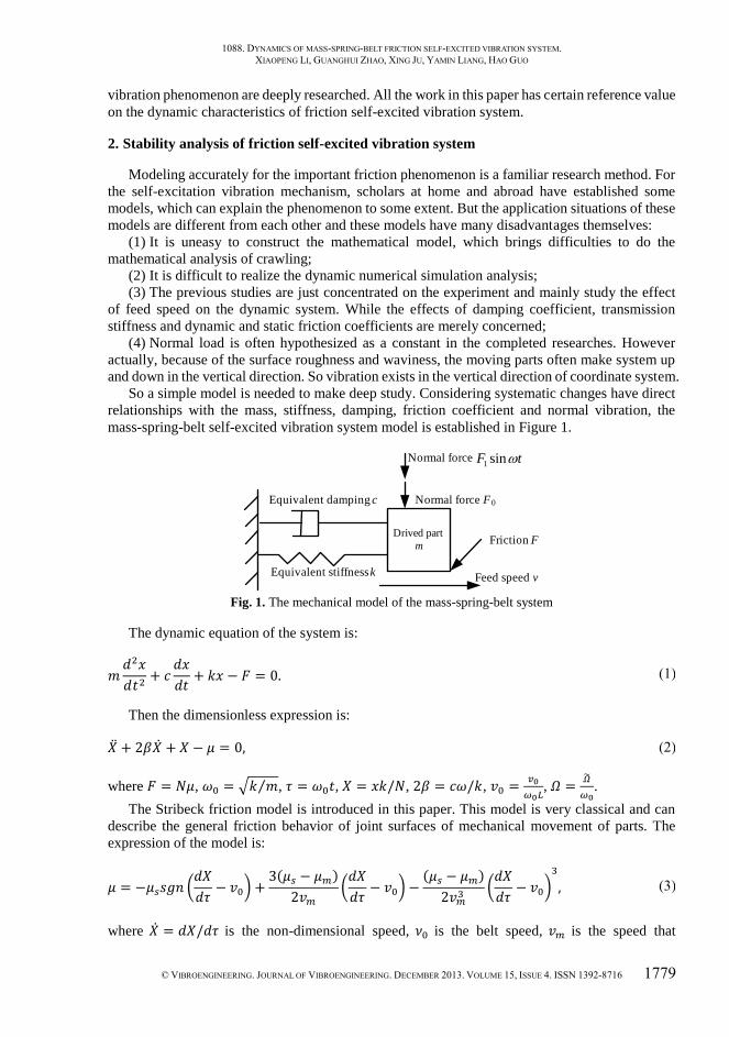
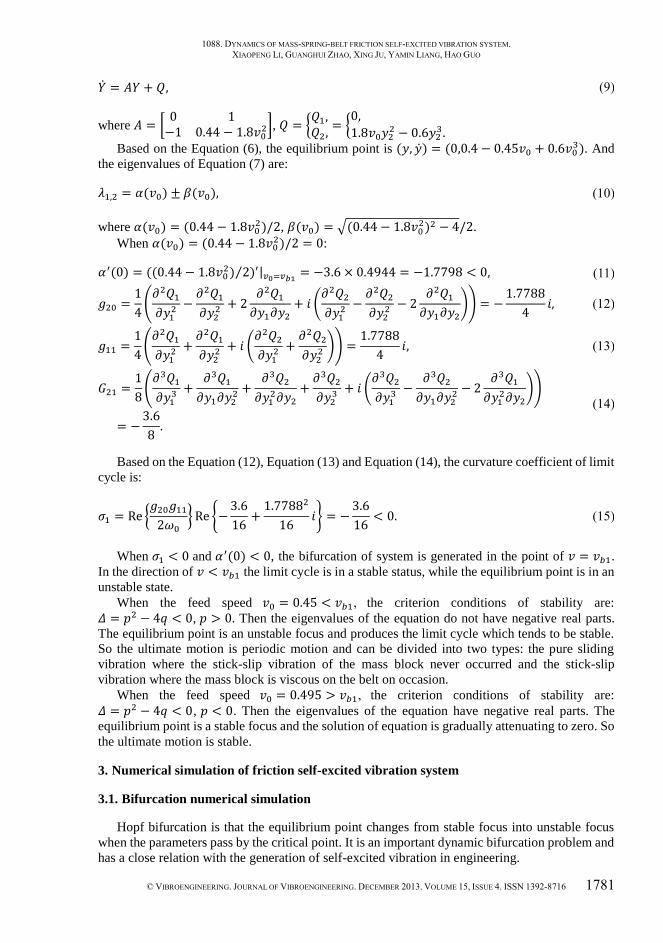
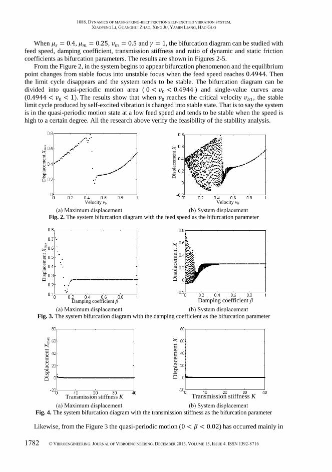
When 𝜇𝑠 = 0.4, 𝜇𝑚 = 0.25, 𝑣𝑚 = 0.5 and 𝛾 = 1, the bifurcation diagram can be studied with
feed speed, damping coefficient, transmission stiffness and ratio of dynamic and static friction
coefficients as bifurcation parameters. The results are shown in Figures 2-5.
From the Figure 2, in the system begins to appear bifurcation phenomenon and the equilibrium
point changes from stable focus into unstable focus when the feed speed reaches 0.4944. Then
the limit cycle disappears and the system tends to be stable. The bifurcation diagram can be
divided into quasi-periodic motion area ( 0 < 𝑣0 < 0.4944 ) and single-value curves area
(0.4944 < 𝑣0 < 1). The results show that when 𝑣0 reaches the critical velocity 𝑣𝑏1, the stable
limit cycle produced by self-excited vibration is changed into stable state. That is to say the system
is in the quasi-periodic motion state at a low feed speed and tends to be stable when the speed is
high to a certain degree. All the research above verify the feasibility of the stability analysis.
Velocity v0
Dis
pla
cem
ent
Xm
ax
(a) Maximum displacement
Velocity v0
Dis
pla
cem
ent
X
(b) System displacement
Fig. 2. The system bifurcation diagram with the feed speed as the bifurcation parameter
Damping coefficient β
Dis
pla
cem
ent
Xm
ax
(a) Maximum displacement
Damping coefficient β
Dis
pla
cem
ent
X
(b) System displacement
Fig. 3. The system bifurcation diagram with the damping coefficient as the bifurcation parameter
Transmission stiffness K
Dis
pla
cem
ent
Xm
ax
(a) Maximum displacement
Transmission stiffness K
Dis
pla
cem
ent
X
(b) System displacement
Fig. 4. The system bifurcation diagram with the transmission stiffness as the bifurcation parameter
Likewise, from the Figure 3 the quasi-periodic motion (0 < 𝛽 < 0.02) has occurred mainly in

1088. DYNAMICS OF MASS-SPRING-BELT FRICTION SELF-EXCITED VIBRATION SYSTEM.
XIAOPENG LI, GUANGHUI ZHAO, XING JU, YAMIN LIANG, HAO GUO
© VIBROENGINEERING. JOURNAL OF VIBROENGINEERING. DECEMBER 2013. VOLUME 15, ISSUE 4. ISSN 1392-8716 1783
small damping coefficient region. The system will be stable when the damping coefficient is high
to a certain degree. From the Figure 4 the influence of transmission stiffness on the system
characteristics is not so great. Only increasing transmission stiffness will not inhibit the
self-excited vibration. From the Figure 5 larger ratio of dynamic and static friction coefficients
leads to the phenomenon of self-excited vibration. Inversely, the stable state occurs in a small ratio
of dynamic and static friction coefficients.
Static-dynamic friction
coefficient μm/μs
Dis
pla
cem
ent
Xm
ax
(a) Maximum displacement
Static-dynamic friction
coefficient μm/μs
Dis
pla
cem
ent
X
(b) System displacement
Fig. 5. The system bifurcation diagram with the ratio of dynamic and
static friction coefficients as the bifurcation parameter
3.2. Numerical simulation under different feed speeds
When 𝛽 = 0.01, 𝜇𝑠 = 0.4, 𝜇𝑚 = 0.25, 𝑣𝑚 = 0.5, 𝛾 = 1 and the initial conditions are 𝑋 = 0,
�̇� = 0, the phase diagrams under different feed speeds are shown in Figure 6, where 𝑣𝑏1 = 0.4944, 𝑣𝑏0 = 0.4372.
Displacement X
Vel
oci
ty d
X/dτ
(a) 𝑣0 = 0.75 > 𝑣𝑏1
Displacement X
Vel
oci
ty d
X/dτ
(b) 𝑣0 = 0.55 > 𝑣𝑏1
Displacement X
Vel
oci
ty d
X/dτ
(c) 𝑣0 = 0.49 ∈ [𝑣𝑏0, 𝑣𝑏1]
Displacement X
Vel
oci
ty d
X/dτ
(d) 𝑣0 = 0.45 ∈ [𝑣𝑏0, 𝑣𝑏1]
Displacement X
Vel
oci
ty d
X/dτ
(e) 𝑣0 = 0.43 < 𝑣𝑏0
Displacement X
Vel
oci
ty d
X/dτ
(f) 𝑣0 = 0.35 < 𝑣𝑏0
Fig. 6. The phase diagrams under the action of different feed speeds
From the Figure 6, system motion can be divided into three stages when feed speed changes
between critical velocities. When the feed speed is 𝑣0 > 𝑣𝑏1 = 0.4944 , the system will be
stabilized at the equilibrium point. Then the relative velocity is the feed speed. The time tending
to be stable decreased with the feed speed increased. That is to say, the bigger the feed speed the
better stability it has. In the equilibrium point of system occurs instability and it begins to cause
1088. DYNAMICS OF MASS-SPRING-BELT FRICTION SELF-EXCITED VIBRATION SYSTEM.
XIAOPENG LI, GUANGHUI ZHAO, XING JU, YAMIN LIANG, HAO GUO
1784 © VIBROENGINEERING. JOURNAL OF VIBROENGINEERING. DECEMBER 2013. VOLUME 15, ISSUE 4. ISSN 1392-8716
self-excited vibration when the feed speed is 𝑣0 < 𝑣𝑏1. The process can be further divided into
pure slip (𝑣𝑏0 < 𝑣0 < 𝑣𝑏1) where in the phase diagram does not exist limit cycle and the minimum
relative speed between mass block and belt is not zero, and stick slip (𝑣0 < 𝑣𝑏0 = 0.4372) where
the limit cycle has obvious viscous stage and the minimum relative speed between mass block and
belt is zero. When the minimum relative speed is zero, the input speed is the demarcation point
translated from pure slip into stick slip.
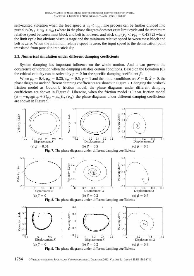
3.3. Numerical simulation under different damping coefficients
System damping has important influence on the whole motion. And it can prevent the
occurrence of vibration when the damping satisfies certain conditions. Based on the Equation (8),
the critical velocity can be solved by 𝑝 = 0 for the specific damping coefficient 𝛽.
When 𝜇𝑠 = 0.4, 𝜇𝑚 = 0.25, 𝑣𝑚 = 0.5, 𝛾 = 1 and the initial conditions are 𝑋 = 0, �̇� = 0, the
phase diagrams under different damping coefficients are shown in Figure 7. Changing the Stribeck
friction model as Coulomb friction model, the phase diagrams under different damping
coefficients are shown in Figure 8. Likewise, when the friction model is linear friction model
(𝜇 = −𝜇𝑠sgn𝑣𝑟 + 3(𝜇𝑠 − 𝜇𝑚)𝑣𝑟/𝑣𝑚), the phase diagrams under different damping coefficients
are shown in Figure 9.
Displacement X
Vel
oci
ty d
X/dτ
(a) 𝛽 = 0.01
Displacement X
Velo
cit
y d
X/dτ
(b) 𝛽 = 0.5
Displacement X
Vel
oci
ty d
X/dτ
(c) 𝛽 = 0.5
Fig. 7. The phase diagrams under different damping coefficients
Displacement X
Vel
oci
ty d
X/dτ
(a) 𝛽 = 0
Displacement X
Vel
oci
ty d
X/dτ
(b) 𝛽 = 0.2
Displacement X
Vel
oci
ty d
X/dτ
(c) 𝛽 = 0.8
Fig. 8. The phase diagrams under different damping coefficients
Displacement X
Vel
oci
ty d
X/dτ
(a) 𝛽 = 0
Displacement X
Vel
oci
ty d
X/dτ
(b) 𝛽 = 0.2
Displacement X
Vel
oci
ty d
X/dτ
(c) 𝛽 = 0.8
Fig. 9. The phase diagrams under different damping coefficients

1088. DYNAMICS OF MASS-SPRING-BELT FRICTION SELF-EXCITED VIBRATION SYSTEM.
XIAOPENG LI, GUANGHUI ZHAO, XING JU, YAMIN LIANG, HAO GUO
© VIBROENGINEERING. JOURNAL OF VIBROENGINEERING. DECEMBER 2013. VOLUME 15, ISSUE 4. ISSN 1392-8716 1785
From the Figure 7, the proportion of viscous stage decreased with the increase of damping.
When the damping is great to a certain degree, the viscous stage disappears and the system begins
stable pure slip motion. Continuing increase of the damping to the critical value, the system will
be stable at the equilibrium point. So increasing damping to a certain extent can inhibit the
self-excited vibration and improve the stability of the system. Comparing the Figure 8 with
Figure 9, when the friction model is linear friction model where the relationship between friction
and speed is with negative slope, self-induced vibration occurs in the system. And the proportion
of viscous stage decreased with the increase of damping. The results show that negative friction-
speed slope is the main cause of self-induced vibration.
3.4. Numerical simulation under different transmission stiffness
Transmission stiffness has important influence on the whole motion. Based on the stability
theoretical analysis above, transmission stiffness has the function of improving the stability of
system. When 𝜇𝑠 = 0.4, 𝜇𝑚 = 0.25, 𝑣𝑚 = 0.5, 𝛾 = 1, 𝛽 = 0.01, 𝑣0 = 0.2 and the initial
conditions are 𝑋 = 0, �̇� = 0, the phase diagrams under different transmission stiffnesses are
shown in Figure 10.
Displacement X
Vel
oci
ty d
X/dτ
(a) 𝐾 = 1
Displacement X
Vel
oci
ty d
X/dτ
(b) 𝐾 = 2
Displacement XV
elo
city
dX
/dτ
(c) 𝐾 = 4
Displacement X
Vel
oci
ty d
X/dτ
(d) 𝐾 = 20
Displacement X
Vel
oci
ty d
X/dτ
(e) 𝐾 = 100
Displacement X
Vel
oci
ty d
X/dτ
(f) 𝐾 = 300
Fig. 10. The phase diagrams under different transmission stiffnesses
From the Figure 10, the proportion of viscous stage decreased with the increase of transmission
stiffness. When the transmission stiffness is great to a certain degree, the viscous stage disappears
and the system begins stable pure slip motion. And the limit cycle decreased with the increase of
stiffness. So increasing stiffness to a certain extent can shorten viscous stage and improve the
stability of the system.
3.5. Numerical simulation under different dynamic and static friction coefficients
When 𝛽 = 0.01, 𝜇𝑠 = 0.4, 𝜇𝑚 = 0.25, 𝑣𝑚 = 0.5, 𝛾 = 1 and the initial conditions are 𝑋 = 0,
�̇� = 0, the phase diagrams under different dynamic and static friction coefficients are shown in
Figure 11.
From the Figure 11, vibration amplitude of the system and the proportion of viscous stage
increased with the increase of gap of dynamic and static friction coefficients. When the gap of
dynamic and static friction coefficients is decreased to a certain degree, the viscous stage

1088. DYNAMICS OF MASS-SPRING-BELT FRICTION SELF-EXCITED VIBRATION SYSTEM.
XIAOPENG LI, GUANGHUI ZHAO, XING JU, YAMIN LIANG, HAO GUO
1786 © VIBROENGINEERING. JOURNAL OF VIBROENGINEERING. DECEMBER 2013. VOLUME 15, ISSUE 4. ISSN 1392-8716
disappears and the system begins stable pure slip motion. Continuing decrease of the gap, the
system will be stable and no longer performing vibration.
Displacement X
Vel
oci
ty d
X/dτ
(a) 𝜇𝑠 = 0.4, 𝜇𝑐 = 0.2
Displacement XV
elo
city
dX
/dτ
(b) 𝜇𝑠 = 0.4, 𝜇𝑐 = 0.25
Displacement X
Vel
oci
ty d
X/dτ
(c) 𝜇𝑠 = 0.4, 𝜇𝑐 = 0.3
Displacement X
Vel
oci
ty d
X/dτ
(d) 𝜇𝑠 = 0.4, 𝜇𝑐 = 0.35
Displacement X
Vel
oci
ty d
X/dτ
(e) 𝜇𝑠 = 0.4, 𝜇𝑐 = 0.38
Displacement X
Vel
oci
ty d
X/dτ
(f) 𝜇𝑠 = 0.4, 𝜇𝑐 = 0.39
Fig. 11. The phase diagrams under the difference of dynamic and static friction coefficients
4. Bifurcation control of friction self-excited vibration system
4.1. Design of Washout filter and the stability analysis
When the feed speed is 0.48, 0.49 and 0.492, the dynamic characteristics of friction self-excited
vibration can be obtained and the phase diagrams are shown in Figure 12.
Displacement X
Vel
oci
ty d
X/dτ
(a) 𝑣0 = 0.48 ∈ [𝑣𝑏0, 𝑣𝑏1]
Displacement X
Vel
oci
ty d
X/dτ
(b) 𝑣0 = 0.49 ∈ [𝑣𝑏0, 𝑣𝑏1]
Displacement X
Vel
oci
ty d
X/dτ
(c) 𝑣0 = 0.492 ∈ [𝑣𝑏0, 𝑣𝑏1]
Fig. 12. The phase diagrams under the action of different feed speeds
From the Figure 12, when the feed speed is greater than or equal to 0.49, amplitude of the limit
cycle becomes suddenly decreased and the equilibrium point is in an unstable state. In the process
of decreasing the feed speed, the limit cycle changed from stable into unstable and the equilibrium
point changed from unstable into stable. Based on the stability analysis, in the system occurs the
subcritical bifurcation when speed passes by the point of 0.49. To decrease the amplitude,
Washout filter is introduced to control the bifurcation [15].
When the friction is linear, the friction self-excited vibration system can be expressed as:
{�̇� = 𝑦,�̇� = −𝐹 − 𝐶𝑦 − 𝐾𝑥,
(16)
where 𝐹 = −0.45�̅�2 + 0.6(�̅�23 + 3�̅�2𝑣𝑟
2 − 3�̅�22).

1088. DYNAMICS OF MASS-SPRING-BELT FRICTION SELF-EXCITED VIBRATION SYSTEM.
XIAOPENG LI, GUANGHUI ZHAO, XING JU, YAMIN LIANG, HAO GUO
© VIBROENGINEERING. JOURNAL OF VIBROENGINEERING. DECEMBER 2013. VOLUME 15, ISSUE 4. ISSN 1392-8716 1787
To control 𝑦 with Washout filter, the control system can be expressed as:
{
�̇� = 𝑦,�̇� = −𝐹 − 𝐶𝑦 − 𝐾𝑥,�̇� = 𝑦 − 𝑑𝜔.
(17)
The controller can be designed as the form of:
𝑢 = 𝑔(𝑣; 𝐾) = 𝑘1𝑣 + 𝑘2𝑣3, (18)
where 𝐾 = (𝑘1, 𝑘2) is the control vector, 𝑘1 is the linear gain, 𝑘2 is non-linear gain. The linear
part can control the production of Hopf bifurcation, the cubic term can control the amplitude of
the limit cycle.
Taking Equation (17) into Equation (18), the system can be expressed as Equation (19):
{
�̇� = 𝑦,
�̇� = −𝐹 − 𝐶𝑦 − 𝐾𝑥 + 𝑘1(𝑦 − 𝑑𝜔) + 𝑘2(𝑦 − 𝑑𝜔)3,
�̇� = 𝑦 − 𝑑𝜔. (19)
The Jacobian matrix of the linear part of the system is:
𝐽 = [0 1 0−1 0.0078 + 𝑘1 −2𝑘10 1 −2
]. (20)
The characteristic equation of the Jacobian matrix is:
𝜆3 + 𝑐1𝜆2 + 𝑐2𝜆 + 𝑐3 = 0, (21)
where 𝑐1 = 2 − (0.44 − 1.8𝑣02 + 𝑘1), 𝑐2 = 2𝑘1 − (0.44 − 1.8𝑣0
2 + 1), 𝑐3 = 2.
Based on the Routh-Hurwits criterion 𝑐1𝑐2 = 𝑐3, that is to say 𝑘1 = −0.0395 is the condition
of Hopf bifurcation. The amplitude of limit cycle can be regulated by changing the value of 𝑘2.
The characteristic roots of Equation (21) are 𝜆1,2 = 𝛼(𝑣0) ± 𝛽(𝑣0) and 𝜆3 = 𝑐, where
𝛼(𝑣0) = −(1.5995 + 1.8𝑣02) + 𝛰(𝑣0
2) and:
𝛼′(0) = (−(1.5995 + 1.8𝑣02))
′|𝑣0=0.49
= −3.6 × 0.49 = −1.764 < 0. (22)
When 𝑣0 = 0.49, the characteristic quantities are:
𝑔20 =1
4(𝜕2𝑄1
𝜕𝑦12 −
𝜕2𝑄1
𝜕𝑦22 + 2
𝜕2𝑄1𝜕𝑦1𝜕𝑦2
+ 𝑖 (𝜕2𝑄2
𝜕𝑦12 −
𝜕2𝑄2
𝜕𝑦22 − 2
𝜕2𝑄1𝜕𝑦1𝜕𝑦2
)) = −1.764
4𝑖, (23)
𝑔11 =1
4(𝜕2𝑄1
𝜕𝑦12 +
𝜕2𝑄1
𝜕𝑦22 + 𝑖 (
𝜕2𝑄2
𝜕𝑦12 +
𝜕2𝑄2
𝜕𝑦22 )) =
1.764
4𝑖, (24)
𝐺110 =1
2(𝜕2𝑄1𝜕𝑦1𝜕𝑦3
+𝜕2𝑄2𝜕𝑦1𝜕𝑦3
+ 𝑖 (𝜕2𝑄2𝜕𝑦1𝜕𝑦3
−𝜕2𝑄1𝜕𝑦1𝜕𝑦3
)) = 0, (25)
𝐺101 =1
2(𝜕2𝑄1𝜕𝑦1𝜕𝑦3
−𝜕2𝑄2𝜕𝑦1𝜕𝑦3
+ 𝑖 (𝜕2𝑄2𝜕𝑦1𝜕𝑦3
+𝜕2𝑄1𝜕𝑦1𝜕𝑦3
)) = 0, (26)

1088. DYNAMICS OF MASS-SPRING-BELT FRICTION SELF-EXCITED VIBRATION SYSTEM.
XIAOPENG LI, GUANGHUI ZHAO, XING JU, YAMIN LIANG, HAO GUO
1788 © VIBROENGINEERING. JOURNAL OF VIBROENGINEERING. DECEMBER 2013. VOLUME 15, ISSUE 4. ISSN 1392-8716
𝑤20 =1
4 (2𝑖𝜔(𝜇0 − 𝜆3(𝜇0)))(𝜕2𝑄3
𝜕𝑦12 −
𝜕2𝑄3
𝜕𝑦22 − 2𝑖
𝜕2𝑄3𝜕𝑦1𝜕𝑦3
) = 0, (27)
𝑤11 =1
4𝜆3(𝜇0)(𝜕2𝑄3
𝜕𝑦12 +
𝜕2𝑄3
𝜕𝑦22 ) = 0, (28)
𝐺21 =1
8(𝜕3𝑄2
𝜕𝑦23 ) =
1
8(6𝑘3 − 3.6). (29)
According to the Equation (23) to Equation (29), the curvature coefficient of limit cycle is:
𝜎1 = Re {𝑔20𝑔112𝜔0
+𝐺21 + 𝐺101𝑔20
2} = Re {
1
8(6𝑘3 − 3.6) +
3.62
16𝑖} =
1
8(6𝑘3 − 3.6). (30)
It can be seen obviously 𝜎1 < 0 when 𝑘3 < 0.6 . Based on 𝜎1 < 0 and 𝛼′(0) < 0 , in the
system will occur Hopf bifurcation at the point of 𝑣 = 0.49 and the bifurcation direction is
𝑣 < 0.49.
4.2. Simulation analysis verification of bifurcation control
Before introducing the Washout filter, the Hopf supercritical bifurcation happens in the
equilibrium point. Based on the bifurcation diagram with feed speed as the bifurcation parameter
given above, the amplitude of the system changes remarkably and increases suddenly when the
feed speed reduces approximately to 0.49. That is to say the subcritical bifurcation has happened.
After introducing the Washout filter, the Hopf supercritical bifurcation still happens in the
equilibrium point. But the amplitude of system decreases when 𝑣0 = 0.49 . This shows that
subcritical bifurcation is controlled.
When 𝑣0 = 0.4 , the phase diagrams are obtained after introducing the Washout filter at
different values of 𝑘1 and 𝑘2, they are shown in Figure 13.
Displacement X
Vel
oci
ty d
X/dτ
(a) 𝑘1 = −0.0395, 𝑘2 = −0.01
Displacement X
Vel
oci
ty d
X/dτ
(b) 𝑘1 = −0.0395, 𝑘2 = −0.4
Displacement X
Vel
oci
ty d
X/dτ
(c) 𝑘1 = −0.0395, 𝑘2 = −0.8
Fig. 13. The phase diagrams of the controlled system at different parameters
From the Figure 13, adjusting the parameters of controller can change the amplitude of
self-induced vibration and make the limit cycle disappear. The Hopf bifurcation is well controlled.
The results show that the Washout filter control designed above is reasonable.
5. Conclusions
Based on the dynamic characteristics analysis of friction vibration structure, the friction self-
excited vibration system model containing the Stribeck model is established. For the certain feed
speed, the equilibrium point of the system is solved and the equilibrium stability is analyzed by
making use of the first approximate stability criterion of Lyapunov theory.
By the bifurcation numerical simulation and the numerical simulation under different
1088. DYNAMICS OF MASS-SPRING-BELT FRICTION SELF-EXCITED VIBRATION SYSTEM.
XIAOPENG LI, GUANGHUI ZHAO, XING JU, YAMIN LIANG, HAO GUO
© VIBROENGINEERING. JOURNAL OF VIBROENGINEERING. DECEMBER 2013. VOLUME 15, ISSUE 4. ISSN 1392-8716 1789
parameters of the system, stability analysis is verified feasible. The simulation results show that
great feed speed and damping coefficient and low gap of dynamic and static friction coefficients
can inhibit the self-excited variation to some extent. The research work of this paper has certain
reference value on the dynamics characteristics of the self-excited vibration system in actual
production.
The Washout filter method is introduced to control the Hopf bifurcation of friction self-excited
vibration. By comparing the pre and post phase diagrams, results show that the amplitude of
controlled system is reduced and the topology is improved after introducing the Washout filter.
So the Washout filter control is a comparatively effective method to control the bifurcation of
friction system.
Acknowledgement
This paper is supported by National Natural Science Foundation (51275079), Program for New
Century Excellent Talents in University (NCET-10-0301) and Fundamental Research Funds for
the Central Universities (N110403009).
References
[1] Den Hartog J. P. Forced vibration with combined Coulomb and viscous friction. Transactions of the
ASME, APM, Vol. 53, Issue 9, 1997, p. 107-115.
[2] Li Chun Bo, Pavelescu D. The friction-speed relation and its influence on the critical velocity of the
stick-slip motion. Wear, Vol. 82, Issue 3, 1982, p. 277-289.
[3] Karnopp D. Computer simulation of stick slip friction in mechanical dynamic systems. ASME Journal
of Dynamic Systems, Measurement and Control, Vol. 107, Issue 1, 1985, p. 100-103.
[4] Dahl P. R. Measurement of solid friction parameters of ball bearings. Proceedings of the 6th Annual
Symposium on Incremental Motion Control Systems and Devices, 1977, p. 49-60.
[5] Canudas De Wit C., Olsson H., Astrom K. J., Lischinsky P. A new model for control of systems
with friction. IEEE Transactions on Automatic Control, Vol. 40, Issue 3, 1995, p. 419-425.
[6] Feeny B., Moon F. C. Chaos in a forced dry-friction oscillator: experiments and numerical modeling.
Journal of Sound and Vibration, Vol. 170, Issue 3, 1994, p. 303-323.
[7] Wangcai Ding, Youqiang Zhang, Qingshuang Zhang Nonlinear dynamic analysis of vibrate system
with dry friction. Engineering Mechanics, Vol. 25, Issue 10, 2008, p. 212-217.
[8] Gdaniec P., Weiss C., Hoffmann N. P. On chaotic friction induced vibration due to rate dependent
friction. Mechanics Research Communications, Vol. 37, Issue 1, 2010, p. 92-95.
[9] Pascal M. New limit cycles of dry friction oscillators under harmonic load. Nonlinear Dynamics,
Vol. 70, Issue 2, 2012, p. 1435-1443.
[10] Caihong Huang Study on Vibration Reduction Technologies for High Speed Cars. Chengdu,
Southwest Jiaotong University, 2012.
[11] Fayou Yang, Zhongquan Gu Adaptive flutter suppression for aircraft wing. Journal of Nanjing
University of Aeronautics & Astronautics, Vol. 36, Issue 6, 2004, p. 708-712.
[12] Sinan Badrawy Cutting dynamics of high speed machining. WolfTracks, Vol. 81, 2001, p. 24-26.
[13] Kucherenko V. V., Gomez-Mancilla J. C. Bifurcations of an exactly solvable model of rotor
dynamics. International Journal of Bifurcation and Chaos in Applied Sciences and Engineering,
Vol. 10, Issue 12, 2000, p. 2689-2699.
[14] Suhua Liu Feedback Control of Hopf Bifurcation in Two Classes of Nonlinear High Dimensional
Systems. Changsha, Hunan University, 2008.
[15] Jun Ma, Gongliu Yang Bifurcation control of guideway stick-slip motion with Washout filter.
Transactions of Chinese Society of Agricultural Machinery, Vol. 39, Issue 11, 2008, p. 156-159.