11 cse 4705 artificial intelligence jinbo bi department of computer science & engineering jinbo
TRANSCRIPT

11
CSE 4705Artificial Intelligence
Jinbo BiDepartment of Computer Science & Engineering
http://www.engr.uconn.edu/~jinbo
2
Introduction and History
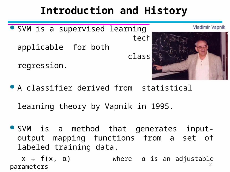
SVM is a supervised learning technique applicable for both classification and regression.
A classifier derived from statistical learning theory by Vapnik in 1995.
SVM is a method that generates input-output mapping functions from a set of labeled training data.
x → f(x, α) where α is an adjustable parameters
It is the simple geometrical interpretation of the margin, uniqueness of the solution, statistical robustness of the loss function, modularity of the kernel function, and overfit control through the choice of a single regularization parameter.

3
Advantage of SVM
Another name for regularization is The Capacity Control SVM controls the capacity by optimizing the classification margin.
– What is the margin?
– How can we optimize it?
– Linearly separable case
– Linearly inseparable case (using hinge loss)
– Primal-dual optimization
The other key features of SVMs are the use of kernels.
– What are the kernels? (May omit in this class)

4
Support Vector Machine
Find a linear hyperplane (decision boundary) that will separate the data

5
Support Vector Machine
One Possible Solution
B1

6
Support Vector Machine
Another Possible Solution
B2

7
Support Vector Machine
Other possible solutions
B2

8
Support Vector Machine
Which one is better? B1 or B2? How do you define better or the optimal?
B1
B2

9
Support Vector Machine Definitions
Examples closest to the hyperplane are support vectors.
B1
B2
b11
b12
b21
b22
margin
Support Vectors
Distance from a support vector to the separator is
Margin of the separator is the width of separation between support vectors of classes.
Basic concepts

10
Support Vector Machine
Find hyperplane that maximizes the margin So B1 is better than B2
B1
B2
b11
b12
b21
b22
margin
To find the optimal solution

11
Why Maximum Margin?
1. Intuitively this feels safest.
2. If we’ve made a small error in the location of the boundary (it’s been jolted in its perpendicular direction) this gives us least chance of causing a misclassification.
B1
B2
b11
b12
b21
b22
margin
3. The model is immune to removal of any non-support-vector data points.
4. There’s statistical learning theory (using VC dimension) that is related to (but not the same as) the proposition that this is a good thing.
5. Empirically it works very well.
12
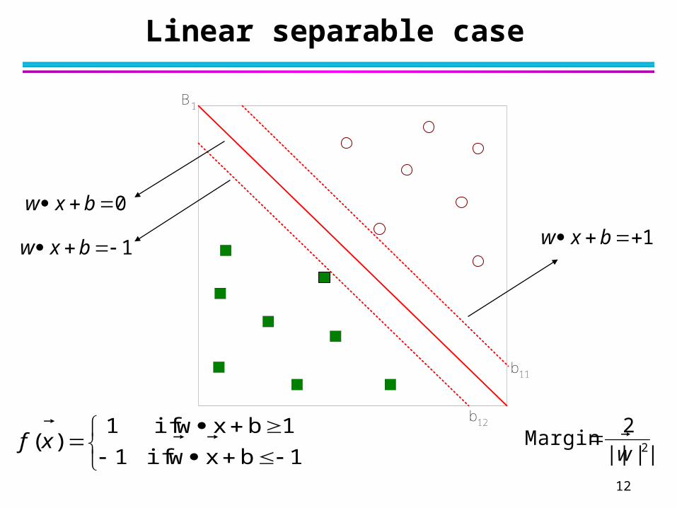
Linear separable case
B1
b11
b12
0 bxw
1 bxw 1 bxw
1bxw if1
1bxw if1)(
xf 2||||
2 Margin
w

13
Linear non-separable case (soft margin)
12
ii
ii
1bxw if1
-1bxw if1)(
ixf
Noisy data
Slack variables ξi
error

14
Nonlinear Support Vector Machines
What if the problem is not linearly separable?

15
Higher Dimensions
Mapping the data into higher dimensional space (kernel trick) where it is linearly separable and then we can use linear SVM – (easier to solve)
-1 0 +1
+ +-
(1,0)(0,0)
(0,1) +
+-

16
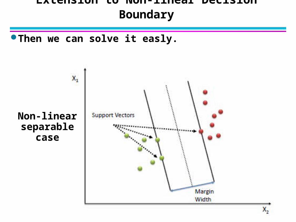
Extension to Non-linear Decision Boundary
Possible problem of the transformation– High computation overhead and hard to get a good estimate.
SVM solves these two issues simultaneously– Kernel tricks for efficient computation– Minimize ||w||2 can lead to a “good” classifier
Φ: x → φ(x)Non-linear separable case
17
Extension to Non-linear Decision Boundary
Then we can solve it easly.
Non-linear separable case

18
Non Linear non-separable case
What if decision boundary is not linear?
The concept of a kernel mapping function is very powerful. It allows SVM models to perform separations even with very complex boundaries

19
Linear Support Vector Machine
Find hyperplane that maximizes the margin So B1 is better than B2
B1
B2
b11
b12
b21
b22
margin

20
Definition
d1 = the shortest distance to the closest positive point
d2 = the shortest distance to the closest negative point
The margin of a separating hyperplane is d1 + d2.
Define the hyperplane H (decision function) such that:

21
Distance
Distance between Xn and the plane:- Take any point X on the plane- Projection of (Xn-) on W.
- = distance= |(Xn - | - distance= |Xn - |- = |Xn + b - - b|- = (if Xn is a support vector,
which makes Xn + b| =1)
Xn 𝑾 ¿
Xn
𝑾 ¿
𝑿 ¿¿ ¿
𝑿 ¿

22
SVM boundary and margin
Want: find W, b (offset) such that
subject to the constraint:
w
1Maximize
1||min N,...2,1n
bxw n
T
)(|| bb xwyxw n
T
nn
T 1)( bxwy n
T
n

23
The Lagrangian trick
We need to minimize Lp w.r.b to w,b and maximizing w.r.b >= 0
Reformulate the optimization problem:A ”trick” often used in optimization is to do an Lagrangian formulation of the problem.
The constraints will be replaced by constraints on the Lagrangian multipliers and the training data will only occur as dot products.

24
New formulation which is dependent on α , we need to maximize:
Having moved from minimizing LP to maximizing LD, we need to find:
This is a convex quadratic optimization problem, and we run a QP solver which will return alpha and then we can get w. What remains is to calculate b.
Dual form requires only the dot product of each input vector xi to be calculated

25
Definition of KKT conditions:
The Karush-Kuhn-Tucker Conditions
min ( )
. . h ( ) 0, 1, , ,
g ( ) 0, 1, , ,
j
k
n
f x
s t x j p
x k q
x X R
* *
* * *
1 1
*
1. ( ) 0, 1, , , ( ) 0, 1, , ,
2. ( ) ( ) ( ) 0,
0, 0, ( ) 0.
j k
p q
j j k kj k
j k k k
h x j p g x k q
f x h x g x
g x
The standard form of optimization is as follows:
The corresponding KKT conditions are:
Feasibility
Direction
( is the local minimum point)*x
26
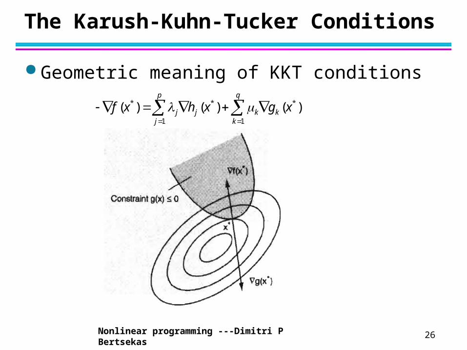
The Karush-Kuhn-Tucker Conditions
Geometric meaning of KKT conditions
* * *
1 1
( ) ( ) ( )p q
j j k kj k
f x h x g x
Nonlinear programming ---Dimitri P Bertsekas

27
The Karush-Kuhn-Tucker Conditions
Condition for KKT:
The intersection of the set of feasible directions with the set of descent directions coincides with the intersection of the set of feasible directions for linearized constraints with the set of descent directions
SVMs problems always satisfy this condition
Nonlinear programming ---Dimitri P Bertsekas

28
The Karush-Kuhn-Tucker Conditions
For the primal problem of linear SVMs,
0 1, ,
0
( ) 1 0 1,
0
( ( ) 1) 0
p v i i iviv
p i ii
i i
i
i i i
L y x v d
L yb
y x w b i l
i
y w x b i
The SVMs problem is convex( a convex objective function and convex feasible region), thus the KKT conditions are necessary and sufficient, which means the primal problem can be simplified to a KKT problem.
2
1 1
1( )
2
( ) 1 0 1,
0
l l
p i i i ii i
i i
i
L w y x w b
y x w b i l
i
The KKT conditions are:

29
Linearly Support Vector Machines
There are two cases of linearly Support Vector
Machines:
1- The Separable case.
2-The In-Separable case.

30
1- The Separable case:
Use it if there are no noises in training data.
0 bxw
1 bxw
1 bxw
hyperplane

31
If there are noises in training data.
We need to move
to the Non-
Separable case.

32
2-The In-Separable case:
Often, data will be noisy which does not allow any hyper-plane to
correctly classify all observations. Thus, the data are linearly
inseparable.
Idea: relax constraints using slack variables ξi in the constraints.
One for each sample.
Separable caseNon-Separable case

33
Slack variables
ξi is a measure of deviation from the ideal for xi.- ξi >1 : x is on the wrong side of the separating hyperplan.- 0 < ξi <1: x is correctly classified, but lies inside the margin.- ξi < 0 : x is correctly classified, and lies outside the margin.
Is the total distance of points on the wrong side of their margin
∑ ξ

34
To deal with the non-separable case, we can rewrite the
problem as:
minimize :
Subject to :
The parameter C controls the trarde-off between
maximizing the margin and minimizing the
training error.

35
Use the Lagrangian formulation for the optimization problem.
Introduce a positive Lagrangian multiplier for each inequality constraint.
Lagrangian multiplier
are the Lagrange multipliers introduced to enforce positivity of the error
is the weight coefficient
36
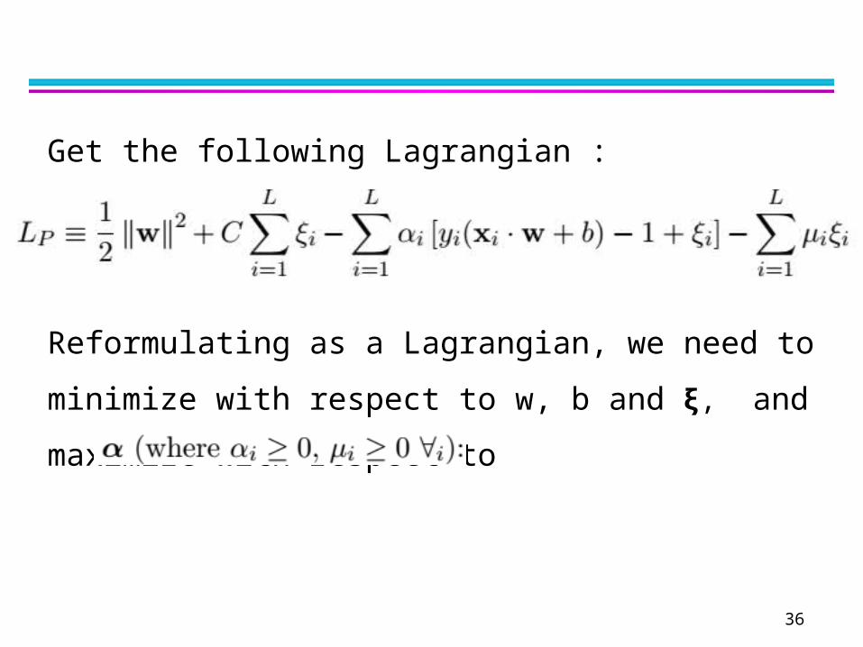
Get the following Lagrangian :
Reformulating as a Lagrangian, we need to minimize
with respect to w, b and ξ, and maximize with respect
to

37
Differentiating with respect to w, b and ξi and setting the derivatives to zero:
1
2

38
Substituting these 1, 2 into
We get a new formulation:

39
Calculate b
We run a QP solver which will return and from . will give us w. What remains is
to calculate b. Any data point satisfying (1) which is a Support
Vector xs will have the form: Substituting in (1), we will get :
Where S denotes the set of indices of the Support Vectors.
Faintly, we get this:
40
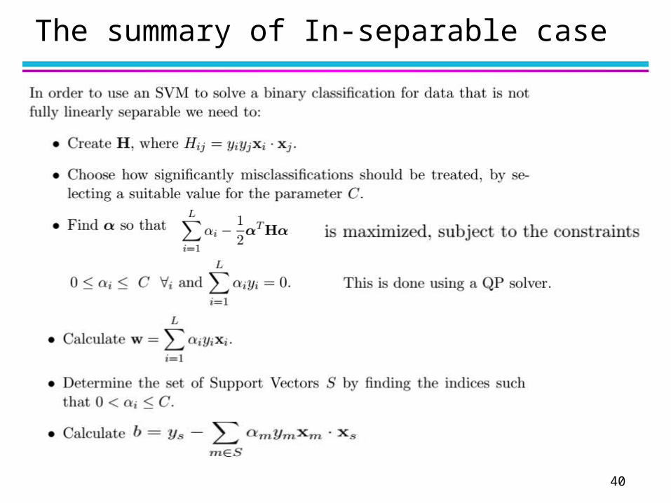
The summary of In-separable case

41
Non-linear SVMs
Cover’s theorem on the separability of patterns “A complex pattern-classification problem cast in a high-dimensional space non-linearly
is more likely to be linearly separable than in a low-dimensional space” The power of SVMs resides in the fact that they represent a robust and efficient
implementation of Cover’s theorem SVMs operate in two stages
Perform a non-linear mapping of the feature vector x onto a high-dimensional space that is hidden from the inputs or the outputs
Construct an optimal separating hyperplane in the high-dim space
42
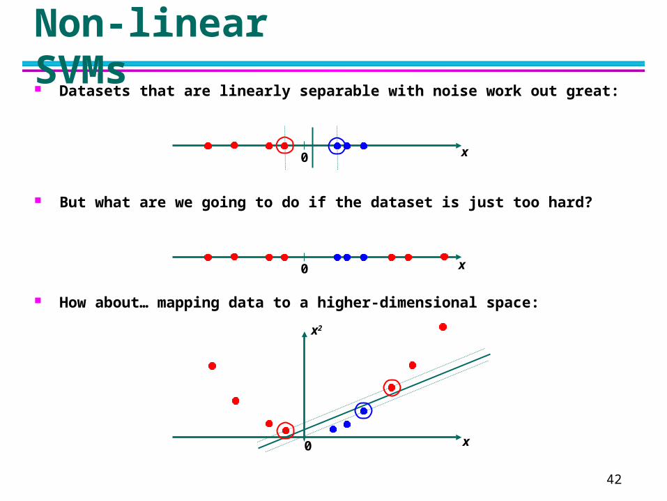
Non-linear SVMs Datasets that are linearly separable with noise work out great:
0 x
0 x
x2
0 x
But what are we going to do if the dataset is just too hard?
How about… mapping data to a higher-dimensional space:

43
Non-linear SVMs: Feature Space General idea: the original input space can be mapped to
some higher-dimensional feature space where the training set is separable:
Φ: x → φ(x)

44
Non-linear SVMs

45
Non-linear SVMs
Data is linearly separable in 3D This means that the problem can still be solved by a linear classifier

46
Non-linear SVMs
Naïve application of this concept by simply projecting to a high-dimensional non-linear manifold has two major problems Statistical: operation on high-dimensional spaces is ill-conditioned due to the “curse of
dimensionality” and the subsequent risk of overfitting –Computational: working in high-dim requires higher computational power, which poses limits on
the size of the problems that can be tackled
SVMs bypass these two problems in a robust and efficient manner First, generalization capabilities in the high-dimensional manifold are ensured by enforcing a
largest margin classifier
Recall that generalization in SVMs is strictly a function of the margin (or the VC dimension), regardless of the dimensionality of the feature space
Second, projection onto a high-dimensional manifold is only implicit
Recall that the SVM solution depends only on the dot product 𝑥𝑖,𝑥𝑗 between training examples
Therefore, operations in high-dim space ( ) do not have to be performed explicitly if we 𝜑 𝑥find a function (𝐾 𝑥𝑖,𝑥𝑗) such that (𝐾 𝑥𝑖,𝑥𝑗) = ( (𝜑 𝑥𝑖), (𝜑 𝑥𝑗))
𝐾(𝑥𝑖,𝑥𝑗) is called a kernel function in SVM terminology

47
Nonlinear SVMs: The Kernel Trick With this mapping, our discriminant function is now:
SV
( ) ( ) ( ) ( )T Ti i
i
g b b
x w x x x
No need to know this mapping explicitly, because we only use the dot product of feature vectors in both the training and test.
A kernel function is defined as a function that corresponds to a dot product of two feature vectors in some expanded feature space:
( , ) ( ) ( )Ti j i jK x x x x

48
Nonlinear SVMs: The Kernel Trick
An example: Assume we choose a kernel function (𝐾 𝑥𝑖,𝑥𝑗)=(𝑥𝑖𝑇𝑥𝑗)2
Our goal is to find a non-linear projection ( ) such that 𝜑 𝑥(𝑥𝑖𝑇𝑥𝑗)2=𝜑𝑇(𝑥𝑖) (𝜑 𝑥𝑗)
Performing the expansion of (𝐾 𝑥𝑖,𝑥𝑗) K(xi,xj)=(1 + xi
Txj)2,
= 1+ xi12xj1
2 + 2 xi1xj1 xi2xj2+ xi2
2xj22 + 2xi1xj1 + 2xi2xj2
= [1 xi12 √2 xi1xi2 xi2
2 √2xi1 √2xi2]T [1 xj12 √2 xj1xj2 xj2
2 √2xj1 √2xj2]
= φ(xi) Tφ(xj), where φ(x) = [1 x1
2 √2 x1x2 x22 √2x1 √2x2]
So in using the kernel (𝐾 𝑥𝑖,𝑥𝑗) = (𝑥𝑖𝑇𝑥𝑗)2, we are implicitly operating on a higher-dimensional non-linear manifold defined by
φ(xi) = [1 xi12 √2 xi1xi2 xi2
2 √2xi1 √2xi2]T
Notice that the inner product 𝜑𝑇(𝑥𝑖) (𝜑 𝑥𝑗) can be computed in 𝑅2 by means of the kernel (𝑥𝑖𝑇𝑥 𝑗 )2 without ever having to project onto 𝑅6!

49
Let’s now see how to put together all these concepts
Kernel methods

50
Let’s now see how to put together all these concepts Assume that our original feature vector lives in a space 𝑥 𝑅𝐷 We are interested in non-linearly projecting onto a higher dimensional implicit 𝑥
space ( )𝜑 𝑥 ∈𝑅 1𝐷 1> where classes have a better chance of being linearly 𝐷 𝐷separable
o Notice that we are not guaranteeing linear separability, we are only saying that we have a better chance because of Cover’s theorem
The separating hyperplane in 𝑅 1𝐷 will be defined by
To eliminate the bias term , let’s augment the feature vector in the implicit space with 𝑏a constant dimension 𝜑0( )=1 𝑥
Using vector notation, the resulting hyperplane becomes
From our previous results, the optimal (maximum margin) hyperplane in the implicit space is given by
Kernel methods

51
Merging this optimal weight vector with the hyperplane equation
and, since 𝜑𝑇(𝑥𝑖) (𝜑 𝑥𝑗)= (𝐾 𝑥𝑖,𝑥𝑗), the optimal hyperplane becomes
Therefore, classification of an unknown example is performed by computing the 𝑥weighted sum of the kernel function with respect to the support vectors 𝑥𝑖 (remember that only the support vectors have non-zero dual variables 𝛼𝑖)
Kernel methods

52
How do we compute dual variables 𝜶𝒊 in the implicit space?
Very simple: we use the same optimization problem as before, and replace the dot product 𝜑𝑇(𝑥𝑖) (𝜑 𝑥𝑗) with the kernel (𝐾 𝑥𝑖,𝑥𝑗)
The Lagrangian dual problem for the non-linear SVM is simply
subject to the constraints
Kernel methods

53
How do we select the implicit mapping ( )𝝋 𝑥 ? As we saw in the example a few slides back, we will normally select a kernel function
first, and then determine the implicit mapping ( ) that it corresponds𝜑 𝑥Then, how do we select the kernel function (𝑲 𝒙𝒊,𝒙𝒋)? We must select a kernel for which an implicit mapping exists, this is, a kernel that can
be expressed as the dot-product of two vectors
For which kernels (𝑲 𝒙𝒊,𝒙𝒋)does there exist an implicit mapping ( )𝝋 𝑥 ?
The answer is given by Mercer’s Condition
Kernel methods

54
Some Notes On Kernel Trick
What’s the point of kernel trick? More essay to compute!
Example: Consider Quadratic Kernel, , , and our original data has m dimension.
Number of terms(m+2)-choose-2,around
Figure is from Andrew Moore, CMU

55
Some Note On Kernel Trick
That dot product requires /2 additions and multiplications
So, how about compute
directly? Oh! it is only O(m)
Figure is from Andrew Moore, CMU

56
Some Notes on and Φ and H
Mercer’s condition tells us whether or not a prospective kernel is a dot product in some space.
But how to construct Φ or even what H is, if we are given a kernel ? (Usually we don’t need to know Φ, here we just try to have fun
exploring what Φ looks like)– Consider homogeneous polynomial kernel, we can actually
explicitly construct the Φ
– Example: For data in Kernel We can easily get

57
Some Notes on and Φ and H
Extend to arbitrary homogeneous polynomial kernels – Remember the Multinomial Theorem
Number of terms:
– Consider an homogeneous polynomial kernel
– We can explicitly get Φ
1 2
1 211 2
!( )
! ! !i
L
d LL
rpd i
r r r p i dm
px x x x
r r r

58
Some Notes on and Φ and H
We can also start with Φ, then construct kernel.
Example:– Consider Fourier expansion in the data x in R, cut off after N
terms
– The Φ map x to vector in
– We can get the (Dirichlet) kernel:

59
Some Notes on and Φ and H
Prove: Given
Then
Proof
Finally, it is clear that the above implicit mapping trick will work for any algorithm in which the data only appear as dot products (for example, the nearest neighbor algorithm).
60
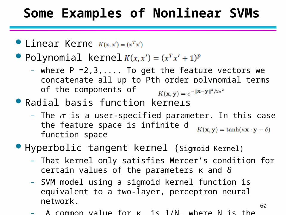
Some Examples of Nonlinear SVMs
Linear Kernel Polynomial kernels
– where P =2,3,.... To get the feature vectors we concatenate all up to Pth order polynomial terms of the components of
Radial basis function kernels– The is a user-specified parameter. In this case the feature space 𝜎
is infinite dimensional function space
Hyperbolic tangent kernel (Sigmoid Kernel)
– That kernel only satisfies Mercer’s condition for certain values of the parameters κ and δ
– SVM model using a sigmoid kernel function is equivalent to a two-layer, perceptron neural network.
– A common value for κ is 1/N, where N is the data dimension
– A nice Paper for further information.

61
Polynomial Kernel SVM Example
Slide from Tommi S.Jaakkola, MIT

62
RBF Kernel SVM Example
Kernel we are using:
Notice that: Decrease sigma, moves towards nearest neighbor classifier
Slides from A. Zisserman

63
RBF Kernel SVM Example
Kernel we are using:
Notice that:
Decrease C, gives wider (soft) margin
Slides from A. Zisserman
64
Global Solutions and Uniqueness
Fact: – Training an SVM amounts to solving a convex quadratic
programming problem.
– A proper kernel must satisfy Mercer's positivity condition.
Notes from optimization theorem. – If the objective function is strictly convex, the solution is
guaranteed to be unique.
– For quadratic programming problems, convexity of the objective function is equivalent to positive semi-definiteness of the Hessian, and strict convexity, to positive definiteness.
– For loosely convex (convex but not strictly convex), one must examine case by case, to determine uniqueness.

66
Global Solutions and Uniqueness
So, if the Hessian is positive definite, we are happy to announce that the solution for the flowing function is unique.
(Quick reminder: Hessian is square matrix of second-order partial derivatives of a function)
What if Hessian is positive semi-definite, namely the objective function is loosely convex?
– There is necessary and sufficient condition proposed by J.C.Burge etc. For further info: Paper.
– non-uniqueness of the SVM solution will be the exception rather than the rule
The object function
Hessian

67
Thanks
Pic by Mark. A. Hicks