12.2.1TransformingwithPowersandRootsWhenyouvisitapizzaparlor,youorderapizzabyitsdiameter—say,10inches,12inches,or14inches.Buttheamountyougettoeatdependsontheareaofthepizza.Theareaofacircleisπtimesthesquareofitsradiusr.SotheareaofaroundpizzawithdiameterxisThisisapowermodeloftheformy=axpwitha=π/4andp=2Althoughapowermodeloftheformy=axpdescribestherelationshipbetweenxandyineachofthesesettings,thereisalinearrelationshipbetweenxpandy.Ifwetransformthevaluesoftheexplanatoryvariablexbyraisingthemtotheppower,andgraphthepoints(xp,y),thescatterplotshouldhavealinearform.Thefollowingexampleshowswhatwemean.Example–GoFishTransformingwithPowersImaginethatyouhavebeenputinchargeoforganizingafishingtournamentinwhichprizeswillbegivenfortheheaviestAtlanticOceanrockfishcaught.Youknowthatmanyofthefishcaughtduringthetournamentwillbemeasuredandreleased.Youarealsoawarethatusingdelicatescalestotrytoweighafishthatisfloppingaroundinamovingboatwillprobablynotyieldveryaccurateresults.Itwouldbemucheasiertomeasurethelengthofthefishwhileontheboat.Whatyouneedisawaytoconvertthelengthofthefishtoitsweight.Youcontactthenearbymarineresearchlaboratory,andtheyprovidereferencedataonthelength(incentimeters)andweight(ingrams)forAtlanticOceanrockfishofseveralsizesThefigurebelow(left)isascatterplotofthedata;notetheclearcurvedshape.Becauselengthisone-dimensionalandweight(likevolume)isthree-dimensional,apowermodeloftheformweight=a(length)3shoulddescribetherelationship.Whathappensifwecubethelengthsinthedatatableandthengraphweightversuslength3?Thefigurebelow(right)givesustheanswer.Thistransformationoftheexplanatoryvariablehelpsusproduceagraphthatisquitelinear.

There’sanotherwaytotransformthedataintheaboveexampletoachievelinearity.

Wecantakethecuberootoftheweightvaluesandgraph versuslength.Thefigurebelowshowsthattheresultingscatterplothasalinearform.Whydoesthistransformationwork?Startwithweight=a(length)3andtakethecuberootofbothsidesoftheequation:

Thatis,thereisalinearrelationshipbetweenlengthand .Oncewestraightenoutthecurvedpatternintheoriginalscatterplot,wefitaleast-squareslinetothetransformeddata.Thislinearmodelcanbeusedtopredictvaluesoftheresponsevariabley.Theresidualsandther2-valuetellushowwelltheregressionlinefitsthedata.Example–GoFishHereisMinitaboutputfromseparateregressionanalysesofthetwosetsoftransformedAtlanticOceanrockfishdata.

PROBLEM:Doeachofthefollowingforbothtransformations.(a)Givetheequationoftheleast-squaresregressionline.Defineanyvariablesyouuse.

Transformation1:

Transformation2: (b)SupposeacontestantinthefishingtournamentcatchesanAtlanticOceanrockfishthat’s36centimeterslong.Usethemodelfrompart(a)topredictthefish’sweight.Showyourwork.

Transformation1: gramsTransformation2:

grams

(c)Interpretthevalueofsincontext.ForTransformation1,thestandarddeviationoftheresidualsiss=18.841grams.Predictionsoffishweightusingthismodelwillbeoffbyanaverageofabout19grams.ForTransformation2,s=0.12.Thatis,predictionsofthecuberootoffishweightusingthismodelwillbeoffbyanaverageofabout0.12.Whenexperienceortheorysuggeststhattherelationshipbetweentwovariablesisdescribedbyapowermodeloftheformy=axp,younowhavetwostrategiesfortransformingthedatatoachievelinearity.

• 1.Raisethevaluesoftheexplanatoryvariablextotheppowerandplotthepoints(xp,y).

• 2.Takethepthrootofthevaluesoftheresponsevariableyandplotthepoints .Whatifyouhavenoideawhatpowertochoose?Youcouldguessandtestuntilyoufindatransformationthatworks.Sometechnologycomeswithbuilt-inslidersthatallowyoutodynamicallyadjustthepowerandwatchthescatterplotchangeshapeasyoudo.Itturnsoutthatthereisamuchmoreefficientmethodforlinearizingacurvedpatterninascatterplot.Insteadoftransformingwithpowersandroots,weuselogarithms.Thismoregeneralmethodworkswhenthedatafollowanunknownpowermodeloranyofseveralothercommonmathematicalmodels.

12.2.2TransformingwithLogarithmsTherelationshipbetweenlifeexpectancyandincomeperpersonisdescribedbyalogarithmicmodeloftheformy=a+blogx.Wecanusethismodeltopredicthowlongacountry’scitizenswilllivefromhowmuchmoneytheymake.FortheUnitedStates,whichhasincomeperpersonof$41,256.10,predictedlifeexpectancy=11.7+15.04log(41,256.1)=81.117yearsTheactualU.S.lifeexpectancyin2009was79.43years.

Takingthelogarithmoftheincomeperpersonvaluesstraightenedoutthecurvedpatternintheoriginalscatterplot.Thelogarithmtransformationcanalsohelpachievelinearitywhentherelationshipbetweentwovariablesisdescribedbyapowermodeloranexponentialmodel.ExponentialModelsAlinearmodelhastheformy=a+bx.Thevalueofyincreases(ordecreases)ataconstantrateasxincreases.Theslopebdescribestheconstantrateofchangeofalinearmodel.Thatis,foreach1unitincreaseinx,themodelpredictsanincreaseofbunitsiny.Youcanthinkofalinearmodelasdescribingtherepeatedadditionofaconstantamount.Sometimestherelationshipbetweenyandxisbasedonrepeatedmultiplicationbyaconstantfactor.Thatis,eachtimexincreasesby1unit,thevalueofyismultipliedbyb.ExponentialmodelAnexponentialmodeloftheformy=abxdescribessuchmultiplicativegrowth.

Populationsoflivingthingstendtogrowexponentiallyifnotrestrainedbyoutsidelimitssuchaslackoffoodorspace.Morepleasantly(unlesswe’retalkingaboutcreditcarddebt!),moneyalsodisplaysexponentialgrowthwheninterestiscompoundedeachtimeperiod.Compoundingmeansthatlastperiod’sincomeearnsincomeinthenextperiod.Example–Money,Money,MoneyUnderstandingexponentialgrowthSupposethatyouinvest$100inasavingsaccountthatpays6%interestcompoundedannually.Afterayear,youwillhaveearned$100(0.06)=$6.00ininterest.Yournewaccountbalanceistheinitialdepositplustheinterestearned:$100+($100)(0.06),or$106.Wecanrewritethisas$100(1+0.06),ormoresimplyas$100(1.06).Thatis,6%annualinterestmeansthatanyamountondepositfortheentireyearismultipliedby1.06.Ifyouleavethemoneyinvestedforasecondyear,yournewbalancewillbe[$100(1.06)](1.06)=$100(1.06)2=$112.36.Noticethatyouearn$6.36ininterestduringthesecondyear.That’sanother$6ininterestfromyourinitial$100depositplustheinterestonyour$6interestearnedforYear1.Afterxyears,youraccountbalanceyisgivenbytheexponentialmodely=100(1.06)x.Theaccompanyingtableshowsthebalanceinyoursavingsaccountattheendofeachofthefirstsixyears.Thefigureshowsthegrowthinyourinvestmentover100years.Itischaracteristicofexponentialgrowththattheincreaseappearsslowforalongperiodandthenseemstoexplode.

Ifanexponentialmodeloftheformy=abxdescribestherelationshipbetweenxandy,wecanuselogarithmstotransformthedatatoproducealinearrelationship.Startbytakingthelogarithm(we’llusebase10,butthenaturallogarithmlnusingbaseewouldworkjustaswell).Thenusealgebraicpropertiesoflogarithmstosimplifytheresultingexpressions.Herearethedetails:Wecanthenrearrangethefinalequationaslogy=loga+(logb)x.Noticethatlogaandlogbareconstantsbecauseaandbareconstants.Sotheequationgivesalinearmodelrelatingtheexplanatoryvariablextothetransformedvariablelogy.Thus,iftherelationshipbetweentwovariablesfollowsanexponentialmodel,andweplotthelogarithm(base10orbasee)ofyagainstx,weshouldobserveastraight-linepatterninthetransformeddata.Ifwefitaleast-squaresregressionlinetothetransformeddata,wecanfindthepredictedvalueofthelogarithmofyforanyvalueoftheexplanatoryvariablexbysubstitutingourx-valueintotheequationoftheline.Toobtainthecorrespondingpredictionfortheresponsevariabley,wehaveto“undo”thelogarithmtransformationtoreturntotheoriginalunitsofmeasurement.Onewayofdoingthisistousethedefinitionofalogarithmasanexponent:

Forinstance,ifwehavelogy=2,then

Ifinsteadwehavelny=2,then

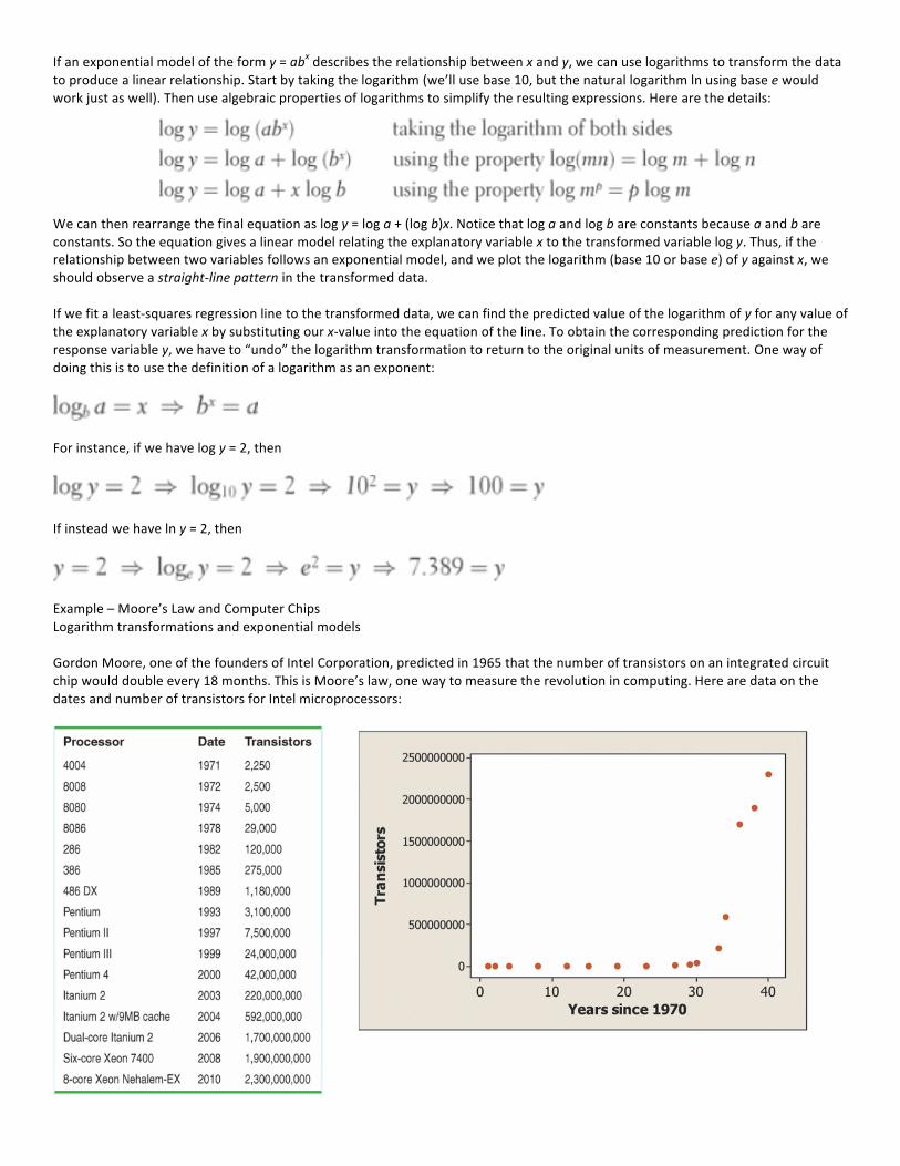
Example–Moore’sLawandComputerChipsLogarithmtransformationsandexponentialmodelsGordonMoore,oneofthefoundersofIntelCorporation,predictedin1965thatthenumberoftransistorsonanintegratedcircuitchipwoulddoubleevery18months.ThisisMoore’slaw,onewaytomeasuretherevolutionincomputing.HerearedataonthedatesandnumberoftransistorsforIntelmicroprocessors:

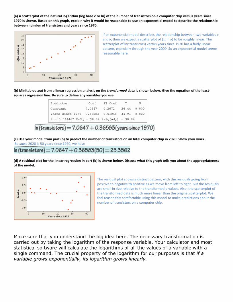
(a)Ascatterplotofthenaturallogarithm(logbaseeorln)ofthenumberoftransistorsonacomputerchipversusyearssince1970isshown.Basedonthisgraph,explainwhyitwouldbereasonabletouseanexponentialmodeltodescribetherelationshipbetweennumberoftransistorsandyearssince1970.

Ifanexponentialmodeldescribestherelationshipbetweentwovariablesxandy,thenweexpectascatterplotof(x,lny)toberoughlylinear.Thescatterplotofln(transistors)versusyearssince1970hasafairlylinearpattern,especiallythroughtheyear2000.Soanexponentialmodelseemsreasonablehere.

(b)Minitaboutputfromalinearregressionanalysisonthetransformeddataisshownbelow.Givetheequationoftheleast-squaresregressionline.Besuretodefineanyvariablesyouuse.

(c)Useyourmodelfrompart(b)topredictthenumberoftransistorsonanIntelcomputerchipin2020.Showyourwork.Because2020is50yearssince1970,wehave

(d)Aresidualplotforthelinearregressioninpart(b)isshownbelow.Discusswhatthisgraphtellsyouabouttheappropriatenessofthemodel.

Theresidualplotshowsadistinctpattern,withtheresidualsgoingfrompositivetonegativetopositiveaswemovefromlefttoright.Buttheresidualsaresmallinsizerelativetothetransformedy-values.Also,thescatterplotofthetransformeddataismuchmorelinearthantheoriginalscatterplot.Wefeelreasonablycomfortableusingthismodeltomakepredictionsaboutthenumberoftransistorsonacomputerchip.

Make sure that you understand the big idea here. The necessary transformation is carried out by taking the logarithm of the response variable. Your calculator and most statistical software will calculate the logarithms of all the values of a variable with a single command. The crucial property of the logarithm for our purposes is that if a variable grows exponentially, its logarithm grows linearly.

CHECKYOURUNDERSTANDINGThe following table gives the resident population of the United States from 1790 to 1880, in millions of people:

The graph at the left below is a scatterplot of these data using years since 1700 as the explanatory variable. A plot of the natural logarithms of the population values against years since 1700 is shown at the right below.

1. Explain why it would be reasonable to use an exponential model to describe the relationship between the U.S. population in the years 1790 to 1880 and the number of years since 1700. Here is some Minitab output from a linear regression analysis on the transformed data.

2. Give the equation of the least-squares regression line. Define any variables you use. 3. Use this linear model to predict the U.S. population in 1890. Show your work.

4. Based on the residual plot, do you expect your prediction to be too high or too low? Justify your answer.

PowerModelsAgainBiologistshavefoundthatmanycharacteristicsoflivingthingsaredescribedquitecloselybypowermodels.Therearemoremicethanelephants,andmorefliesthanmice—theabundanceofspeciesfollowsapowermodelwithbodyweightastheexplanatoryvariable.Sodopulserate,lengthoflife,thenumberofeggsabirdlays,andsoon.Sometimesthepowerscanbepredictedfromgeometry,butsometimestheyaremysterious.Why,forexample,doestherateatwhichanimalsuseenergygoupasthe3/4poweroftheirbodyweight?BiologistscallthisrelationshipKleiber’slaw.Ithasbeenfoundtoworkallthewayfrombacteriatowhales.Thesearchgoesonforsomephysicalorgeometricalexplanationforwhylifefollowspowerlaws.Whenweapplythelogarithmtransformationtotheresponsevariableyinanexponentialmodel,weproducealinearrelationship.Toachievelinearityfromapowermodel,weapplythelogarithmtransformationtobothvariables.Herearethedetails:1.Apowermodelhastheformy=axp,whereaandpareconstants.2.Takethelogarithmofbothsidesofthisequation.Usingpropertiesoflogarithms,logy=log(axp)=loga+log(xp)=loga+plogxTheequationlogy=loga+plogxshowsthattakingthelogarithmofbothvariablesresultsinalinearrelationshipbetweenlogxandlogy.3.Lookcarefully:thepowerpinthepowermodelbecomestheslopeofthestraightlinethatlinkslogytologx.Ifapowermodeldescribestherelationshipbetweentwovariables,ascatterplotofthelogarithmsofbothvariablesshouldproducealinearpattern.Thenwecanfitaleast-squaresregressionlinetothetransformeddataandusethelinearmodeltomakepredictions.

Example–What’saPlanetAnyway?PowermodelsandlogarithmtransformationsOnJuly31,2005,ateamofastronomersannouncedthattheyhaddiscoveredwhatappearedtobeanewplanetinoursolarsystem.TheyhadfirstobservedthisobjectalmosttwoyearsearlierusingatelescopeatCaltech’sPalomarObservatoryinCalifornia.OriginallynamedUB313,thepotentialplanetisbiggerthanPlutoandhasanaveragedistanceofabout9.5billionmilesfromthesun.(Forreference,Earthisabout93millionmilesfromthesun.)Couldthisnewastronomicalbody,nowcalledEris,beanewplanet?Atthetimeofthediscovery,therewerenineknownplanetsinoursolarsystem.Herearedataonthedistancefromthesunandperiodofrevolutionofthoseplanets.Notethatdistanceismeasuredinastronomicalunits(AU),thenumberofearthdistancestheobjectisfromthesun.

Thegraphsbelowshowtheresultsoftwodifferenttransformationsofthedata.Figure(a)plotsthenaturallogarithmofperiodagainstdistancefromthesunforall9planets.Figure(b)plotsthenaturallogarithmofperiodagainstthenaturallogarithmofdistancefromthesunforthe9planets.

(a)Explainwhyapowermodelwouldprovideamoreappropriatedescriptionoftherelationshipbetweenperiodofrevolutionanddistancefromthesunthananexponentialmodel.Thescatterplotofln(period)versusdistanceisclearlycurved,soanexponentialmodelwouldnotbeappropriate.However,thegraphofln(period)versusln(distance)hasastronglinearpattern,indicatingthatapowermodelwouldbemoreappropriate.(b)Minitaboutputfromalinearregressionanalysisonthetransformeddatainfigureb(above)isshownbelow.Givetheequationoftheleast-squaresregressionline.Besuretodefineanyvariablesyouuse.

(c)Useyourmodelfrompart(b)topredicttheperiodofrevolutionforEris,whichis9,500,000,000/93,000,000=102.15AUfromthesun.Showyourwork.Eris’saveragedistancefromthesunis102.15AU.Usingthisvaluefordistanceinourmodelfrompart(b)gives

Topredicttheperiod,wehavetoundothelogarithmtransformation:

Wewouldn’twanttowaitforEristomakeafullrevolutiontoseeifourpredictionisaccurate!(d)Aresidualplotforthelinearregressioninpart(b)isshownbelow.Doyouexpectyourpredictioninpart(c)tobetoohigh,toolow,orjustright?Justifyyouranswer.

(d)Eris’svalueforln(distance)is6.939,whichwouldfallatthefarrightoftheresidualplot,wherealltheresidualsarepositive.Becauseresidual=actualy−predictedyseemslikelytobepositive,wewouldexpectourpredictiontobetoolow.