126-1

The Proportional Effect of Spatial Variables

J. G. Manchuk, O. Leuangthong and C. V. Deutsch

Centre for Computational Geostatistics, Department of Civil and Environmental Engineering

University of Alberta

Most regionalized variables exhibit a proportional effect, that is, increased variability in high valued areas. Geostatistical practice has evolved to use tools such as correlograms and Gaussian techniques that mitigate the challenges presented by the proportional effect. Nevertheless, the proportional effect is becoming increasingly important with use of multiscale data, direct simulation and unstructured grids. The early concern with the proportional effect was the complicating affect on variogram calculation; the local sill of the variogram is location dependent. Now, we are also concerned about the variance and shape of conditional distributions. The procedures to understand and model a proportional effect for variogram modeling are very different from the procedures for inference of conditional distributions. A review of the proportional effect is presented in both contexts. The proportional effect is explained and recommendations are made for each case.

Introduction 

The proportional effect is mentioned in virtually every book on geostatistics. The dominant theme of geostatistics is the mapping of regionalized variables and quantification of uncertainty. These variables are not constant over the study area; there are regions of high and low values. The key observation behind the proportional effect is that high valued areas are often more variable than low valued areas. This is observed with most earth science datasets because of the positive skewness of the histograms. The relationship between the local mean and the local variance is referred to as the proportional effect. We review the historical perspective of the proportional effect and explain why there is renewed interest in the phenomenon.

Some of the earliest references to the proportional effect were the classic references of Geostatistical Ore Reserve Estimation and Mining Geostatistics:

“The proportional effect … the standard deviation of samples within a zone is directly proportional to their mean grade.” David, 1977, page 171.

“In practice of mining applications, it has been observed that experimental semi-variograms γ(h,xo), γ(h,xo’),…, defined on different neighbourhoods V(xo), V(xo’),…,can be made to coincide by dividing each one of them by a function of the corresponding experimental mean m*(xo), m*(xo’), of the data available in each neighbourhood.” Journel and Huijbregts, 1978, page 187

There was an implicit understanding that the skewness of the original grade variable was at least partially responsible for the proportional effect. A consequence of the proportional effect was relative variograms where the variogram measure is divided by the local mean. This view of the proportional effect is supported by the comprehensive review in Geostatistics: Modeling Spatial Uncertainty:

“Proportional Effect. Variability is sometimes higher in areas with high average values than in areas with low average values.” Chilès and Delfiner, 1999, page 56.

“… the variogram in (neighborhood) Vo is modeled as a function of h and Vo of the form γVo(h)=b(mVo)γ(h) where b is some function of the local mean mVo and γ(h) a global model.” Chilès and Delfiner, 1999, page 108.

126-2

The explanation of the proportional effect in An Introduction to Applied Geostatistics is consistent with earlier definitions:

“A scatterplot of the local means and the local standard deviations from our moving window calculations is a good way to check for a relationship between the two. If it exists, such a relationship is generally referred to as a proportional effect.” Isaaks and Srivastava, 1989, page 50.

The Geostatistical Glossary and Multilingual Dictionary presents a similar view, but mentions the variance of local error distributions:

“Proportional Effect: An heteroscedastic condition in which the variance of the error is proportional to some function of the local mean of the data values.” Olea, 1991, page 62.

A secondary reference to the proportional effect in An Introduction to Applied Geostatistics directly addresses the dependency of the local conditional distribution on the local mean:

“The improvement in the results [when using the proportional effect] is quite remarkable. If a proportional effect exists, it must be taken into account when assessing local uncertainty. By rescaling the variogram to a sill of one and locally correcting the relative kriging variance, one can build confidence intervals that reflect local conditions.” Isaaks and Srivastava, 1989, page 522-523.

There are many other relevant books on geostatistics and references to the proportional effect; the quotes presented above are representative. We see the proportional effect referred to in two distinct contexts: (1) a large-scale relationship between the local mean and local standard deviation, and (2) a dependency of the variance of local distributions on the local mean. The second context is relatively new. Early references were almost exclusively aimed at the relationship between the local mean and the local standard deviation and the consequent influence on the variogram.

The second context relates to the prediction of local uncertainty. The basic approach of geostatistics over the last fifteen years has been to model uncertainty in a hierarchical framework: (1) assess the uncertainty in geological domains (rock types or facies), then (2) establish uncertainty within the deemed stationary domains with Gaussian techniques. This approach is robust with respect to the proportional effect and the concern raised by Isaaks and Srivastava (1989) toward the end of their book (p. 522-523, see above). Experience has shown that the univariate Gaussian transformation within reasonable geological subdivisions largely removes the proportional effect.

Indicator techniques such as indicator kriging account for the proportional effect by discretizing the range of variability and accounting for different continuity of high and low values. Despite this flexibility of indicator techniques, there are shortcomings such as uncontrolled variations between high and low valued classes and heavy inference that have led to more widespread usage of Gaussian techniques.

The proportional effect is becoming important as geostatistical procedures involve more complex data sets and more geometrically complicated target models (unstructured grids and map elements of variable size). There is a move away from the Gaussian transformation and multivariate Gaussian distribution. In such cases, the proportional effect once again becomes important both for variogram inference and for the prediction of local uncertainty.

A reasonable reaction to the proportional effect has been to calculate moving window statistics over the study area, perhaps within rock types, and observe the relationship between the mean and standard deviation. A strong relationship would motivate the use of correlograms or relative variograms. It is problematic, however, to quantitatively fit the relationship between the local mean and standard deviation and apply the results to uncertainty prediction. This is developed below. First, we explain the relationship of the proportional effect to the variogram, the histogram and the lognormal distributions.

Proportional effect and the variogram 

As the references above indicate, the proportional effect is commonly described in the context of the variogram being different in different areas. In practice, it was observed that the variograms could be made equal by dividing by a function of the experimental mean:

126-3

( )( )( )

( )( )( )'

0

'0

0

0 ,,umfu

umfu hh γγ

≈ (1)

The two variograms ( )0,uhγ and ( )'0,uhγ are said to differ from each other by a proportional effect.

The proportional effect function f must be determined from the data. As mentioned, it is often quadratic. This leads to a stationary variogram model ( )h0γ that is independent of location u0 such that:

( ) ( )( ) ( )hh 00*

0, γγ ⋅= umfu (2)

The correlogram (Srivastava and Parker, 1989) also mitigates the proportional effect and leads to a more stable measure of spatial correlation. Rather than calculating covariance at various lags as in the variogram, the correlogram deals with autocorrelations. Correlation at lag h is related to the covariance by Equation 3.

( ) ( )0 h

Cρ

σ σ=

⋅h

h (3)

ρ(h) and C(h) are the correlation and covariance at lag h respectively and σ0 and σh are the standard deviations at the origin and at lag h away. This permits for any non-stationary features of the variance, such as a proportional effect, to be obscured by standardizing the covariance for each lag h.

The normal score transform also mitigates the proportional effect (Verly, 1983). The proportional effect is a heteroscedastic feature of data in their original units. If the distribution happens to be Gaussian, then the conditional variance is theoretically homoscedastic or unchanging. There is no relationship between the mean and variance for normally distributed data and the normal score transform takes advantage of this result. Transforming the data to be normal almost always removes any proportional effect while back transformation will re-instate that heteroscedastic feature. Of course, this only holds if the data are multivariate Gaussian after a univariate transformation. Departures from a multivariate Gaussian distribution may lead to a small remnant proportional effect even after univariate transformation.

Geostatistical calculations related to volume variance require the variogram of the original variable. Volume variance operations include calculation of the volume-dependent variance of the random variable, that is, the dispersion variance:

( ) ( ){ }22 , v VD v V E z m= − (4)

The block values are defined at block support volume v within a larger volume support V for the mean values and V represents either a large panel or the entire area of interest. This is a well established paradigm in geostatistics. The expansion of the expected value in Equation 4 and simplification in terms of average covariances or variograms is also well established. The result:

( ) ( ) ( )2 , , ,D v V V V v vγ γ= − (5)

( ),V Vγ and ( ),v vγ are average variogram values integrated over the two support volumes v and V. The variogram required for the average variogram calculation is the variogram of the Z-variable, not the normal scores transform and not the correlogram. In most cases, the dispersion variance D2(v,V) will be too high because the variogram of normal scores and the correlogram show more spatial structure (higher covariances / lower variograms) than the original Z-variable.

The direct calculation of dispersion variance (Equation 5) is supplemented with or replaced by simulation, that is, the variable is simulated at a fine scale over domain V, then the small scale values are averaged to the larger v scale (Journel and Kyriakidis, 2002). The variogram of Z is not required in the common Gaussian simulation; the need for a Z variogram is for analytical calculations or for checking.

126-4

Historically, the proportional effect was of concern because the local variations in the variogram would affect volume variance relations and local estimation. The dependence of the proportional effect on the histogram is important.

Proportional effect and the histogram 

The multivariate Gaussian distribution has no proportional effect. This result can be explained from one of the properties of multivariate normal distributions: all conditional distributions are also (multivariate) normal (Johnson and Wichern, 2002). A multivariate normal distribution is defined by a mean vector m and covariance matrix Σ.

( ),pN= ∑X m (6)

Np is a p-variate normal distribution and X is a set of p variables. The conditional q-variate normal distribution is fully defined by a conditional mean and variance. These parameters are calculated by first partitioning Equation 6 as follows.

x x 1 11 12

x x 2 21 22

, ,q q q p qq qp p

p q q p q p qp q p q

N N−

− − −− −

⎛ ⎞∑ ∑ ⎛ ⎞∑ ∑⎡ ⎤⎡ ⎤ ⎡ ⎤ ⎡ ⎤ ⎡ ⎤= =⎜ ⎟ ⎜ ⎟⎢ ⎥⎢ ⎥ ⎢ ⎥ ⎢ ⎥ ⎢ ⎥⎜ ⎟∑ ∑ ∑ ∑⎣ ⎦ ⎣ ⎦⎣ ⎦ ⎣ ⎦ ⎣ ⎦ ⎝ ⎠⎝ ⎠

X m mX m m

(7)

{ } ( )

{ }

12 1 12 22 2 2

12 11 12 22 21

q p q

q p q

E

Var

−−

−−

= = + ∑ ∑ −

= = ∑ −∑ ∑ ∑

X X x m x m

X X x (8)

Equation 8 shows no relationship between conditional mean and variance. The variance is constant (homoscedastic) regardless of the selection of x2.

In practice, therefore, the proportional effect can be due to (1) the histogram of the variable in original units prior to a Gaussian transform or (2) a lack of multivariate Gaussianity after univariate transformation. It is likely that the first explanation is of primary importance.

The relationship between distribution and the apparent proportional effect is shown for several analytical distributions. Figure 1 shows four symmetric distributions including the Gaussian, uniform, Cauchy and Double Exponential. Figure 2 shows four skewed distributions including Chi, Exponential, Lognormal and Gumbel. Moving window statistics were calculated for 100 regions each containing 20 values. Gaussian, Uniform and Double exponential show no relationship. The Cauchy distribution shows a decreasing variance with the mean towards zero and increasing variance towards +∞. The Chi, Exponential and Lognormal data show increasing variance with mean. The Gumbel (minimum) distribution, which is negatively skewed, shows a negative correlation between mean and variance.

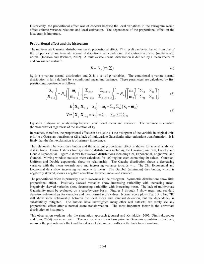
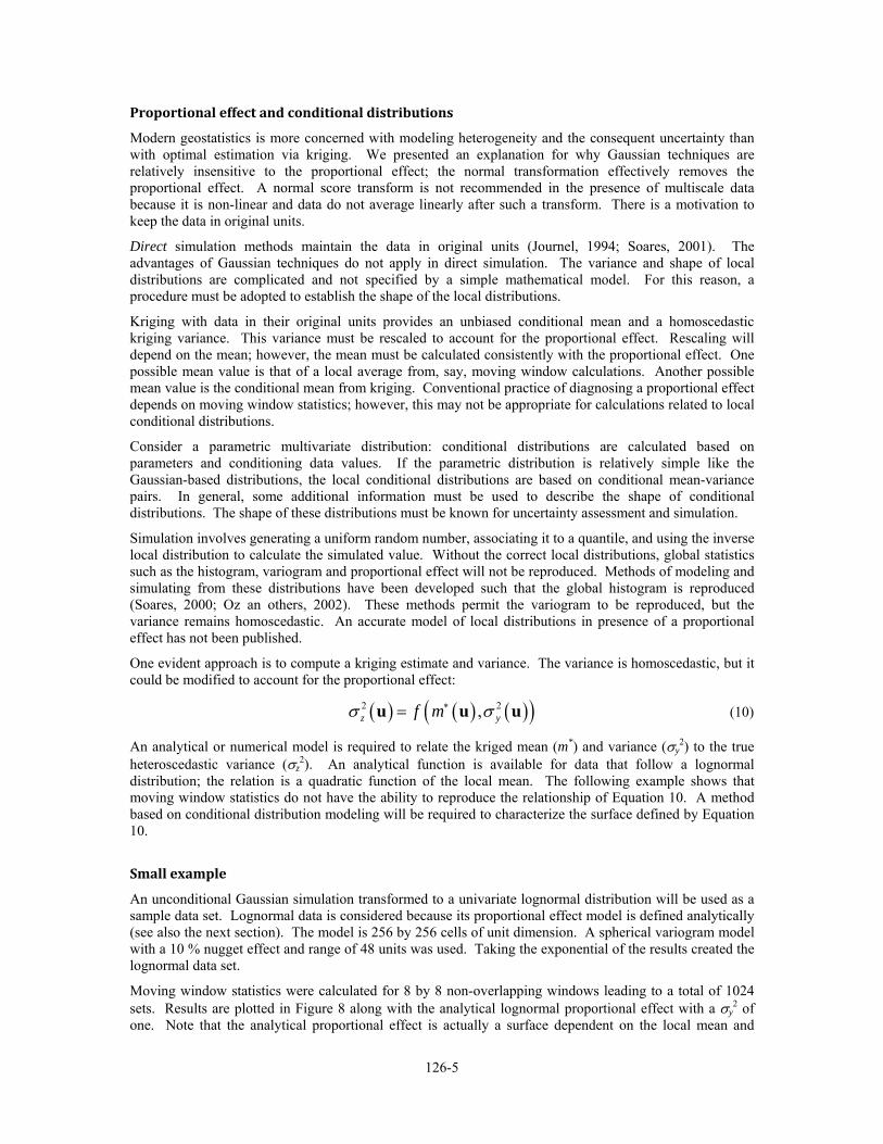
The proportional effect is primarily due to skewness in the histogram. Symmetric distributions show little proportional effect. Positively skewed variables show increasing variability with increasing mean. Negatively skewed variables show decreasing variability with increasing mean. The lack of multivariate Gaussianity must be evaluated on a case-by-case basis. Figures 3 through 7 show mean and standard deviation relationships for variables and their normal score values. Normal score plots (Fig. 3B to Fig. 7B) still show some relationship between the local mean and standard deviation, but the dependency is substantially mitigated. The authors have investigated many other real datasets; we rarely see any proportional effect after a normal score transformation. The most important factor is the univariate distribution or histogram.

This observation explains why the simulation approach (Journel and Kyriakidis, 2002; Dimitrakopoulos and Luo, 2004) works so well. The normal score transform prior to Gaussian simulation effectively removes the proportional effect and then it is included in the results via the back transformation.

126-5

Proportional effect and conditional distributions 

Modern geostatistics is more concerned with modeling heterogeneity and the consequent uncertainty than with optimal estimation via kriging. We presented an explanation for why Gaussian techniques are relatively insensitive to the proportional effect; the normal transformation effectively removes the proportional effect. A normal score transform is not recommended in the presence of multiscale data because it is non-linear and data do not average linearly after such a transform. There is a motivation to keep the data in original units.

Direct simulation methods maintain the data in original units (Journel, 1994; Soares, 2001). The advantages of Gaussian techniques do not apply in direct simulation. The variance and shape of local distributions are complicated and not specified by a simple mathematical model. For this reason, a procedure must be adopted to establish the shape of the local distributions.

Kriging with data in their original units provides an unbiased conditional mean and a homoscedastic kriging variance. This variance must be rescaled to account for the proportional effect. Rescaling will depend on the mean; however, the mean must be calculated consistently with the proportional effect. One possible mean value is that of a local average from, say, moving window calculations. Another possible mean value is the conditional mean from kriging. Conventional practice of diagnosing a proportional effect depends on moving window statistics; however, this may not be appropriate for calculations related to local conditional distributions.

Consider a parametric multivariate distribution: conditional distributions are calculated based on parameters and conditioning data values. If the parametric distribution is relatively simple like the Gaussian-based distributions, the local conditional distributions are based on conditional mean-variance pairs. In general, some additional information must be used to describe the shape of conditional distributions. The shape of these distributions must be known for uncertainty assessment and simulation.

Simulation involves generating a uniform random number, associating it to a quantile, and using the inverse local distribution to calculate the simulated value. Without the correct local distributions, global statistics such as the histogram, variogram and proportional effect will not be reproduced. Methods of modeling and simulating from these distributions have been developed such that the global histogram is reproduced (Soares, 2000; Oz an others, 2002). These methods permit the variogram to be reproduced, but the variance remains homoscedastic. An accurate model of local distributions in presence of a proportional effect has not been published.

One evident approach is to compute a kriging estimate and variance. The variance is homoscedastic, but it could be modified to account for the proportional effect:

( ) ( ) ( )( )2 2,z yf mσ σ∗=u u u (10)

An analytical or numerical model is required to relate the kriged mean (m*) and variance (σy2) to the true

heteroscedastic variance (σz2). An analytical function is available for data that follow a lognormal

distribution; the relation is a quadratic function of the local mean. The following example shows that moving window statistics do not have the ability to reproduce the relationship of Equation 10. A method based on conditional distribution modeling will be required to characterize the surface defined by Equation 10.

Small example 

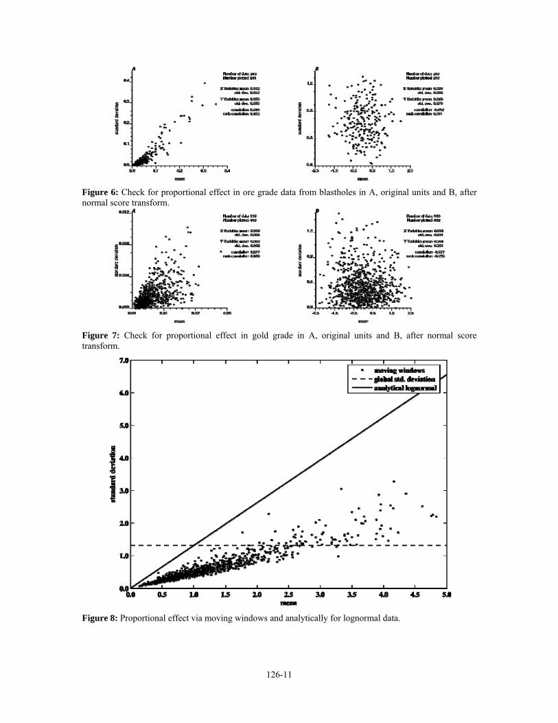
An unconditional Gaussian simulation transformed to a univariate lognormal distribution will be used as a sample data set. Lognormal data is considered because its proportional effect model is defined analytically (see also the next section). The model is 256 by 256 cells of unit dimension. A spherical variogram model with a 10 % nugget effect and range of 48 units was used. Taking the exponential of the results created the lognormal data set.

Moving window statistics were calculated for 8 by 8 non-overlapping windows leading to a total of 1024 sets. Results are plotted in Figure 8 along with the analytical lognormal proportional effect with a σy

2 of one. Note that the analytical proportional effect is actually a surface dependent on the local mean and

126-6

variance. The function for σy2 equal to one was chosen arbitrarily to show that moving window statistics

are not the proportional effect. In fact, almost every moving window point falls below the surface except near the zero-mean contour. This result can be visualized by adding a σy axis to Figure 8. The homoscedastic variance of each window is calculated from the Gaussian equivalent of the data.

Lognormal case 

The proportional effect is analytically known for the lognormal distribution (Crow and Shimizu, 1988). Gaussian data will be referred to as Y and lognormal as Z. It is shown in Figure 9 by overlaying conditional distributions from the bivariate form of both data types. For Y, the variance is homoscedastic and is independent of the mean. The conditional variance for Z is related to the mean as well as the variance of the natural logarithm of Z. Equation 11 describes the heteroscedastic relationship or proportional effect of a lognormal random variable. This is supported by Figure 9.

( )( )2 2 2exp 1Z Z ymσ σ= − (11)

This relationship is in the same form as Equation 10 above. Kriging of lognormal data in original units will provide estimates of both the conditional mean mz and the homoscedastic variance σy

2. Another interesting feature is that all conditional distributions are lognormal (Fang, Kotz, and Ng, 1990). So in the lognormal case, parameters fully define a local lognormal distribution of uncertainty from which values can be simulated. Equation 11 is used to calculate the correct variance and Equations 12 and 13 are used to characterize the distribution.

2

22ln 1 Z

Zmσβ

⎛ ⎞= +⎜ ⎟

⎝ ⎠ (12)

2

ln( )2Zm βα = − (13)

Where α and β2 are the mean and variance of ln(Z), which is normally distributed. Simulation amounts to drawing a random quantile q from a uniform distribution, inverting the standard normal distribution at q to get y and calculating the lognormal value z.

( )expz yα β= + ⋅ (14)

Extending this methodology to an arbitrary non-parametric distribution is not straightforward; however, realizing the full potential of direct methods will require such development.

Modeling the influence of a proportional effect on conditional distributions will be critical to the trend in direct methods and multiscale data in geostatistical modeling. Incorporation of multiscale information and unstructured grids is driving the need for direct simulation algorithms. To simulate data in their original units requires the shape of conditional distributions. The Gaussian and lognormal case are well understood; however, most variables do not follow any particular parametric distribution. For these, we require a proportional effect model to attain the correct conditional distribution from Kriging.

Simple models for non Gaussian distributions 

There are two evident approaches to model the proportional effect for inference of conditional distributions in original units. One is dependent on the Gaussian transform. It uses a set of non-standard normal distributions to characterize a set of conditional distributions in original units. The other method uses moving window statistics.

A relationship between the conditional mean and variance can be developed via the Gaussian transform. This relationship takes on the form of a set of conditional distributions in original units. Original-unit distributions are derived from a set of non-standard normal distributions. For a particular normal

126-7

distribution defined by a mean my and standard deviation σy, the original-unit conditional distribution can be characterized by Equation 15.

( )1 1( ) y yF G G mσ− −⎡ ⎤= ⋅ +⎣ ⎦z q (15)

Where G is the Gaussian cumulative distribution function, F is the global original-units cumulative distribution, q is a set of quantiles between 0 and 1 and z is the set of values associated with q. Together, z and q define the conditional distribution in original units. In almost all cases in geostatistical modeling, F will be a non-parametric function. F and F-1 will be evaluated numerically and z and q must be finite sets (Fig. 15).

Moving window statistics may also be used to account for a proportional effect. Consider a specific location to be estimated via kriging the surrounding data in original units: the resulting kriging variance will be homoscedastic. A window centered at the estimate location that contains the same surrounding data, or perhaps a fraction of it, can be used to calculate a local mean and variance. However, local statistics will be representative of the scale or volume of the window. Corrected to the appropriate scale, local statistics can be used to adjust conditional mean and variance values from kriging. Kriging results would then reproduce the proportional effect as interpreted from moving windows analysis.

Conclusions 

A geostatistical study involves many different considerations related to the data, decisions of stationarity, implementation choices and so on. The proportional effect is only one consideration in the big picture; however, it is important in some cases. An understanding of the historical basis for the proportional effect influences our modeling of the effect in modern applications.

The proportional effect is primarily a result of skewness in the univariate distribution. High values are more variable than low values with positively skewed distributions. The reverse is true with negatively skewed distributions. The proportional effect is observed on experimental variograms and in the variance of conditional distributions.

The proportional effect is handled when dealing with data in Gaussian units. Multigaussian kriging and Gaussian simulation with sequential or spectral methods work well. Moreover, indicator techniques also account for the proportional effect. A number of thresholds for a continuous variable are defined and used in calculation of indicator variograms and conditional distributions. The proportional effect is approximately captured by indicators in a discretized fashion. The application of geostatistical simulation to data in their original units permits the correct integration of data at different scale, but concerns of the proportional effect arise.

Geostatisticians are increasingly trying to go beyond classic Gaussian-based modeling, especially with complex data, multiscale data and the population of unstructured grids. Moving window statistics are suitable to understand the proportional effect. A quantitative model of the proportional effect is required for the inference of local distributions of uncertainty. Some approximate models are available for this purpose.

Acknowledgements 

The authors thank Canada’s NSERC organization for supporting this research. They also thank the industry sponsors of the Centre for Computational Geostatistics for partial support.

References 

Chiles, J. P., and Delfiner, P., 1999, Geostatistics: Modeling spatial uncertainty: John Wiley & Sons, 720 p.

Crow, E. L., and Shimizu, K., 1988, Lognormal distributions: Theory and applications: Marcell Dekker, 387 p.

David, M., 1977, Geostatistical ore reserve estimation: Elsevier, 364 p.

126-8

Dimitrakopoulos, R., and Luo, X., 2004, Generalized sequential Gaussian simulation: Mathematical Geology, Vol. 36, No. 3, p. 567-591.

Fang, K. T., Kotz, S., and Ng, K.W., 1990, Symmetric multivariate and related distributions: Chapman and Hall, 200 p.

Isaaks, E. H., and Srivastava, R. M., 1989, An introduction to applied geostatistics: Oxford University Press, 592 p.

Johnson, R. A., and Wichern, D. W., 2002, Applied multivariate statistical analysis: Prentice Hall, 767 p.

Journel, A. G., 1994, Modeling uncertainty: some conceptual thoughts: In Geostatistics for the Next Century (ed R. Dimitrakopoulos), Kluwer, Dordrecht, Holland, p. 30-43.

Journel, A. G., and Huijbregts, C. J., 1978, Mining geostatistics: Academic Press, 600 p.

Olea, R. A., 1991, Geostatistical glossary and multilingual dictionary: Oxford University Press, 192 p.

Oz, B., Deutsch, C. V., Tran, T. T., and Xie, Y. L., 2003, A Fortran 90 program for direct sequential simulation with histogram reproduction: Computers & Geosciences, Vol. 29, No. 1, p. 39-51.

Verly, G., 1983, The multigaussian approach and its applications to the estimation of local reserves: Mathematical Geology, Vol. 15, No. 2, p. 259-286.

Soares, A., 2001, Direct sequential simulation and cosimulation: Mathematical Geology, Vol. 33, No. 8, p. 911-926.

Srivastava, M., and Parker, H., 1989, Robust measures of spatial continuity: In Geostatistics, Proc. of the 3rd Geostatistical Congress, Armstrong ed., Kluwer publ., Holland, p. 295-308.

126-9

Figure 1: Assessments of the proportional effect using moving windows for the A, Gaussian, B, Uniform, C, Cauchy, and D, Double Exponential distributions.

Figure 2: Assessments of the proportional effect using moving windows for the A, Chi, B, Exponential, C, Lognormal, and D, Gumbel distributions.

126-10

Figure 3: Check for proportional effect with Walker Lake variables A, U in original units, B, U after normal score transform, C, V in original units, and D, V after normal score transform.

Figure 4: Check for proportional effect in transmissibility data in A, original units and B, after normal score transform.

Figure 5: Check for proportional effect in ore grade data in A, original units and B, after normal score transform.

126-11

Figure 6: Check for proportional effect in ore grade data from blastholes in A, original units and B, after normal score transform.

Figure 7: Check for proportional effect in gold grade in A, original units and B, after normal score transform.

Figure 8: Proportional effect via moving windows and analytically for lognormal data.

126-12

Figure 9: Bivariate plots of A, Gaussian distribution with correlation 0.8 and B, lognormal distribution with homoscedastic variance component 0.6.

Figure 10: Transformation process of Equation 15. Z in A is calculated starting with a probability in A that undergoes B, the non-standard normal inverse, C, the standard normal cdf and D, the inverse of the original unit global cdf.