13. generalized method of moments - lehrstuhl für...
TRANSCRIPT

13. Generalized Method of Moments
Hayashi p. 204-208
Advanced Econometrics I, Autumn 2010, Single-Equation GMM. 1

GMM Defined
The basic principle of the method of moments is to choose the parameterestimate so that the corresponding sample moments are equal to zero.
The pupulation moments in the orthogonality conditions are E[g(wi; δ)].
Its sample analogue is the sample mean of g(wi; δ) (where g(wi; δ) ≡xi · (yi − z
′iδ)) evaluated at some hypothetical value δ of δ:
gn(δ)(K×1)
≡ 1
n
n∑i=1
g(wi; δ).
Advanced Econometrics I, Autumn 2010, Single-Equation GMM. 2

GMM Defined (cont’d)
Applying the method of moments principle amounts to choosing a δ thatsolves the system of K simultaneous equations in L unknowns: gn(δ) = 0.
Because the estimation equation is linear, gn(δ) can be written as:
gn(δ) =1
n
n∑i=1
xi · (yi − z′iδ)
=1
n
n∑i=1
xi · yi −
(1
n
n∑i=1
xiz′i
)δ
≡ sxy − Sxzδ,
where sxy and Sxz are the corresponding sample moments of σxy and Σxz :
Advanced Econometrics I, Autumn 2010, Single-Equation GMM. 3

GMM Defined (cont’d)
sxy(K×1)
≡ 1
n
n∑i=1
xi · yi and Sxz(K×L)
≡ 1
n
n∑i=1
xiz′i.
So the sample analog gn(δ) = 0 is a system of K linear equations in Lunknowns:
Sxzδ = sxy.
If there are more orthogonality conditions than parameters (K > L), thenthe system may not have a solution. However, the extension of the methodof moments to cover such a case gives rise to the generalized method ofmoments (GMM).
Advanced Econometrics I, Autumn 2010, Single-Equation GMM. 4

GMM Defined (cont’d)
If the equation is exactly identified, then K = L and Σxz is square andinvertible. Ergodic stationarity means that Sxz convergs to Σxz almostsurely, Sxz is invertible for sufficiently large sample size n with probability1.
Thus, for large n; Sxzδ = sxy has a unique solution given by
δIV = S−1xz sxy =
(1
n
n∑i=1
xiz′i
)−11
n
n∑i=1
xi · yi.
This is called the iv estimator with xi serving as instruments.
Advanced Econometrics I, Autumn 2010, Single-Equation GMM. 5

GMM (cont’d)
Note:
- the formula assumes as many instruments as regressors (exactlyidentified case)
- also, if zi = xi (all the regressors being predeterminied or orthogonalto the error term), then δIV reduces to the OLS estimator.
⇒ the OLS estimator is a method of moments estimator.
⇒ the OLS estimator is a special case of the method of momentsestimator.
Advanced Econometrics I, Autumn 2010, Single-Equation GMM. 6

GMM (cont’d)
If the equation is overidentified (K > L), we cannot in general choose anL-dimensional δ to satisfy the K equations in Sxzδ = sxy.
If we cannot set gn(δ) exactly equal to 0, we can at least choose δ so thatgn(δ) is as close to 0 as possible.
This (closeness) is ensured by defining the distance between any two K-dimensional vectors ξ and η by the quadratic form
(ξ − η)′W(ξ − η),
where W, sometimes called the weighting matrix, is a symmetric andpositive definite matrix defining the distance.
Advanced Econometrics I, Autumn 2010, Single-Equation GMM. 7

GMM (cont’d)
Definition: Let W be a K × K symmetric and positive definite (p.d.)
weight matrix, possibly dependent on the sample, such that W →p W asn→∞ with W symmetric and positive definite. The GMM estimator ofδ, denoted δ(W), is
δ(W) ≡ argminδ
J(δ,W),
where
J(δ,W) ≡ n · gn(δ)′Wgn(δ).
Question: why do we multiply the distance gn(δ)′Wgn(δ) by the sample
size (n)?
Advanced Econometrics I, Autumn 2010, Single-Equation GMM. 8

GMM (cont’d)
Note:
The weighting matrix is allowed to be random and depend on the samplesize
This covers the possibility that the matrix is estimated from the sample
This definition makes clear that the GMM is a special case of minimumdistance estimation
In minimum distance estimation, plimgn(δ) = 0, as here, but the gn(·)function is not necessarily a sample mean.
Advanced Econometrics I, Autumn 2010, Single-Equation GMM. 9

GMM (cont’d)
Since gn(δ) is linear in δ, the objective function is quadratic in δ (when theequation is linear):
J(δ,W) = n · (sxy − Sxzδ)′W(sxy − Sxzδ).
The FOC for the minimization of this with respect to δ is
S′xz
(L×K)W
(K×K)sxy
(K×1)= S
′xz
(L×K)W
(K×K)Sxz
(K×L)δ
(L×1).
With the unique solution
GMM estimator : δ(W) = (S′xzWSxz)
−1S′xzWsxy.
Advanced Econometrics I, Autumn 2010, Single-Equation GMM. 10
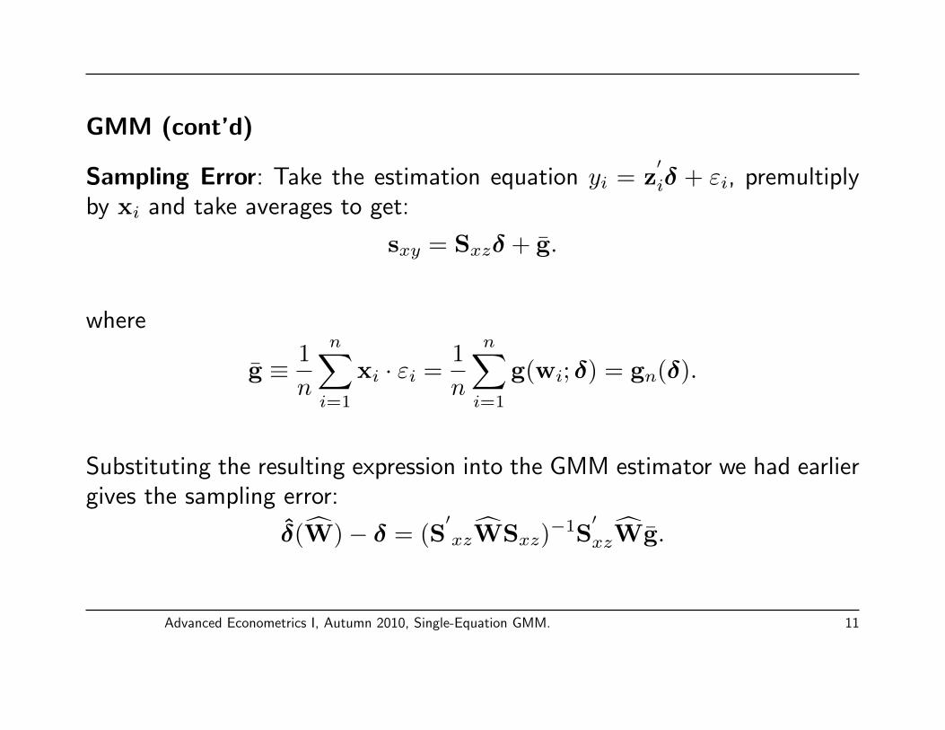
GMM (cont’d)
Sampling Error: Take the estimation equation yi = z′iδ + εi, premultiply
by xi and take averages to get:
sxy = Sxzδ + g.
where
g ≡ 1
n
n∑i=1
xi · εi =1
n
n∑i=1
g(wi; δ) = gn(δ).
Substituting the resulting expression into the GMM estimator we had earliergives the sampling error:
δ(W)− δ = (S′xzWSxz)
−1S′xzWg.
Advanced Econometrics I, Autumn 2010, Single-Equation GMM. 11

Large-Sample Properties of GMM
The GMM formula defines a set of estimators that are indexed by theweighting matrix W.
Which GMM estimators should be preferred to other GMM estimators?
Asymptotic Distribution of the GMM Estimator - The large-sampletheory for δ(W) valid for any given choice of W requires:
Proposition 3.1 (asymptotic Distribution of the GMM Estimator):
(a) (Consistency) Under linearity, ergodic stationarity, orthogonality
and rank conditions for identification, plimn→∞
δ(W) = δ
Advanced Econometrics I, Autumn 2010, Single-Equation GMM. 12

Large-Sample Properties of GMM (Cont’d)
(b) (Asymptotic Normality) With the assumption of a martingaledifference sequence,
√n((δ(W))− δ)→
dN(0,Avar(δ(W))
)as n→∞,
where
Avar(δ(W)) = (Σ′xzWΣxz)
−1Σ′xzWSWΣxz(Σ
′xzWΣxz)
−1.
Advanced Econometrics I, Autumn 2010, Single-Equation GMM. 13
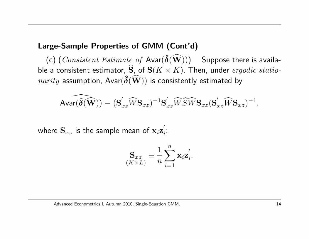
Large-Sample Properties of GMM (Cont’d)
(c) (Consistent Estimate of Avar(δ(W))) Suppose there is availa-
ble a consistent estimator, S, of S(K ×K). Then, under ergodic statio-
narity assumption, Avar(δ(W)) is consistently estimated by
Avar(δ(W)) ≡ (S
′xzWSxz)
−1S′xzW SWSxz(S
′xzWSxz)
−1,
where Sxz is the sample mean of xiz′i:
Sxz(K×L)
≡ 1
n
n∑i=1
xiz′i.
Advanced Econometrics I, Autumn 2010, Single-Equation GMM. 14

Large-Sample Properties of GMM (Cont’d)
Proving proposition 3.1 leads to three key observations:
(1) Sxz →p Σxz (by ergodic stationarity)
(2) g(≡ 1n
∑ni=1 gi)→p 0 (by ergodic stationarity and the orthogo-
nality conditions)
(3)√ng →d N(0,S) (by the assumption of a martingale difference
sequence with finite second moments)
Consistency immediately follows if we apply the 1st and 2nd proves as wellas lemma 1 (or lemma 2.3(a) as per Hayashi) on the expression for samplingerror we got earlier, i.e.,
δ(W)− δ = (S′xzWSxz)
−1S′xzWg.
Advanced Econometrics I, Autumn 2010, Single-Equation GMM. 15

Large-Sample Properties of GMM (Cont’d)
Asymptotic normality can be proved by multiplying both sides of theexpression for the Sampling Error by
√n to obtain
√n(δ(W)− δ) = (S
′xzWSxz)
−1S′xzW
√ng.
and the 3rd prove to the proposition of asymptotic distribution of the GMMestimator, lemma 1 (or lemma 2.3(a)), and lemma 5 (or lemma 2.4(c)).
Part(c) of proposition 3.1 of the GMM estimator (Consistent Estimate of
Avar(δ(W))) follows immediately from Lemma 2.3(a).
Advanced Econometrics I, Autumn 2010, Single-Equation GMM. 16

Large-Sample Properties of GMM (Cont’d)
Estimation of Error Variance:
Propostion 3.2 (consistent estimation of error variance): For any
consistent estimator, δ, of δ, define εi ≡ yi−z′iδ. Under Assumption 3.1,
3.2, plus the assumption that E(ziz′i) (second moments of the regressors)
exists and is finite,
1
n
n∑i=1
ε2i →pE(ε2i ),
provided E(ε2i ) exists and is finite.
The proof of proposition 3.2 can be shown based on the relationship betweenεi and εi
Advanced Econometrics I, Autumn 2010, Single-Equation GMM. 17

Large-Sample Properties of GMM (Cont’d)
It can be shown that
εi ≡ yi − z′iδ = εi − z
′i(δ − δ),
so that
ε2i = ε2i − 2(δ − δ)′zi · εi + (δ − δ)
′ziz
′i(δ − δ).
Summing over i, we obtain
1
n
n∑i=1
ε2i =1
n
n∑i=1
ε2i − 2(δ− δ)′ 1
n
n∑i=1
zi · εi+ (δ− δ)′(
1
n
n∑i=1
ziz′i
)(δ− δ).
Advanced Econometrics I, Autumn 2010, Single-Equation GMM. 18

Large-Sample Properties of GMM (Cont’d)
so that:
(i) 1n
∑i ε
2i →p E(ε2i ).
(ii) δ is consistent and 1n
∑i ziz
′i→p some finite matrx by assumption
⇒ the last term vanishes
(iii) E(zi · εi) exists and is finite (by the Cauchy-Schwartz inequality).By ergodic stationarity 1
n
∑i zi · εi →p some finite vector
⇒ the second term on the RHS also vanishes.
Advanced Econometrics I, Autumn 2010, Single-Equation GMM. 19

Testing Overidentifying Restrictions
If the equation is exactly identified, then it is possible to choose δ so thatall the elements of the sample moments gn(δ) are zero and the distance
J(δ,W) ≡ n · gn(δ)′Wgn(δ)
is zero. (The δ that does it is the IV estimator.)
If the equation is overidentified, then the distance cannot be set to zeroexactly, but we would expect the minimized distance to be close to zero.
If the weighting matrix W is chosen optimally so that plimW = S−1, thenthe minimized distance is asymptotically chi-squared.
Advanced Econometrics I, Autumn 2010, Single-Equation GMM. 20

Testing Overidentifying Restrictions (cont’d)
Let S a consistent estimator of S, and consider first the case where thedistance is evaluated at the true parameter value δ, J(δ,W−1).
Since by definition gn(δ) = g(≡ 1n
∑i gi) for δ = δ, the distance equals
J(δ, S−1) = n · g′S−1g = (
√ng)
′S−1(
√ng).
Since√ng →d N(0,S) and S →p S, its asymptotic distribution is χ2(K)
by lemma 6 (or lemma 2.4(d)).
Advanced Econometrics I, Autumn 2010, Single-Equation GMM. 21

Testing Overidentifying Restrictions (cont’d)
If δ is replaced by δ(S−1), then the degrees of freedom change from K toK − L.
This is because we have to estimate L parameters δ before forming thesample average gi.
Proposition 3.6 (Hansen’s test of overidentifying restrictions(Hansen,1982)): Suppose there is available a consistent estimator, S,
of S(= E(gig′i)). Under Assumption 3.1-3.5,
J(δ(S−1), S−1)(= n · gn(δ(S−1))′S−1gn(δ(S−1)))→
dχ2(K − L).
Advanced Econometrics I, Autumn 2010, Single-Equation GMM. 22

Testing Overidentifying Restrictions (cont’d): Note that:(i) the J test is a specification test, testing whether all the restrictionsof the model are satisfied
– if the J statistic of Proposition 3.6 is surprisingly large, it meansthat either the orthogonality conditions (Assumption 3.3) or the otherassumptions (or both) are likely to be false.
– only when we are certain about these assumptions can we interpretthe J statistic as evidence for the endogeneity of some of the Kinstruments included in xi.
(ii) the test is not consistent against some failures of the orthogonalityconditions. The main reason is to do with loss of degrees of freedomfrom K to K − L
(iii) the J test rejects too often in small samples (actual size of the Jtest in small samples far exceeds the nominal size).
Advanced Econometrics I, Autumn 2010, Single-Equation GMM. 23

The Efficient GMM Estimator:
For a given set of instruments xi, the GMM estimator δ(W) is defined foran arbitrary p.d. and symmetric weight matrix W.
The asymptotic variance δ(W) depends on the chosen weight matrix W.Since
avar(δ(W)) = (Σ′xzWΣxz)
−1Σ′xzWSWΣxz(Σ
′xzWΣxz)
−1.
What weight matrix W produces the smallest value of avar(δ(W))?
The GMM estimator constructed with such a weight matrix is called theefficient GMM estimator.
Advanced Econometrics I, Autumn 2010, Single-Equation GMM. 24

The Efficient GMM Estimator (cont’d):
Hansen (1982) showed that the efficient GMM estimator is arrived at bysetting W = S−1
Accordingly, W = S−1 such that
S→p
S = E[xtx′tε
2t ]
= avar(√ngn(δ0))
For this choice of W, the asymptotic variance
avar(δ(W)) = (Σ′xzWΣxz)
−1Σ′xzWSWΣxz(Σ
′xzWΣxz)
−1.
reduces to
Advanced Econometrics I, Autumn 2010, Single-Equation GMM. 25

The Efficient GMM Estimator (cont’d):
avar(δ(S−1)) = (Σ′xzS−1Σxz)
−1
of which a consistent estimate is
avar(δ(S−1)) = (S′xzS−1Sxz)
−1
The efficient GMM estimator is then defined as
δ(S−1) = argminδ
ngn(δ)′S−1gn(δ),
which requires a consistent estimate of S = E[gtg′t] = E[xtx
′tε
2t ].
Advanced Econometrics I, Autumn 2010, Single-Equation GMM. 26

The Efficient GMM Estimator (cont’d):
However, a consistent estimation of S, in turn, requires a consistent estimateof δ0.
White (1982) showed that a consistent estimate of S has the form
S =1
n
n∑t=1
xtx′tε
2t =
1
n
n∑t=1
xtx′t
(yt − z
′tδ)2.
such that δ →pδ0
Advanced Econometrics I, Autumn 2010, Single-Equation GMM. 27