generalized method of moments (gmm)
TRANSCRIPT

Chapter 6
Generalized Method Of Moments(GMM)
Note: The primary reference text for these notes is Hall (2005). Alternative, but less comprehensive,treatments can be found in chapter 14 of Hamilton (1994) or some sections of chapter 4 of Greene(2007). For an excellent perspective of GMM from a finance point of view, see chapters 10, 11 and13 in Cochrane (2001).
Generalized Moethod of Moments is a broadly applicable parameter estimation strategy whichnests the classic method of moments, linear regression, maximum likelihood. This chapterdiscusses the specification of moment conditions – the building blocks of GMM estimations,estimation, inference and specificatrion testing. These ideas are illustrated through three ex-amples: estimation of a consumption asset pricing model, linear factors models and stochasticvolatility.
Generalized Method of Moments (GMM) is an estimation procedure that allows economicmodels to be specified while avoiding often unwanted or unnecessary assumptions, such asspecifying a particular distribution for the errors. This lack of structure means GMM is widelyapplicable, although this generality comes at the cost of a number of issues, the most important ofwhich is questionable small sample performance. This chapter introduces the GMM estimationstrategy, discuss specification, estimation, inference and testing.
6.1 Classical Method of Moments
The classical method of moments, or simply method of moments, uses sample moments toestimate unknown parameters. For example, suppose a set of T observations, y1, . . . , yT are
387

i.i.d. Poisson with intensity parameter λ. Since E[yt ] = λ, a natural method to estimate theunknown parameter is to use the sample average,
λ = T −1T∑
t=1
yt (6.1)
which converges to λ as the sample size grows large. In the case of Poisson data , the mean is notthe only moment which depends on λ, and so it is possible to use other moments to learn aboutthe intensity. For example the variance V[yt ] = λ, also depends on λ and so E[y 2
t ] = λ2 + λ. This
can be used estimate to lambda since
λ + λ2 = E
[T −1
T∑t=1
y 2t
](6.2)
and, using the quadratic formula, an estimate of λ can be constructed as
λ =−1 +
√1 + 4y 2
2(6.3)
where y 2 = T −1∑T
t=1 y 2t . Other estimators for λ could similarly be constructed by computing
higher order moments of yt .1 These estimators are method of moments estimators since they usesample moments to estimate the parameter of interest. Generalized Method of Moments (GMM)extends the classical setup in two important ways. The first is to formally treat the problem ofhaving two or more moment conditions which have information about unknown parameters.GMM allows estimation and inference in systems of Q equations with P unknowns, P ≤ Q .The second important generalization of GMM is that quantities other than sample momentscan be used to estimate the parameters. GMM exploits laws of large numbers and central limittheorems to establish regularity conditions for many different “moment conditions” that may ormay not actually be moments. These two changes produce a class of estimators that is broadlyapplicable. Section 6.7 shows that the classical method of moments, ordinary least squares andmaximum likelihood are all special cases of GMM.
6.2 Examples
Three examples will be used throughout this chapter. The first is a simple consumption assetpricing model. The second is the estimation of linear asset pricing models and the final is theestimation of a stochastic volatility model.
1The quadratic formula has two solutions. It is simple to verify that the other solution,−1−
√1+4y 2
2 , is negative andso cannot be the intensity of a Poisson process.

6.2.1 Consumption Asset Pricing
GMM was originally designed as a solution to a classic problem in asset pricing: how can aconsumption based model be estimated without making strong assumptions on the distributionof returns? This example is based on L. P. Hansen and Singleton (1982), a model which builds onR. E. Lucas (1978).
The classic consumption based asset pricing model assumes that a representative agentmaximizes the conditional expectation of their lifetime discounted utility,
Et
[ ∞∑i=0
β i U (ct+i )
](6.4)
whereβ is the discount rate (rate of time preference) and U (·) is a strictly concave utility function.Agents allocate assets between N risky assets and face the budget constraint
ct +N∑
j=1
pj ,t q j ,t =N∑
j=1
R j ,t q j ,t−m j + wt (6.5)
where ct is consumption, pj ,t and q j ,t are price and quantity of asset j , j = 1, 2, . . . , N , R j ,t is thetime t payoff of holding asset j purchased in period t −m j , q j ,t−m j is the amount purchased inperiod t −m j and wt is real labor income. The budget constraint requires that consumptionplus asset purchases (LHS) is equal to portfolio wealth plus labor income. Solving this modelproduces a standard Euler equation,
pj ,t U ′(ct ) = βm j Et
[R j ,t+m j U
′(ct+m j )]
(6.6)
which is true for all assets and all time periods. This Euler equation states that the utility foregoneby purchasing an asset at pj ,t must equal the discounted expected utility gained from holdingthat asset in period t +m j . The key insight of L. P. Hansen and Singleton (1982) is that this simplecondition has many testable implications, mainly that
Et
[βm j
(R j ,t+m j
pj ,t
)(U ′(ct+m j )
U ′(ct )
)]− 1 = 0 (6.7)
Note thatR j ,t+m j
pj ,tis the gross rate of return for asset j (1 plus the net rate of return). Since the
Euler equation holds for all time horizons, it is simplest to reduce it to a one-period problem.Defining r j ,t+1 to be the net rate of return one period ahead for asset j ,
Et
[β(
1 + r j ,t+1
)(U ′(ct+1)U ′(ct )
)]− 1 = 0 (6.8)
which provides a simple testable implication of this model. This condition must be true for anyasset j which provides a large number of testable implications by replacing the returns of oneseries with those of another. Moreover, the initial expectation is conditional which produces

further implications for the model. Not only is the Euler equation required to have mean zero, itmust be uncorrelated with any time t instrument zt , and so it must also be the case that
E
[(β(
1 + r j ,t+1
)(U ′(ct+1)U ′(ct )
)− 1
)zt
]= 0. (6.9)
The use of conditioning information can be used to construct a huge number of testable restric-tions. This model is completed by specifying the utility function to be CRRA,
U (ct ) =c 1−γ
t
1− γ(6.10)
U ′(ct ) = c−γt (6.11)
where γ is the coefficient of relative risk aversion. With this substitution, the testable implicationsare
E
[(β(
1 + r j ,t+1
)( ct+1
ct
)−γ− 1
)zt
]= 0 (6.12)
where zt is any t available instrument (including a constant, which will produce an unconditionalrestriction).
6.2.2 Linear Factor Models
Linear factor models are widely popular in finance due to their ease of estimation using theE F Fama and MacBeth (1973) methodology and the Shanken (1992) correction. However, Fama-MacBeth, even with the correction, has a number of problems; the most important is that theassumptions underlying the Shanken correction are not valid for heteroskedastic asset pricingmodels and so the modified standard errors are not consistent. GMM provides a simple methodto estimate linear asset pricing models and to make correct inference under weaker conditionsthan those needed to derive the Shanken correction. Consider the estimation of the parametersof the CAPM using two assets. This model contains three parameters: the two βs, measuring therisk sensitivity, and λm , the market price of risk. These two parameters are estimated using fourequations,
r e1t = β1r e
m t + ε1t (6.13)
r e2t = β2r e
m t + ε2t
r e1t = β1λ
m + η1t
r e2t = β2λ
m + η2t
where r ej ,t is the excess return to asset j , r e
m ,t is the excess return to the market and ε j ,t and η j ,t
are errors.
These equations should look familiar; they are the Fama-Macbeth equations. The first two –the “time-series” regressions – are initially estimated using OLS to find the values for β j , j = 1, 2and the last two – the “cross-section” regression – are estimated conditioning on the first stage βsto estimate the price of risk. The Fama-MacBeth estimation procedure can be used to generate aset of equations that should have expectation zero at the correct parameters. The first two comefrom the initial regressions (see chapter 3),
(r e1t + β1r e
m t )re
m t = 0 (6.14)
(r e2t + β2r e
m t )re
m t = 0
and the last two come from the second stage regressions
r e1t − β1λ
m = 0 (6.15)
r e2t − β2λ
m = 0
This set of equations consists 3 unknowns and four equations and so cannot be directly estimatesusing least squares. One of the main advantages of GMM is that it allows estimation in systemswhere the number of unknowns is smaller than the number of moment conditions, and to testwhether the moment conditions hold (all conditions not significantly different from 0).
6.2.3 Stochastic Volatility Models
Stochastic volatility is an alternative framework to ARCH for modeling conditional heteroskedas-ticity. The primary difference between the two is the inclusion of 2 (or more) shocks in stochasticvolatility models. The inclusion of the additional shock makes standard likelihood-based meth-ods, like those used to estimate ARCH-family models, infeasible. GMM was one of the firstmethods used to estimate these models. GMM estimators employ a set of population momentconditions to determine the unknown parameters of the models. The simplest stochastic volatil-ity model is known as the log-normal SV model,
rt = σt εt (6.16)
lnσ2t = ω + ρ ln
(σ2
t−1 −ω)+ σηηt (6.17)
where (εt ,ηt )i.i.d.∼ N (0, I2) are i.i.d. standard normal. The first equation specifies the distribution
of returns as heteroskedastic normal. The second equation specifies the dynamics of the logof volatility as an AR(1). The parameter vector is (ω,ρ,ση)′. The application of GMM will usefunctions of rt to identify the parameters of the model. Because this model is so simple, it isstraight forward to derive the following relationships:
E[|rt |]=
√2
πE [σt ] (6.18)
E[
r 2t
]= E
[σ2
t
]E[|r 3
t |]= 2
√2
πE[σ3
t
]E[|r 4
t |]= 3E
[σ4
t
]E[|rt rt− j |
]=
2
πE[σtσt− j
]E[|r 2
t r 2t− j |
]= E
[σ2
tσ2t− j
]where
E[σm
t
]= exp
mω
2+m 2
σ2η
1−ρ2
8
(6.19)
E[σm
t σnt− j
]= E
[σm
t
]E[σn
t
]exp
(mn )ρ j
σ2η
1−ρ2
4
.
These conditions provide a large set of moments to determine the three unknown parameters.GMM seamlessly allows 3 or more moment conditions to be used in the estimation of theunknowns.
6.3 General Specification
The three examples show how a model – economic or statistical – can be turned into a setof moment conditional that have zero expectation, at least if the model is correctly specified.All GMM specifications are constructed this way. Derivation of GMM begins by defining thepopulation moment condition.
Definition 6.1 (Population Moment Condition). Let wt be a vector of random variables, θ 0 be ap by 1 vector of parameters, and g(·) be a q by 1 vector valued function. The population momentcondition is defined
E[g(wt , θ 0)] = 0 (6.20)
It is possible that g(·) could change over time and so could be replaced with gt (·). For clarity ofexposition the more general case will not be considered.
Definition 6.2 (Sample Moment Condition). The sample moment condition is derived from the
average population moment condition,
gT (w, θ ) = T −1T∑
t=1
g(wt , θ ). (6.21)
The gT notation dates back to the original paper of L. P. Hansen (1982) and is widely used todifferentiate population and sample moment conditions. Also note that the sample momentcondition suppresses the t in w. The GMM estimator is defined as the value of θ that minimizes
QT (θ ) = gT (w, θ )′WT gT (w, θ ). (6.22)
Thus the GMM estimator is defined as
θ = arg minθ
QT (θ ) (6.23)
where WT is a q by q positive semi-definite matrix. WT may (and generally will) depend on thedata but it is required to converge in probability to a positive definite matrix for the estimator tobe well defined. In order to operationalize the GMM estimator, q , the number of moments, willbe required to greater than or equal to p , the number of unknown parameters.
6.3.1 Identification and Overidentification
GMM specifications fall in to three categories: underidentified, just-identified and overidentified.Underidentified models are those where the number of non-redundant moment conditions is lessthan the number of parameters. The consequence of this is obvious: the problem will have manysolutions. Just-identified specification have q = p while overidentified GMM specifications haveq > p . The role of just- and overidentification will be reexamined in the context of estimation andinference. In most applications of GMM it is sufficient to count the number of moment equationsand the number of parameters when determining whether the model is just- or overidentified.The exception to this rule arises if some moment conditions are linear combination of othermoment conditions – in other words are redundant – which is similar to including a perfectlyco-linear variable in a regression.
6.3.1.1 Example: Consumption Asset Pricing Model
In the consumption asset pricing model, the population moment condition is given by
g(wt , θ 0) =
(β0 (1 + rt+1)
(ct+1
ct
)−γ0
− 1
)⊗ zt (6.24)
where θ 0 = (β0, γ0)′, and wt = (ct+1, ct , r′t+1, z′t )′ and⊗ denotes Kronecker product.2Note that
both rt+1 and zt are column vectors and so if there are n assets and k instruments, then thedimension of g(·)(number of moment conditions) is q = nk by 1 and the number of parametersis p = 2. Systems with nk ≥ 2 will be identified as long as some technical conditions are metregarding instrument validity (see section 6.11).
6.3.1.2 Example: Linear Factor Models
In the linear factor models, the population moment conditions are given by
g(wt , θ 0) =((rt − β ft )⊗ ft
rt − βλ
)(6.27)
where θ 0 = (vec(β )′,λ′)′ and wt = (r′t , f′t )′ where rt is n by 1 and ft is k by 1.3 These moments
can be decomposed into two blocks. The top block contains the moment conditions necessaryto estimate the βs. This block can be further decomposed into n blocks of k moment conditions,one for each factor. The first of these n blocks is
(r1t − β11 f1t − β12 f2t − . . .− β1K fK t ) f1t
(r1t − β11 f1t − β12 f2t − . . .− β1K fK t ) f2t
...(r1t − β11 f1t − β12 f2t − . . .− β1K fK t ) fK t
=ε1t f1t
ε1t f2t
...ε1t fK t
. (6.29)
2
Definition 6.3 (Kronecker Product). Let A = [ai j ] be an m by n matrix, and let B = [bi j ] be a k by l matrix. TheKronecker product is defined
A⊗ B =
a11B a12B . . . a1n Ba21B a22B . . . a2n B
......
......
am1B am2B . . . amn B
(6.25)
and has dimension mk by nl . If a and b are column vectors with length m and k respectively, then
a⊗ b =
a1ba2b
...am b
. (6.26)
3The vec operator stacks the columns of a matrix into a column vector.
Definition 6.4 (vec). Let A = [ai j ] be an m by n matrix. The the vec operator (also known as the stack operator) isdefined
vecA =
A1
A2
...An
(6.28)
and vec(A) is mn by 1.

Each equation in (6.29) should be recognized as the first order condition for estimating the slopecoefficients in a linear regression. The second block has the form
r1t − β11λ1 − β12λ2 − . . .− β1K λK
r2t − β21λ1 − β22λ2 − . . .− β2K λK
...rN t − βN 1λ1 − βN 2λ2 − . . .− βN K λK
(6.30)
where λ j is the risk premium on the jthfactor. These moment conditions are derived from therelationship that the average return on an asset should be the sum of its risk exposure times thepremium for that exposure.
The number of moment conditions (and the length of g(·)) is q = nk + n . The number ofparameters is p = nk (fromβ ) + k (from λ), and so the number of overidentifying restrictions isthe number of equations in g(·)minus the number of parameters, (nk + n )− (nk + k ) = n − k ,the same number of restrictions used when testing asset pricing models in a two-stage Fama-MacBeth regressions.
6.3.1.3 Example: Stochastic Volatility Model
Many moment conditions are available to use in the stochastic volatility model. It is clear thatat least 3 conditions are necessary to identify the 3 parameters and that the upper bound onthe number of moment conditions is larger than the amount of data available. For clarity ofexposition, only 5 and 8 moment conditions will be used, where the 8 are a superset of the 5.These 5 are:
g(wt , θ 0) =
|rt | −√
2π exp
(ω2 +
σ2η
1−ρ2
8
)
r 2t − exp
(ω +
σ2η
1−ρ2
2
)r 4
t − 3 exp(
2ω + 2σ2η
1−ρ2
)|rt rt−1| − 2
π
(exp
(ω2 +
σ2η
1−ρ2
8
))2
exp
(ρ
σ2η
1−ρ2
4
)
r 2t r 2
t−2 −
(exp
(ω +
σ2η
1−ρ2
2
))2
exp(ρ2 σ2
η
1−ρ2
)
(6.31)
These moment conditions can be easily verified from 6.18 and 6.19. The 8 moment-conditionestimation extends the 5 moment-condition estimation with
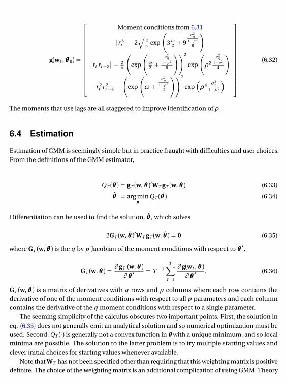
g(wt , θ 0) =
Moment conditions from 6.31
|r 3t | − 2
√2π exp
(3ω2 + 9
σ2η
1−ρ2
8
)
|rt rt−3| − 2π
(exp
(ω2 +
σ2η
1−ρ2
8
))2
exp
(ρ3
σ2η
1−ρ2
4
)
r 2t r 2
t−4 −
(exp
(ω +
σ2η
1−ρ2
2
))2
exp(ρ4 σ2
η
1−ρ2
)
(6.32)
The moments that use lags are all staggered to improve identification of ρ.
6.4 Estimation
Estimation of GMM is seemingly simple but in practice fraught with difficulties and user choices.From the definitions of the GMM estimator,
QT (θ ) = gT (w, θ )′WT gT (w, θ ) (6.33)
θ = arg minθ
QT (θ ) (6.34)
Differentiation can be used to find the solution, θ , which solves
2GT (w, θ )′WT gT (w, θ ) = 0 (6.35)
where GT (w, θ ) is the q by p Jacobian of the moment conditions with respect to θ ′,
GT (w, θ ) =∂ gT (w, θ )∂ θ ′
= T −1T∑
t=1
∂ g(wt , θ )∂ θ ′
. (6.36)
GT (w, θ ) is a matrix of derivatives with q rows and p columns where each row contains thederivative of one of the moment conditions with respect to all p parameters and each columncontains the derivative of the q moment conditions with respect to a single parameter.
The seeming simplicity of the calculus obscures two important points. First, the solution ineq. (6.35) does not generally emit an analytical solution and so numerical optimization must beused. Second, QT (·) is generally not a convex function in θwith a unique minimum, and so localminima are possible. The solution to the latter problem is to try multiple starting values andclever initial choices for starting values whenever available.
Note that WT has not been specified other than requiring that this weighting matrix is positivedefinite. The choice of the weighting matrix is an additional complication of using GMM. Theory
dictates that the best choice of the weighting matrix must satisfyWTp→ S−1 where
S = avar{√
T gT (wt , θ 0)}
(6.37)
and where avar indicates asymptotic variance. That is, the best choice of weighting is the inverseof the covariance of the moment conditions. Unfortunately the covariance of the momentconditions generally depends on the unknown parameter vector, θ 0. The usual solution is touse multi-step estimation. In the first step, a simple choice for WT ,which does not depend onθ (often Iq the identity matrix), is used to estimate θ . The second uses the first-step estimate ofθ to estimate S. A more formal discussion of the estimation of S will come later. For now, assumethat a consistent estimation method is being used so that S
p→ S and so WT = S−1 p→ S−1.
The three main methods used to implement GMM are the classic 2-step estimation, K -stepestimation where the estimation only ends after some convergence criteria is met and continuousupdating estimation.
6.4.1 2-step Estimator
Two-step estimation is the standard procedure for estimating parameters using GMM. First-stepestimates are constructed using a preliminary weighting matrix W, often the identity matrix, andθ 1 solves the initial optimization problem
2GT (w, θ 1)′WgT (w, θ 1) = 0. (6.38)
The second step uses an estimated S based on the first-step estimates θ 1. For example, if themoments are a martingale difference sequence with finite covariance,
S(w, θ 1) = T −1T∑
t=1
g(wt , θ 1)g(wt , θ 1)′ (6.39)
is a consistent estimator of the asymptotic variance of gT (·), and the second-step estimates, θ 2,minimizes
QT (θ ) = gT (w, θ )′S−1(θ 1)gT (w, θ ). (6.40)
which has first order condition
2GT (w, θ 2)′S−1(θ 1)gT (w, θ 2) = 0. (6.41)
Two-step estimation relies on the the consistence of the first-step estimates, θ 1p→ θ 0 which is
generally needed for Sp→ S.

6.4.2 k -step Estimator
The k -step estimation strategy extends the two-step estimator in an obvious way: if two-stepsare better than one, k may be better than two. The k -step procedure picks up where the 2-stepprocedure left off and continues iterating between θ and S using the most recent values θavailable when computing the covariance of the moment conditions. The procedure terminateswhen some stopping criteria is satisfied. For example if
max |θ k − θ k−1| < ε (6.42)
for some small value ε, the iterations would stop and θ = θ k . The stopping criteria shoulddepend on the values of θ . For example, if these values are close to 1, then 1× 10⁻⁴ may be agood choice for a stopping criteria. If the values are larger or smaller, the stopping criteria shouldbe adjusted accordingly. The k -step and the 2-step estimator are asymptotically equivalent,although, the k -step procedure is thought to have better small sample properties than the 2-stepestimator, particularly when it converges.
6.4.3 Continuously Updating Estimator (CUE)
The final, and most complicated, type of estimation, is the continuously updating estimator.Instead of iterating between estimation of θ and S, this estimator parametrizes S as a functionof θ . In the problem, θ C is found as the minimum of
Q CT (θ ) = gT (w, θ )′S(w, θ )−1gT (w, θ ) (6.43)
The first order condition of this problem is not the same as in the original problem since θappears in three terms. However, the estimates are still first-order asymptotically equivalent tothe two-step estimate (and hence the k -step as well), and if the continuously updating estimatorconverges, it is generally regarded to have the best small sample properties among these meth-ods.4 There are two caveats to using the continuously updating estimator. First, it is necessaryto ensure that gT (w, θ ) is close to zero and that minimum is not being determined by a largecovariance since a large S(w, θ ) will make Q C
T (θ ) small for any value of the sample momentconditions gT (w, θ ). The second warning when using the continuously updating estimator hasto make sure that S(w, θ ) is not singular. If the weighting matrix is singular, there are values ofθ which satisfy the first order condition which are not consistent. The continuously updatingestimator is usually implemented using the k -step estimator to find starting values. Once thek -step has converged, switch to the continuously updating estimator until it also converges.
4The continuously updating estimator is more efficient in the second-order sense than the 2- of k -step estimators,which improves finite sample properties.

6.4.4 Improving the first step (when it matters)
There are two important caveats to the first-step choice of weighting matrix. The first is simple:if the problem is just identified, then the choice of weighting matrix does not matter and onlyone step is needed. The understand this, consider the first-order condition which definesθ ,
2GT (w, θ )′WT gT (w, θ ) = 0. (6.44)
If the number of moment conditions is the same as the number of parameters, the solution musthave
gT (w, θ ) = 0. (6.45)
as long as WT is positive definite and GT (w, θ ) has full rank (a necessary condition). However, ifthis is true, then
2GT (w, θ )′WT gT (w, θ ) = 0 (6.46)
for any other positive definite WT whether it is the identity matrix, the asymptotic variance ofthe moment conditions, or something else.
The other important concern when choosing the initial weighting matrix is to not overweighthigh-variance moments and underweight low variance ones. Reasonable first-step estimatesimprove the estimation of S which in turn provide more accurate second-step estimates. Thesecond (and later) steps automatically correct for the amount of variability in the momentconditions. One fairly robust starting value is to use a diagonal matrix with the inverse of thevariances of the moment conditions on the diagonal. This requires knowledge about θ toimplement and an initial estimate or a good guess can be used. Asymptotically it makes nodifference, although careful weighing in first-step estimation improves the performance of the2-step estimator.
6.4.5 Example: Consumption Asset Pricing Model
The consumption asset pricing model example will be used to illustrate estimation. The dataset consists of two return series, the value-weighted market portfolio and the equally-weightedmarket portfolio, V W M and E W M respectively. Models were fit to each return series separately.Real consumption data was available from Q1 1947 until Q4 2009 and downloaded from FRED(PCECC96). Five instruments (zt ) will be used, a constant (1), contemporaneous and laggedconsumption growth (ct /ct−1 and ct−1/ct−2) and contemporaneous and lagged gross returnson the VWM (pt /pt−1 and pt−1/pt−2). Using these five instruments, the model is overidentifiedsince there are only 2 unknowns and five moment conditions,

g(wt , θ 0) =
(β (1 + rt+1)
(ct+1ct
)−γ− 1
)(β (1 + rt+1)
(ct+1ct
)−γ− 1
)ct
ct−1(β (1 + rt+1)
(ct+1ct
)−γ− 1
)ct−1
ct−2(β (1 + rt+1)
(ct+1ct
)−γ− 1
)pt
pt−1(β (1 + rt+1)
(ct+1ct
)−γ− 1
)pt−1
pt−2
(6.47)
where rt+1 is the return on either the VWM or the EWM. Table 6.1 contains parameter estimatesusing the 4 methods outlined above for each asset.
VWM EWMMethod β γ β γ
Initial weighting matrix : I5
1-Step 0.977 0.352 0.953 2.1992-Step 0.975 0.499 0.965 1.025k -Step 0.975 0.497 0.966 0.939Continuous 0.976 0.502 0.966 0.936
Initial weighting matrix: (z′z)−1
1-Step 0.975 0.587 0.955 1.9782-Step 0.975 0.496 0.966 1.004k -Step 0.975 0.497 0.966 0.939Continuous 0.976 0.502 0.966 0.936
Table 6.1: Parameter estimates from the consumption asset pricing model using both the VWMand the EWM to construct the moment conditions. The top block corresponds to using anidentity matrix for starting values while the bottom block of four correspond to using (z′z)−1 inthe first step. The first-step estimates seem to be better behaved and closer to the 2- and K -stepestimates when (z′z)−1 is used in the first step. The K -step and continuously updating estimatorsboth converged and so produce the same estimates irrespective of the 1-step weighting matrix.
The parameters estimates were broadly similar across the different estimators. The typicaldiscount rate is very low (β close to 1) and the risk aversion parameter appears to be between0.5 and 2.
One aspect of the estimation of this model is that γ is not well identified. Figure 6.1 containsurface and contour plots of the objective function as a function of β and γ for both the two-stepestimator and the CUE. It is obvious in both pictures that the objective function is steep alongthe β -axis but very flat along the γ-axis. This means that γ is not well identified and many valueswill result in nearly the same objective function value. These results demonstrate how difficult

Contours of Q in the Consumption Model2-step Estimator
γ
β
−2 0 2 4
0.9
0.95
1
1.05
−20
24
0.90.95
11.05
1
2
3
x 106
γβ
Q
Continuously Updating Estimator
γ
β
−2 0 2 4
0.9
0.95
1
1.05
−20
24
0.90.95
11.05
1
2
3x 10
6
γβ
Q
Figure 6.1: This figure contains a plot of the GMM objective function using the 2-step estimator(top panels) and the CUE (bottom panels). The objective is very steep along the β axis but nearlyflat along the γ axis. This indicates that γ is not well identified.
GMM can be in even a simple 2-parameter model. Significant care should always be taken toensure that the objective function has been globally minimized.
6.4.6 Example: Stochastic Volatility Model
The stochastic volatility model was fit using both 5 and 8 moment conditions to the returnson the FTSE 100 from January 1, 2000 until December 31, 2009, a total of 2,525 trading days.The results of the estimation are in table 6.2. The parameters differ substantially between thetwo methods. The 5-moment estimates indicate relatively low persistence of volatility withsubstantial variability. The 8-moment estimates all indicate that volatility is extremely persistentwith ρclose to 1. All estimates weighting matrix computed using a Newey-West covariance with16 lags (≈ 1.2T
13 ). A non-trivial covariance matrix is needed in this problem as the moment

conditions should be persistent in the presence of stochastic volatility, unlike in the consumptionasset pricing model which should, if correctly specified, have martingale errors.
In all cases the initial weighting matrix was specified to be an identity matrix, althoughin estimation problems such as this where the moment condition can be decomposed intog(wt , θ ) = f(wt )− h(θ ) a simple expression for the covariance can be derived by noting that, ifthe model is well specified, E[g(wt , θ )] = 0 and thus h(θ ) = E[f(wt )]. Using this relationship thecovariance of f(wt ) can be computed replacing h(θ )with the sample mean of f(wt ).
Method ω ρ ση5 moment conditions
1-Step 0.004 1.000 0.0052-Step -0.046 0.865 0.491k -Step -0.046 0.865 0.491Continuous -0.046 0.865 0.491
8 moment conditions
1-Step 0.060 1.000 0.0052-Step -0.061 1.000 0.005k -Step -0.061 1.000 0.004Continuous -0.061 1.000 0.004
Table 6.2: Parameter estimates from the stochastic volatility model using both the 5- and 8-moment condition specifications on the returns from the FTSE from January 1, 2000 untilDecember 31, 2009.
6.5 Asymptotic Properties
The GMM estimator is consistent and asymptotically normal under fairly weak, albeit technical,assumptions. Rather than list 7-10 (depending on which setup is being used) hard to inter-pret assumptions, it is more useful to understand why the GMM estimator is consistent andasymptotically normal. The key to developing this intuition comes from understanding the thatmoment conditions used to define the estimator, gT (w, θ ), are simple averages which shouldhave mean 0 when the population moment condition is true.
In order for the estimates to be reasonable, g(wt , θ ) need to well behaved. One scenariowhere this occurs is when g(wt , θ ) is a stationary, ergodic sequence with a few moments. Ifthis is true, only a few additional assumptions are needed to ensure θ should be consistentand asymptotically normal. Specifically, WT must be positive definite and the system must beidentified. Positive definiteness of WT is required to ensure that QT (θ ) can only be minimized atone value – θ 0. If WT were positive semi-definite or indefinite, many values would minimize theobjective function. Identification is trickier, but generally requires that there is enough variation

in the moment conditions to uniquely determine all of the parameters. Put more technically, therank of G = plimGT (w, θ 0)must be weakly larger than the number of parameters in the model.Identification will be discussed in more detail in section 6.11. If these technical conditions aretrue, then the GMM estimator has standard properties.
6.5.1 Consistency
The estimator is consistent under relatively weak conditions. Formal consistency argumentsinvolve showing that QT (θ )is suitably close the E [QT (θ )] in large samples so that the minimumof the sample objective function is close to the minimum of the population objective function.The most important requirement – and often the most difficult to verify – is that the parametersare uniquely identified which is equivalently to saying that there is only one value θ 0for whichE [g (wt , θ )] = 0. If this condition is true, and some more technical conditions hold, then
θ − θ 0p→ 0 (6.48)
The important point of this result is that the estimator is consistent for any choice of WT , not justWT
p→ S−1 since whenever WT is positive definite and the parameters are uniquely identified,QT (θ ) can only be minimized when E [g (w, θ )]= 0 which is θ 0.
6.5.2 Asymptotic Normality of GMM Estimators
The GMM estimator is also asymptotically normal, although the form of the asymptotic covari-ance depends on how the parameters are estimated. Asymptotic normality of GMM estimatorsfollows from taking a mean-value (similar to a Taylor) expansion of the moment conditionsaround the true parameter θ 0,
0 = GT
(w, θ
)′WT g
(w, θ
)≈ G′Wg (w, θ 0) + G′W
∂ g(
w, θ)
∂ θ ′(θ − θ 0
)(6.49)
≈ G′Wg (w, θ 0) + G′WG(θ − θ 0
)G′WG
(θ − θ 0
)≈ −G′Wg (w, θ 0) (6.50)
√T(θ − θ 0
)≈ −
(G′WG
)−1G′W
[√T g (w, θ 0)
]where G ≡ plimGT (w, θ 0) and W ≡ plimWT . The first line uses the score condition on the lefthand side and the right-hand side contains the first-order Taylor expansion of the first-ordercondition. The second line uses the definition G = ∂ g (w, θ ) /∂ θ ′ evaluated at some point θbetween θ and θ 0 (element-by-element) the last line scales the estimator by
√T . This expansion
shows that the asymptotic normality of GMM estimators is derived directly from the normalityof the moment conditions evaluated at the true parameter – moment conditions which areaverages and so may, subject to some regularity conditions, follow a CLT.

The asymptotic variance of the parameters can be computed by computing the variance ofthe last line in eq. (6.49).
V[√
T(θ − θ 0
)]=(
G′WG)−1
G′WV[√
T g (w, θ 0) ,√
T g (w, θ 0)′]
W′G(
G′WG)−1
=(
G′WG)−1
G′WSW′G(
G′WG)−1
Using the asymptotic variance, the asymptotic distribution of the GMM estimator is
√T(θ − θ 0
) d→ N(
0,(
G′WG)−1
G′WSWG(
G′WG)−1)
(6.51)
If one were to use single-step estimation with an identity weighting matrix, the asymptoticcovariance would be
(G′G
)−1G′SG
(G′G
)−1. This format may look familiar: the White het-
eroskedasticity robust standard error formula when G = X are the regressors and G′SG = X′EX,where E is a diagonal matrix composed of the the squared regression errors.
6.5.2.1 Asymptotic Normality, efficient W
This form of the covariance simplifies when the efficient choice of W = S−1 is used,
V[√
T(θ − θ 0
)]=(
G′S−1G)−1
G′S−1SS−1G(
G′S−1G)−1
=(
G′S−1G)−1
G′S−1G(
G′S−1G)−1
=(
G′S−1G)−1
and the asymptotic distribution is
√T(θ − θ 0
) d→ N(
0,(
G′S−1G)−1)
(6.52)
Using the long-run variance of the moment conditions produces an asymptotic covariancewhich is not only simpler than the generic form, but is also smaller (in the matrix sense). Thiscan be verified since
(G′WG
)−1G′WSWG
(G′WG
)−1 −(
G′S−1G)−1
=(G′WG
)−1[
G′WSWG−(
G′WG) (
G′S−1G)−1 (
G′WG)] (
G′WG)−1
=(G′WG
)−1G′WS
12
[Iq − S−
12 G(
G′S−1G)−1
G′S−12
]S
12 WG
(G′WG
)−1= A′
[Iq − X
(X′X)−1
X′]
A
where A = S12 WG
(G′WG
)−1andX = S−
12 G. This is a quadratic form where the inner matrix is
idempotent – and hence positive semi-definite – and so the difference must be weakly positive.

In most cases the efficient weighting matrix should be used, although there are applicationwhere an alternative choice of covariance matrix must be made due to practical considerations(many moment conditions) or for testing specific hypotheses.
6.5.3 Asymptotic Normality of the estimated moments, gT (w, θ )
Not only are the parameters asymptotically normal, but the estimated moment conditions are aswell. The asymptotic normality of the moment conditions allows for testing the specification ofthe model by examining whether the sample moments are sufficiently close to 0. If the efficientweighting matrix is used (W = S−1),√
T W1/2T gT (w, θ ) d→ N
(0, Iq −W1/2G
[G′WG
]−1G′W1/2
)(6.53)
The variance appears complicated but has a simple intuition. If the true parameter vector wasknown, W1/2
T gT (w, θ )would be asymptotically normal with identity covariance matrix. The sec-ond term is a result of having to estimate an unknown parameter vector. Essentially, one degreeof freedom is lost for every parameter estimated and the covariance matrix of the estimatedmoments has q − p degrees of freedom remaining. Replacing W with the efficient choice ofweighting matrix (S−1), the asymptotic variance of
√T gT (w, θ ) can be equivalently written as
S − G[
G′S−1G]−1
G′ by pre- and post-multiplying the variance in by S12 . In cases where the
model is just-identified, q = p , gT (w, θ ) = 0, and the asymptotic variance is degenerate (0).
If some other weighting matrix is used where WT
p9 Sthen the asymptotic distribution of themoment conditions is more complicated.
√T W1/2
T gT (w, θ ) d→ N(
0, NW1/2SW1/2N′)
(6.54)
where N = Iq−W1/2G[
G′WG]−1
G′W1/2. If an alternative weighting matrix is used, the estimatedmoments are still asymptotically normal but with a different, larger variance. To see how theefficient form of the covariance matrix is nested in this inefficient form, replace W = S−1 andnote that since N is idempotent, N = N′ and NN = N.
6.6 Covariance Estimation
Estimation of the long run (asymptotic) covariance matrix of the moment conditions is importantand often has significant impact on tests of either the model or individual coefficients. Recallthe definition of the long-run covariance,
S = avar{√
T gT (wt , θ 0)}
.
S is the covariance of an average, gT (wt , θ 0) =√
T T −1∑T
t=1 g (wt , θ 0) and the variance of anaverage includes all autocovariance terms. The simplest estimator one could construct to captureall autocovariance is
S = Γ 0 +T−1∑i=1
(Γ i + Γ
′i
)(6.55)
where
Γ i = T −1T∑
t=i+1
g(
wt , θ)
g(
wt−i , θ)′
.
While this estimator is the natural sample analogue of the population long-run covariance, itis not positive definite and so is not useful in practice. A number of alternatives have beendeveloped which can capture autocorrelation in the moment conditions and are guaranteed tobe positive definite.
6.6.1 Serially uncorrelated moments
If the moments are serially uncorrelated then the usual covariance estimator can be used. More-over, E[gT (w, θ )] = 0 and so S can be consistently estimated using
S = T −1T∑
t=1
g(wt , θ )g(wt , θ )′, (6.56)
This estimator does not explicitly remove the mean of the moment conditions. In practice it maybe important to ensure the mean of the moment condition when the problem is over-identified(q > p ), and is discussed further in6.6.5.
6.6.2 Newey-West
The Newey and West (1987) covariance estimator solves the problem of positive definiteness ofan autocovariance robust covariance estimator by weighting the autocovariances. This producesa heteroskedasticity, autocovariance consistent (HAC) covariance estimator that is guaranteedto be positive definite. The Newey-West estimator computes the long-run covariance as if themoment process was a vector moving average (VMA), and uses the sample autocovariances, andis defined (for a maximum lag l )
SN W = Γ 0 +l∑
i=1
l + 1− i
l + 1
(Γ i + Γ
′i
)(6.57)
The number of lags, l , is problem dependent, and in general must grow with the sample size toensure consistency when the moment conditions are dependent. The optimal rate of lag growthhas l = c T
13 where c is a problem specific constant.
6.6.3 Vector Autoregressive
While the Newey-West covariance estimator is derived from a VMA, a Vector Autoregression(VAR)-based estimator can also be used. The VAR-based long-run covariance estimators havesignificant advantages when the moments are highly persistent. Construction of the VAR HACestimator is simple and is derived directly from a VAR. Suppose the moment conditions, gt followa VAR(r ), and so
gt = Φ0 + Φ1gt−1 + Φ2gt−2 + . . . + Φr gt−r + ηt . (6.58)
The long run covariance of gt can be computed from knowledge of Φ j , j = 1, 2, . . . , s and thecovariance of ηt . Moreover, if the assumption of VAR(r ) dynamics is correct, ηt is a while noiseprocess and its covariance can be consistently estimated by
Sη = (T − r )−1T∑
t=r+1
ηt η′t . (6.59)
The long run covariance is then estimated using
SAR = (I− Φ1 − Φ2 − . . .− Φr )−1Sη((
I− Φ1 − Φ2 − . . .− Φr
)−1)′
. (6.60)
The primary advantage of the VAR based estimator over the NW is that the number of parametersneeding to be estimated is often much, much smaller. If the process is well described by anVAR, k may be as small as 1 while a Newey-West estimator may require many lags to adequatelycapture the dependence in the moment conditions. Haan and Levin (2000)show that the VARprocedure can be consistent if the number of lags grow as the sample size grows so that the VARcan approximate the long-run covariance of any covariance stationary process. They recommendchoosing the lag length using BIC in two steps: first choosing the lag length of own lags, andthen choosing the number of lags of other moments.
6.6.4 Pre-whitening and Recoloring
The Newey-West and VAR long-run covariance estimators can be combined in a procedureknown as pre-whitening and recoloring. This combination exploits the VAR to capture thepersistence in the moments and used the Newey-West HAC to capture any neglected serialdependence in the residuals. The advantage of this procedure over Newey-West or VAR HACcovariance estimators is that PWRC is parsimonious while allowing complex dependence in themoments.
A low order VAR (usually 1st) is fit to the moment conditions,
gt = Φ0 + Φ1gt−1 + ηt (6.61)
and the covariance of the residuals, ηt is estimated using a Newey-West estimator, preferably
with a small number of lags,
SN Wη = Ξ0 +
l∑i=1
l − i + 1
l + 1
(Ξi + Ξ
′i
)(6.62)
where
Ξi = T −1T∑
t=i+1
ηt η′t−i . (6.63)
The long run covariance is computed by combining the VAR parameters with the Newey-Westcovariance of the residuals,
SP W R C =(
I− Φ1
)−1SN Wη
((I− Φ1
)−1)′
, (6.64)
or, if a higher order VAR was used,
SP W R C =
I−r∑
j=1
Φ j
−1
SN Wη
I−
r∑j=1
Φ j
−1′
(6.65)
where r is the order of the VAR.
6.6.5 To demean or not to demean?
One important issue when computing asymptotic variances is whether the sample momentsshould be demeaned before estimating the long-run covariance. If the population moment condi-tions are valid, then E[gt (wt , θ )] = 0 and the covariance can be computed from {gt (wt , θ )}with-out removing the mean. If the population moment conditions are not valid, then E[gt (wt , θ )] 6= 0and any covariance matrices estimated from the sample moments will be inconsistent. Theintuition behind the inconsistency is simple. Suppose the E[gt (wt , θ )] 6= 0 for all θ ∈ Θ, the pa-rameter space and that the moments are a vector martingale process. Using the “raw” momentsto estimate the covariance produces an inconsistent estimator since
S = T −1T∑
t=1
g(wt , θ )g(wt , θ )′p→ S + µµ′ (6.66)
where S is the covariance of the moment conditions and µ is the expectation of the momentconditions evaluated at the probability limit of the first-step estimator, θ 1.
One way to remove the inconsistency is to demean the moment conditions prior to estimatingthe long run covariance so that gt (wt , θ ) is replaced by gt (wt , θ ) = gt (wt , θ )−T −1
∑Tt=1 gt (wt , θ )
when computing the long-run covariance. Note that demeaning is not free since removing themean, when the population moment condition is valid, reduces the variation in gt (·) and in turn

the precision of S. As a general rule, the mean should be removed except in cases where thesample length is small relative to the number of moments. In practice, subtracting the meanfrom the estimated moment conditions is important for testing models using J -tests and forestimating the parameters in 2- or k -step procedures.
6.6.6 Example: Consumption Asset Pricing Model
Returning the to consumption asset pricing example, 11 different estimators where used toestimate the long run variance after using the parameters estimated in the first step of the GMMestimator. These estimators include the standard estimator and both the Newey-West and theVAR estimator using 1 to 5 lags. In this example, the well identified parameter, β is barely affectedbut the poorly identified γ shows some variation when the covariance estimator changes. Inthis example it is reasonable to use the simple covariance estimator because, if the model is wellspecified, the moments must be serially uncorrelated. If they are serially correlated then theinvestor’s marginal utility is predictable and so the model is misspecified. It is generally goodpractice to impose any theoretically sounds restrictions on the covariance estimator (such as alack of serially correlation in this example, or at most some finite order moving average).
Lags Newey-West Autoregressiveβ γ β γ
0 0.975 0.4991 0.979 0.173 0.982 -0.0822 0.979 0.160 0.978 0.2043 0.979 0.200 0.977 0.3994 0.978 0.257 0.976 0.4935 0.978 0.276 0.976 0.453
Table 6.3: The choice of variance estimator can have an effect on the estimated parameters in a2-step GMM procedure. The estimate of the discount rate is fairly stable, but the estimate of thecoefficient of risk aversion changes as the long-run covariance estimator varies. Note that theNW estimation with 0 lags is the just the usual covariance estimator.
6.6.7 Example: Stochastic Volatility Model
Unlike the previous example, efficient estimation in the stochastic volatility model examplerequires the use of a HAC covariance estimator. The stochastic volatility estimator uses uncon-ditional moments which are serially correlated whenever the data has time-varying volatility.For example, the moment conditions E[|rt |] is autocorrelated since E[|rt rt− j |] 6= E[|rt |]2 (seeeq.(6.19)). All of the parameter estimates in table 6.2 were computed suing a Newey-West co-variance estimator with 12 lags, which was chosen using c T
13 rule where c = 1.2 was chosen.

Rather than use actual data to investigate the value of various HAC estimators, consider a simpleMonte Carlo where the DGP is
rt = σt εt (6.67)
lnσ2t = −7.36 + 0.9 ln
(σ2
t−1 − 7.36)+ 0.363ηt
which corresponds to an annualized volatility of 22%. Both shocks were standard normal. 1000replications with T = 1000 and 2500 were conducted and the covariance matrix was estimatedusing 4 different estimators: a misspecified covariance assuming the moments are uncorrelated,a HAC using 1.2T 1/3, a VAR estimator where the lag length is automatically chosen by the SIC, andan “infeasible” estimate computed using a Newey-West estimator computed from an auxiliaryrun of 10 million simulated data points. The first-step estimator was estimated using an identitymatrix.
The results of this small simulation study are presented in table 6.4. This table contains a lotof information, much of which is contradictory. It highlights the difficulties in actually makingthe correct choices when implementing a GMM estimator. For example, the bias of the 8 momentestimator is generally at least as large as the bias from the 5 moment estimator, although the rootmean square error is generally better. This highlights the general bias-variance trade-off thatis made when using more moments: more moments leads to less variance but more bias. Theonly absolute rule evident from the the table is the performance changes when moving from 5to 8 moment conditions and using the infeasible covariance estimator. The additional momentscontained information about both the persistence ρ and the volatility of volatilityσ.
6.7 Special Cases of GMM
GMM can be viewed as a unifying class which nests mean estimators. Estimators used infrequentist econometrics can be classified into one of three types: M-estimators (maximum),R-estimators (rank), and L-estimators (linear combination). Most estimators presented in thiscourse, including OLS and MLE, are in the class of M-estimators. All M-class estimators are thesolution to some extremum problem such as minimizing the sum of squares or maximizing thelog likelihood.
In contrast, all R-estimators make use of rank statistics. The most common examples includethe minimum, the maximum and rank correlation, a statistic computed by calculating the usualcorrelation on the rank of the data rather than on the data itself. R-estimators are robust tocertain issues and are particularly useful in analyzing nonlinear relationships. L-estimators aredefined as any linear combination of rank estimators. The classical example of an L-estimatoris a trimmed mean, which is similar to the usual mean estimator except some fraction of thedata in each tail is eliminated, for example the top and bottom 1%. L-estimators are oftensubstantially more robust than their M-estimator counterparts and often only make small

5 moment conditions 8 moment conditionsBias
T=1000 ω ρ σ ω ρ σ
Inefficeint -0.000 -0.024 -0.031 0.001 -0.009 -0.023Serial Uncorr. 0.013 0.004 -0.119 0.013 0.042 -0.188Newey-West -0.033 -0.030 -0.064 -0.064 -0.009 -0.086VAR -0.035 -0.038 -0.058 -0.094 -0.042 -0.050Infeasible -0.002 -0.023 -0.047 -0.001 -0.019 -0.015
T=2500
Inefficeint 0.021 -0.017 -0.036 0.021 -0.010 -0.005Serial Uncorr. 0.027 -0.008 -0.073 0.030 0.027 -0.118Newey-West -0.001 -0.034 -0.027 -0.022 -0.018 -0.029VAR 0.002 -0.041 -0.014 -0.035 -0.027 -0.017Infeasible 0.020 -0.027 -0.011 0.020 -0.015 0.012
RMSET=1000
Inefficeint 0.121 0.127 0.212 0.121 0.073 0.152Serial Uncorr. 0.126 0.108 0.240 0.128 0.081 0.250Newey-West 0.131 0.139 0.217 0.141 0.082 0.170VAR 0.130 0.147 0.218 0.159 0.132 0.152Infeasible 0.123 0.129 0.230 0.128 0.116 0.148
T=2500
Inefficeint 0.075 0.106 0.194 0.075 0.055 0.114Serial Uncorr. 0.079 0.095 0.201 0.082 0.065 0.180Newey-West 0.074 0.102 0.182 0.080 0.057 0.094VAR 0.072 0.103 0.174 0.085 0.062 0.093Infeasible 0.075 0.098 0.185 0.076 0.054 0.100
Table 6.4: Results from the Monte Carlo experiment on the SV model. Two data lengths (T = 1000and T = 2500) and two sets of moments were used. The table shows how difficult it can be tofind reliable rules for improving finite sample performance. The only clean gains come formincreasing the sample size and/or number of moments.

sacrifices in efficiency. Despite the potential advantages of L-estimators, strong assumptions areneeded to justify their use and difficulties in deriving theoretical properties limit their practicalapplication.
GMM is obviously an M-estimator since it is the result of a minimization and any estimatornested in GMM must also be an M-estimator and most M-estimators are nested in GMM. Themost important exception is a subclass of estimators known as classical minimum distance(CMD). CMD estimators minimize the distance between a restricted parameter space and aninitial set of estimates. The final parameter estimates generally includes fewer parameters thanthe initial estimate or non-linear restrictions. CMD estimators are not widely used in financialeconometrics, although they occasionally allow for feasible solutions to otherwise infeasibleproblems – usually because direct estimation of the parameters in the restricted parameter spaceis difficult or impossible using nonlinear optimizers.
6.7.1 Classical Method of Moments
The obvious example of GMM is classical method of moments. Consider using MM to estimatethe parameters of a normal distribution. The two estimators are
µ = T −1T∑
t=1
yt (6.68)
σ2 = T −1T∑
t=1
(yt − µ)2 (6.69)
which can be transformed into moment conditions
gT (w, θ ) =
[T −1
∑Tt=1 yt − µ
T −1∑T
t=1(yt − µ)2 − σ2
](6.70)
which obviously have the same solutions. If the data are i.i.d., then, defining εt = yt − µ, S canbe consistently estimated by
S = T −1T∑
t=1
[gt (wt , θ )gt (wt , θ )′
](6.71)
= T −1T∑
t=1
[ε2
t εt
(ε2
t − σ2)
εt
(ε2
t − σ2) (
ε2t − σ2
)2
]
=
[ ∑Tt=1 ε
2t
∑Tt=1 ε
3t∑T
t=1 ε3t
∑Tt=1 ε
4t − 2σ2ε2
t + σ4
]since
∑Tt=1 εt = 0
E[S] ≈[σ2 00 2σ4
]if normal

Note that the last line is exactly the variance of the mean and variance if the covariance wasestimated assuming normal maximum likelihood. Similarly, GT can be consistently estimatedby
G = T −1
[∂∑T
t=1 yt−µ∂ µ
∂∑T
t=1(yt−µ)2−σ2
∂ µ∂∑T
t=1 yt−µ∂ σ2
∂∑T
t=1(yt−µ)2−σ2
∂ σ2
]∣∣∣∣∣θ=θ
(6.72)
= T −1
[ ∑Tt=1−1 −2
∑Tt=1 εt
0∑T
t=1−1
]
= T −1
[ ∑Tt=1−1 0
0∑T
t=1−1
]by∑T
t=1 εt = 0
= T −1
[−T 0
0 −T
]= −I2
and since the model is just-identified (as many moment conditions as parameters)(
G′T S−1GT
)−1=(
G−1T
)′SG−1
T = S, the usual covariance estimator for the mean and variance in the method ofmoments problem.
6.7.2 OLS
OLS (and other least squares estimators, such as WLS) can also be viewed as a special case ofGMM by using the orthogonality conditions as the moments.
gT (w, θ ) = T −1X′(y− Xβ ) = T −1X′ε (6.73)
and the solution is obviously given by
β = (X′X)−1X′y. (6.74)
If the data are from a stationary martingale difference sequence, then S can be consistentlyestimated by
S = T −1T∑
t=1
x′t εt εt xt (6.75)
S = T −1T∑
t=1
ε2t x′t xt

and GT can be estimated by
G = T −1 ∂ X′(y− Xβ )∂ β ′
(6.76)
= −T −1X′X
Combining these two, the covariance of the OLS estimator is
((−T −1X′X
)−1)′(
T −1T∑
t=1
ε2t x′t xt
)(−T −1X′X
)−1= Σ−1XX SΣ
−1XX (6.77)
which is the White heteroskedasticity robust covariance estimator.
6.7.3 MLE and Quasi-MLE
GMM also nests maximum likelihood and quasi-MLE (QMLE) estimators. An estimator is said tobe a QMLE is one distribution is assumed, for example normal, when the data are generated bysome other distribution, for example a standardized Student’s t . Most ARCH-type estimators aretreated as QMLE since normal maximum likelihood is often used when the standardized residualsare clearly not normal, exhibiting both skewness and excess kurtosis. The most importantconsequence of QMLE is that the information matrix inequality is generally not valid and robuststandard errors must be used. To formulate the (Q)MLE problem, the moment conditions aresimply the average scores,
gT (w, θ ) = T −1T∑
t=1
∇θ l (wt , θ ) (6.78)
where l (·) is the log-likelihood. If the scores are a martingale difference sequence, S can beconsistently estimated by
S = T −1T∑
t=1
∇θ l (wt , θ )∇θ ′ l (wt , θ ) (6.79)
and GT can be estimated by
G = T −1T∑
t=1
∇θ θ ′ l (wt , θ ). (6.80)
However, in terms of expressions common to MLE estimation,

E[S] = E[T −1T∑
t=1
∇θ l (wt , θ )∇θ ′ l (wt , θ )] (6.81)
= T −1T∑
t=1
E[∇θ l (wt , θ )∇θ ′ l (wt , θ )]
= T −1T E[∇θ l (wt , θ )∇θ ′ l (wt , θ )]
= E[∇θ l (wt , θ )∇θ ′ l (wt , θ )]
= J
and
E[G] = E[T −1T∑
t=1
∇θ θ ′ l (wt , θ )] (6.82)
= T −1T∑
t=1
E[∇θ θ ′ l (wt , θ )]
= T −1T E[∇θ θ ′ l (wt , θ )]
= E[∇θ θ ′ l (wt , θ )]
= −I
The GMM covariance is(
G−1)′
SG−1 which, in terms of MLE notation is I−1J I−1. If the in-formation matrix equality is valid (I = J ), this simplifies to I−1, the usual variance in MLE.However, when the assumptions of the MLE procedure are not valid, the robust form of thecovariance estimator, I−1J I−1 =
(G−1
)′SG−1 should be used, and failure to do so can result
in tests with incorrect size.
6.8 Diagnostics
The estimation of a GMM model begins by specifying the population moment conditions which,if correct, have mean 0. This is an assumption and is often a hypothesis of interest. For example,in the consumption asset pricing model the discounted returns should have conditional mean0 and deviations from 0 indicate that the model is misspecified. The standard method to testwhether the moment conditions is known as the J test and is defined
J = T gT (w, θ )′S−1gT (w, θ ) (6.83)
= T QT
(θ)
(6.84)

which is T times the minimized GMM objective function where S is a consistent estimator ofthe long-run covariance of the moment conditions. The distribution of J is χ2
q−p , where q − pmeasures the degree of overidentification. The distribution of the test follows directly from theasymptotic normality of the estimated moment conditions (see section 6.5.3). It is important tonote that the standard J test requires the use of a multi-step estimator which uses an efficientweighting matrix (WT
p→ S−1).
In cases where an efficient estimator of WT is not available, an inefficient test test can becomputed using
J WT = T gT (w, θ )′([
Iq −W1/2G[
G′WG]−1
G′W1/2]
W1/2 (6.85)
× SW1/2[
Iq −W1/2G[
G′WG]−1
G′W1/2]′)−1
gT (w, θ )
which follow directly from the asymptotic normality of the estimated moment conditions evenwhen the weighting matrix is sub-optimally chosen. J WT , like J , is distributed χ2
q−p , although itis not T times the first-step GMM objective. Note that the inverse in eq. (6.85 ) is of a reducedrank matrix and must be computed using a Moore-Penrose generalized inverse.
6.8.1 Example: Linear Factor Models
The CAPM will be used to examine the use of diagnostic tests. The CAPM was estimated on the25 Fama-French 5 by 5 sort on size and BE/ME using data from 1926 until 2010. The moments inthis specification can be described
gt (wt θ ) =[(re
t − β ft )⊗ ft
(ret − βλ)
](6.86)
where ft is the excess return on the market portfolio and ret is a 25 by 1 vector of excess returns on
the FF portfolios. There are 50 moment conditions and 26 unknown parameters so this systemis overidentified and the J statistic is χ2
24 distributed. The J -statistics were computed for thefour estimation strategies previously described, the inefficient 1-step test, 2-step, K -step andcontinuously updating. The values of these statistics, contained in table 6.5, indicate the CAPMis overwhelmingly rejected. While only the simple covariance estimator was used to estimate thelong run covariance, all of the moments are portfolio returns and this choice seems reasonableconsidering the lack of predictability of monthly returns. The model was then extended toinclude the size and momentum factors, which resulted in 100 moment equations and 78 (75βs+ 3 risk premia) parameters, and so the J statistic is distributed as a χ2
22.

CAPM 3 FactorMethod J ∼ χ2
24 p-val J ∼ χ222 p-val
2-Step 98.0 0.000 93.3 0.000k -Step 98.0 0.000 92.9 0.000Continuous 98.0 0.000 79.5 0.0002-step NW 110.4 0.000 108.5 0.0002-step VAR 103.7 0.000 107.8 0.000
Table 6.5: Values of the J test using different estimation strategies. All of the tests agree, althoughthe continuously updating version is substantially smaller in the 3 factor model (but highlysignificant since distributed χ2
22).
6.9 Parameter Inference
6.9.1 The delta method and nonlinear hypotheses
Thus far, all hypothesis tests encountered have been linear, and so can be expressed H0 : Rθ −r =0 where R is a M by P matrix of linear restriction and r is a M by 1 vector of constants. Whilelinear restrictions are the most common type of null hypothesis, some interesting problemsrequire tests of nonlinear restrictions.
Define R(θ ) to be a M by 1 vector valued function. From this nonlinear function, a nonlinearhypothesis can be specified H0 : R(θ ) = 0. To test this hypothesis, the distribution of R(θ )needs to be determined (as always, under the null). The delta method can be used to simplifyfinding this distribution in cases where
√T (θ − θ 0) is asymptotically normal as long as R(θ ) is a
continuously differentiable function of θ at θ 0.
Definition 6.5 (Delta method). Let√
T (θ − θ 0)d→ N (0,Σ) where Σ is a positive definite co-
variance matrix. Further, suppose that R(θ ) is a continuously differentiable function of θ fromRp → Rm , m ≤ p . Then,
√T (R(θ )− R(θ 0))
d→ N
(0,∂ R(θ 0)∂ θ ′
Σ∂ R(θ 0)∂ θ
)(6.87)
This result is easy to relate to the class of linear restrictions, R(θ ) = Rθ − r. In this class,
∂ R(θ 0)∂ θ ′
= R (6.88)
and the distribution under the null is
√T (Rθ − Rθ 0)
d→ N(
0, RΣR′)
. (6.89)
Once the distribution of the nonlinear function θ has been determined, using the deltamethod to conduct a nonlinear hypothesis test is straight forward with one big catch. The null

hypothesis is H0 : R(θ 0) = 0 and a Wald test can be calculated
W = T R(θ )′[∂ R(θ 0)∂ θ ′
Σ∂ R(θ 0)∂ θ ′
′]−1
R(θ ). (6.90)
The distribution of the Wald test is determined by the rank of R(θ )∂ θ ′ evaluated under H0. In
some simple cases the rank is obvious. For example, in the linear hypothesis testing framework,the rank of R(θ )
∂ θ ′ is simply the rank of the matrix R. In a test of a hypothesis H0 : θ1θ2 − 1 = 0,
R(θ )∂ θ ′
=[θ2
θ1
](6.91)
assuming there are two parameters in θ and the rank of R(θ )∂ θ ′ must be one if the null is true since
both parameters must be non-zero to have a product of 1. The distribution of a Wald test of thisnull is a χ2
1 . However, consider a test of the null H0 : θ1θ2 = 0. The Jacobian of this function isidentical but the slight change in the null has large consequences. For this null to be true, oneof three things much occur: θ1 = 0 and θ2 6= 0, θ1 6= 0 and θ2 = 0 or θ1 = 0 and θ2 = 0. In thefirst two cases, the rank of R(θ )
∂ θ ′ is 1. However, in the last case the rank is 0. When the rank of theJacobian can take multiple values depending on the value of the true parameter, the distributionunder the null is nonstandard and none of the standard tests are directly applicable.
6.9.2 Wald Tests
Wald tests in GMM are essentially identical to Wald tests in OLS; W is T times the standardized,summed and squared deviations from the null. If the efficient choice of WT is used,
√T(θ − θ 0
) d→ N(
0,(
G′S−1G)−1)
(6.92)
and a Wald test of the (linear) null H0 : Rθ − r = 0 is computed
W = T (Rθ − r)′[
R(
G′S−1G)−1
R′]−1(Rθ − r) d→ χ2
m (6.93)
where m is the rank of R. Nonlinear hypotheses can be tested in an analogous manner using thedelta method. When using the delta method, m is the rank of ∂ R(θ 0)
∂ θ ′ . If an inefficient choice ofWT is used,
√T(θ − θ 0
) d→ N(
0,(
G′WG)−1
G′WSWG(
G′WG)−1)
(6.94)
and
W = T (Rθ − r)′V−1(Rθ − r) d→ χ2m (6.95)
where V = R(
G′WG)−1
G′WSWG(
G′WG)−1
R′.
T-tests and t-stats are also valid and can be computed in the usual manner for single hy-potheses,
t =Rθ − r√
Vd→ N (0, 1) (6.96)
where the form of V depends on whether an efficient of inefficient choice of WT was used. In thecase of the t-stat of a parameter,
t =θi√V[i i ]
d→ N (0, 1) (6.97)
where V[i i ] indicates the element in the ithdiagonal position.
6.9.3 Likelihood Ratio (LR) Tests
Likelihood Ratio-like tests, despite GMM making no distributional assumptions, are available.Let θ indicate the unrestricted parameter estimate and let θ indicate the solution of
θ = arg minθ
QT (θ ) (6.98)
subject to Rθ − r = 0
where QT (θ ) = gT (w, θ )′S−1gT (w, θ ) and S is an estimate of the long-run covariance of themoment conditions computed from the unrestricted model (using θ ). A LR-like test statistic canbe formed
LR = T(
gT (w, θ )′S−1gT (w, θ )− gT (w, θ )′S−1gT (w, θ )) d→ χ2
m (6.99)
Implementation of this test has one crucial aspect. The covariance matrix of the moments usedin the second-step estimation must be the same for the two models. Using different covarianceestimates can produce a statistic which is not χ2.
The likelihood ratio-like test has one significant advantage: it is invariant to equivalentreparameterization of either the moment conditions or the restriction (if nonlinear) while theWald test is not. The intuition behind this result is simple; LR-like tests will be constructed usingthe same values of QT for any equivalent reparameterization and so the numerical value of thetest statistic will be unchanged.
6.9.4 LM Tests
LM tests are also available and are the result of solving the Lagrangian

θ = arg minθ
QT (θ )− λ′(Rθ − r) (6.100)
In the GMM context, LM tests examine how much larger the restricted moment conditions arethan their unrestricted counterparts. The derivation is messy and computation is harder thaneither Wald or LR, but the form of the LM test statistic is
LM = T gT (w, θ )′S−1G(G′S−1G)−1G′S−1gT (w, θ ) d→ χ2m (6.101)
The primary advantage of the LM test is that it only requires estimation under the null whichcan, in some circumstances, be much simpler than estimation under the alternative. You shouldnote that the number of moment conditions must be the same in the restricted model as in theunrestricted model.
6.10 Two-Stage Estimation
Many common problems involve the estimation of parameters in stages. The most commonexample in finance are Fama-MacBeth regressions(E F Fama and MacBeth, 1973) which usetwo sets of regressions to estimate the factor loadings and risk premia. Another example ismodels which first fit conditional variances and then, conditional on the conditional vari-ances, estimate conditional correlations. To understand the impact of first-stage estimationerror on second-stage parameters, it is necessary to introduce some additional notation todistinguish the first-stage moment conditions from the second stage moment conditions. Letg1T (w,ψ) = T −1
∑Tt=1 g1 (wt ,ψ) and g2T (w,ψ, θ ) = T −1
∑Tt=1 g2 (wt ,ψ, θ ) be the first- and
second-stage moment conditions. The first-stage moment conditions only depend on a subsetof the parameters,ψ, and the second-stage moment conditions depend on bothψ and θ . Thefirst-stage moments will be used to estimateψ and the second-stage moments will treat ψ asknown when estimating θ . Assuming that both stages are just-identified, which is the usualscenario, then
√T
[ψ−ψθ − θ
]d→ N
([00
],(
G−1)′
SG−1
)
G =[
G1ψ G2ψ
0 G2θ
]
G1ψ =∂ g1T
∂ψ′, G2ψ =
∂ g2T
∂ψ′, G2θ =
∂ g2T
∂ θ ′
S = avar
([√T g′1T ,
√T g′2T
]′)

Application of the partitioned inverse shows that the asymptotic variance of the first-stage
parameters is identical to the usual expression, and so√
T(ψ−ψ
) d→ N(
0, G−11ψSψψG−1
1ψ
)where Sψψis the upper block of Swhich corresponds to the g1 moments. The distribution of thesecond-stage parameters differs from what would be found if the estimation ofψwas ignored,and so
√T(θ − θ
) d→N
(0,G−1
2θ
[[−G2ψG−1
1ψ , I]
S[−G2ψG−1
1ψ , I]′]
G−12θ
)(6.102)
=N(
0,G−12θ
[Sθ θ − G2ψG−1
1ψSψθ − SθψG−11ψG2ψ + G2ψG−1
1ψSψψG−11ψG′2ψ
]G−1
2θ
).
The intuition for this form comes from considering an expansion of the second stage mo-ments first around the second-stage parameters, and the accounting for the additional variationdue to the first-stage parameter estimates. Expanding the second-stage moments around thetrue second stage-parameters,
√T(θ − θ
)≈ −G−1
2θ
√T g2T
(w, ψ, θ 0
).
Ifψwere known, then this would be sufficient to construct the asymptotic variance. Whenψ is estimated, it is necessary to expand the final term around the first-stage parameters, and so
√T(θ − θ
)≈ −G−1
2θ
[√T g2T
(w,ψ0, θ 0
)+ G2ψ
√T(ψ−ψ
)]which shows that the error in the estimation ofψ appears in the estimation error of θ . Finally,using the relationship
√T(ψ−ψ
)≈ −G−1
1ψ
√T g1T
(w,ψ0
), the expression can be completed,
and
√T(θ − θ
)≈ −G−1
2θ
[√T g2T
(w,ψ0, θ 0
)− G2ψG−1
1ψ
√T g1T
(w,ψ0
)]= −G−1
2θ
[[−G2ψG−1
1ψ , I]√
T
[g1T
(w,ψ0
)g2T
(w,ψ0, θ 0
) ]] .
Squaring this expression and replacing the outer-product of the moment conditions with theasymptotic variance produces eq. (6.102).
6.10.1 Example: Fama-MacBeth Regression
Fama-MacBeth regression is a two-step estimation proceedure where the first step is just-identified and the second is over-identified. The first-stage moments are used to estimatethe factor loadings (βs) and the second-stage moments are used to estimate the risk premia. Inan application to n portfolios and k factors there are q1 = nk moments in the first-stage,

Correct OLS - White Correct OLS - Whiteλ s.e. t-stat s.e. t-stat λ s.e. t-stat s.e. t-stat
V W M e 7.987 2.322 3.440 0.643 12.417 6.508 2.103 3.095 0.812 8.013SMB – 2.843 1.579 1.800 1.651 1.722HML – 3.226 1.687 1.912 2.000 1.613
Table 6.6: Annual risk premia, correct and OLS - White standard errors from the CAPM and theFama-French 3 factor mode.
g1t (wt θ ) = (rt − β ft )⊗ ft
which are used to estimate nk parameters. The second stage uses k moments to estimate k riskpremia using
g2t (wt θ ) = β ′(rt − βλ) .
It is necessary to account for the uncertainty in the estimation of β when constructingconfidence intervals for λ. Corect inference can be made by estimating the components of eq.(6.102),
G1β=T −1T∑
t=1
In ⊗ ft f′t ,
G2β = T −1T∑
t=1
(rt − β λ)′ ⊗ Ik − β′ ⊗ λ′,
G2λ = T −1T∑
t=1
β′β ,
S = T −1T∑
t=1
[(rt − β ft )⊗ ft
β′(rt − β λ)
][(rt − β ft )⊗ ft
β′(rt − β λ)
]′.
These expressions were applied to the 25 Fama-French size and book-to-market sorted portfolios.Table 6.6 contains the standard errors and t-stats which are computed using both incorrectinference – White standard errors which come from a standard OLS of the mean excess returnon the β s – and the consistent standard errors which are computed using the expressions above.The standard error and t-stats for the excess return on the market change substantially when theparameter estiamtion error in β is included.

6.11 Weak Identification
The topic of weak identification has been a unifying theme in recent work on GMM and relatedestimations. Three types of identification have previously been described: underidentified,just-identified and overidentified. Weak identification bridges the gap between just-identifiedand underidentified models. In essence, a model is weakly identified if it is identified in a finitesample, but the amount of information available to estimate the parameters does not increasewith the sample. This is a difficult concept, so consider it in the context of the two modelspresented in this chapter.
In the consumption asset pricing model, the moment conditions are all derived from(β(
1 + r j ,t+1
)( ct+1
ct
)−γ− 1
)zt . (6.103)
Weak identification can appear in at least two places in this moment conditions. First, assumethat ct+1
ct≈ 1. If it were exactly 1, then γwould be unidentified. In practice consumption is very
smooth and so the variation in this ratio from 1 is small. If the variation is decreasing over time,this problem would be weakly identified. Alternatively suppose that the instrument used, zt , isnot related to future marginal utilities or returns at all. For example, suppose zt is a simulated arandom variable. In this case,
E
[(β(
1 + r j ,t+1
)( ct+1
ct
)−γ− 1
)zt
]= E
[(β(
1 + r j ,t+1
)( ct+1
ct
)−γ− 1
)]E[zt ] = 0
(6.104)
for any values of the parameters and so the moment condition is always satisfied. The choice ofinstrument matters a great deal and should be made in the context of economic and financialtheories.
In the example of the linear factor models, weak identification can occur if a factor whichis not important for any of the included portfolios is used in the model. Consider the momentconditions,
g(wt , θ 0) =((rt − β ft )⊗ ft
r− βλ
). (6.105)
If one of the factors is totally unrelated to asset returns and has no explanatory power, all βscorresponding to that factor will limit to 0. However, if this occurs then the second set of momentconditions will be valid for any choice ofλi ; λi is weakly identified. Weak identification will makemost inference nonstandard and so the limiting distributions of most statistics are substantiallymore complicated. Unfortunately there are few easy fixes for this problem and common senseand economic theory must be used when examining many problems using GMM.
6.12 Considerations for using GMM
This chapter has provided a introduction to GMM. However, before applying GMM to everyeconometric problem, there are a few issues which should be considered.
6.12.1 The degree of overidentification
Overidentification is beneficial since it allows models to be tested in a simple manner usingthe J test. However, like most things in econometrics, there are trade-off when deciding howoveridentified a model should be. Increasing the degree of overidentification by adding extramoments but not adding more parameters can lead to substantial small sample bias and poorlybehaving tests. Adding extra moments also increases the dimension of the estimated long runcovariance matrix, S which can lead to size distortion in hypothesis tests. Ultimately, the numberof moment conditions should be traded off against the sample size. For example, in linearfactor model with n portfolios and k factors there are n − k overidentifying restrictions andnk + k parameters. If testing the CAPM with monthly data back to WWII (approx 700 monthlyobservations), the total number of moments should be kept under 150. If using quarterly data(approx 250 quarters), the number of moment conditions should be substantially smaller.
6.12.2 Estimation of the long run covariance
Estimation of the long run covariance is one of the most difficult issues when implementingGMM. Best practices are to to use the simplest estimator consistent with the data or theoreticalrestrictions which is usually the estimator with the smallest parameter count. If the moments canbe reasonably assumed to be a martingale difference series then a simple outer-product basedestimator is sufficient. HAC estimators should be avoided if the moments are not autocorrelated(or cross-correlated). If the moments are persistent with geometrically decaying autocorrelation,a simple VAR(1) model may be enough.
Longer Exercises
Exercise 6.1. Suppose you were interested in testing a multi-factor model with 4 factors andexcess returns on 10 portfolios.
1. How many moment conditions are there?
2. What are the moment conditions needed to estimate this model?
3. How would you test whether the model correctly prices all assets. What are you reallytesting?
4. What are the requirements for identification?
5. What happens if you include a factor that is not relevant to the returns of any series?

Exercise 6.2. Suppose you were interested in estimating the CAPM with (potentially) non-zeroαs on the excess returns of two portfolios, r e
1 and r e2 .
1. Describe the moment equations you would use to estimate the 4 parameters.
2. Is this problem underidentified, just-identified, or overidentified?
3. Describe how you would conduct a joint test of the null H0 : α1 = α2 = 0 against analternative that at least one was non-zero using a Wald test.
4. Describe how you would conduct a joint test of the null H0 : α1 = α2 = 0 against analternative that at least one was non-zero using a LR-like test.
5. Describe how you would conduct a joint test of the null H0 : α1 = α2 = 0 against analternative that at least one was non-zero using an LM test.
In all of the questions involving tests, you should explain all steps from parameter estimation tothe final rejection decision.
