UNIVERSITY OF GOTHENBURG Department of Earth Sciences Geovetarcentrum/Earth Science Centre ISSN 1400-3821 B630

Master of Science (Two Years) thesis Göteborg 2011

Mailing address Address Telephone Telefax Geovetarcentrum Geovetarcentrum Geovetarcentrum 031-786 19 56 031-786 19 86 Göteborg University S 405 30 Göteborg Guldhedsgatan 5A S-405 30 Göteborg SWEDEN

Stratigraphic boundaries determined by P-wave and S-wave refraction surveys in the Göta Älv

valley at Hjärtum, Lilla Edet municipality

Linn Karlsson

Stratigraphic boundaries determined by P-wave and S-wave refraction surveys in the

Göta Älv valley at Hjärtum, Lilla Edet municipality

Linn Karlsson, Gothenburg University, Department of Earth Science: Geology, Box 460, SE- 405 30 Göteborg

Abstract

This master thesis presents an evaluation of seismic refraction S-wave and P-wave

geophysical data gathered next to Hjärtum in The Göta Älv valley in September 2010. The

investigated profile coincides with SGI`s erosion project: The Göta Älv commission, and

depth to interfaces data from their soundings were used as a reference. Models were created

using the softwares ReflexW, RayfractTM

, Surfer ®

and SIP. They all predict a four layer

stratigraphy consisting of: an artificially disturbed surface layer, clay, till and bedrock. All

models present similar shapes of interfaces. The P-wave models show the most credible result

based on comparisons with earlier investigations and the SGI soundings. The P-wave model

created in RayfractTM

shows the greatest accuracy of depth to the interface of clay- till

according to the sounding depths. S-wave models predict greater depths to interfaces

compared to the P-wave models and the SGI data. This is suggested to be a result of smaller

velocity differences between layers for S-waves than for P-waves. Another result of this thesis

is that depths to interfaces from the different software models are more similar at greater

depths. Finally, the sounding data and the seismic refraction models correspond very well

regarding the depth to the interfaces of clay-till. Most likely, these two surveys together

provide a correct thickness of the clay layer.

Keywords: Refraction seismic, S-wave, P-wave, ReflexW, Rayfract

TM, Surfer

®, SIP, SGI Göta Älv valley

commission

Sammanfattning

Denna masteruppsats presenterar en utvärdering av seismisk P-vågs och S-vågs refraktions

data, insamlad under två dagar i september 2010 på en åker utanför Hjärtum, i Götaälvdalen.

Den undersökta profilen sammanfaller med en av SGI:s linjer i erosionsprojektet ”Göta älv

uppdraget”, och deras sonderingsdjup till friktionsmaterial har använts som facit. Fem

modeller producerades med programmen ReflexW, RayfractTM

, Surfer ® och SIP. Alla

modellerna visar liknande form av lagergränserna och presenterar en fyra-lagers stratigrafi

bestående av; mänskligt stört ytlager, lera, morän och berggrund. Vid jämförelse av

modellerna visade P-vågsmodellerna störst trovärdighet jämfört med tidigare undersökningar

och SGIdata. P-vågmodellen skapad i Rayfract var den modell där lagergränsen lera-morän

med störst noggrannhet stämde överens med SGI:s sonderingsdata. S-vågsmodellerna visar

större djup till lagergränsen lera-morän än P-vågsmodellerna och SGIdata, troligtvis beroende

på mindre hastighetsskillnad mellan lagren än motsvarande P-vågslager. Ett annat resultat

från undersökningen är att positionen av lagergränserna i de olika modellerna stämmer bättre

överens desto djupare de ligger. Slutligen presenteras i rapporten att djupet till gränsen lera-

morän från sonderingarna och modellerna från refraktionsseismiken konfirmerar varandra,

och tillsammans presenterar de två metoderna en mycket trovärdig mäktighet av lerlagret.

Nyckelord: Refraktionsseismik, S-våg, P-våg, ReflexW, Rayfract

TM, Surfer

®, SIP, SGI Göta älv uppdraget

ISSN 1400-3821 B630 2011

2

Table of content

1. Introduction 3 1.1 Project description 3

1.2 Field location 3

1.3 Regional geology 4

1.4 SGI- Göta Älv valley Commission 6

2. Theory of geophysical methods 6 2.1 The seismic waves 6

2.2 Seismic wave velocities 7

2.3 Seismic refraction surveying 8

2.4 Seismic reflection surveying 10

2.5 Seismic surface wave surveying 10

3. Method 11 3.1 The field equipment and the software 11

3.2 In field 11

3.3 DGPS 14

3.4 Identifying the first arrival time 14

3.5 Modeling in SIP 14

3.6 Modeling in ReflexW 15

3.7 Modeling in Rayfract and Surfer 16

3.8 SGI data 18

4. Results and interpretations 18 4.1 SGI data 18

4.2 SIP 20

4.3 ReflexW 21 4.3.1 P-wave 21

4.3.2 S-wave 22

4.3.3 Velocity variations in the layers and boundary trends 23

4.4 Rayfract 26 4.4.1 P-wave 26

4.4.2 S-wave 26

4.5 Depth comparison 27

5. Discussion 29 5.1 P- vs. S-wave models 29

5.2 Bedrock 30

5.3 Comparison of the different software models 31

5.4 The stratigraphy 31

5.5 Till layer 31

5.6 Surface layer 33

5.7 Future work 33

6. Conclusion 34

7. Acknowledgement 34

8. References 35

Appendix 1-9 Detailed sounding logs from SGI

4

1.3 Regional geology

The bedrock of the area is dominated by crystalline gneissic, partly banded granitoids with

ages of 1.8-1.1 Ga, partly intruded by other rock types (Sveriges nationalatlas, 2002). The

area belongs to the Southwest Scandinavian domain, an area containing a complex

construction of deformed or/and metamorphosed (at some minor locations also new formed)

bedrock from the Sveconorwegian orogeny, about 1.15-0.90 Ga ago (Lindström et al., 2000).

The Göta Älv valley is crossed at several locations by the Göta Älv Shear zone, a tectonic

zone stretching from Lake Vänern to Kungsbacka. The depth to the bedrock in the Göta Älv,

in the area close to Hjärtum, varies between 30-60 meters (Dahlin et al., 2001).

The dominant surface sediment in the western part of Sweden is postglacial Quaternary

sediments. As the ice retreated from the west coast about 14 000-10 000 years ago the crust

was subsided as a result of the ice load. At this time a majority of the land mass was located

below sea level. Due to isostatic movement the crust rebounded and the sea level lowered

compared to the land area, resulting in an area placed above sea level. The most common

sediments along the west coast are marine clay, sand and gravel, (Lindström et al., 2000).

These types of sediments also characterize the Göta Älv valley, see the soil map in Fig. 2.

Fig 2. A soil map from SGU, illustrating the surface sediment in the field area. Most common are silt and clay

represented by the light yellow color, and bedrock represented by the red color.

The thickness of the clay is generally greater in the southern part of the Göta Älv, Gothenburg

area, compared to the northern parts. The sediments in the Göta Älv valley, close to Hjärtum,

mainly consist of glacial clay with postglacial deposits along the water brink. The central part

of the river´s bottom is covered by a 0.5m thick layer of recent medium-grained sand

(Klingberg et al., 2006). Due to the regression and transgression of the sea level and the ice

movement in the Quaternary ice age, several different environments existed during

deposition, resulting in a varied stratigraphy; see a generalized stratigraphy column from

Stevens and Hellgren (1990) in Fig. 3.

5

Fig 3. A generalized stratigraphic model for the Göta Älv valley (Stevens & Hellgren, 1990). S = sand, C = clay,

pf = plant fragments, si = silty, (si) = slightly silty, S sand lenses, gr = gravelly, D = diamicton.

Some of the clays in the Göta Älv valley are classified as quick clay, with the typical

character of clay deposited in salt water. As the salt stabilizes the clay, a change in the ground

water level or in the river water level might result in a strength loss of the clay due to

leaching. The clay can also lose its strength because of structure failure due to vibration in the

ground. The quick clay consists of a coalition of sticky and damp clay flakes. Changed water

condition or disturbed by different shaking procedures results in a separation of the flakes

making it easier for them to become suspended in the water. This transforms the formerly

solid clay into movable slurry, flowing like a fluid. The loss of strength resulting from

leaching especially occurs at locations where the clay layers are mixed with more permeable

layers where the water easily can move. This mix of clay and more permeable layers are

represented in the Göta Älv valley (Lindström et al., 2000).

The map ”Quaternary deposits in the Göta Älv

valley” by Järnefors (1957) shows the scar of

an old landslide (Fig. 4). This thesis` survey

area stretches across this old landslide scar.

The mapped sediments are described by

Järnefors (1959) as: “The present alluvial

deposits are clay mixed with sand, fine sand

and silt. The content of organic material is

often very high.”

Fig 4. A soil map of Hjärtum area showing the scar

of an old landslide (Järnefors, 1959). The yellow

symbolize stiff clay, yellow with red lines stand for

“mjälig” medium-grained clay, and the yellow with red

dots represent silty clay. The blue line is this investigation

survey profile.

7

close to the boarder of two different materials. The P-wave travels faster than the other waves,

followed by S-wave and the slowest are the surface waves. Travelling within a mass causes a

loss of energy and therefore the P- and S-waves contains less energy than the surface waves.

The P- and S-waves contain only about 6% of the generated energy from the wave source,

while the surface waves contain almost 2/3 of the energy when reflected or refracted back to

surface (SGF, 2008). The P-wave is the fastest wave, with Poisson`s ratio equal to 0.33. The

S-wave velocity is half the velocity of a P-wave. A Love wave travels with approximately the

same speed as a S-wave, while the Rayleigh wave travel slightly slower, at about 92% of the

S-wave speed (Reynold, 2005).

The most common wave type used in seismic methods is one of the body waves - the Primary

wave called the P-wave. Other names for the P-wave are: compression wave and longitudinal

wave. These names describe the particles movement in the ground, when exposed for

vibrations. The P-wave moves forward through the ground by altering compression and

dilation, in the direction of the wave (Barton, 2007). P-waves travel through any types of

substance, and sound waves travelling through the air are one example of P-waves.

The second type of body wave is the shear wave, called the S-wave. The S-wave is also called

the transverse wave and the movement of the S-wave causes the particles to vibrate back and

forth in a line perpendicular to the direction of the advancing wave front (Robinson and

Coruh, 1988). A large difference when comparing S-waves and P-waves, is that S-waves only

travel in solid material, and not in fluids or gas (Mussett and Kahn, 2000). Therefore the S-

waves are unaffected by the groundwater boundary as long as the density is not changed. The

amplitude of the S-wave is many times larger than the P-waves (Möller et al, 2000).

The surface waves, characterized by the rapid decrease of amplitude with depth, are separated

into two types; Rayleigh waves and Love waves (Mussett and Kahn, 2000). The main

difference between the two wave types are that in Love waves, the particle motion is

horizontal and transverse, whereas in Rayleigh waves it is a vertical ellipse. The Rayleigh

waves make the ground movement in a vertical plane aligned with the path of the wave front

(Reynold, 2005). The movement of the particles tends to persist much longer and the surface

waves travel, as earlier mentioned, slower than the body waves. The vibrations caused by the

Rayleigh waves travel slowly at first when travelling through the ground, and then more

rapidly, with an increasing frequency with time (Robinson and Coruh, 1988). Rayleigh waves

can only travel through solid medium (Reynold, 2005). The high energy content of the waves

permits low energy sources to be used, and due to dispersion of the waves a higher resolution

then the traditional methods should be to expect (SGF, 2008).

The second type of surface waves is the Love wave, which like the Rayleigh wave also travel

slower than the body waves. As the wave is moving forward in a horizontal plane, a point on

the land surface cycles back and forth in a horizontal plane perpendicular to the wave

direction. As with the Rayleigh wave the vibration persist much longer than the body waves,

and the oscillation movements’ in the ground continue to grow faster as the wave passes. The

frequency increases with time (Parasnis, 1971).

2.2 Seismic wave velocities

Figure 6, shows some generalized velocities for the P-wave and S-wave in different soil and

rock types.

8

Fig 6. Typical seismic velocities for P- and S-wave in different geological material (Turesson, 2006).

The velocities of the P-wave depend on different material parameters such as density,

porosity, the elastic module, water content, rock type and how weathered the rock is (Dahlin

et al., 2001). For example, seismic waves propagate with a higher velocity in a more

consolidated soil compared to a light soil due to the higher density in the consolidated soil.

The seismic velocity also varies in the same rock due to, for example, the variability of

quality of the mass of the rock (Musett and Khan, 2000). The S-wave velocity also varies

depending on the soil type, the effective strain level and the pore number (Möller et al., 2000).

The velocity of the P-wave can be described as a function of vP = √((λ+ 2μ)/ρ) where λ =

wavelength, μ = rigidity constant for the material where the wave spreads, and ρ= the density

of the material. The velocity of the S-wave can be described as vS = √(μ /ρ). As mentioned

earlier, the S-wave can only move in solid material, as liquids and non- solid materials has a

rigidity constant close to or zero, and with zero in the velocity formula the S-wave velocity

becomes zero. The velocity of the P-wave is, unlike S-wave, also dependent of the

wavelength and can therefore travel through any material (Dahlin et al., 2001).

Also the vertical resolution is dependent on the different wave types, concluded in Barton

(2007) “ …under all conditions, shear-waves penetrated with less attenuation than

compression-waves, also being unaffected by water saturation”. The explanation for the

better vertical resolution offered by shear-waves compared to compression-waves, especially

in shallow unconsolidated sediments, are that shear-waves velocities in such case only are

about half of the P-waves velocities. In this case there is a very small wavelength, despite the

fact that the dominant frequency of S-wave data generally is lower than the P-wave data.

Therefore, to achieve the same resolution with P-waves, a very high frequency pulse has to be

generated, which inconveniently will make the lower seismic layers more attenuated (Barton,

2007).

2.3 Seismic refraction surveying

Seismic refraction surveying has been used since the middle of the 20th. This method is today

one of the most powerful methods for detecting subsurface structure, and is together with the

seismic reflection surveying the most common used seismic method (Robinson and Coruh,

1988).

In traditional seismic refraction investigations the fastest P-wave are used, but S-waves can

also be used despite their lower velocity. Using the S-waves causes some difficulties as the

9

first arriving S-wave can interact with the secondary, reflected P-wave. Therefore the S-wave

is not as clear to identify as the P-wave.

A wave generated at the surface will spread in all downward directions, but also along the

surface; called the direct wave. As a wave crosses an interface to a layer with a higher

velocity, it refracts away from the normal according to Snell`s law, Fig. 7. A more oblique

angle to the interface might finally result in a critical angle where the refracted angle is

exactly 90 degrees making the refracted wave travel along the interface.

The value of the critical angel depends on the ratio of the velocities on

both sides of the interface. A wave travelling along the interface

makes the particles above the oscillation surface to oscillate too.

Therefore a disturbance matched to the wave front that travels along

the interface will propagate up to the surface at a critical angel. This

can only occur when the lower layer has a higher velocity than the

layer above; otherwise the wave will bend towards the normal and

become a “hidden layer”. In a section where more layers then two are

present the wave will continue as above, bend from the normal until it

meets a new interface with a critical angel where it will create wave

fronts to the surface (Reynolds, 2005).

At the surface the seismic energy will be registered by receivers

(geophones) and there are three ways for the energy to reach the receivers; direct waves,

refracted waves and reflection waves. These three waves reach the receivers at different times

where direct waves in most cases reach the receivers first due to shortest travel distance. The

direct wave reaches the receivers after a time that equals the distance divided by the velocity.

The time for a refracted wave to reach the receivers is the time spent below the interfaces, the

time it takes to go from the ground down to the interface and back up again (two way time,

twt). Using a time-distance diagram it is possible to calculate the different velocities of the

layers, where changes in the slope of the line indicate a new velocity and thus layer (Telford,

1990).

A layer`s composition is determined by the velocity of the waves. By calculating the velocity

of the refracted wave it is possible to determine the composition of the layer, mainly by

comparing the calculated seismic velocities for the P- and S- wave to known P- and S-wave

velocities in different geological materials. This is the basic theory of seismic refraction. This

method can also be used in more complex situations with several interfaces, tilted interfaces

and undulating interfaces.

There are some limitations of the refraction method where the time-distance refraction plot do

not identify the interfaces; when a layer is too thin or when an underlying layer has a lower

velocity compared to the one above. These situations result in a hidden layer and will not be

exposed in a time-distance refraction plot because the arriving waves from the layers below

will reach the transceivers earlier, resulting in a displaced depth and velocity (Mussett and

Khan, 2000).

A requirement for producing relevant velocity results from seismic refraction is that the

velocities in the geological layers increase with depth. Neighboring layers with large velocity

differences increase the measurement’s certainty by giving greater contrast and thus an easier,

more reliable model (Dahlin et al., 2001).

Fig 7. Snell`s law where:

v1= velocity of layer 1.

v2= velocity of layer 2.

i1= angle of incidence.

i2= angle of refraction.

10

2.4 Seismic reflection surveying

Seismic reflection is the seismic method that offers the best resolution regarding structural

features and stratigraphic sequences (Griffiths and King, 1988). The method is a form of echo

or depth sounding where the wave source generates a pulse that moves through the soil and

reflects back when meeting a new interface. The wave is reflected when hitting an interface or

discontinuity with a change in seismic velocity. The strength of reflection depends on the

acoustic impedance of the layer, the density and velocity, and the amount of contrast between

the layers (Robinson and Coruh, 1988).

When the wave front meets an interface, some of it is reflected and some is transmitted down

through the layers and reflected at the next interfaces. S-waves and P-waves are reflected

differently according to their velocities (Reynold, 2005).

In many cases the reflections are weak, especially at greater depth because of energy losses.

This results in reflections hard to recognize because the wave fronts intersects with the

inevitable noise always present on the trace. The data can be stacked to make the reflections

stronger, meaning that traces are added together to improve the signal-to-noise ratio (Reynold,

2005).

The data is often presented in a diagram with TWT on the vertical scale. A time correction is

made on the data to allow for the geophone’s offset. Different methods are used to correct the

data making it easier to get the real position of the reflector according to the interior and to

provide stacking. When the data is processed a single trace is produced for every common

depth point, and the data is shown as dark bands with distance on the horizontal axe and TWT

on the vertical axe (Robinson and Coruh, 1988).

As in seismic refraction surveying there are some limitations in the reflection methods that

make the seismic section differ from the geological section; instead of giving depth to the

reflector it gives TWT, reflections from a dipping interface are displaced, to give two

examples. Interfaces are not resolved if they are less than about ¼ wavelength apart. A shorter

wavelength generates poorer depth of penetration but increased resolution (Mussett and Kahn,

2000).

2.5 Seismic surface wave surveying

The surface wave surveying is the youngest of today’s used geophysics methods. It started

being commercially useful in the mid- 1990s. This method is less sensitive to noise than

seismic reflection and refraction surveying and offers, in addition to information about the

layer properties, also information about the material mechanical properties – for example the

shear modulus can be obtained (SGF, 2008).

With the seismic surface wave method the velocity of the shear waves in soil and rock can be

decided. The method uses the fact that the shear wave dominates the effect on the Rayleigh

wave in a stratified material.

The equipment is the same as for traditional refraction seismic and when all data is collected

the phase velocities for the Rayleigh wave is calculated for each shot point and spread.

The method produces a dispersion curve containing the surface wave velocities plotted

against the frequency. This curve is used for calculating the S-wave velocity and real depth

with the connection Vs=Vr/Poisson`s ratio, and depth= λ/2; λ=wavelength. λ=V/f where Vs is

the velocity of S-wave, Vr the velocity of R-wave, V the velocity and f the frequency (SGF,

11

2008). This is used for the inverted modeling to decide the possible velocity dispersion

(Dahlin et al., 2001).

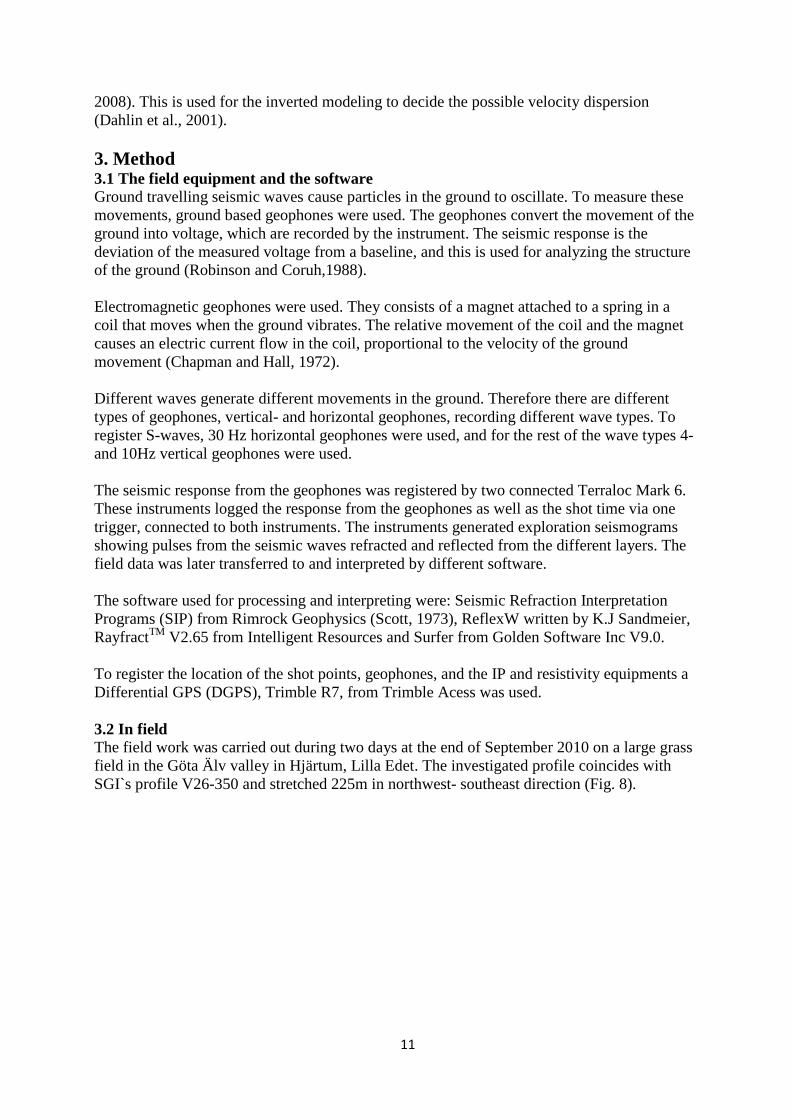
3. Method 3.1 The field equipment and the software

Ground travelling seismic waves cause particles in the ground to oscillate. To measure these

movements, ground based geophones were used. The geophones convert the movement of the

ground into voltage, which are recorded by the instrument. The seismic response is the

deviation of the measured voltage from a baseline, and this is used for analyzing the structure

of the ground (Robinson and Coruh,1988).

Electromagnetic geophones were used. They consists of a magnet attached to a spring in a

coil that moves when the ground vibrates. The relative movement of the coil and the magnet

causes an electric current flow in the coil, proportional to the velocity of the ground

movement (Chapman and Hall, 1972).

Different waves generate different movements in the ground. Therefore there are different

types of geophones, vertical- and horizontal geophones, recording different wave types. To

register S-waves, 30 Hz horizontal geophones were used, and for the rest of the wave types 4-

and 10Hz vertical geophones were used.

The seismic response from the geophones was registered by two connected Terraloc Mark 6.

These instruments logged the response from the geophones as well as the shot time via one

trigger, connected to both instruments. The instruments generated exploration seismograms

showing pulses from the seismic waves refracted and reflected from the different layers. The

field data was later transferred to and interpreted by different software.

The software used for processing and interpreting were: Seismic Refraction Interpretation

Programs (SIP) from Rimrock Geophysics (Scott, 1973), ReflexW written by K.J Sandmeier,

RayfractTM

V2.65 from Intelligent Resources and Surfer from Golden Software Inc V9.0.

To register the location of the shot points, geophones, and the IP and resistivity equipments a

Differential GPS (DGPS), Trimble R7, from Trimble Acess was used.

3.2 In field

The field work was carried out during two days at the end of September 2010 on a large grass

field in the Göta Älv valley in Hjärtum, Lilla Edet. The investigated profile coincides with

SGI`s profile V26-350 and stretched 225m in northwest- southeast direction (Fig. 8).

12

Fig 8. The red line in the left image presents the survey profile. The two images to the right are photos from

field viewing the line seen from the eastern ends and the western ends.

The seismic data gathering was done with two connected ABEM Terraloc Mark 6 (Fig. 9)

with a set-up of 46 channels spacing 5m between geophones with geophone number 1 in the

west and number 46 in the east, located closest to the water. Traditional 48 channels were

used, but since two of the outlet was broken, only 46 channels were used in this survey.

Fig 9. The two connected ABEM Terraloc Mark 6

used in field.

P-wave refraction and reflection seismic data were measured and gathered during day one.

Geophone number 1- 24 were 4Hz and the remaining 10Hz vertical geophones. This data set

was recorded with a sample interval of 1ms in a time window of 800ms. Explosives used as

the energy source were Minex eco, 100g charges for all shots except for the two middle shots

which were charged with 50g. The ignition system was the Nonel, DynoNobel system with U-

475 milliseconds delay.

The geophone and shot points arrangement are seen in Figs. 10 and 11. Two shots were

discharged as far away from the outer most geophones as possible, -36m in the west and 74m

in the water in the east. In addition, two blasts were made 7.5m offset from the outermost

geophones. All charges were drilled down 0.8m, with an offset 1m from the cable. The total

amount of shot points were 27, spread equally along the profile every tenth meter (except

from the two outer most shot points (Fig. 11)).

13

Fig 10. An overview of all the survey profiles made in field.

Fig 11. The relative positioning of the geophones and different shot points for the seismic measurements.

As the cable, geophones and Terralocs were lined out and connected, the measurement

started. The dynamite was placed in the ground and discharged, one at the time and the

geophones collected data from the vibrating ground. The data were viewed and stored in the

Terralocs Mark 6.

Fig 12. An image from one of the black gunpowder blasting in field (Martin Persson, 2010).

Surface wave data, S-wave refraction data and resistivity- and IP- data were collected during

the second day. The used energy source for surface waves was about 200g black gunpowder

filled in plastic bottles dug down in every third hole from the previous day`s blasting. The

trigger worked for all except one which was redone with dynamite. This data set was recorded

with a sample interval of 0.5ms in a time window of 4s with 8192 samples. The data were

collected in the same way as the day before. Before the S-wave refraction measurement

started, all the vertical geophones were changed to 30Hz horizontal geophones. A charge was

14

dug down every 40m (with exception for the 7.5m offset charges), making it totally nine

shots. This data set was recorded with a sample interval of 0.1ms in a time window of 800ms

with 8192 samples. At the same time as the refraction and surface wave data were collected a

resistivity- and IP-data gathering was done.

3.3 DGPS

All shot points, geophones, and resistivity points were registered with a DGPS to coordinate

the survey profile. The data was gathered in post processing format meaning it had to be

corrected afterwards. This was done in the software Trimble Business Center (TBC) where

the survey coordinates were corrected to the data from the fixed station in Onsala, both with

1s data and 30s data to see how much it differed in precision between the two sampling

intervals. In the field, the sampling time was 10s on each point. Since the sampling time only

was 10s the correction with 30s data did not work due to their samplings interval not always

was done in the correction 30s window (It is noteworthy that where the 10s sampling did

correspond to the correction 30s window “new” corrected data correspond with the corrected

1s data). To correct the data, the survey data and the Onsala data were imported to TBC

where baselines were created. The baselines were processed and the survey coordinates were

corrected to the real coordinates using formulas that moved the points to their real locations

corrected by the known location of the fixed points in Onsala.

3.4 Identifying the first arrival time

Due to the quality of the data the two methods P-wave refraction and S-wave refraction were

chosen to be processed in this thesis. The programs used for processing the data were; SIP,

ReflexW, Rayfract and Surfer. First thing to do was to identify the times for first arriving

wave. The first arriving time equals the first registered wave at each geophone. This is a

subjective procedure and has to be done with highest possible accuracy because all the

remaining work of the modeling is based on this. Two programs were used for identifying the

first arrival time; SIP and ReflexW.

The time of the first arriving P-wave was more easily identified compared to the first S-wave,

but at geophones closest to the shot point even the S-wave data was quite clear. Figure 13

presents how the horizontal geophones used for measuring the S-waves filtered the P-waves.

But at geophones further away from the shot point, the geophones had gathered all the P-

wave data too.

Fig 13. The images show the times of arriving waves from one shot where timescale is on the Y-axis and spacing

in meters on the X-axis. In the left image the data was gathered with vertical geophones. The right image

presents the data gathered with horizontal geophones, illustrating how these geophones do not respond to the

first arriving P-waves. Shot point is positioned 36m from geophone 1.

3.5 Modeling in SIP

SIP is an old DOS software consisting of several different modules, such as ASIPIK, SIPIN,

and SIPEDIT. It is an inversion program used for calculating velocities and creating depth and

15

layer models. Here it was used to compare the depth of layers and the velocities with the

ReflexW models since the calculations in this program are more easily understood than the

ones in ReflexW. For modeling in SIP, a maximum of 7 pickfiles (files with times of first

arrivals per shot) could be imported and those were chosen to equally spread along the profile.

Also an elevation file was imported so the program could correct the first arriving times after

the changes in elevation of the geophones (ground surface). The layer affinities were set in the

time-distance graph and the velocity for all layers and locations were calculated, both by

regression of datum-corrected arrivals and by Hobson-Overton method.

With that done, the depths of the layers directly beneath each geophone and shot point were

computed and corrected to surface elevation. In the created model, the SGI data were inserted

and the average velocity for each layer is viewed in the final model presented in chapter 4,

Results and interpretations.

One restriction in the model is the fact that it is based on the identification of the first arriving

wave which was done by hand. Only the P-wave data were processed in SIP for velocity and

depth comparison, due to the unrealistic models from the S-data in the other programs.

3.6 Modeling in ReflexW In contrast to SIP, ReflexW uses spatial interpolation to calculate the layer velocities for

creating the model. The workflow in ReflexW started by identifying the time for first arrived

waves, followed by identifying the interfaces in layershow and modeling the depth and

velocities (see Fig. 14 for the steps).

Fig 14. The images present the different steps in the work flow in ReflexW. Upper image to left shows the

arriving waves from which the first arrival times were identified. Upper image to the right views the window

where each point got their layer properties. The lower image to the left shows the model created in ReflexW and

the last image present the final fixed model created by both ReflexW and Excel.

The text file imported to ReflexW contained elevation and location for the shot points and

geophones, and also the times of first arrivals. The function “insert shot Zerotraveltimes” was

activated to get a more accurate velocity in the uppermost layer. Then the layer affinities were

assigned. The layer affinities were decided according to the degree of the slope, i.e. the

velocity of the layer. A new layer begins with a change in the slope direction. For the layer

16

affinities see Fig. 15. The offset shots were only used to get the variation in velocity of the

bedrock and were not applicable for creating the depth model.

Figure 15. The layer belongings for S-wave data (left) and P-wave data (right).

An inversion was done for the second layer, where the forward and the reverse shot numbers

define the range for the inversion. Before the inversion started, a combined travel time curve

was generated and the total forward and reverse travel times were shown. These differed

significantly and therefore the function “Balance” was activated. This was done to get the true

balanced travel times for the modeling arithmetic calculation and depth analyses.

Before starting the wave front inversion, the model with the first interpreted layer was chosen

as model file. The inversion was then done, based on the total forward and reverse travel

times, and the new layer boundary were plotted in the model. These steps were done for all

layers, and all layers were allowed five different velocities along the profile. The result is a

four layer model containing velocities and depth for each layer.

3.7 Modeling in Rayfract and Surfer

The input-file for modeling in Rayfract consists of a text file containing the location of the

geophones and the shot numbers, all named as station number. The text file also contains the

times for first arriving waves (identified in SIP and ReflexW), the heights and lateral offsets

of the geophones and shot points, also the depth of the shot point (Example in Table 1).

Table 1. An example of a part of an input file to Rayfract.

Shot nr Shot station receiver station break receiver elev shot elev shot depth offset

1 -6.2 1 0.1255 16.532 20.681 0.8 1

1 -6.2 20 0.302 11.007 20.681 0.8 1

1 -6.2 21 0.3087 10.92 20.681 0.8 1

1 -6.2 22 0.312 10.748 20.681 0.8 1

2 1.5 1 0.0288 16.532 16.326 0.8 1

2 1.5 2 0.0308 16.125 16.326 0.8 1

2 1.5 3 0.0408 15.641 16.326 0.8 1

2 1.5 4 0.0529 15.236 16.326 0.8 1

Rayfract uses tomography to model data from seismic refraction surveying, meaning it uses

gridded inversion techniques to determine the velocity of individually 2D blocks within a

profile. This could therefore in some cases give more accurate models with better resolution

of the velocity structures (Persson, 2010). The software makes an inversion of the first arrival

times to estimate a 2D velocity model based on “Wavepath Eikonal Traveltime” (WET)

tomography (Schuster & Quintus-Bosz, 1993). It produces an eikonal equation and the given

17

time for first arriving wave by the elastic wave-equation; this method is named “smooth

inversion”. This method gives a gradual change between layers even if the layers have a

distinct change in velocity, and is therefore not optimal for the Swedish geology. The

additional method Delta t-V is better because of sharper boundaries (but still with gradual

transitions). When the inversion modeling was done, Rayfract exported a GRIDfile to Surfer

where the model was created and interpreted.

Both the S-wave data and P-wave data were tested with the WET model based on first 1D

smooth inversion as initial model, and then tested with recalculated 1D gradient as initial

model giving higher rock velocities. These models were tested with different numbers of

iterations, varying from 10 to 20, where 10 gives the most valid model according to the depth

to bedrock (Figs. 16 and 17 show the P-wave iteration 10 vs 20). Also WET-models based on

initial models done by the Delta T-v method were processed with both 10 and 20 iterations,

where 10 gave the most realistic velocities.

Fig 16. A smooth gradient image with 10 iteration, P-wave data.

Fig 17. A smooth gradient image with 20 iteration, P-wave data.

18

3.8 SGI data

GIS data, CPT-logs (Cone Penetrating test) and shear strength diagrams were supplied by

SGI. The seismic models were compared with SGI´s data to see how well the depth to the

friction material corresponded. The CPT-logs were used in efforts to explain the differences

in S-wave and P-wave models. Finally the SGI’s data and the coordinate data from the field

sampling were posted in GIS to get an overview of SGI´s data points and this investigation for

comparison.

4. Results and Interpretations 4.1 SGI data

In Fig. 18 the location of the six soundings from SGI are plotted together with this

investigations location for shot points and geophones.

Fig 18. The figure presents the SGI-data together with the position for the geophones and shot points from this

investigation.

The figure is created in ArcGis to show the locations correspondence to the SGI data. Three

of the soundings from SGI coincide with this study’s measured profile. The points U05158

(C), U05159 (C) and U05160 (C) are located at 54, 126 and 190m along the profile, measured

from geophone 1.

In Fig. 19, an overview of SGI`s soundings is shown and a red line is added indicating this

study’s location.

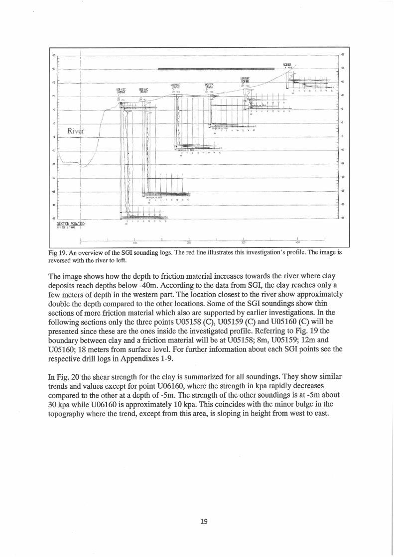
20

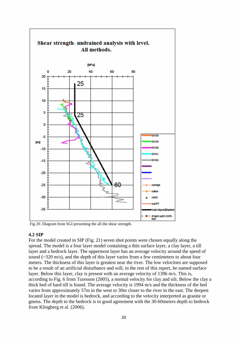
Fig 20. Diagram from SGI presenting the all the shear strength.

4.2 SIP

For the model created in SIP (Fig. 21) seven shot points were chosen equally along the

spread. The model is a four layer model containing a thin surface layer, a clay layer, a till

layer and a bedrock layer. The uppermost layer has an average velocity around the speed of

sound (~320 m/s), and the depth of this layer varies from a few centimeters to about four

meters. The thickness of this layer is greatest near the river. The low velocities are supposed

to be a result of an artificial disturbance and will, in the rest of this report, be named surface

layer. Below this layer, clay is present with an average velocity of 1396 m/s. This is,

according to Fig. 6 from Turesson (2005), a normal velocity for clay and silt. Below the clay a

thick bed of hard till is found. The average velocity is 1994 m/s and the thickness of the bed

varies from approximately 57m in the west to 30m closer to the river in the east. The deepest

located layer in the model is bedrock, and according to the velocity interpreted as granite or

gneiss. The depth to the bedrock is in good agreement with the 30-60meters depth to bedrock

from Klingberg et al. (2006).

22

this stratum is quite homogenous with a velocity around 2000 m/s. This is according to Fig. 6

by Turesson (2005), a normal velocity for till. The layer reaches a thickness of about 60m in

the western part and 30m in the east closer to the river. From the surface, the depth to the

bedrock varies from 60-40m and it slopes from the river. The depth to bedrock is consistent

with the level from earlier investigations by Klingberg et al. (2006), where bedrock is present

at depths of 30-60m beneath surface. The velocity of the bedrock varies from 3800-4800 m/s

with an average velocity of 4262 m/s which according to the velocity table from Turesson

(2005) classifies as granite and gneiss, an expected bedrock type in the area according to

Klingberg et al. (2006).

Fig 22. P-wave model created in ReflexW with added SGI-data shown in black. The average velocity for each

layer is shown in the legend.

The SGI data were added to the model and the depth to friction material seems to correspond

very well. The depth of reconnoiter U05158 coincide in the same way as in the SIP model

where the boundary between clay and till coincide with the first level of SGI´s measured

friction material. According to the sounding log, this first friction layer appears to be only a

half meter thick followed by approximately 3m of clay before new friction material is found.

This sequence is not present in the model. The depth to friction material at the second SGI

point U05159 is about 5m above the boundary in the model, while the depth of U05160 is

similar as the boundary to the model.

4.3.2 S-wave

Like the P-wave model, the S-wave model is a 4 layer model seen in Fig. 23. The uppermost

layer has a low velocity of 91 m/s. This layer is only present in the eastern part of the profile,

from about 140m and eastward. The depth of this layer varies from 0-4m and gets thicker

towards the river. Layer number two has an average velocity of 310 m/s and is therefore

classified as clay. This layer show similar thickness along the entire profile of approximately

20m. The boundary to the underlying layer with an average velocity of 768 m/s is almost

horizontal. This velocity indicate, according to Fig. 6 from Turesson (2005), a layer consisting

of till. The velocities are almost the same in the whole layer, varying between 748-783 m/s.

The till layer is approximately 40-55m thick. The bedrock of either granite or gneiss is located

underneath the layer of till, indicated by the increase in velocity. The average velocity is 1838

m/s with velocity variations between 1500-2000 m/s. Similar to the P-wave model in Fig. 22,

the bedrock slopes towards the western part of the profile, away from the river. The bedrock

in the S-model is located at depths of 65-85m from the surface level.

23

Fig 23. S-wave model created in ReflexW with added SGI-data shown in black. The average velocity for each

layer is shown in the legend.

The depths of clay from SGIs investigation are presented in the model. These depths do not

correspond at all with the model; generally the depths in the S-model are located about 15m

below the SGI depth. The most similar depth is at point U05160 were the difference is

approximately 7m.

4.3.3 Velocity variations in the layers, and boundary trends

When modeling in ReflexW the velocity within each layer were allowed to vary with five

velocities, except from layer 1 where the velocity varies with unknown velocities. In Fig. 24

the variation of the velocity within each layer are presented for both P-wave data and S-wave

data. Except from the surface layer, the velocities of each layer are quite homogenous, and the

velocity differences follow the same trend in bedrock for both S-wave and P-wave.

26

4.4 Rayfract

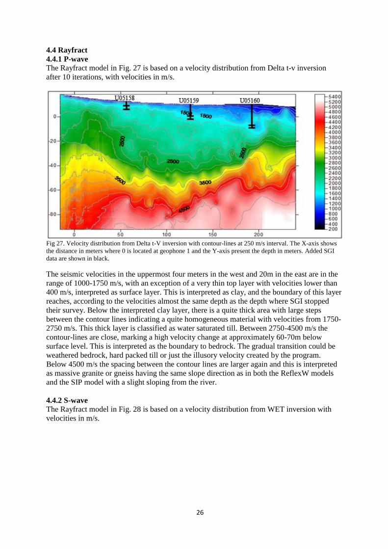
4.4.1 P-wave

The Rayfract model in Fig. 27 is based on a velocity distribution from Delta t-v inversion

after 10 iterations, with velocities in m/s.

Fig 27. Velocity distribution from Delta t-V inversion with contour-lines at 250 m/s interval. The X-axis shows

the distance in meters where 0 is located at geophone 1 and the Y-axis present the depth in meters. Added SGI

data are shown in black.

The seismic velocities in the uppermost four meters in the west and 20m in the east are in the

range of 1000-1750 m/s, with an exception of a very thin top layer with velocities lower than

400 m/s, interpreted as surface layer. This is interpreted as clay, and the boundary of this layer

reaches, according to the velocities almost the same depth as the depth where SGI stopped

their survey. Below the interpreted clay layer, there is a quite thick area with large steps

between the contour lines indicating a quite homogeneous material with velocities from 1750-

2750 m/s. This thick layer is classified as water saturated till. Between 2750-4500 m/s the

contour-lines are close, marking a high velocity change at approximately 60-70m below

surface level. This is interpreted as the boundary to bedrock. The gradual transition could be

weathered bedrock, hard packed till or just the illusory velocity created by the program.

Below 4500 m/s the spacing between the contour lines are larger again and this is interpreted

as massive granite or gneiss having the same slope direction as in both the ReflexW models

and the SIP model with a slight sloping from the river.

4.4.2 S-wave

The Rayfract model in Fig. 28 is based on a velocity distribution from WET inversion with

velocities in m/s.

27

Fig 28. Velocity distribution from a WET inversion with 10 iteration and a Delta t-V inversion model as entrance

model with contour lines at 250 m/s interval. The X-axis shows the distance in meter where 0 is located at

geophone 1 and the Y-axis present the depth in meters. Added SGI data are shown in black.

The seismic velocities in the uppermost 16m varies between 250-400 m/s with an exception

for the area at about X=140m. This location shows a bulge with lower velocities of 0-250 m/s

9m below the surface level. This almost horizontal 250-400 m/s layer is interpreted as clay

and the lower velocities above it, is interpreted as an artificial disturbed surface layer. The

clay-till boundary do not correspond with the depth from SGI soundings at any location.

Below the layer of clay there is a quite homogeneous area with velocities of 400-750 m/s and

a thickness of 20m in the eastern parts, and close to 30m in the western parts. This is

interpreted as till. Below the seismic velocity of 750 m/s the model gets complex and even if

there is a general trend of increased velocity with depth, there are parts in the middle of the

model showing locations with lower velocity below higher velocity locations. According to

this model the bedrock do not seem to appear at all in the eastern parts and in the western the

bedrock could be identified according to the velocity of 2000 m/s in Fig. 6, at depths of 55-

80m below surface level. The complex area between the interpreted till and bedrock layer

could be an area with mixed material after the old landslide shown in Fig. 4. This influence of

a density change would affect the velocities of the S-wave data. It could also be a result of

illusory velocity created by the program as it always creates gradual transitions.

4.5 Depth comparison

In this section the depth to friction material is plotted in diagrams from all the used models, to

get an overview of how well the different models correspond to each other and to the

sounding data from SGI. Note that columns in the diagram always proceed from the sea level

(0), and the outermost point of the column presents the position of depth of the boundary clay

to till, e.g. if the column stops at 5 the boundary is positioned 5m above sea level. This is

mentioned because all the earlier data is presented with the surface level as the reference.

In Fig. 29 the depths modeled at 56m from geophone 1 (where sounding U05158 is located)

are summarized.

29

In this diagram the column “SGI-friction” is not shown due to its value of zero. This location

shows very different results compared to the 56m location. The depth from SIP’s P-wave

model, and both the S-wave and P-wave models from Rayfract agree within 1m compared to

the SGI friction data. The two ReflexW models differ from the SGI depth with 3 and 17m,

respectively. The S-wave model does not coincide with the SGI depth at all. The ReflexW P-

wave depth differed from the depth of the other two P-wave models in Rayfract and SIP with

approximately 5m, contrary to location 56 showing similar results from the three methods.

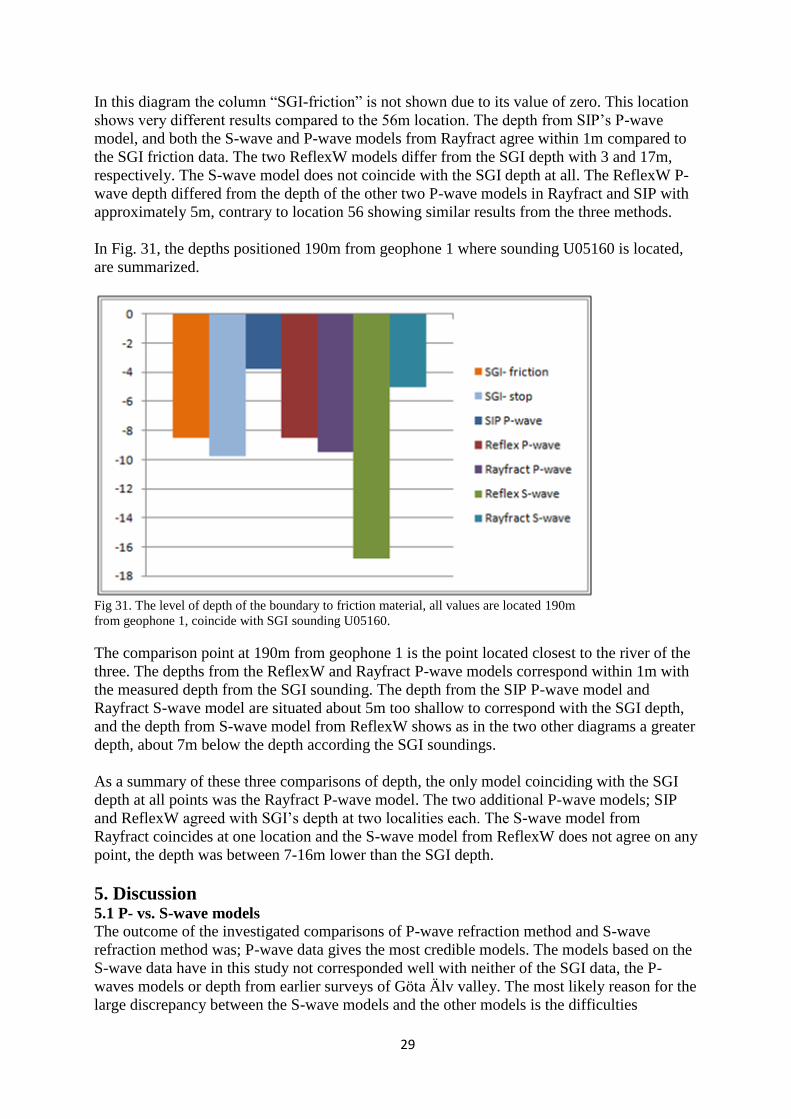
In Fig. 31, the depths positioned 190m from geophone 1 where sounding U05160 is located,

are summarized.

Fig 31. The level of depth of the boundary to friction material, all values are located 190m

from geophone 1, coincide with SGI sounding U05160.

The comparison point at 190m from geophone 1 is the point located closest to the river of the

three. The depths from the ReflexW and Rayfract P-wave models correspond within 1m with

the measured depth from the SGI sounding. The depth from the SIP P-wave model and

Rayfract S-wave model are situated about 5m too shallow to correspond with the SGI depth,

and the depth from S-wave model from ReflexW shows as in the two other diagrams a greater

depth, about 7m below the depth according the SGI soundings.

As a summary of these three comparisons of depth, the only model coinciding with the SGI

depth at all points was the Rayfract P-wave model. The two additional P-wave models; SIP

and ReflexW agreed with SGI’s depth at two localities each. The S-wave model from

Rayfract coincides at one location and the S-wave model from ReflexW does not agree on any

point, the depth was between 7-16m lower than the SGI depth.

5. Discussion 5.1 P- vs. S-wave models

The outcome of the investigated comparisons of P-wave refraction method and S-wave

refraction method was; P-wave data gives the most credible models. The models based on the

S-wave data have in this study not corresponded well with neither of the SGI data, the P-

waves models or depth from earlier surveys of Göta Älv valley. The most likely reason for the

large discrepancy between the S-wave models and the other models is the difficulties

30

regarding identifying first arriving times. It was easier to identify the outermost files and the

ones close to the shooting points, but became more difficult as the distance from the energy

source to the receivers increased. The reasons were the interference of the first arriving S-

wave and the second arriving P-wave, reflexes from P-waves and also possible secondly

generated S-waves from the P-waves. This made the identifying of first arriving S-wave more

of a qualified estimate than knowledge. This might be avoided using a more pointed energy

source.

According to the shape of the till and the bedrock, the S-wave ReflexW model seems to

correspond quite well with both the P-wave models from SIP and ReflexW. The similarity in

shape of the S-wave and the P-wave model from ReflexW could suggest there is something in

the inversion steps that is problematic regarding the depth calculation. But if the differences in

depth would depend only on the spatial interpolation and inversions, the S-wave model from

Rayfract would not correlate with the ReflexW S-wave model as it does.

When comparing the values of velocity changes of each layer, it shows a 28% smaller value

of the clay-till interface for the S-wave compared to the P-wave. This results in a different

refraction angle according to Snell´s law creating greater depths. Small changes in velocity

result in a decrease of the interfaces refraction angle showing greater depths. This because the

wave front spends more time in the ground before the critical angel is reached, and the wave

front returns to surface and are registered at the geophones. But since the velocities are

calculated from the time of the first arriving wave, the source of error still ends up in the

difficulties of identifying first arriving times.

Another reason for the dissimilar depths of the P- and S-wave models could in theory be some

geological features that only affect the S-waves and not the P-waves which would result in

misleading depths. Two factors that S-wave velocities, and not the P-waves depend on, are the

shear strength and the density of the material when situated below ground water table. Since

the survey profile crosses the old landslide, it could be the reason for deviating depth results.

In the S-wave model from Rayfract a lot of inversions are observed as fields of lower

velocities located below higher velocity material. This could reflect layer disturbance and a

mixture of grain size as a result of the landslide. The P-wave data will not detect this, as the

water table is located just below the surface and the velocity is affected by the water

saturation. Looking at the shear strength log from SGI, the data from all the localities follow

the same strength trend except from U05160 at -5m were it loses almost all its shear strength.

According to the formula of S-wave velocity this would be observed by changes in velocity of

the S-wave. This is not the case, and it is not observed in any of the S-wave models.

When comparing the average velocity from the P- and S-wave models, the average general

velocity for the S-wave is almost 1/3 of the P-wave velocity. This is quite low according to

chapter 2.1 where the general differences between P- and S-wave are described as S-wave

velocity is about half the P-wave velocity. This low velocity would result in shallower depths,

which is not the case. The differences regarding the depths in the models decrease with

increase of the actual depth in the measured profile. The shallow part results in greater errors

compared to the deeper parts.

5.2 Bedrock

Since there is no sounding data below the first friction layer there is no actual known depth to

bedrock. However, earlier investigations suggest a depth to bedrock of 30-60m from sea level.

This corresponds with the P-wave models making them more reliable compared to the S-wave

31

models. The depth to the bedrock in all the P-wave models differ less than 10%, which is the

accepted limit for accuracy when using seismic refraction methods (personal communication

with Hegardt and Meland).

All three P-models indicated a bedrock boundary sloping from the river, which is rather

common. Looking at the soil map of the area, a steep high rock unit is located close to the

river on the opposite side, supporting the slope’s direction in the model. The location of the

river is not affected by the shape of the bedrock; the meandering is only affected by the till

and the clay.

5.3 Comparison of the different software models

The depth of the clay deposits from all the created P-wave models correspond quite well with

the SGI depth. Out of the three P-wave models, it was only the Rayfract model that agreed

with SGI’s data at all three compared points. Yet, the depth from Rayfract used for the

comparison is an estimated value from the Rayfract models, and therefore not a precise depth.

Still, it resulted in the most accurate depth compared to the SGI depths, and this is the only

model out of the three P-models that do not depend on human identifying of interfaces and

layer affinities. Rayfract removes one source of error, but the software always creates gradual

velocity changes between interfaces, which not always is the case in the Swedish geology.

The comparison of the accuracy of the different programs used for creating depth models end

up with a higher agreement at greater depth then at shallower depth. One explanation is that

the different calculation and inversion methods used in the different softwares have a greater

impact for small depths than for greater depths. As differences in the calculations get

eliminated with increased velocity, it ends up with a more accurate bedrock depth compared

between models than for example depths to clay.

5.4 The stratigraphy

Common for all the five produced models are the 4 layer models with the same stratigraphy;

artificial disturbed surface layer, clay, till and bedrock. This is the highest resolution of the

stratigraphy the seismic refraction methods could offer in this project. The models do not

show any lenses or layering in the clay, which according to SGI sounding data U05158 is

present with a meter thick deposit of friction material located about 3m above the interface of

clay-till. Instead the models have interpreted this thin lens as the boundary between clay and

till, explained by one of the limitations of the refraction methods, the incapability of detecting

layers with lower velocity below a higher velocity layer. According to earlier investigations in

the area, e.g. Stevens et al. (1990) the stratigraphy consists of different clay layers mixed with

materials of different grain sizes as clay with silt or clay with sand. This resolution is not

present in the produced models, but it is not certain this stratigraphy is present at the site since

the large landslide could have mixed the layers. Therefore, it is possible that the models

present the real stratigraphy with almost homogenous layers. This interpretation is supported

by the varied velocity graphs for each layer, presenting a very small difference in velocity

within each layer, thus indicating homogenous layers with the same grade of consolidation

within the complete layer.

5.5 Till layer

The occurrence of such a thick till layer that all the refraction models present is very rare in

SW Sweden (personnel communication with Stevens). A more likely scenario would be a

glaciofluvium deposit of gravely-sand followed by diamicton (Stevens & Hellgren, 1990).

The gathered resistivity data from the field (Fig. 32) support the boundary of clay- friction

32

material from the refraction models, but it also suggests a more complicated stratigraphy

within the suggested till layer from the refraction models.

Fig 32. A preliminary, uncorrected resistivity image of the profile. No topography was used during inversion,

possible IP-related data are reduced and res2dinvstandardsettings (with robust constraints) are used.

Unpublished.

The interpretation of this resistivity data shall be handled with care since it is uncorrected

preliminary data. However, the model does support the boundary of clay- friction material and

might explain the thick till layer offered by the refraction models. Clay normally has a low

resistivity value, often below 100 Ωm (Dahlin et al., 2001). This boundary in the resistivity

model will therefore support the boundary of the refraction models. A wet gravel and sand

layer normally has a resistivity above 100 Ωm, while a typical coarse-grained Swedish till

often results in a resistivity of several hundred Ωm (Dahlin et al., 2001). The resistivity model

shows varying resistivity values below the clay layer- suggesting a more complex stratigraphy

than the refraction models show. If the refraction data has simplified the stratigraphy of the

layer below the clay to just one layer (interpreted as till according to its velocity) it will affect

the models in the following ways.

The velocity of the layer below the clay is by the software calculated to approximately 2000

m/s in the P-model. If the stratigraphy in reality is more complex hosting several different

layers including some layers like sand and gravel with a much lower velocity compared to the

till, it will affect the depth calculation. If the programs calculate the depth for the unit with

velocity 2000 m/s instead of calculating depth for, say four different units where three of them

has a much lower velocity than 2000 m/s, it will result in an enlarged depth. The program has

the time for the wave spent in ground as well as the velocity; therefore a higher velocity

would lead to greater depths then a low velocity layer with the same arrival time. Referring to

the velocity of till in the refraction models, it probably shows a thin till or another high

velocity layer just below the clay which has “hidden” the low velocity layers below in the

refraction method. Then the real stratigraphy in the “till layer” could be a thin layer of till or

other coarse material followed by sand and gravel and other glaciofluvial deposits as reported

by Stevens and Hellgren, (1990). If there are some hidden layers it also means that the

bedrock probably is displaced and not located as deep as the refraction models suggest

(Mussett and Kahn, 2000). Therefore the till layer would be much thinner and not

homogeneous till. Further work with the resistivity and IP data could give more information

about this and also an interpretation of the reflection data could give a better resolution.

If there is a more complex stratigraphy of the till layer than the refraction data model offers,

with lower velocity layers included it will also affect the slope of the bedrock. Since the

eastern parts of the profile has a much thicker clay layer than the western parts this will

reduce some of the inaccuracy of the depth calculations of the bedrock As the “wrong till

layer” constitute a smaller percent of the material above the bedrock it will have a smaller

33

influence of the total depth than if the clay layer is much thinner as in the western parts. In the

western parts of the profile, the depth of the bedrock almost only depend of the till layer

which lead to greater depths in this area. Therefore, it is possible the bedrock actually slopes

towards the river, instead of from the river suggested by the refraction models.

However, the depth of the bedrock suggested by the refraction data models coincides with the

depth of the bedrock in the river next to the field from earlier studies by Dahlin et al. (2001).

5.6 Surface layer The thin layer of artificial disturbed surface layer with velocities sometimes lower than the

speed of sound has an enormous impact on the depth in the models created in ReflexW. In the

P-model, all the layers were shifted about 15m deeper when not taking this layer into account.

Since there is no surface layer present in the western half of the S-wave model produced in

ReflexW, this could be one of the reasons for the displaced interfaces. The boundary clay-till

slopes towards the river according to the P-wave models and the SGI-data. Therefore it is

possible to assume that the missing surface layer in this part in the S-model could be the

reason of the almost horizontal interface displaced at greater depths. Also the use of the offset

shot points had a great impact on the depth, shifting it downwards, and therefore they were

not used when creating the depth models. They were however used for calculating the

variation of velocity within the bedrock layer.

The low velocity in the upper layer could depend on a pre-trigger at the shot moment, or be a

result of the ribbed surface at the field. The velocity of the artificial disturbed surface layer

could refer to P-wave velocity represented by unsaturated clay or till. This is however

unlikely since the layer is present in the S-wave models. S-waves are not affected by the water

table since they only propagate in solid materials. Irrespective of what this layer really

consists of, it has an impact on the model depths, but was not present in the SGI-data or

observed in field.

5.7 Future work

It would be of interest to do further interpretation of the resistivity and IP-data for comparison

with the clay depths from the refraction models. It would also be of interest to stack the data

to see if the reflection method works, and if it does, to compare those models with the models

from this thesis. One final suggestion for future work in the field would be to redo the surface

wave data gathering with longer time laps.

34

6. Conclusion The field site of this investigation is situated within the scars of an old landslide. The

refraction data results in 4 layer models with material interpreted as artificial disturbed surface

layer, clay, till and bedrock. When comparing depths to the clay-till interface for models from

all methods and the SGI sounding data, the P-wave model from Rayfract offers the best

precision of clay depth compared to the SGI data. Since all the P-wave models end up with

depth to clay within one meter from the SGI depth, this confirms the stop of sounding as the

real boundary to friction material. The bedrock in the models is found at a depth of about 60m

in the western part and 50m in the eastern part of the profile, slightly sloping away from the

river. The differences in depth between the models created with the different softwares

Rayfract, ReflexW and SIP, seem to decrease with depth suggest that the accuracy of the

depth to interfaces increases with the depth. This is suggested to be a result of several hidden

layers in the till layer, affecting the calculations.

The S-wave refraction approach did not offer any reliable models since the depths of the

interfaces were displaced several meters downwards. This is probably a consequence of the

identifying of the time of first arriving wave, and the greater velocity differences between

clay-till layer offered by the S-waves than the P-waves. Therefore the P-wave refraction data

offers the best precisions of soil depth measurements at soil depths greater than 30m. The

velocities in the models suggest homogeneous layers, which can be supported by the old

landslide leaving a homogeneous mixture of the clay. The refraction models did not observe

the approximately 2m thick clay deposit below the one meter sand/gravel lens observed by

SGI sounding in the western parts. This illustrates the limitation of the refraction method in

not detecting too thin layers or lower velocity layers overburden by layers with higher

velocity.

7. Acknowledgement I especially wish to thank my supervisors Erik Meland and PhD Eric Austin Hegardt from

Bergab, and also docent Erik Sturkell for support, offering theoretical help and suggestion,

explanations, help in field, and not least for many interesting and instructive discussions

during the process. They are also thanked for suggestion and work with the thesis and useful

help with the manuscript. PhD student Martin Persson is thanked for his assistance during the

fieldwork and for his useful knowledge of the regional geology and articles about it. Also

Rickard Granqvist is thanked for assistance in field. Birgitta Meland is thanked for lovely

food and accommodation during the field weekend, and Johan Persson is thanked for his

invaluable explanations of Rayfract.

I would also like to thank Hanna Tobiasson Blomen, Mats Öberg and Marius Tremblay on

SGI for their support with their data and for being very helpful with explanations and useful

knowledge. Christian Voelkerling and Leif Utter on Geograf are thanked for assistance and

support with the Trimble problems. Leif Karlsson is being thanked for supporting with the

manuscript correction. Finally Fredrik Schenholm is thanked for being very helpful and

supportive throughout the work with the report writing, and for his patience and support

during the whole project.

35

8. References Books:

Griffiths, D.H., King, R.F., 1981: Applied geophysics for geologists and engineers: the

elements of geophysical. Oxford Pergamont P., 230 pp.

Lindström, M., Lundqvist, J., Lundqvist T., 2000: Sveriges geologi från urtid till nutid. 2:d

edition, Lund studentlitteratur, 530 pp.

Mussett, A.E., Khan, M.A., 2000: Looking into the earth: An introduction to Geological

Geophysics. Cambridge University press, 470 pp.

Parasnis, D:S., 1972: Principles of applied geophysics. 2:d edition. Chapman and Hall, 214

pp.

Reynolds, J.M., 2005: An introduction to applied and environmental geophysics. John Wiley

& Sons, 796 pp.

Robinson, E.S., Coruh, C., 1988: Basic exploration geophysics. John Wiley & Sons, 562 pp.

Sveriges National Atlas 2002: Berg och Jord. 3:d edition, SNA Förlag, 208 pp.

Telford, W.M., Geldart, L.P., Sheriff, R.E., 1990: Applied geophysics. 2:d edition. Cambridge

University press, 770 pp.

Barton Nick, 2007; Rock quality, seismic velocity, attenuation and anisotropy. Taylor and

Francies Group, London, 729 pp.

Reports & Articles:

ABEM Instruction manual, Reference manual for ABEM Terraloc Mk6 v2 and Mk8 with

ABEM SeisTW for Windows XP, 2009.

Dahlin, T., Larsson, R., Leroux, V., Svensson, M., Wisèn, R., 2001: Geofysik i

släntstabilitetsutredningar. Rapport 62, Statens Geotekniska Institut, Linköping, 67 pp.

Järnefors, Björn., 1957; Jordartskarta Götaälvdalen I tre blad, norra bladet. Ser Ba nr 20.

SGU.

Klingberg, F., Påsse, T., Levander, J., 2006: Bottenförhållanden och geologiska utvecklingen i

Göta Älv. SGU rapport K43, 27pp.

Metodblad Ytvågsseismik, Svenska Geotekniska Föreningen. 2008-01-01.

Möller, B., Larsson, R., Bengtsson, P-E., Moritz, L., 2000; Geodynamik i praktiken.

Information 17, Statens geotekniska institut, Linköping. 56 pp.

Persson, J., 2010: Tomografisk modellering med programmet RayfractTM

för bedömning av

bergkvalitè utifrån refractionsseismik. Bachelor of Science thesis B595, Göteborg.

36

Redpath, B.B., 1973: Seismic refraction exploration for engineering site investigations,

Technical Report E-73-4, U.S. Army Engineering Waterways Experiment Station Explosive

Excavation Research Laboratory, Livermore, California

Stevens, R., Hellgren, L-G., 1990; A generalized lithofacies model for glaciomarine and

marine sequences in the Göteborg area, Sweden. GFF, 112: 2, 89- 105

Turesson, A., 2005: Evaluation of combined geophysical methods for characterization of

near-surface sediment. Doctoral thesies A100, Earth Science Centre.

Internet:

Overview of Göta Älv valley Comission, SGI- www.swedgeo.se 2010-09-20

Soilmap from SGU, http://maps.sgu.se/sguinternetmaps/jord/viewer.htm 2010-10-23

Image of Snell`s law, http://galitzin.mines.edu/INTROGP/SEIS/NOTES/snell.gif 2010-09-15

Appendix

ii. Detailed sounding log from SGI, point U05157

iii. Detailed sounding logs from SGI, point U05158 (C)

iv. Detailed sounding logs from SGI, point U05159 (C)

v. Detailed sounding log from SGI, point U05160

vi. Detailed sounding log from SGI, point U05160 C

vii. Detailed sounding log from SGI, point U05161

viii. Detailed sounding log from SGI, point U05161 C

ix. Detailed sounding log from SGI, point U05162

x. Detailed sounding log from SGI, point U05162 C

ii

iii

iv

v

vi

vii

viii

ix

x