14 Week 5 Empirical methods notes

1. Motivation and overview

2. Time series regressions

3. Cross sectional regressions

4. Fama MacBeth

5. Testing factor models.

14.1 Motivation and Overview

1. Expected return, beta model, as in CAPM, Fama-French APT.

1TS regression, define : = + 0 + = 1 2 .

2 Model: () = 0 (+)

(+) because the point of the model is that should = 0.

2. 1 is useful to understand variation over time in a given return, for example, to find good

hedges, reduce variance. 2 is for when we want to understand average returns in relation to

betas (cross section)

3. How do we take this to the data? Objectives:

(a) Estimate parameters. .

(b) Standard errors of parameter estimates. How do vary if you draw new data and

try again?

(c) Test the model. Does () = 0? Are the = 0? Are the that we see due to badluck rather than real failure of the model?

(d) Test one model vs. another. Can we drop a factor, e.g. size?

4. Statistics reminder. There is a true value of , which we don’t know.

(a) We see a sample drawn from this truth, generating estimates , , . These sample

values vary from the truth, but they’re our best guess.

(b) “Standard errors:” If we ran history over and over again, with different luck, how would

the estimates , , vary across these alternative universes. “

(c) Test” If the true alpha (say) were zero, how often (in how many alternate universes)

would we see an alpha as big as the we measure in this sample? If not many it’s

unlikely that the true is zero.

225

14.2 Statistics review

is a random variable (say, stock return) drawn from a distribution with mean and variance 2.

You see a sample , meaning (1 2 ). You do not see the true . Your job is to learnwhat you can about them from the sample.

Estimate

You might firm the sample mean

=1

X=1

as a good guess of the mean. This is the estimate. We don’t have to use this estimate — we could

use the median if we wanted to. If so, we’d get different formulas for what follows.

The sample mean is a number to you. But it is also a random variable — it could have come

out differently. It’s like flipping a coin just once. Quiz: do you really understand the difference

between and ?

Standard error

The standard error of the mean

()

is your best guess of how differently might have come out if you run history all over again. If

you will, it’s your best guess of how much the sample mean varies across all alternative universes

which are just like ours but different luck of the draw.

How can we guess such a thing, given that we only see one ? You can’t take the variance with

a single observation! Answer: with assumptions. Start with

2 () = 2

Ã1

X=1

!=1

2

h2 () + 2( − 1)( −1 +

i(What the...Yes, look at = 3, and remember (1 2) = (2 3) = (3 2) = ( −1),

2 () = 2µ1

3(1 + 2 + 3)

¶=1

9

h32() + 2( −1) + 1( −2)

iNow, let’s add an assumption that the sample is also drawn independently. Then all the cov

terms are zero, and we get the familiar formula

2() =2()

;() =

()√

Make sure you understand this. The standard error of the (sample) mean, your best guess of how

the one sample mean you see would vary if you could run history all over again is related to the

standard deviation of x , how much x varies over time in the one sample you do see. It’s rather

amazing that we can connect these two quantities!

(What if is correlated over time, you ask? Actually, that’s easy to solve. Just use the formula

with all the cov’s in it. This is the “generalized method of moments” formula, which Asset Pricing

explains in great detail. It’s important to recognize: the standard formula √ only works for

that are uncorrelated over time. There is a better formula that corrects for this correlation. As an

226

extreme example, if all the are perfectly correlated, then you’re really seeing one observation not

observations.)

Hypothesis test

The next thing we might want to do is a hypothesis test to characterize our uncertainty about

the true . What we have so far is that is our best guess of the true and () measures our

uncertainty about that guess. The hypothesis test puts that observation another way: suppose you

saw = 10. What is the chance of seeing = 10 or larger, just by chance, if the the true = 0?

To answer that question, let’s add another assumption (not really needed, but easier for now),

that the are normally distributed. Now, we can rely on a theorem from statistics (which is just

algebra) that the sum of normally distributed random variables is also normal. Thus, if the true

values are and , then the sample mean has the distribution

˜³ () =

ë

Equivalently, the sample mean divided by its standard error has a standard normal distribution

−

()=

−

√= ˜ (0 1)

Now you’re ready to do a hypothesis test: If the true value really was zero, form the number

() = ³√´Compare the number you have to the normal (0,1) distribution (table or in

matlab) that tells you the chance of seeing something this big or bigger. (A number of about 2

corresponds to about 2.5% chance of seeing a bigger number.)

A fly in the ointment: What do you use for ? You don’t know that. You could try using your

best guess, the sample standard deviation

2 =1

X( − )2

(or 1( −1), the difference doesn’t matter here. ) Quiz: Do you understand the difference between and ?. Using that guess, you’d form the number

−

√

However, looking across samples, (alternate universes) now varies too, so this number will vary by

more than the last number we created. Fortunately, a smart statistician figured out the distribution

of this number — the sample mean divided by the sample standard deviation. It’s called the

distribution. So we write−

√˜

And you compare the number you create on the left hand side to this distribution, slightly fatter

than the normal, to figure out what the chance is of seeing a this big (10) if the true were zero.

The distribution is exactly correct if the are normal. As rises, the distribution looks

more and more like the normal distribution. The gets close to quickly. Even if the underlying

are not normally distributed, this number still converges to a normal distribution (the “central

limit theorem”).

227

Similarly, statisticians have worked out the distribution of

(− )2

2

If the are normally distributed, this has an distribution. (That’s just a name for a function, the

way “normal distribution” is a name for () = 1√2−

2. The form of the function doesn’t matter,

as your computer has it.) Even if the are not normally distributed, for large this number has

a 2 distribution. This mirrors the facts for the and normal distribution.

Why square it? Squaring it allows you to generalize and do multiple tests together. The basic

idea: suppose and are independent of each other with a standard (0 1) distribution. Then

2 + 2˜22

(read as “chi-squared with two degrees of freedom.”) That just means that statisticians have tab-

ulated the distribution of a sum of two normals.

Here’s how we use that. Suppose and are both iid with mean =h

iand covariance

matrix Σ. Then h − −

i0 µΣ

¶−1 " − −

#has a 22 (chi-squared with two degrees of freedom) distribution for large . If x and y are also

normally distributed then this number has a F distribution, which is exact for any .

14.3 Time-Series Regression

1. Setup: test assets. factors ( = 1 for CAPM, = 3 for FF). time periods. The

factors are also excess returns like rmrf, hml, smb, not real variables like ∆

2. * It’s useful to think of data in vector, matrix format

assets

time

⎡⎢⎢⎢⎢⎣11 21

1

12 22 2

...

1 2

⎤⎥⎥⎥⎥⎦There are -vectors across assets,

=h1 2

i0() =

h1 2

i0and -vectors across factors

=h1 2

i0() =

h(1) (2) ()

i0(I’ll use = 1 wherever possible). Vectors are column vectors.

228

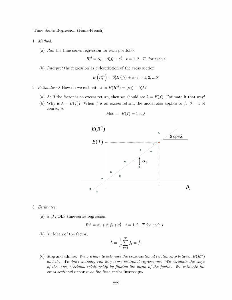
Time Series Regression (Fama-French)

1. Method:

(a) Run the time series regression for each portfolio.

= + 0 + = 1 2 . for each

(b) Interpret the regression as a description of the cross section

³

´= 0 () + = 1 2

2. Estimates: How do we estimate in () = () + 0?

(a) A: If the factor is an excess return, then we should see = (). Estimate it that way!

(b) Why is = ()? When is an excess return, the model also applies to . = 1 of

course, so

Model: () = 1×

i

( )eiE R

Slope

i

1

( )E f

3. Estimates:

(a) : OLS time-series regression.

= + 0 + = 1 2 for each .

(b) : Mean of the factor,

=1

X=1

=

(c) Stop and admire. We are here to estimate the cross-sectional relationship between ()

and . We don’t actually run any cross sectional regressions. We estimate the slope

of the cross-sectional relationship by finding the mean of the factor. We estimate the

cross-sectional error as the time-series intercept.

229

4. Standard errors:

(a) Reminder of the standard error question: There are true parameters which we

don’t know. In our sample, we produce estimates . Due to good or bad luck,

these will be different from true values. If we could rewind and run history over and

over again, we’d get different values of . How much would these vary across the

different samples? If we thought = 0, how likely is it that the we see is just due to

luck? To answer these questions we need to know what () ³´ ³´are. Watch

it — this is how much the estimates would vary across “alternate universes”. These

quantities are called standard errors.

(b) Suppose are independent over time. For each asset, (+) = 0. I do not assume

( ) = 0 — that would be a big mistake — returns are correlated with each other at a

point in time!

(c) ⇒(statistics) Then you can use OLS standard errors .(d) ⇒(statistics) For , our old friend: If are uncorrelated over time,

() =()√

Applying it to ,

() =()√

5. Test

(a) Reminder of t statistic. () = . This shouldn’t be too big if the true alpha is zero.

“due to luck” it will only be over 2 in 5% of the samples.

(b) We want to know if all are jointly zero. We know how to do () (), () −−from the i and jth time series regression — but how do you test all the together?

(c) Answer: look at

0( 0)−1

This is a number. If the true is zero, this should not be “too big.” Precise forms,

0()−1 = h1 + 0Σ−1

i−10Σ−1˜2

− −

h1 + 0Σ−1

i−10Σ−1˜−−

GOAL: Understand use this formula, know where to look it up. Not memorize or derive

it!

(d) “˜” means “is distributed as,” meaning the number of the left follows the distribution

given on the right. Procedure: compute the number on the left. Compare that number

to the distribution on the right, which tells you how likely it is to see a number this large,

if the true are all zero. (Note = number of factors only; i.e. 1 for the CAPM. Don’t

add another K for the constant. Also the F test wants you to use 1 in computing the

covariance matrices. )

230

(e) Conceptually, it’s just like a t test,

()˜;

2

()2˜2 ,

You compute the number on the left, and compare to the t distribution on the right. If

the number is bigger than 2, you say there is less than 5% chance of seeing a number

this big if the true x is zero. Our test is just the vector version of the squared t test —

estimate divided by standard error.

(f) What is all this stuff?

i. = all the intercepts together.

=

⎡⎢⎢⎢⎣12

⎤⎥⎥⎥⎦ii. Σ = covariance matrix of regression residuals.

Σ =

⎡⎢⎢⎢⎢⎣2(1) (12) (1 )

(12) 2(2) (2 ). . .

2()

⎤⎥⎥⎥⎥⎦

=

⎡⎢⎢⎣1

P=1

21

1

P=1 12

1

P=1 12

1

P=1

22

. . .

⎤⎥⎥⎦Most simply,

=

⎡⎢⎢⎢⎣12

⎤⎥⎥⎥⎦Σ = (

0)

Σ is not diagonal. Returns and residuals are typically correlated across assets even

if not over time. (1 1−) = 0, but (1

2 ) 6= 0. (Industry, other nonpriced

factors).

iii. 0Σ−1 is a number. (See “quadratic form” in the matrix notes)iv. = mean of the factors (); Σ = covariance matrix of the factors. .For CAPM,

= ();Σ = 2()

For FF3F,

=

⎡⎢⎣ ()

()

()

⎤⎥⎦

Σ =

⎡⎢⎣ 2() ( ) ( )

( ) 2() ( )

( ) ( ) 2()

⎤⎥⎦

231

v.h1 + 0Σ−1

iis a number.

vi. Why isn’t this in regression class? We are running regressions side by side and

asking for the joint distribution of coefficients across regressions. In regression class,

you only run regressions one at a time.

(g) Interpreting the formula

i. Even if the true = 0, we will see 6= 0 in sample. Firm may get lucky, have a

high average return in sample. But should not be “too large.”

ii. Negative is as bad as positive.

iii. We want one number to summarize if the are, on average, “too big.” How about

the sum of squared ?

21 + 22 + + 2 = 0

0 =h1 2

i⎡⎢⎢⎢⎣12

⎤⎥⎥⎥⎦iv.

0( 0)−1

is a weighted sum of squares. For example, if ( 0) is diagonal,

h1 2

i⎡⎢⎢⎢⎢⎣−21

−22. . .

−2

⎤⎥⎥⎥⎥⎦⎡⎢⎢⎢⎢⎣

12...

⎤⎥⎥⎥⎥⎦

h1 2

i⎡⎢⎢⎢⎢⎢⎢⎣

121222...

2

⎤⎥⎥⎥⎥⎥⎥⎦=

Ã2121+

2222+ +

22

!

This pays more attention to alphas corresponding to assets with low . Those are

better measured. For example, if = 0, then is perfectly measured — we should

really pay attention to that one, and reject the model if it is even 0.00000001!

v. Fact:

( 0) =1

h1 +()0Σ−1 ()

iΣ

Thus our statistics are based on the size of

0( 0)−1

vi. If the are really zero, will not be zero due to luck, and 0( 0)−1 0.

How large will 0( 0)−1 typically be? How often should we see 3? 5?

232

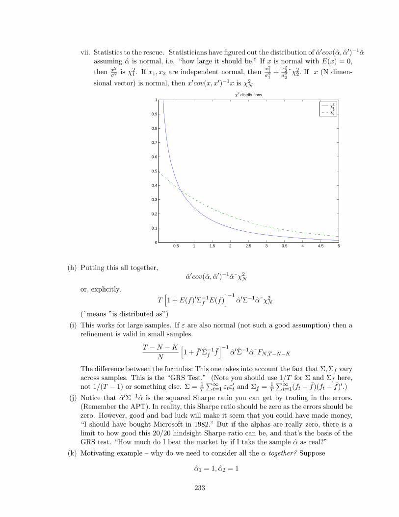
vii. Statistics to the rescue. Statisticians have figured out the distribution of 0( 0)−1assuming is normal, i.e. “how large it should be.” If is normal with () = 0,

then 2

2is 21. If 1 2 are independent normal, then

2121+

2222˜22 If (N dimen-

sional vector) is normal, then 0( 0)−1 is 2

0.5 1 1.5 2 2.5 3 3.5 4 4.5 50

0.1

0.2

0.3

0.4

0.5

0.6

0.7

0.8

0.9

1χ2 distributions

χ21

χ22

(h) Putting this all together,

0( 0)−1˜2or, explicitly,

h1 +()0Σ−1 ()

i−10Σ−1˜2

(˜means ”is distributed as”)

(i) This works for large samples. If are also normal (not such a good assumption) then a

refinement is valid in small samples.

− −

h1 + 0Σ−1

i−10Σ−1˜−−

The difference between the formulas: This one takes into account the fact that ΣΣ vary

across samples. This is the “GRS Test.” (Note you should use 1 for Σ and Σ here,

not 1( − 1) or something else. Σ = 1

P∞=1

0 and Σ =

1

P∞=1( − )( − )0)

(j) Notice that 0Σ−1 is the squared Sharpe ratio you can get by trading in the errors.(Remember the APT). In reality, this Sharpe ratio should be zero as the errors should be

zero. However, good and bad luck will make it seem that you could have made money,

“I should have bought Microsoft in 1982.” But if the alphas are really zero, there is a

limit to how good this 20/20 hindsight Sharpe ratio can be, and that’s the basis of the

GRS test. “How much do I beat the market by if I take the sample as real?”

(k) Motivating example — why do we need to consider all the together? Suppose

1 = 1 2 = 1

233

and

(1) = (2) = 1

Then

=

()= 1

so each alone is not significant. Is the model right? Maybe the alpha of a equal weight

portfolio of the two assets is significant? 1 + 2 is significant? Let’s check. The for

1 + 2 is

=1 + 2

(1 + 2)

Now,

2(1 + 2) = 2(1) + 2(2) + 2(1 2)

Suppose

(1 2) = −09Then

2(1 + 2) = 1 + 1− 2× 09 = 02(1 + 2) =

√02 = 044

=1 + 2

(1 + 2)=

2

044= 454

This is significant.

(l) What happened? The model can be rejected for the portfolio 1 + 2 even though

not for the individual assets. This portfolio alpha is much better measured than the

individual because of the negative covariance. If we had done the initial test on

the portfolio 1 + 2 rather than on the two separately, we would have gotten a

rejection. We don’t want our test to depend on which portfolios we happen to choose!

The test looks over all possible portfolios and makes sure we don’t miss even the worst

one. This portfolio also has a lot less variance. Well, standard error is √ , so the

minimum-variance portfolios are the best measured ones.

(m) Why do we need a new formula? Why wasn’t this in regression class? Answer: In

regression class, you learned how to do the standard errors of a single regression,

= + + ,for one i at a time. You learned “joint” distributions and tests

like and together. “Joint” meat multiple right hand variables with a single left

hand variable. Here we are running multiple regressions — many left hand variables —

next to each other. We need to think about the joint distribution of and when

we’re running two regressions at a time. Econometrics books just never thought of doing

that. The methods and formulas are exactly the same as in your OLS regression classes

though, once we ask that new question.

6. BIG PICTURE: We have a procedure for estimating the parameters , for standard

errors (), (), () and a test for “are all = 0” based on the idea that the sum of

squared should not be “too big.”

7. Read Fama and French, “Multifactor Anomalies” p. 57 last paragraph, “the F test of...” This

is what they’re talking about! High 2 means small Σ so small are “significant.”

234

8. All these statistics, and especially the GRS test, are derived from the classical assumptions

that returns are independent over time, correlated across assets, and (for finite sample results)

normally distributed. There are more modern formulas that account for correlation of asset

returns over time, conditional heteroskedasticity (returns are more volatile at some times

than others) and non-normality. They aren’t that hard — they’re all instances of GMM. Asset

Pricing explains in detail. Though people should use these formulas, they largely don’t, alas.

14.4 Cross-sectional regression

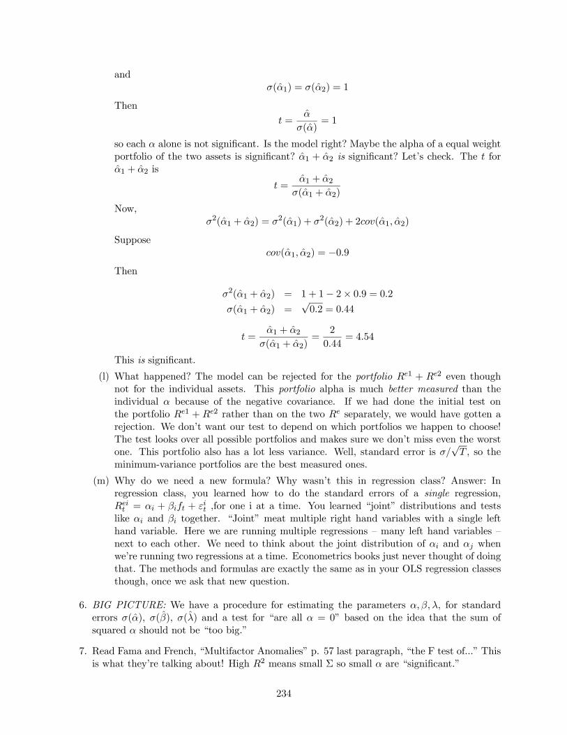
1. Another idea. The main point of the model is to understand average returns across assets,

i

( )iE R

Slope

i

() = 0 (+) = 1 2

Why not fit this as a cross sectional regression, rather than just infer from the factor mean?

(More motivation, and time -series vs. cross section comparison at the end.)

2. Method: This is a two step procedure

(a) Run TS (over time for each asset) to get ,

= + + = 1 2 for each .

( not .Let’s reserve for the pricing error () = + , and it’s not clear yet

what will be. )

(b) Run CS (across assets) to get .

() = () + + = 1 2

is optional.

3. Don’t get confused. () is the variable. is the variable. is the slope (not ). is the error term. (Potential confusion: , the intercept of the time series regression, is the

error of the cross-sectional regression.)

4. Estimates:

235

(a) from TS.

(b) slope coefficient in CS.

(c) from error in CS: = 1

³P=1

´− 6= is not the intercept from the time

series regression any more.

5. Standard errors.

(a) () from TS, OLS regression formulas.

(b) (). With no intercept in CS,

2() =1

h¡0

¢−10Σ(0)−1

³1 + 0Σ−1

´+Σ

i(c) ()

() =1

³ − (0)−10

´Σ³ − (0)−10

´³1 + 0Σ−1

´(d) Yuk yuk yuk... why is this so bad?

i. The usual regression is = + . The standard error formulas assume the are not correlated with each other. Our regression is () = + . The are correlated with each other. If Ford has an unluckily low alpha, then GM is

also likely to have an unluckily low alpha. We need standard errors that correct for

correlation across assets.

ii. This is a pervasive problem, so important to think about. Most regressions you

run in finance have this problem. Corporate example: does investment respond to

market values or to profits (“internal cash”)?

investment = + × Book/Market + × profits +

Whatever other shocks make Ford likely to invest more, also probably affect

GM. Fama’s rule: standard errors and t statistics that don’t correct for this are off

by about a factor of 10.

iii. We also need to correct for the fact that are also estimated, in the same sample.

(e) Now, look at the formula. It’s really not that bad.

i. Ingredient #1. Before we had 2() = 2³1

P=1

´= Σ . We have that again!

(Last term)

ii. Ingredient #2. Run a classic regression with correlated errors. (OLS regression with

correlated errors, not GLS regression.)

= + ; ( 0) = Ω = ( 0)−1 0 = ( 0)−1 0 (+ )

() = ! (unbiased)

2() = h( 0)−1 0 0( 0)−1

i= ( 0)−1 0Ω( 0)−1

That’s just what we have, with = (remember, are right hand variables!).

236

iii. This is a really useful tool! It’s the basis for “clustered standard errors” and other

ways to correct standard errors for correlation.

iv. Similarly, cov() formula is also the classic regression formula for covariance of the

residuals ( are errors in the CS regression) For math nerds who really want to see

it:

= −

= −( 0)−1 0

=³ −( 0)−1 0

´

=³ −( 0)−1 0

´( + )

() =³ −( 0)−1 0

´

=³ −( 0)−1 0

´ = 0

( 0) = h³ −( 0)−1 0

´ 0

³ − 0( 0)−1

´i=

³ −( 0)−1 0

´Ω³ − 0( 0)−1

´(f) Yucky formulas, but look them up when you need them. Point: understand them well

enough to look them up and calculate them.

(g) With an intercept , (() = + +) we need () too. This will work just like

OLS with a constant Let

=

⎡⎢⎣ 1 |1

1 |

⎤⎥⎦i.e the right hand variables in the cross sectional regression. Then,

2

Ã"

#!=1

"¡ 0

¢−1 0Σ( 0)−1

³1 + 0Σ−1

´+

"0 0

0 Σ

##

() =1

³ −( 0)−1 0

´Σ³ −( 0)−1 0

´ ³1 + 0Σ−1

´6. Test

0( 0)−1˜2−−1

7. Point: understand the question these formulas are answering, a bit of why they look so bad

(and why OLS formulas are wrong/inadequate.) Know where to go look them up.

14.5 Fama - MacBeth procedure.

1. A relative of cross - sectional regression.

2. Procedure, applied to asset pricing models:

237

(a) Run TS to get betas.

= + 0 + = 1 2 for each .

(b) Run a cross sectional regression at each time period,

= 0 + = 1 2 for each

(Again, is the and is the slope. You can add a constant if you want.

= + 0 + = 1 2 for each

(c) Then, estimates of are the averages across time

=1

X=1

; =1

X=1

(d) Standard errors use our friend 2() = 2() (Assumes uncorrelated over time — ok

for returns but not for many other uses!)

2() =1

() =

1

2

X=1

³ −

´2() =

1

() =

1

2

X=1

( − ) ( − )

This one main point. These standard errors are easy to calculate. Back in 1972, we

didn’t have the huge formulas above, and this was the only way. Now you can do it

either way. It’s a mind blowing idea — use √ applied to the monthly cs regression

coefficients! But it works.

(e) Test

0( 0)−1˜2−1

3. Intuition: To assess () you could split sample in half. Or in quarters? ... Or go all the way.

4. Fact: If the are the same over time, the FMB estimates are identical to the cross-sectional

regression. The CS standard error formulas are just a little bit better (they include error of

estimating ), but the difference is very small in practice.

5. One advantage of FMB: it’s easy to do models in which the betas change over time. That’s

harder to incorporate in time-series and cross-sectional regressions. (Still it’s perfectly possi-

ble)

6. Other applications of Fama-MacBeth: any time you have a big cross-section, which may be

correlated with each other. (If the errors are uncorrelated across time and space, just stack

it up to a huge OLS regression, as on the problem set)

(a)

+1 = + ln + ln + +1

This is an obvious candidate, since the errors are correlated across stocks but not across

time. FF used FMB regressions in the second paper we read.

238

(b) Corporate finance does this all the time.

investment = + × Book/Market + × profits +

(c) You can’t just stack it all up and run a big OLS regression. Well, you can — the estimates

are ok — but you can’t use the standard errors, because the are correlated with each

other. Think of the limit that the are all the same. Now you really have data points,

not × data points. FMB is one way to correct the standard errors. “Clustering”

which is like the cross-sectional regression formulas above is another.

(d) This is a big deal in a recent survey Kellogg’s Mitch Petersen found that more than

half of all published papers in the journal of finance ignored the fact, and that standard

errors are typically off by a factor of 10. Half the stuff in the JF is wrong!

14.6 Testing one model vs. another

1. Example. FF3F.

() = + + +

Do we really need the size factor? Or can we write

() = + +

and do as well? ( will rise, but will they rise “much”)

2. A common misconception: Measure = (). If = 0 (and “small”) we can drop

it. Why is this wrong? Because if you drop from the regression, and also change!

(a) Example 2: CAPM works well for size portfolios, but shows up in FF model

() = 0 + ← works, higher with higher ()

() = 0 + + ← works too, all = 1 and 0

(b) Example 3. Suppose the CAPM is right, but you try a “Microsoft” factor.

() = () + (

)

() = 0 so it looks like we need the new factor!

(c) Example 4: Suppose

=1

2 +

1

2

Now, obviously, we can drop as a factor. But just as obviously, = () =12 () +

12 () 0.

3. Reminder: Multiple regression coefficients don’t change if right hand variables are not corre-

lated. Conclusion: = 0 would be right if rmrf, hml, smb were not correlated. They are

correlated alas.

(a) In my example, 0 and correlation of microsoft with the market was crucial. In

example 4, you can see the correlation of smb and the other factors.

239

(b) If we orthogonalize the right hand variables

= +

+

= +

+ (

−

) +

³

´= + (

) + (

−

)

“Ortholgonalize” means that by construction and (

− ) are uncorrelated. In

this case it’s clear that the CAPM holds if the mean of the new factor = −

is zero.

4. Solution:

(a) “ First run a regression of on and and take the residual,

= + + +

Now, we can drop smb from the three factor model if and only is zero. Intuitively,

if the other assets are enough to price smb, then they are enough to price anything that

smb prices.

(b) “Drop smb” means the 25 portfolio alphas are the same with or without smb

(c) *Equivalently, we are forming an “orthogonalized factor”

∗ = + = − −

This is a version of smb purged of its correlation with rmrf and hml. Now it is ok to

drop if (∗) is zero, because the and are not affected if you drop ∗

(d) *Why does this work? Think about rewriting the original model in terms of ∗,

= + + + +

= + ( + ) + ( + ) + ( − − ) +

= + ( + ) + ( + ) + ∗ +

The other factors would now get the betas that were assigned to smb merely because

smb was correlated with the other factors. This part of the smb premium can be captured

by the other factors, we don’t need smb to do it. The only part that we need smb for is the

last part. Thus average returns can be explained without smb if and only if (∗) = 0

5. *Other solutions (equivalent)

(a) Drop smb, redo, test if 0()−1 rises “too much.”

(b) Express the model as = − 1 − 2 − 3, 0 = (). A test on is

a test of “can you drop the extra factor.”

6. Why do FF keep smb?

(a) Because they want a good factor “model of returns and average returns.” Smb can be

very useful to explain variance even if its addition does not help to explain means.

240

(b) Because adding smb reduces () and Σ, making all measurements better and standard

errors smaller

(c) Example: Suppose 2 = 100% in the time series regression with smb, but 90% without

it. Then knowing that all your test assets are different portfolios of smb, and all their

pricing comes down to arbitrage pricing with smb is very useful!

(d) Moral: what factors you want to use depends on what you want to use the model for!

14.7 Time series vs. cross section

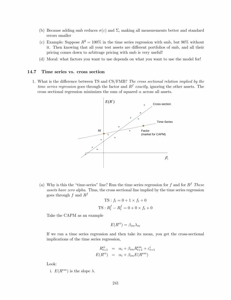
1. What is the difference between TS and CS/FMB? The cross sectional relation implied by the

time series regression goes through the factor and exactly, ignoring the other assets. The

cross sectional regression minimizes the sum of squared across all assets.

i

( )iE R

Time-Series

Cross-section

Factor(market for CAPM)

Rf

(a) Why is this the “time-series” line? Run the time series regression for and for These

assets have zero alpha. Thus, the cross sectional line implied by the time series regression

goes through and

TS : = 0 + 1× + 0

TS : −

= 0 + 0× + 0

Take the CAPM as an example

() =

If we run a time series regression and then take its mean, you get the cross-sectional

implications of the time series regression,

+1 = +

+1 + +1

() = + ()

Look:

i. () is the slope .

241

ii. , the intercept of the time series regression is now the error of the cross-sectional

relation

iii. This cross-sectional line goes right the Rf and Rm with zero alpha; () =

0 + 1×() and = − has 0 = 0 + 0×()

(b) Issue 1: do you want to estimate the factor risk premium from the mean of the factor,

or to best fit the cross section of returns?

(c) Issue 2: Do you want to force the intercept to go through the risk-free rate? (Run cross-

section regression with or without free constant )

(d) Equivalent: Do you want to set = 0 for the market and riskfree, or accept some bigger

there to make other small?

(e) Note: for a good model, it shouldn’t really matter.

(f) “Right answer?” Sorry! Econometrics is a lot of tools and you have to use judgement!

2. Why might you use a cross-sectional regression? Art!

(a) It’s closer to heart of the asset pricing model. “Average returns are higher if beta is

higher.”

(b) It’s useful to add characteristics and test if they are zero.

() = () + + () + () + (2 ) + = 1 2

should be zero. Do betas drive out characteristics?

(c) Fact: If the model is absolutely right, if the factor is an excess return (like CAPM,

FF3F), the market proxy is perfect, if the interest rate proxy is the real risk free rate,

and if returns are normally distributed, the time series regression (run the CAPM line

through and , ignore other assets; = () = (), etc. ) is

statistically optimal.

(d) *Fact: The time series regression is exactly the same as a generalized least squares GLS

estimate of the cross sectional regression. =¡0Σ−1

¢−10Σ−1(). Σ = 0

for the factors and risk free rate, since there is no error in their time-series regressions.

(Same fact, GLS is statistically optimal)

Why should you ignore all the information in the other alphas?

= + +

() has no extra information about () that does not already have. The same

measurement plus error does not refine a measurement.

(e) But... Advice 1: when models are not perfect, it’s often a good idea to run OLS (with

correct standard errors) rather than “statistically optimal” GLS. Here: is your market

proxy the real wealth portfolio? Do people borrow and lend freely at the 3 month T bill

rate? Etc.

(f) But... betas are not perfectly measured. Mis-measured right hand variables leads to

“too flat” regression lines (“downward bias”) — just what we see. = 1 on market is

perfectly measured!

242

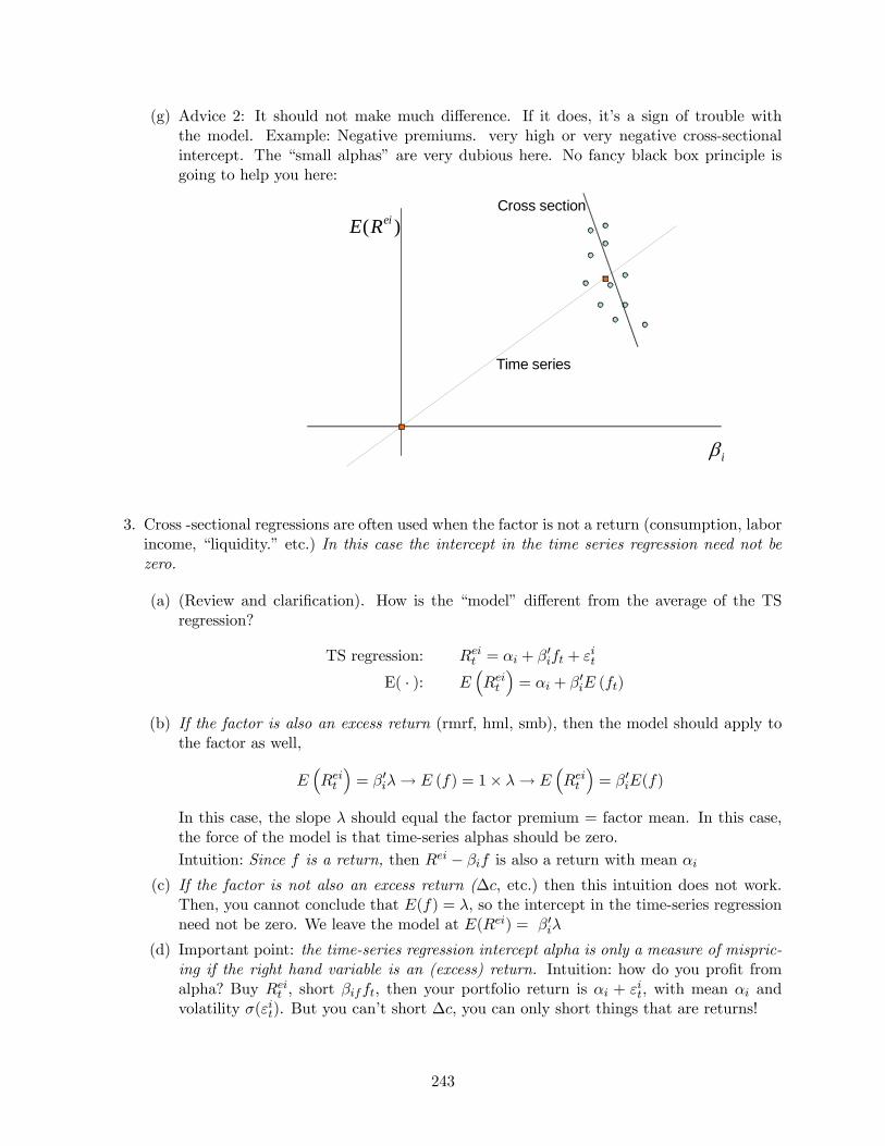
(g) Advice 2: It should not make much difference. If it does, it’s a sign of trouble with

the model. Example: Negative premiums. very high or very negative cross-sectional

intercept. The “small alphas” are very dubious here. No fancy black box principle is

going to help you here:

i

( )eiE R

Time series

Cross section

3. Cross -sectional regressions are often used when the factor is not a return (consumption, labor

income, “liquidity.” etc.) In this case the intercept in the time series regression need not be

zero.

(a) (Review and clarification). How is the “model” different from the average of the TS

regression?

TS regression: = + 0 +

E( · ): ³

´= + 0 ()

(b) If the factor is also an excess return (rmrf, hml, smb), then the model should apply to

the factor as well,

³

´= 0→ () = 1× →

³

´= 0()

In this case, the slope should equal the factor premium = factor mean. In this case,

the force of the model is that time-series alphas should be zero.

Intuition: Since is a return, then − is also a return with mean

(c) If the factor is not also an excess return (∆, etc.) then this intuition does not work.

Then, you cannot conclude that () = , so the intercept in the time-series regression

need not be zero. We leave the model at () = 0

(d) Important point: the time-series regression intercept alpha is only a measure of mispric-

ing if the right hand variable is an (excess) return. Intuition: how do you profit from

alpha? Buy , short , then your portfolio return is + , with mean and

volatility (). But you can’t short ∆, you can only short things that are returns!

243

(e) *Technical note: You can still run a time series regression when the factor is not a return.

This is a technical note because nobody ever does it, mostly because I don’t think they

know they can do it. Write the time series regression

= + +

( not because this intercept is not necessarily a pricing error.) The model is

() = +

and should be zero if the model is right. Contrasting the model with the expected

value of the time series regression, we have

() = + () = +

= + [()− ]

The intercepts are not free, but they aren’t zero either. If the model is right, we should

see high intercepts where we see high . You can see that in the case the factor

is a return, then () = , and the alpha and intercept are the same thing. It’s easy

enough to measure alphas this way and test if they are zero, but for reasons I don’t

understand models with non-traded factors tend to be estimated by the cross-sectional

method described below instead.

14.8 Summary of empirical procedures

1. The model is

() = 0+

(the should be zero) where the are defined from time series regressions

= + 0 + = 1 2 for each .

2. Any procedure needs to estimate the parameters, ; give us standard errors of the

estimates () () (), and an overall test for the model, whether the are all zero

together, based on weighted sum of squares of the alphas, 0()−1.

3. Time series regression:

(a) () () from OLS time series regressions for each asset.

(b) Factor risk premium from mean of the factor, = . Standard error from our old friend

() = ()√ .

(c) 2, tests for 0Σ−1 to test all together.

(d) Note: must be a return or excess return for this to work. (True for CAPM, FF3F.)

4. Cross sectional regression:

(a) () from OLS time series regressions for each asset

244

(b) from cross sectional regression

() = + 0+ = 1 2

Ugly formulas for standard errors () and ().

(c) 0()−1 to test all together.

(d) Can use if is not a return (∆ for example)

5. Fama -MacBeth

(a) () from OLS time series regressions for each asset.

(b) Cross sectional regressions at each time period

= + 0 + = 1 2 for each

Then , from averages of , . Standard errors from our old friend, () =1√() similarly for

(c) 0()−1 to test all together.

14.9 Comments

1. Summary of regressions.

(a) Forecasting regressions (return on D/P)

+1 = + + +1 = 1 2

(b) Time series regressions (CAPM)

+1 = + +1 + +1 = 1 2

(c) Cross-sectional regressions

³+1

´= + + = 1 2

(d) (Fama-MacBeth cross-sectional

= + + = 1 2

(e) These are totally different regressions. Don’t confuse them. In particular,

i. Time series regression is not about “forecasting returns”. It merely measures co-

variance, the tendency of to go up when goes up. Once has moved, it’s too

late.

ii. The 2 in the time series regression is not relevant to the CAPM. We look for more

factors based on , not based on whether they improve 2 in time series. (High

time series 2 does improve standard errors, and makes small less likely by APT

logic of course)

245

iii. Cross sectional regressions aren’t about forecasting returns either. They tell you

whether the long run average return corresponds to more risk. (If not...buy!)

2. When is a factor “important”? “Important” for explaining variance is different from “impor-

tant” for explaining means.

= + + +

on tells you if hml is important for explaining variance of .

= + ∗ = + + ∗ +

(∗), or = + +

0 tell you if adding hml helps to explain the mean () of all the other returns

3. When is the intercept alpha? only if the right hand variable is a return

= + +

= + ∆ +

= + ( 0) + ( 0) +

= +

+

(and then, only if you don’t do a second stage cross-sectional regression) In the other cases

either 1) convert to a return 2) use a cross-sectional regression to get risk premium, convert

to

() = +

4. “Cross-sectional Regression” vs. “Cross-sectional implications of time series regression”

() = + ()

() = () + +

5. Why do we do asset pricing with portfolios? Why not just use stocks?

(a) Individual stocks have = 40%−100%; portfolios have much less (diversification). Thus√ is much worse for individual stocks; you can’t tell statistically that () varies

across individual stocks. etc. are worse measured.

(b) Equivalently, time series 2 are much lower for individual stocks.

(c) Stocks’ ( ) vary over time. Portfolios can have more stable characteristics. (Im-

plicit hope that (), , etc. attach to the characteristics such as B/M, size,

industry,etc. better than to the individual stock.)

(d) There are ways to do this all using individual stock data — not yet common in practice

(but I think they will be!)

6. *GMM advertisement

246

(a) Motivation 1. How do you do standard errors if errors are not independent over time;

autocorrelated (+1) 6= 0; heteroskedastic 2() 6= 2(+1) etc?

(b) Motivation 2: Where do these standard errors / test statistic formulas come from?

(c) Motivation 3: How can I derive standard errors for new procedures?

(d) Answer 1: Simulation. (Monte Carlo, Bootstrap)

(e) Answer 2: GMM does everything (almost)

(f) Basic idea: everything in statistics can be mapped in to () = ()√

(g) Example: how to fix regression standard errors for any problem under the sun. Example:

derivation of all the formulas we’ve seen so far. And fancier versions that correct for

autocorrelated and heteroskedastic (2 varies over time) returns! See Asset Pricing

247