7/17/2019 14102015MononobeOkabeMylonakis Et Al SDEE 2007

http://slidepdf.com/reader/full/14102015mononobeokabemylonakis-et-al-sdee-2007 1/14

See discussions, stats, and author profiles for this publication at: http://www.researchgate.net/publication/222700017

An alternative to the Mononobe–Okabeequations for seismic earth pressures

 ARTICLE  in  SOIL DYNAMICS AND EARTHQUAKE ENGINEERING · OCTOBER 2007

Impact Factor: 1.22 · DOI: 10.1016/j.soildyn.2007.01.004

CITATIONS

34

READS

1,103

3 AUTHORS, INCLUDING:

George Mylonakis

University of Bristol

154 PUBLICATIONS  780 CITATIONS 

SEE PROFILE

Panos Kloukinas

University of Bristol

26 PUBLICATIONS  44 CITATIONS 

SEE PROFILE

Available from: George Mylonakis

Retrieved on: 02 October 2015

7/17/2019 14102015MononobeOkabeMylonakis Et Al SDEE 2007

http://slidepdf.com/reader/full/14102015mononobeokabemylonakis-et-al-sdee-2007 2/14

Soil Dynamics and Earthquake Engineering 27 (2007) 957–969

An alternative to the Mononobe–Okabe equations for

seismic earth pressures

George Mylonakis, Panos Kloukinas, Costas Papantonopoulos

Department of Civil Engineering, University of Patras, Rio 26500, Greece

Received 23 July 2006; received in revised form 23 January 2007; accepted 25 January 2007

Abstract

A closed-form stress plasticity solution is presented for gravitational and earthquake-induced earth pressures on retaining walls. The

proposed solution is essentially an approximate yield-line approach, based on the theory of discontinuous stress fields, and takes into

account the following parameters: (1) weight and friction angle of the soil material, (2) wall inclination, (3) backfill inclination, (4) wall

roughness, (5) surcharge at soil surface, and (6) horizontal and vertical seismic acceleration. Both active and passive conditions are

considered by means of different inclinations of the stress characteristics in the backfill. Results are presented in the form of 

dimensionless graphs and charts that elucidate the salient features of the problem. Comparisons with established numerical solutions,

such as those of Chen and Sokolovskii, show satisfactory agreement (maximum error for active pressures about 10%). It is shown that

the solution does not perfectly satisfy equilibrium at certain points in the medium, and hence cannot be classified in the context of limit

analysis theorems. Nevertheless, extensive comparisons with rigorous numerical results indicate that the solution consistently

overestimates active pressures and under-predicts the passive. Accordingly, it can be viewed as an approximate lower-bound solution,

than a mere predictor of soil thrust. Compared to the Coulomb and Mononobe–Okabe equations, the proposed solution is simpler, more

accurate (especially for passive pressures) and safe, as it overestimates active pressures and underestimates the passive. Contrary to the

aforementioned solutions, the proposed solution is symmetric, as it can be expressed by a single equation—describing both active and

passive pressures—using appropriate signs for friction angle and wall roughness.

r 2007 Elsevier Ltd. All rights reserved.

Keywords:  Retaining wall; Seismic earth pressure; Limit analysis; Lower bound; Stress plasticity; Mononobe–Okabe; Numerical analysis

1. Introduction

The classical equations of Coulomb   [1–4,10]   and

Mononobe–Okabe   [5–11]   are being widely used for

determining earth pressures due to gravitational and

earthquake loads, respectively. The Mononobe–Okabe

solution treats earthquake loads as pseudo-dynamic,generated by uniform acceleration in the backfill. The

retained soil is considered a perfectly plastic material,

which fails along a planar surface, thereby exerting a limit

thrust on the wall. The theoretical limitations of such

an approach are well known and need not be repeated

herein   [11–13,16–18]. Given their practical nature and

reasonable predictions of actual dynamic pressures (e.g.

Refs.  [9,14,16–18]), solutions of this type are expected to

continue being used by engineers for a long time to come.

This expectation does not seem to diminish by the advent

of displacement-based design approaches, as the limit

thrusts provided by the classical methods can be used to

predict the threshold (‘‘yield’’) acceleration beyond which

permanent dynamic displacements start to accumulate[11,15,19–21,43].

Owing to the translational and statically determined

failure mechanisms employed, the limit-equilibrium Mono-

nobe–Okabe solutions can be interpreted as   kinematic

solutions of limit analysis   [22]. The latter solutions are

based on kinematically admissible failure mechanisms in

conjunction with a yield criterion and a flow rule for the

soil material, both of which are enforced along pre-

specified failure surfaces  [10,19,23,24,40,42]. Stresses out-

side the failure surfaces are not examined and, thereby,

ARTICLE IN PRESS

www.elsevier.com/locate/soildyn

0267-7261/$ - see front matter r 2007 Elsevier Ltd. All rights reserved.

doi:10.1016/j.soildyn.2007.01.004

Corresponding author. Tel.: +30 2610 996542; fax: +30 2610 996576.

E-mail address:  mylo@upatras.gr (G. Mylonakis).

7/17/2019 14102015MononobeOkabeMylonakis Et Al SDEE 2007

http://slidepdf.com/reader/full/14102015mononobeokabemylonakis-et-al-sdee-2007 3/14

equilibrium in the medium is generally not satisfied. In the

realm of associative and convex materials, solutions of this

type are inherently unsafe that is, they underestimate active

pressures and overestimate the passive [10,24,25,40].

A second group of limit-analysis methods, the   stress

solutions, make use of pertinent stress fields that satisfy the

equilibrium equations and the stress boundary conditions,without violating the failure criterion anywhere in the

medium [25–27]. On the other hand, the kinematics of the

problem is not examined and, therefore, compatibility

of deformations is generally not satisfied. For convex

materials, formulations of this type are inherently safe that

is, they overestimate active pressures and underestimate the

passive [10,25,26]. The best known such solution is that of 

Rankine, the applicability of which is severely restricted by

the assumptions of horizontal backfill, vertical wall and

smooth soil–wall interface. In addition, the solution may

be applied only if the surface surcharge is uniform or non-

existing. Owing to difficulties in deriving pertinent stress

fields for general geometries, the vast majority of limit-

analysis solutions in geotechnical design are of the

kinematic type   [8–11,26]. To the best of the authors’

knowledge, no simple closed-form solution of the stress

type has been derived for seismic earth pressures.

Notwithstanding the theoretical significance and prac-

tical appeal of the Coulomb and Mononobe–Okabe

solutions, these formulations can be criticized on the

following important aspects: (1) in the context of limit

analysis, their predictions are unsafe; (2) their accuracy

(and safety) diminishes in the case of passive pressures

on rough walls, (3) the mathematical expressions are

complicated and difficult to verify,1

(4) the distributionof tractions on the wall are not predicted (typically

assumed linear with depth following Rankine’s solution),

(5) optimization of the failure mechanism is required in the

presence of multiple loads, to determine a stationary

(optimum) value of soil thrust, and (6) in the context of 

limit-equilibrium analysis, stress boundary conditions are

not satisfied, as the yield surface does not generally emerge

at the soil surface at the required angles of 45 f=2.

In light of the above arguments, it appears that the

development of a closed-form solution of the stress type for

assessing seismically-induced earth pressures would be

desirable. It will be shown that the proposed solution,

although approximate, is mathematically simpler than the

existing kinematic solutions, offers satisfactory accuracy

(maximum deviation for active pressures against rigorous

numerical solutions less than 10%), yields results on the

safe side, satisfies stress boundary conditions, and predicts

the point of application of soil thrust. Last but least, the

solution will be shown to be   symmetric   with respect to

active and passive conditions, as it can be expressed by a

single equation with opposite signs for friction angle and

wall roughness. Apart from its intrinsic theoretical interest,

the proposed analysis can be used for the assessment and

improvement of other related methods.

2. Problem definition and model development

The problem under investigation is depicted in Fig. 1: a

slope of dry cohesionless soil retained by an inclined

gravity wall, is subjected to plane strain conditions under

the combined action of gravity (gÞ   and seismic body

forces ðah gÞ   and ðav gÞ   in the horizontal and vertical

direction, respectively. The problem parameters are: height

(H ) and inclination ðoÞ   of the wall, inclination (b) of the

backfill; roughness (d) of the wall–soil interface; friction

angle (f) and unit weight (g) of the soil material, and

surface surcharge (q). Since backfills typically consist of 

granular materials, cohesion in the soil and cohesion at the

soil–wall interface are not studied here. In addition, sincethe vibrational characteristics of the soil are neglected, the

seismic force is assumed to be uniform in the backfill. Also,

the wall can translate away from, or towards to, the

backfill, under zero rotation. Both assumptions have

important implications in the distribution of earth pres-

sures on the wall, as explained below.

The resultant body force in the soil is acting under an

angle  ce   from vertical

tance ¼  ah

1 av

, (1)

which is independent of the unit weight of the material.

Positive ah  (i.e.,  ce40) denotes inertial action towards thewall (ground acceleration towards the backfill), which

maximizes active thrust. Conversely, negative ah   (i.e.,

ceo0) denotes inertial action towards the backfill, which

minimizes passive resistance. In accordance with the rest of 

the literature, positive av   is upward (downward ground

acceleration). However, its influence on earth pressures,

although included in the analysis, is not studied numeri-

cally here, as it is usually minor and often neglected in

design [9,21].

ARTICLE IN PRESS

+ ψ e

H

z

cohesionless soil(φ, γ)

+ω 

+ahγ 

+avγ 

inclinedbackfill

q +β

inclined wall,roughness (δ)

γ 

Fig. 1. The problem under consideration.

1The story of a typographical error in the Mononobe–Okabe formula

that appeared in a seminal article of the early 1970’s and subsequently

propagated in a large portion of the literature, is indicative of the difficulty

in checking the mathematics of these expressions (Davies et al.   [41]).

G. Mylonakis et al. / Soil Dynamics and Earthquake Engineering 27 (2007) 957–969958

7/17/2019 14102015MononobeOkabeMylonakis Et Al SDEE 2007

http://slidepdf.com/reader/full/14102015mononobeokabemylonakis-et-al-sdee-2007 4/14

In the absence of surcharge, the Mononobe–Okabe

solution to the above problem is given by the well-known

formula [11]:

where   P E   denotes the limit of seismic thrust on the wall

ðunits ¼ F=LÞ  and  K E   is the corresponding earth pressure

coefficient. In the above representation (and hereafter),

the upper sign refers to active conditions (P E ¼ P AE;K E ¼ K AE), and the lower sign to passive (P E ¼ P PE;K  ¼ K PE).

A drawback of the above equation lies in the difficulty in

interpreting the physical meaning—especially signs—of the

various terms (Ref. [25, footnote in p. 4]). As will be shown

below, the proposed solution is free of this problem.

To prevent slope failure when inertial action is pointing

towards the wall, the seismic angle  ce   should not exceed

the difference between the friction angle and the slope

inclination. Therefore, the following constraint applies  [9]:

ceof b. (3)

A similar relation can be written for the case where inertial

action is pointing towards the backfill, but it is of limited

practical interest and will not be discussed here.

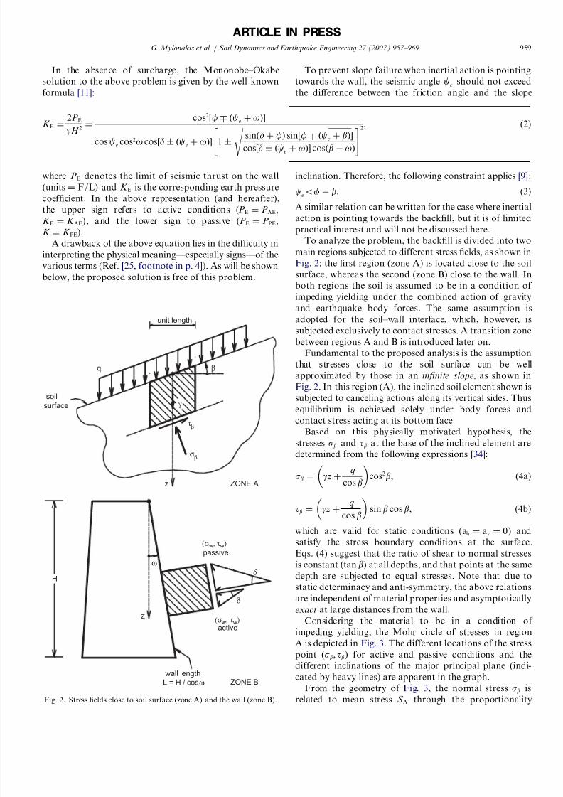
To analyze the problem, the backfill is divided into two

main regions subjected to different stress fields, as shown in

Fig. 2: the first region (zone A) is located close to the soil

surface, whereas the second (zone B) close to the wall. Inboth regions the soil is assumed to be in a condition of 

impeding yielding under the combined action of gravity

and earthquake body forces. The same assumption is

adopted for the soil–wall interface, which, however, is

subjected exclusively to contact stresses. A transition zone

between regions A and B is introduced later on.

Fundamental to the proposed analysis is the assumption

that stresses close to the soil surface can be well

approximated by those in an   infinite slope, as shown in

Fig. 2. In this region (A), the inclined soil element shown is

subjected to canceling actions along its vertical sides. Thus

equilibrium is achieved solely under body forces and

contact stress acting at its bottom face.Based on this physically motivated hypothesis, the

stresses  sb   and   tb  at the base of the inclined element are

determined from the following expressions  [34]:

sb ¼   gz þ   q

cosb

cos2b, (4a)

tb ¼   gz þ   q

cos b

sinb cos b, (4b)

which are valid for static conditions (ah ¼ av ¼ 0) and

satisfy the stress boundary conditions at the surface.

Eqs. (4) suggest that the ratio of shear to normal stresses

is constant ðtan bÞ at all depths, and that points at the same

depth are subjected to equal stresses. Note that due to

static determinacy and anti-symmetry, the above relations

are independent of material properties and asymptotically

exact  at large distances from the wall.

Considering the material to be in a condition of 

impeding yielding, the Mohr circle of stresses in region

A is depicted in Fig. 3. The different locations of the stress

point (sb; tb) for active and passive conditions and the

different inclinations of the major principal plane (indi-

cated by heavy lines) are apparent in the graph.

From the geometry of   Fig. 3, the normal stress   sb   is

related to mean stress   S A   through the proportionality

ARTICLE IN PRESS

soil

surface

z ZONE A

ZONE B

τβ

σβ

γ 

unit length

q β

H

z

active

 wall length

L = H / cosω 

δ

δ

(σw, τw)

(σw, τw)

ω 

passive

Fig. 2. Stress fields close to soil surface (zone A) and the wall (zone B).

K E ¼ 2P E

gH 2 ¼   cos2½f ðce þoÞ

cosce cos2o cos½d ðce þ oÞ   1  ffiffiffiffiffiffiffiffiffiffiffiffiffiffiffiffiffiffiffiffiffiffiffiffiffiffiffiffiffiffiffiffiffiffiffiffiffiffiffiffiffiffiffiffiffiffiffiffiffiffiffiffiffiffiffiffiffiffisinðdþ fÞ sin½f ðce þ bÞ

cos½d ðce þ oÞ cosðboÞs " #2

, (2)

G. Mylonakis et al. / Soil Dynamics and Earthquake Engineering 27 (2007) 957–969   959

7/17/2019 14102015MononobeOkabeMylonakis Et Al SDEE 2007

http://slidepdf.com/reader/full/14102015mononobeokabemylonakis-et-al-sdee-2007 5/14

relation

sb ¼ S A½1 sinf cosðD1 bÞ, (5)

where  D1  denotes the Caquot angle  [23,28] given by

sinD1 ¼  sinb

sinf. (6)

For points in region B, it is assumed that stresses are

functions exclusively of the vertical coordinate and obey

the strength criterion of the frictional soil–wall interface, as

shown in Fig. 2. Accordingly, at orientations inclined at an

angle  o   from vertical,

tw ¼ sw tan d, (7)

where   sw   and   tw   are the normal and shear tractions

on the wall, at depth   z. The above equation is asympto-

tically   exact   for points in the vicinity of the wall. The

corresponding Mohr circle of stresses is depicted in  Fig. 3.

The different signs of shear tractions for active and passive

conditions follow the directions shown in   Fig. 2   (passive

wall tractions pointing upward, active tractions pointing

downward), which comply with the kinematics of the

problem. This is in contrast with the widespread view that

solutions based on equilibrium totally ignore the displace-

ment field [29].

From the geometry of   Fig. 3, normal traction   sw   is

related to mean stress  S B   through the expression

sw ¼ S B½1 sinf cosðD2 dÞ, (8)

where  D2  is the corresponding Caquot angle given by

sinD2 ¼   sin d

sinf. (9)

In light of the foregoing, it becomes evident that the

orientation of stress characteristics in the two regions is

different and varies for active and passive conditions. In

addition, the mean stresses   S A   and   S B   generally do not

coincide, which suggests that a Rankine-type solution

based on a single stress field is not possible.

To determine the separation of mean stresses  S A  and S Band ensure a smooth transition in the orientation of 

principal planes in the two zones, a logarithmic  stress fan2

is adopted in this study, centered at the top of the wall. In

the interior of the fan, principal stresses are gradually

rotated by the angle y separating the major principal planes

in the two regions, as shown in   Fig. 4. This additional

condition is written as  [10]

S B ¼ S A expð2y tanfÞ. (10)

The negative sign in the above equation pertains to the case

where S BoS A  (e.g., active case) and vice versa. The above

equation is an exact solution of the governing Ko ¨ tter

equations for a weightless frictional material. For a

material with weight, the solution is only approximate as

Kotter’s equations are not perfectly satisfied   [25–27]. Inother words, the log spiral fan accurately transmits stresses

applied at its boundaries, but handles only approximately

body forces imposed within its volume. The error is

expected to be small for active conditions (which are of 

key importance in design), because of the small opening

angle of the fan, and bigger for passive conditions. As a

result, the above solution cannot be interpreted in the

context of limit analysis theorems. Nevertheless, it will be

shown that these violations are of minor importance from a

practical viewpoint.

 2.1. Solution without earthquake loading

The total thrust on the wall due to surcharge and gravity

loading is obtained by the well-known expression [10]

P ¼ K qqH þ 1

2K ggH 2, (11)

which is reminiscent (though not equivalent) of the bearing

capacity equation of a strip surface footing on cohesionless

soil. In the above equation,   K q   and   K g   denote the earth

pressure coefficients due to surcharge and self-weight,

respectively.

ARTICLE IN PRESS

passive

∆1φ

β

∆1−β S A

∆1+β

∆1

σ1A

active

 s o i l  s u

 r f a c e 

activecase

passivecase

 

∆2+δφ

SB∆2−δδ

δ

∆2

σ1B

passive

active

 wallplane

active

wall

plane

passive

(σβ,τβ)

(σw, τw)

(σw,τw)

(σβ,τβ)

ZONE A

ZONE B

Fig. 3. Mohr circles of effective stresses and inclination of the major

principal planes in zones A and B.

2This should not be confused with log-spiral shaped failure surfaces

used in kinematic solutions of related problems.

G. Mylonakis et al. / Soil Dynamics and Earthquake Engineering 27 (2007) 957–969960

7/17/2019 14102015MononobeOkabeMylonakis Et Al SDEE 2007

http://slidepdf.com/reader/full/14102015mononobeokabemylonakis-et-al-sdee-2007 6/14

Combining Eqs. (5), (8) and (10), and integrating over

the height of the wall, it is straightforward to show that the

earth pressure coefficient  K g   is given by [39]

K g ¼cos

ðo

b

Þcos b

cos d cos2 o

1

sinf cos

ðD2

d

Þ1 sinf cosðD1 bÞ expð2y tanfÞ,   ð12Þ

where

2y ¼ D2 ðD1 þ dÞ þ b 2o   (13)

is twice the angle separating the major principal planes in

zones A and B (Fig. 4). The convention regarding double

signs in the above equations is as before.

It is also straightforward to show that the surcharge

coefficient K q is related to K g through the simple expression

K q ¼

K gcoso

cosðo bÞ, (14)

which coincides with the kinematic solution of Chen and

Liu   [31], established using a Coulomb mechanism. Note

that for a horizontal backfill (b ¼ 0), coefficients K q  and  K gcoincide regardless of wall inclination and material proper-

ties. Eq. (14) represents an  exact  solution for a weightless

material with surcharge. A simplified version of the above

solutions, restricted to the special case of a vertical wallwith horizontal backfill and no surcharge (o ¼ b ¼ 0;

q ¼ 0), has been derived by Lancelotta   [30]. Another

simplified solution, which, however, contains some alge-

braic mistakes (see application example in the Appendix)

and is restricted to active conditions and no surcharge, has

been presented by Powrie [35].

 2.2. Solution including earthquake loading

Recognizing that earthquake action imposes a resultant

thrust in the backfill inclined by a   constant  angle  ce   from

vertical (Fig. 1), it becomes apparent that the pseudo-dynamic problem does not differ fundamentally from the

corresponding static problem, as the former can be obtained

from the latter through a rotation of the reference axes by

the seismic angle  ce, as shown in   Fig. 5. In other words,

considering  ce  does not add an extra physical parameter to

the problem, but simply alters the values of the other

variables. This property of   similarity   was apparently first

employed by Briske   [32]   and later by Arango   [8,9]   in the

analysis of related problems. Application of the concept to

the present analysis yields the following algebraic transfor-

mations, according to the notation of  Fig. 5:

b ¼ bþ ce, (15)

o ¼ oþ ce, (16)

ARTICLE IN PRESS

H

ψ eω 

ψ e

ψ e

H*

ω *

β

β*

Fig. 5. Similarity transformation for analyzing the pseudo-dynamic

seismic problem as a gravitational problem. Note the modified wall

height   ðH Þ, backfill slope   ðbÞ, and wall inclination   ðoÞ   in the

transformed geometry. Also note that the rotation should be performed

in the opposite sense (i.e., clockwise) for passive pressures ðceo0Þ.

ω 

z

zone B

2 2

π ∆2−δ−

zone Aθ AB

∆1 + ββ 2

 ACTIVE CONDITIONS

ω 

θ AB

z

zone A

PASSIVE CONDITIONS

∆2 + δ

2

2 2

π −

β

zone B

∆1−β

Fig. 4. Rotation of major principal planes between zones A and B for

active and passive conditions.

G. Mylonakis et al. / Soil Dynamics and Earthquake Engineering 27 (2007) 957–969   961

7/17/2019 14102015MononobeOkabeMylonakis Et Al SDEE 2007

http://slidepdf.com/reader/full/14102015mononobeokabemylonakis-et-al-sdee-2007 7/14

H  ¼ H  cosðoþ ceÞ= coso, (17)

g ¼ gð1 avÞ= cosce, (18)

q ¼ qð1 avÞ= cosce. (19)

The modification in g  and q  is due to the change in length of 

the corresponding vectors (Fig. 1) as a result of inertialaction. To obtain Eq. (19), it has been tacitly assumed that

the surcharge responds to the earthquake motion in the

same manner as the backfill and, thereby, the transformed

surcharge remains vertical. Note that this is not an essential

hypothesis—just a convenient (reasonable) assumption from

an analysis viewpoint. Understandably, the strength para-

meters  f  and  d  are invariant to the transformation.

In the light of the above developments, the soil thrust

including earthquake action can be determined from the

modified expression:

P E ¼ K qqH  þ 1

2K gg

H 2, (20a)

in which parameters  b,  o,  H ,  g, and  q  have been replaced

by their transformed counterparts. The symbols  K q  and  K gdenote the surcharge and self-weight coefficients in the

modified geometry, respectively.

Substituting Eqs. (15) through (19) in Eq. (20a) yields the

modified earth pressure expressions

P E ¼ ð1 avÞ½K EqqH þ 1=2 K E ggH 2, (20b)

where

K Eg ¼ cosðo bÞ cosðbþ ceÞcosce cos d cos2 o

  1 sinf cosðD2 dÞ1 sinf cos½D1 ðbþ ceÞ

expð2yE tanfÞ,

ð21Þ

which encompasses seismic action and can be used in the

context of Eq. (11). In the above equation,

2yE ¼ D2 ðD1þ dÞ þ b 2o ce   (22)

is twice the revolution angle of principal stresses in

the two regions under seismic conditions;   D1   equalsArcsin½sinðbþ ceÞ= sinf, following Eqs. (6) and (15).

The seismic earth pressure coefficient K Eq  is obtained as

K Eq ¼ K Egcoso

cosðo bÞ, (23)

which coincides with the static solution in Eq. (14).

The horizontal component of soil thrust is determined

from the   actual    geometry, as in the gravitational

problem

P EH 

 ¼P E cos

ðo

d

Þ. (24)

 2.3. Seismic component of soil thrust

Following Seed and Whitman [8], the seismic component

of soil thrust is defined from the difference:

DP E ¼ P E P , (25)

which is mathematically valid, as the associated vectors P Eand   P   are coaxial. Nevertheless, the physical meaning of 

DP E   is limited given that the stress fields (and the

corresponding failure mechanisms) in the gravitational

and seismic problems are different. In addition,   DP Ecannot be interpreted in the context of limit analysistheorems, as the difference of  P E  and P  is neither an upper

nor a lower bound to the true value.

ARTICLE IN PRESS

Table 1

Comparison of results for active and passive earth pressures predicted by various methods

o   0   20   20

f   20   30   40   30   30

d   0   10   0   15   0   20   0   15   0   15

(a)  K Ag —valuesa

Coulomb 0.490 0.447 0.333 0.301 0.217 0.199 0.498 0.476 0.212 0.180Kinematic limit analysis  [31]   0.490 0.448 0.333 0.303 0.217 0.200 0.498 0.476 0.218 0.189

Zero extension [33]   0.49 0.41 0.33 0.27 0.22 0.17 — — — —  

Slip line [28]   0.490 0.450 0.330 0.300 0.220 0.200 0.521 0.487 0.229 0.206

Proposed stress limit analysis 0.490 0.451 0.333 0.305 0.217 0.201 0.531 0.485 0.237 0.217

(b)  K Pg —valuesb

Coulomb 2.04 2.64 3.00 4.98 4.60 11.77 2.27 3.162 5.34 12.91

Kinematic limit analysis  [31]   2.04 2.58 3.00 4.70 4.60 10.07 2.27 3.160 5.09 8.92

Zero extension [33]   2.04 2.55 3.00 4.65 4.60 9.95 — — — —  

Slip line [28]   2.04 2.55 3.00 4.62 4.60 9.69 2.16 3.16 5.06 8.45

Proposed stress limit analysis 2.04 2.52 3.00 4.44 4.60 8.92 2.13 3.157 4.78 7.07

The results for   d ¼ o ¼ 0 are identical for all methods. Note the decrease in   K Pg   values as we move from top to bottom in each column, and the

corresponding increase in  K Ag;  b ¼ 0   (modified from Chen and Liu [31]).aK Ag

 ¼P A=1

2gH 2.

bK Pg ¼ P P=12 gH 2.

G. Mylonakis et al. / Soil Dynamics and Earthquake Engineering 27 (2007) 957–969962

7/17/2019 14102015MononobeOkabeMylonakis Et Al SDEE 2007

http://slidepdf.com/reader/full/14102015mononobeokabemylonakis-et-al-sdee-2007 8/14

3. Model verification and results

Presented in   Table 1   are numerical results for gravita-

tional active and passive pressures  ðK Ag; K PgÞ   from the

present solution and established solutions from the

literature. The predictions are in good agreement (largest

discrepancy about 10%), with the exception of Coulomb’smethod which significantly overestimates passive pressures.

Moving from the top to the bottom of each column, an

increase in K Ag  values and a decrease in  K Pg  values can be

observed. This is easily understood given the non-

conservative nature of the first two solutions (Coulomb,

Chen), and the conservative nature of the last two

(Sokolovskii   [28], proposed). This observation does not

hold for the ‘‘zero extension line’’ solution of Habibagahi

and Ghahramani   [33], which cannot be classified in the

context of limit analysis theorems.

Results for gravitational active pressures on a rough

inclined wall obtained according to three different methods

as a function of the slope angle  b, are shown in Fig. 6. The

performance of the proposed solution is good (maximum

deviation from Chen’s solution about 10%—despite the

high friction angle of 45) and elucidates the accuracy of 

the predictions. The performance of the simplified solution

of Caquot and Kerisel [23] versus that of Chen and Liu [31]

is as expected.

Corresponding predictions for passive pressures are

given in   Fig. 7, for a wall with negative backfill slope

inclination, as a function of the wall roughness   d. The

agreement of the various solutions, given the sensitivity of passive pressure analyses, is very satisfactory. Of particular

interest are the predictions of Sokolovskii’s   [28]   and

Lee and Herington’s   [36]   methods, which, surprisingly,

exceed those of Chen for rough walls. This trend is

particularly pronounced for horizontal backfill and values

of   d  above approximately 10  and has been discussed by

Chen and Liu [31].

Results for active seismic earth pressures are given in

Fig. 8, referring to cases examined in the seminal study of 

Seed and Whitman [8], for a reference friction angle of 35.

Naturally, active pressures increase with increasing levels

of seismic acceleration and slope inclination and decrease

with increasing friction angle and wall roughness. The

conservative nature of the proposed analysis versus the

Mononobe–Okabe (M–O) solution is evident in the graphs.

The trend is more pronounced for high levels of horizontal

seismic coefficient ðah40:25Þ, smooth walls, level backfills,

and high friction angles. Conversely, the trend becomes

weaker with steep backfills, rough walls, and low friction

angles.

A similar set of results is shown in Fig. 9, for a reference

friction angle of 40. The following interesting observations

can be made: First: the predictions of the proposed analysis

are in good agreement with the results from the kinematic

analysis of Chen and Liu [31], over a wide range of material

ARTICLE IN PRESS

H

ω 

β

P A

Slope Angle of Backfill, °

0 5 10 15 20 25

   C  o  e   f   f   i  c   i  e  n   t  o

   f   A  c   t   i  v  e   E  a  r   t   h   P  r  e  s  s  u  r  e ,

   K   A  γ

0.0

0.1

0.2

0.3

0.4

0.5

0.6

Chen & Liu(1990)

Caquot & Kerisel (1948)

Proposed Stress Limit Analysis

ω = 0°

ω = −20°

ω = 20°

 

1K A=P A/ (2 H

2

)

= 45°,  = 2/ 3

δ

Fig. 6. Comparison of results for active earth pressures predicted by

different methods (modified from Chen [10]).

 Angle of Wall Friction, °

0 10 20 30

   C  o  e   f   f   i  c   i  e  n   t  o   f   P  a  s  s   i  v  e   E  a  r   t   h   P  r  e  s  s  u  r  e ,   K

   P  γ

0

1

2

3

4

5

Lee & Herington (1972)

Chen & Liu (1990)

Sokolovskii (1965)

Proposed Stress Limit Analysis

PP H

δω 

KP=PP

1/( H2 )

2

 = 0°

 = −10°

=−20°

β

 = 30°,  = 20°

Fig. 7. Comparison of results for passive earth pressures by predicted by

different methods (modified from Chen and Liu [31]).

G. Mylonakis et al. / Soil Dynamics and Earthquake Engineering 27 (2007) 957–969   963

7/17/2019 14102015MononobeOkabeMylonakis Et Al SDEE 2007

http://slidepdf.com/reader/full/14102015mononobeokabemylonakis-et-al-sdee-2007 9/14

and geometric parameters.  Second , the present analysis is

conservative in all cases.  Third , close to the slope stability

limit (Fig. 9d), or for high accelerations and large wall

inclinations (Fig. 9c), Chen’s predictions are less accurate

than those of the elementary M–O solution. In the same

extreme conditions, the proposed solution becomes ex-

ceedingly conservative, exceeding M–O predictions by

about 35%. Note that whereas the M–O and the proposed

solution break down in the slope stability limit, Chen’s

solution allows for spurious mathematical predictions of 

active thrust beyond the limit, as evident in Fig. 9d. Fourth,

with the exception of the aforementioned extreme cases,

Chen’s and M–O predictions remain close over the whole

range of parameters examined. The improvement in the

predictions of the former over the latter is marginal.

Results for seismic passive pressures (resistances) are

shown in Fig. 10 for the common case of a rough vertical

wall with horizontal backfill. Comparisons of the proposed

solution with results from the M–O and Chen’s kinematic

methods are provided on the left graph (Fig. 10a). The

predictions of the stress solutions are, understandably,

lower than those of Chen and Liu, whereas M–O

predictions are very high (i.e., unconservative)—especially

for friction angles above 37. Given the sensitivity of 

passive pressure analyses, the performance of the proposed

method is deemed satisfactory.

An interesting comparison is presented in   Fig. 10b:

average predictions from the two closed-form solutions

(M–O solution and proposed stress solution) are plotted

against the rigorous numerical results of Chen and

Liu  [31]. Evidently, in the range of most practical interest

ð30ofo40Þ, the discrepancies in the results have been

drastically reduced. This suggests that the limit equilibrium

(kinematic) M–O solution and the proposed static solution

overestimate and underestimate, respectively, passive

resistances by the same amount in the specific range of 

ARTICLE IN PRESS

Horizontal Seismic Coefficient, ah

0.0 0.1 0.2 0.3 0.4 0.5   C  o  e   f   f   i  c   i  e  n   t  o   f   S  e   i  s  m   i  c   A  c   t   i  v  e

   E  a  r   t   h   P  r  e  s  s  u  r  e ,

   K   Α   E

0.0

0.1

0.2

0.3

0.4

0.5

0.6

0.7

M - O Analysis

Proposed Stress Limit Analysis

0.0 0.1 0.2 0.3 0.4 0.5

   K   Α   E  γ  c  o  s   δ

0.0

0.1

0.2

0.3

0.4

0.5

0.6

0.7

M - O Analysis

Proposed Stress Limit Analysis

Horizontal Seismic Coefficient, ah

0.0 0.1 0.2 0.3 0.4 0.5

   K   Α   E  γ

  c  o  s   δ

0.0

0.1

0.2

0.3

0.4

0.5

0.6

0.7

Horizontal Seismic Coefficient, ah

35°

40°

0.0 0.1 0.2 0.3 0.4 0.5

   K   Α   E  γ

  c  o  s   δ

0.0

0.1

0.2

0.3

0.4

0.5

0.6

0.7

M- O Analysis

Proposed Stress Limit Analysis

Horizontal Seismic Coefficient, ah

M- O Analysis

Proposed Stress Limit Analysis

H  

P AE

γ ah

1K AEγ =P

 AE/( H2)

2

H

P AE

δ γ ah

1K AEγ =P AE/ ( H2)

2

H

P AE

δ γ ah

1K AEγ =P AE/( H2)

2

HP AE

  γ ah

1K AEγ =P AE/ ( H2)2

 = 0°

 = 20°

= 35° ; = / 2= 30°

=  = 0°

=/ 2 

=  = 0°

=/ 2 

= 0°

= 35°

= = 0° = = 0°

=/ 2 

= 0°

= 35°

γ 

γ  γ 

β

γ 

δ

Fig. 8. Comparison of active seismic earth pressures predicted by the proposed solution and from conventional M–O analysis, for different geometries,

material properties and acceleration levels; av ¼ 0 (modified from Seed and Whitman [8]).

G. Mylonakis et al. / Soil Dynamics and Earthquake Engineering 27 (2007) 957–969964

7/17/2019 14102015MononobeOkabeMylonakis Et Al SDEE 2007

http://slidepdf.com/reader/full/14102015mononobeokabemylonakis-et-al-sdee-2007 10/14

properties. Accordingly, this averaging might be warranted

for design applications involving passive pressures.

Results for the earth pressure coefficient due to

surcharge K qE  (Eq. (23)) are presented in  Fig. 11, for both

active and passive conditions involving seismic action. The

agreement between the stress solution and the numerical

results of Chen and Liu [31] is excellent in the whole range

of parameters examined (except perhaps for active

pressures, where ah ¼ 0:3). As expected, M–O solution

performs well for active pressures, but severely over-

estimates the passive.

3.1. Distribution of earth pressures on the wall: analytical 

 findings

Mention has already been made that in the realm

of pseudo-dynamic analysis, there is no fundamental

physical difference between gravitational and seismic earth

pressures. Eqs. (4) indicate that stresses in the soil vary

linearly with depth (stress fan does not alter this

dependence), which implies that both gravitational and

seismic earth pressures vary linearly along the back of wall.

In the absence of surcharge, the distribution becomes

ARTICLE IN PRESS

M - O Analysis

Kinematic Limit Analysis (Chen & Liu 1990)

Proposed Stress Limit Analysis

M - O Analysis

Kinematic Limit Analysis (Chen & Liu 1990)

Proposed Stress Limit Analysis

M - O Analysis

Kinematic Limit Analysis (Chen & Liu 1990)

Proposed Stress Limit Analysis

M - O Analysis

Kinematic Limit Analysis(Chen & Liu 1990)

Proposed Stress Limit Analysis

H δ

ω 

γ γ ah

P AE

Hγ 

δH γ δ

0.0 0.1 0.2 0.3 0.4

   K   A   E  γ  c  o  s   δ

0.1

0.2

0.3

0.4

0.5

0.6

Horizontal Seismic Coefficient, ah

0.0 0.1 0.2 0.3 0.4

   C  o  e   f   f   i  c   i  e  n   t  o   f   S  e   i  s  m   i  c   A

  c   t   i  v  e   E  a  r   t   h   P  r  e  s  s  u  r  e ,

   K   A   E  γ

0.0

0.2

0.4

0.6

0.8

1.0

1.2

1.4

1.6

φ / 3

0°

slope

stability

limit

-20 -10 0 10 20

   C  o  e   f   f   i  c   i  e  n   t  o   f   S  e   i  s  m   i  c   A

  c   t   i  v  e   E  a  r   t   h   P  r  e  s  s  u  r  e ,

   K   A   E  γ

0.0

0.2

0.4

0.6

0.8

1.0

15°

ω  = 0°

15°

25 30 35 40 45

   C  o  e   f   f   i  c   i  e  n   t  o   f   S  e   i  s  m   i  c   A  c   t   i  v  e   E  a  r   t   h

   P  r  e  s  s  u  r  e ,

   K   A   E  γ

0.1

0.2

0.3

0.4

0.5

0.6

0.7

0.10

ah = 0

0.20

0.30

H δ

β

γ P AE

P AEP AE

γ ah

γ ahγ ah

 1

K AEγ = P AE/ ( γ H2)2   γ H2)

1K AEγ =P AE/ (

2

  γ H2)1

K AEγ =P AE/ (2

 γ H2)1

K AEγ =P

 AE/ (

2

Friction Angle, °

Slope Angle of Backfill, ° Horizontal Seismic Coefficient, ah

= 40°;ah = 0.20 ;  = / 2 = 40°; = 0° ;  = / 2

   =  0

  δ  =  / 

 2   =

 

 = = 0° ; = 40° = = 0° ; = 2/3

 β = φ  / 2

Fig. 9. Comparison of active seismic earth pressures predicted by different methods, for different geometries, material properties, and acceleration levels;

f¼

40, av

 ¼0 (modified from Chen and Liu  [31]).

G. Mylonakis et al. / Soil Dynamics and Earthquake Engineering 27 (2007) 957–969   965

7/17/2019 14102015MononobeOkabeMylonakis Et Al SDEE 2007

http://slidepdf.com/reader/full/14102015mononobeokabemylonakis-et-al-sdee-2007 11/14

proportional with depth, as in the Rankine solution.

Accordingly, the point of application of seismic thrust is

located at a height of  H =3 above the base of the wall. It is

well known from experimental observations and rigorous

numerical solutions, that this is not generally true. The

source of the difference lies in the distribution of inertial

forces in the soil mass (which is often sinusoidal like— 

following the time-varying natural mode shapes of the

deposit), as well as the various kinematic boundary

conditions (wall flexibility, foundation compliance, pre-

sence of supports). Studying the above factors lies beyond

the scope of this article, and like will be the subject of a

future publication. Some recent developments are provided

in the Master thesis of the second author  [39] as well as in

Refs. [11,16–18,37,38].

4. Discussion: simplicity and symmetry

It is instructive to show that the proposed solution can

be derived essentially by inspection, without tedious

algebraic manipulations as in the classical equations.

Indeed, basis of Eq. (12) is the familiar Rankine ratio

ð1 sinfÞ=ð1 sinfÞ. The terms cosðD2 dÞ and cosðD1 bÞ   in the numerator and denominator of the expression

reflect the fact that stresses   sb   and   sw   are not principal.

Both terms involve the same double signs as their multi-

pliers ( sinf   and   sinf, respectively). Angle   b   and

associated angle  D1  have to be in the denominator, as an

increase in their value must lead to an increase in active

thrust. The exponential term is easy to remember and

involves the same double signðÞ  as the other terms in the

ARTICLE IN PRESS

H

γ 

PPEγ ah γ ahδ

25 30 35 40 45   C  o  e   f   f   i  c   i  e  n   t  o   f   S  e   i  s  m   i  c   P  a  s  s   i  v  e   E  a  r   t   h   P  r  e  s  s  u  r  e ,

   K   P   E  γ

0

5

10

15

20

25

Kinematic Limit Analysis (Chen & Liu1990)

Proposed Stress Limit Analysis

Kinematic Limit Analysis (Chen & Liu1990)

 Average of M-O & Proposed Stress Limit Analysis

ah = 0

Mononobe -Okabe(a

h=0)

25 30 35 40 450

5

10

15

20

25

 -0.1

 -0.2

 -0.3 ah = 0

-0.1

-0.2

-0.3

H

γ 

PPE δ

 1

KPE

=PPE/ ( H

2)2

 1

KPE

=PPE/ ( H

2)2

 Angle of Internal Friction, °  Angle of Internal Friction, °

 = 2 / 3

= 0°, = 0°

a b

Fig. 10. Comparison of results for passive seismic resistance on a rough wall predicted by various methods (modified from Chen and Liu [31]).

H

P

δ

a q

PH

δ

q

a q

Kinematic Limit Analysis (Chen & Liu 1990)

Proposed Stress Limit Analysis

Friction Angle, φ o

25 30 35 40 450

5

10

15

20

    K

   P   E  q

  =

   P   P   E    /

  q   H

Mononobe - Okabe(ah = 0)

0.1

ah = 0

0.2

0.3

Friction Angle, φ o

25 30 35 40 450.1

0.2

0.3

0.4

0.5

0.6

0.7

Kinematic Limit Analysis (Chen & Liu 1990)

Proposed Stress Limit Analysis

   K   A   E  q

  =

   P   A   E    /

  q   H

 β ω ==  0o

δ = 2 / 3 φ

0.1

ah = 0

0.2

0.3

ω = β =  0o

δ = 2 / 3 φ

Fig. 11. Variation of  K AEq   and K PEq   values with f —angle for different acceleration levels.

G. Mylonakis et al. / Soil Dynamics and Earthquake Engineering 27 (2007) 957–969966

7/17/2019 14102015MononobeOkabeMylonakis Et Al SDEE 2007

http://slidepdf.com/reader/full/14102015mononobeokabemylonakis-et-al-sdee-2007 12/14

numerator. With reference to the factors outside the

brackets, 1= cos dð¼ ffiffiffiffiffiffiffiffiffiffiffiffiffiffiffiffiffiffiffi

1 þ tan2dp 

  Þ   stands for the vectorial

sum of shear and normal tractions at the wall–soil

interface. Factor cos b   arises from the equilibrium of the

infinite slope in Eq. (4a). Finally, cosðo bÞ=cos2o   is a

geometric factor arising from the integration of stresses

along the back of the wall, and is associated with theinclination of the wall and backfill.

In light of the above, the solution for gravitational

pressures can be expressed by the single equation

K g ¼ cosðo bÞ cos b

cos d cos2o

  1 sinf cosðD2 dÞ1 þ sinf cos½D1 þ b

expð2y tanfÞ,   ð26Þ

which is valid for both active conditions (using positive

values for f  and dÞ   and passive conditions (using negative

values for  f  and  dÞ. It is straightforward to show that this

property is not valid for the Mononobe–Okabe solutions in

Eq. (4). The lack of symmetry in the limit equilibrium

solutions can be attributed to the maximization and

minimization operations involved in deriving the limit

thrusts. An application example elucidating the simplicity

of the solution is provided below.

5. Conclusions

A stress plasticity solution was presented for determining

gravitational and earthquake-induced earth pressures on

gravity walls retaining cohesionless soil. The proposed

solution incorporates idealized, yet realistic wall geometries

and material properties. The following are the mainconclusions of the study:

(1) The proposed solution is simpler than the classical

Coulomb and Mononobe–Okabe equations. The main

features of the mathematical expressions, including

signs, can be deduced by physical reasoning, which is

hardly the case with the classical equations. Also, the

proposed solution is   symmetric   with respect to active

and passive conditions, as it can be expressed by a

single equation with opposite signs for soil friction

angle and wall roughness.

(2) Extensive comparisons with established numerical

solutions indicate that the proposed solution is   safe,

as it overestimates active pressures and under-predicts

the passive. This makes the method appealing for use in

practical applications.

(3) For active pressures, the accuracy of the solution is

excellent (maximum observed deviation from numerical

data is about 10%). The largest deviations occur for

high seismic accelerations, high friction angles, steep

backfills, and negative wall inclinations.

(4) For passive resistances, the predictions are also

satisfactory. However, the error is larger—especially

at high friction angles. Nevertheless, the improvement

over the M–O predictions is dramatic. Taking the

average between the predictions of the M–O solution

and the proposed stress solution (both available in

closed forms) yields results which are comparable to

those obtained from rigorous numerical solutions.

(5) The pseudo-dynamic seismic problem can be deduced

from the corresponding static problem through a

revolution of the reference axes by the seismic anglece   (Fig. 5). This similarity suggests that the Coulomb

and M–O solutions are essentially equivalent.

(6) Contrary to the overall gravitational-seismic thrust  P E,

the purely seismic component  DP E ¼ P E P  cannot be

put in the context of a lower or an upper bound. This

holds even when  P E  and P  are rigorous upper or lower

bounds.

(7) In the realm of the proposed model, the distribution of 

earth pressures on the back of the wall is linear with

depth for both gravitational and seismic conditions.

This is not coincidental given the similarity between the

gravitational and pseudo-dynamic problem.

It should be emphasized that the verification of the

proposed solution was restricted to analytical—not experi-

mental results. Detailed comparisons against experimental

results, including distribution of earth pressures along the

wall, will be the subject of a future publication.

Acknowledgments

The authors are indebted to Professor Dimitrios

Atmatzidis for his constructive criticism of the work.

Thanks are also due to two anonymous reviewers whose

comments significantly improved the original manuscript.

Appendix A. Application example

Active and passive earth pressures will be computed for a

gravity wall of height   H  ¼ 5 m, inclination   o ¼ 5   and

roughness   d ¼ 20, retaining an inclined cohesionless

material with   f ¼ 30,   g ¼ 18kN=m3 and   b ¼ 15, sub-

 jected to earthquake accelerations ah ¼ 0:2 and av ¼ 0. The

static counterpart of the problem has been discussed by

Powrie [35].

The inclination of the resultant body force in the backfill

is obtained from Eq. (1):

ce ¼ arctanð0:2Þ ¼ 11:3. (A.1)

The two Caquot angles are determined from Eqs. (6), (9)

and (15) as

D1 ¼ sin

1½sinð15 þ 11:3Þ= sin 30 ¼ 62:4, (A.2)

D2 ¼ sin1½sinð20Þ= sin 30 ¼ 43:2

. (A.3)

The angle separating the major principal planes in regions

A and B is computed from Eq. (21):

2yE ¼ 43:2 ð62:4 þ 20Þ þ 15 2 5 11:3 ¼ 45:5.

(A.4)

ARTICLE IN PRESS

G. Mylonakis et al. / Soil Dynamics and Earthquake Engineering 27 (2007) 957–969   967

7/17/2019 14102015MononobeOkabeMylonakis Et Al SDEE 2007

http://slidepdf.com/reader/full/14102015mononobeokabemylonakis-et-al-sdee-2007 13/14

Based on the above values, the earth pressure coefficient is

obtained from Eq. (21):

K AEg ¼ cosð5 15Þ cosð15 þ 11:3Þcos 11:3cos20cos2 5

  1 sin30cosð43:2 20Þ1þ

sin 30 cos½62:4

þ ð15

þ11:3

Þ exp  þ45:5

  p

180tan30

¼ 0:82   ðA:5Þ

from which the overall active thrust on the wall is easily

determined (Eq. (11)):

P AE ¼ 1

20:82 18 52 ¼ 185 kN=m. (A.6)

Both M–O and Chen–Liu solutions yield   K AEg ¼ 0:77,

which elucidates the more conservative nature of the

proposed approach.

For the gravitational problem, the corresponding

parameters are   D1 ¼ sin1½sin15= sin30 ¼ 31:2,   D2 ¼

sin1

½sin

ð20Þ= sin 30

¼43:2

,

2y ¼ 43:2 ð31:2 þ 20Þ þ 15 2 5 ¼ 3,  K Ag ¼ 0:42.

Thus,

P A ¼ 1

2 0:42 18 52 ¼ 94:5 kN=m. (A.7)

The horizontal component of gravitational soil thrust is

determined from Eq. (24)

P AH  ¼ 94:5 cosð5 þ 20Þ ¼ 85:6 kN=m. (A.8)

Note that according to Powrie   [35], the horizontal

component is (Eq. 9.42, p. 333)

P AH  ¼ 1

2  0:395 18 52ð1 þ tan5 tan 20Þ ¼ 91:7 kN=m,

(A.9)which is clearly in error as: (1) Ka, as determined from

Powrie’s equations, should be 0.385—not 0.395; (2) the

sign in front of product ðtanb tan dÞ   should be minus

one. (3) Powrie’s equation does not encompass factor

½cosðo bÞ= coso cosb   arising from the integration of 

stresses on the back of the wall.

For the passive case, the corresponding parameters are:

ce ¼ Arctanð0:2Þ ¼ 11:3,

D1 ¼ sin

1½sinð15 11:3Þ= sin30 ¼ 7:4,

2yE ¼ 43:2 þ ð7:4 þ 20Þ þ 15 2 5 þ 11:3 ¼ 86:9.

The passive earth pressure coefficient and resistance are

obtained from Eqs. (21) and (11):

K PEg ¼ cosð5 15Þ cosð15 11:3Þcos 11:3cos20cos2 5

  1 þ sin 30 cosð43:2 þ 20Þ1 sin 30 cos½7:41 ð15 11:3Þ

exp 2yE

p

180tan 30

¼ 6:31,   ðA:10Þ

P PE ¼ 1

2 6:31 18 52 ¼ 1420 kN=m. (A.11)

The M–O and Chen–Liu solutions predict   K PEg ¼ 10:25

and 8.01, respectively. Note that the average of the two

closed-form solutions,

  ð10:25

þ6:31

Þ=2

¼8:28, is very

close to the more rigorous result by Chen and Liu.

References

[1] Coulomb CA. Essai sur une application des regles de maximis et

minimis a quelqes problemes de stratique relatifs a l’ architecture.

Memoires de mathematique et de physique. Presentes a l’ academie

royale des sciences 1776; Paris, 7: p. 343–82.

[2] Heyman J. Coulomb’s memoir on statics; an essay in the

history of civil engineering. Cambridge: Cambridge University Press;1972.

[3] Lambe TW, Whitman RV. Soil mechanics. NY: Wiley; 1969.

[4] Clough GW, Duncan JM. Earth pressures. In: Fang HY, editor.

Foundation engineering handbook. New York: Chapman & Hall;

1990. p. 223–35.

[5] Okabe S. General theory on earth pressure and seismic stability

of retaining walls and dams. J Jpn Soc Civil Eng 1924;10(6):

1277–323.

[6] Mononobe N, Matsuo O. On the determination of earth pressure

during earthquakes. In: Proceeding of the world engineering

congress, vol. 9. Tokyo; 1929. p. 179–87.

[7] Matsuo M, Ohara S. Lateral earth pressures and stability of quay

walls during earthquakes. Proceedings, second world conference on

earthquake engineering, Tokyo, Japan; 1960.

[8] Seed HB, Whitman RV. Design of earth retaining structures fordynamic loads. In: Proceedings of specialty conference on lateral

stresses in the ground and design of earth retaining structures. Ithaca,

New York: ASCE; 1970. p. 103–47.

[9] Ebeling RM, Morrison EE, Whitman RV, Liam Finn WD. A manual

for seismic design of waterfront retaining structures. US Army Corps

of Engineers, Technical Report ITL-92-11;1992.

[10] Chen WF. Limit analysis and soil plasticity. Developments in

geotechnical engineering. Amsterdam: Elsevier; 1975.

[11] Kramer SL. Geotechnical earthquake engineering. Englewood Cliffs,

NJ: Prentice-Hall; 1996.

[12] Wood JH. Earthquake induced soil pressures on structures. Doctoral

Dissertation, EERL 73–50, Pasadena, CA: California Institute of 

Technology; 1973.

[13] Steedman RS, Zeng X. The influence of phase on the calculation of 

pseudo-static earth pressure on a retaining wall. Geotechnique1990;40:103–12.

[14] Sheriff MA, Ishibashi I, Lee CD. Earth pressures against rigid

retaining walls. J Geotech Eng 1982, ASCE; 108: GT5. p. 679–96.

[15] Finn WD, Yogendrakumar M, Otsu H, Steedman RS. Seismic

response of a cantilever retaining wall: centrifuge model test and

dynamic analysis. In: Proceedings of fourth international conference

on soil dynamics and earthquake engineering. Southampton:

Computational Mechanics Publications; 1989. p. 331–431.

[16] Veletsos AS, Younan AH. Dynamic soil pressures on rigid retaining

walls. Earthquake Eng Struct Dyn 1994;23:275–301.

[17] Theodorakopoulos DD, Chassiakos AP, Beskos DE. Dynamic

pressures on rigid cantilever walls retaining poroelastic soil media.

Part I: first method of solution. Soil Dyn Earthquake Eng

2001;21(4):315–38.

[18] Theodorakopoulos DD, Chassiakos AP, Beskos DE. Dynamicpressures on rigid cantilever walls retaining poroelastic soil media.

Part II: second method of solution. Soil Dyn Earthquake Eng

2001;21(4):339–64.

[19] Pecker A. Seismic design of shallow foundations. In: Duma A, editor.

State-of-the-Art: 10th european conference on earthquake engineer-

ing. Balkema; 1995. p. 1001–10.

[20] Richards R, Elms DG. Seismic behaviour of gravity retaining walls.

J Geotechn Eng Div 1979;105(GT4):449–64.

[21] Whitman RV, Liao S. Seismic design of gravity retaining walls. US

Army Corps of Engineers, Miscellaneous paper GL-85-1; 1985.

[22] Collins IL. A note on the interpretation of Coulomb analysis of the

thrust on a rough retaining wall in terms of the limit theorems of 

plasticity theory. Geotechnique 1973;24(1):106–8.

[23] Caquot A, Kerisel L. Traite ´   de me ´ canique des sols. Paris: Gauthier-

Villars; 1948.

ARTICLE IN PRESS

G. Mylonakis et al. / Soil Dynamics and Earthquake Engineering 27 (2007) 957–969968

7/17/2019 14102015MononobeOkabeMylonakis Et Al SDEE 2007

http://slidepdf.com/reader/full/14102015mononobeokabemylonakis-et-al-sdee-2007 14/14

[24] Finn WD. Applications of limit plasticity in soil mechanics. J Soil

Mech Found Div 1967;93(SM5):101–20.

[25] Davis RO, Selvadurai APS. Plasticity and geomechanics. Cambridge:

Cambridge University Press; 2002.

[26] Atkinson J. Foundations and slopes. London: McGraw-Hill; 1981.

[27] Parry RHG. Mohr circles, stress paths and geotechnics. E&FN Spon;

1995.

[28] Sokolovskii VV. Statics of granular media. New York: PergamonPress; 1965.

[29] Papantonopoulos C, Ladanyi B. Analyse de la Stabilitee des Talus

Rocheux par une Methode Generalisee de l’Equilibre Limite. In:

Proceedings, ninth Canadian rock mechanics symposium. Montreal;

December 1973. p. 167–96 [in French].

[30] Lancelotta R. Analytical solution of passive earth pressure.

Geotechnique 2002;52(8):617–9.

[31] Chen WF, Liu XL. Limit analysis in soil mechanics. Amsterdam:

Elsevier; 1990.

[32] Briske R. Die Erdbebensicherheit von Bauwerken. Die Bautechnik

1927;5:425–30 453–7, 547–55.

[33] Habibagahi K, Ghahramani A. Zero extension theory of earth

pressure. J Geotech Eng Div 1977;105(GT7):881–96.

[34] Terzaghi K. Theoretical soil mechanics. New York: Wiley; 1943.

[35] Powrie W. Soil mechanics: concepts and applications. London:

E&FN Spon; 1997.

[36] Lee IK, Herington JR. A theoretical study of the pressures acting on

a rigid wall by a sloping earth or rock fill. Geotechnical 1972;

22(1):1–26.

[37] Ostadan F. Seismic soil pressure for building walls: an updated

approach. Soil Dyn Earthquake Eng 2005;25:785–93.

[38] Paik K, Salgado R. Estimation of active earth pressure against rigidretaining walls considering arching effects. Geotechnique 2003;

53(7):643–53.

[39] Kloukinas P. Gravitational and earthquake-induced earth pressures

on gravity walls by stress plasticity theory. Ms. Thesis, University of 

Patras; 2006 [in Greek with extended English summary].

[40] Salencon J. Applications of the theory of plasticity in soil mechanics.

New York: Wiley; 1974.

[41] Davies TG, Richards R, Chen KH. Passive pressure during seismic

loading. J Geotechn Eng 1986;112(4):479–83.

[42] Salencon J. Introduction to the yield design theory. Eur J Mech A

Solids 1990;9(5):477–500.

[43] Psarropoulos PN, Klonaris G, Gazetas G. Seismic earth pressures on

rigid and flexible retaining walls. Soil Dyn Earthquake Eng 2005;

24:795–809.

ARTICLE IN PRESS

G. Mylonakis et al. / Soil Dynamics and Earthquake Engineering 27 (2007) 957–969   969