16.1. introduction - stony brook...

16Moiré and Fringe Projection Techniques

K. Creath and J. C. Wyant

16.1. INTRODUCTION

The term “moiré” is not the name of a person; in fact, it is a French wordreferring to “an irregular wavy finish usually produced on a fabric by pressingbetween engraved rollers” (Webster's 1981). In optics it refers to a beat patternproduced between two gratings of approximately equal spacing. It can be seenin everyday things such as the overlapping of two window screens, the rescreen-ing of a half-tone picture, or with a striped shirt seen on television. The use ofmoiré for reduced sensitivity testing was introduced by Lord Rayleigh in 1874.Lord Rayleigh looked at the moiré between two identical gratings to determinetheir quality even though each individual grating could not be resolved under amicroscope.

Fringe projection entails projecting a fringe pattern or grating on an objectand viewing it from a different direction. The first use of fringe projection fordetermining surface topography was presented by Rowe and Welford in 1967.It is a convenient technique for contouring objects that are too coarse to bemeasured with standard interferometry. Fringe projection is related to opticaltriangulation using a single point of light and light sectioning where a singleline is projected onto an object and viewed in a different direction to determinethe surface contour (Case et al. 1987).

Moiré and fringe projection interferometry complement conventional holo-graphic interferometry, especially for testing optics to be used at long wave-lengths. Although two-wavelength holography (TWH) can be used to contoursurfaces at any longer-than-visible wavelength, visible interferometric environ-mental conditions are required. Moiré and fringe projection interferometry cancontour surfaces at any wavelength longer than 10-100 µm with reduced en-vironmental requirements and no intermediate photographic recording setup.

Optical Shop Testing, Second Edition, Edited by Daniel Malacara.ISBN 0-471-52232-5 © 1992, John Wiley & Sons, inc.

653

654 MOIRÉ AND FRINGE PROJECTION TECHNIQUES

Moiré is also a useful technique for aiding in the understanding of interfer-ometry.

This chapter explains what moiré is and how it relates to interferometry.Contouring techniques utilizing fringe projection, projection and shadow moiré,and two-angle holography are all described and compared. Each of these tech-niques provides the same result and can be described by a single theory. Therelationship between these techniques and holographic and conventional inter-ferometry will be shown. Errors caused by divergent geometries are described,and applications of these techniques combined with phase measurement tech-niques are presented. Further information on these techniques can be found inthe following books and book chapters: Varner (1974), Vest (1979), Hariharan(1984), Gasvik (1987), and Chiang (1978, 1983).

16.2. WHAT IS MOIRÉ?

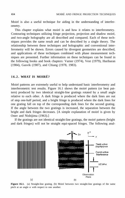
Moiré patterns are extremely useful to help understand basic interferometry andinterferometric test results. Figure 16.1 shows the moiré pattern (or beat pat-tern) produced by two identical straight-line gratings rotated by a small anglerelative to each other. A dark fringe is produced where the dark lines are outof step one-half period, and a bright fringe is produced where the dark lines forone grating fall on top of the corresponding dark lines for the second grating.If the angle between the two gratings is increased, the separation between thebright and dark fringes decreases. [A simple explanation of moiré is given byOster and Nishijima (1963).]

If the gratings are not identical straight-line gratings, the moiré pattern (brightand dark fringes) will not be straight equi-spaced fringes. The following anal-

(a) (b)

ObservationPlane

Figure 16.1. (a) Straight-line grating. (b) Moiré between two straight-line gratings of the samepitch at an angle α with respect to one another.

16.2. WHAT IS MOIRÉ? 655

ysis shows how to calculate the moire pattern for arbitrary gratings. Let theintensity transmission function for two gratings f1(x, y) and f2(x, y) be given by

(16.1)

where φ (x, y) is the function describing the basic shape of the grating lines. Forthe fundamental frequency, φ (x, y) is equal to an integer times 2 π at the centerof each bright line and is equal to an integer plus one-half times 2 π at the centerof each dark line. The b coefficients determine the profile of the grating lines(i.e., square wave, triangular, sinusoidal, etc.) For a sinusoidal line profile, is the only nonzero term.

When these two gratings are superimposed, the resulting intensity transmis-sion function is given by the product

(16.2)

The first three terms of Eq. (16.2) provide information that can be determinedby looking at the two patterns separately. The last term is the interesting one,and can be rewritten as

n and m both # 1

(16.3)

This expression shows that by superimposing the two gratings, the sum anddifference between the two gratings is obtained. The first term of Eq. (16.3)


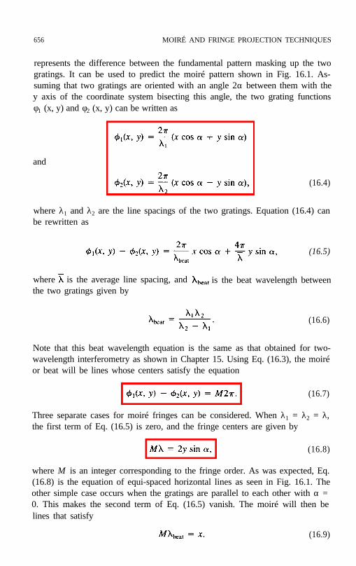
represents the difference between the fundamental pattern masking up the twogratings. It can be used to predict the moiré pattern shown in Fig. 16.1. As-suming that two gratings are oriented with an angle 2α between them with they axis of the coordinate system bisecting this angle, the two grating functionsφ1 (x, y) and φ2 (x, y) can be written as

and

(16.4)

where λ1 and λ2 are the line spacings of the two gratings. Equation (16.4) canbe rewritten as

(16.5)

where is the average line spacing, and is the beat wavelength betweenthe two gratings given by

(16.6)

Note that this beat wavelength equation is the same as that obtained for two-wavelength interferometry as shown in Chapter 15. Using Eq. (16.3), the moiréor beat will be lines whose centers satisfy the equation

(16.7)

Three separate cases for moiré fringes can be considered. When λ1 = λ2 = λ,the first term of Eq. (16.5) is zero, and the fringe centers are given by

(16.8)

where M is an integer corresponding to the fringe order. As was expected, Eq.(16.8) is the equation of equi-spaced horizontal lines as seen in Fig. 16.1. Theother simple case occurs when the gratings are parallel to each other with α =0. This makes the second term of Eq. (16.5) vanish. The moiré will then belines that satisfy

(16.9)

16.2. WHAT IS MOIRÉ 657

Same Frequency

Tilted

Different Frequencies

No Tilt Tilted

(a) (b) (c)Figure 16.2. Moiré patterns caused by two straight-line gratings with (a) the same pitch tiltedwith respect to one another, (b) different frequencies and no tilt, and (c) different frequencies tiltedwith respect to one another.

These fringes are equally spaced, vertical lines parallel to the y axis. For themore general case where the two gratings have different line spacings and theangle between the gratings is nonzero, the equation for the moiré fringes willnow be

(16.10)

This is the equation of straight lines whose spacing and orientation is dependenton the relative difference between the two grating spacings and the angle be-tween the gratings. Figure 16.2 shows moiré patterns for these three cases.

The orientation and spacing of the moiré fringes for the general case can bedetermined from the geometry shown in Fig. 16.3 (Chiang, 1983). The distanceAB can be written in terms of the two grating spacings;

(16.11)

Figure 16.3. Geometry used to determine spacingand angle of moiré fringes between two gratings ofdifferent frequencies tilted with respect to one an-other.


where θ is the angle the moiré fringes make with the y axis. After rearranging,the fringe orientation angle θ is given by

When α = 0 and and when λ1 = λ2 with α ≠ 0, θ = 90o

as expected. The fringe spacing perpendicular to the fringe lines can be foundby equating quantities for the distance DE;

(16.13)

where C is the fringe spacing or contour interval. This can be rearranged toyield

(16.14)

By substituting for the fringe orientation θ, the fringe spacing can be found interms of the grating spacings and angle between the gratings;

(16.15)

In the limit that α = 0 and λ1 ≠ λ2, the fringe spacing equals λ beat, and in thelimit that λ1 = λ2 = λ and α ≠ 0, the fringe spacing equals λ/(2 sin α). It ispossible to determine λ2 and α from the measured fringe spacing and orientationas long as λ1 is known (Chiang 1983).

16.3. MOIRÉ AND INTERFEROGRAMS

Now that we have covered the basic mathematics of moiré patterns, let us seehow moiré patterns are related to interferometry. The single grating shown inFig. 16.1 can be thought of as a “snapshot” of a plane wave traveling to theright, where the distance between the grating lines is equal to the wavelengthof light. The straight lines represent the intersection of a plane of constant phasewith the plane of the figure. Superimposing the two sets of grating lines in Fig.16.1 can be thought of as superimposing two plane waves with an angle of 2αbetween their directions of propagation. Where the two waves are in phase,bright fringes result (constructive interference), and where they are out of phase,

16.3. MOIRÉ AND INTERFEROGRAMS 659

dark fringes result (destructive interference). For a plane wave, the “grating”lines are really planes perpendicular to the plane of the figure and the dark andbright fringes are also planes perpendicular to the plane of the figure. If theplane waves are traveling to the right, these fringes would be observed by plac-ing a screen perpendicular to the plane of the figure and to the right of thegrating lines as shown in Fig. 16.1. The spacing of the interference fringes onthe screen is given by Eqn. (16.8), where λ is now the wavelength of light.Thus, the moiré of two straight-line gratings correctly predicts the centers ofthe interference fringes produced by interfering two plane waves. Since thegratings used to produce the moiré pattern are binary gratings, the moiré doesnot correctly predict the sinusoidal intensity profile of the interference fringes.(If both gratings had sinusoidal intensity profiles, the resulting moiré would stillnot have a sinusoidal intensity profile because of higher-order terms.)

More complicated gratings, such as circular gratings, can also be investi-gated. Figure 16.4b shows the superposition of two circular line gratings. Thispattern indicates the fringe positions obtained by interfering two sphericalwavefronts. The centers of the two circular line gratings can be considered thesource locations for two spherical waves. Just as for two plane waves, the spac-ing between the grating lines is equal to the wavelength of light. When the twopatterns are in phase, bright fringes are produced; and when the patterns arecompletely out of phase, dark fringes result. For a point on a given fringe, thedifference in the distances from the two source points and the fringe point is aconstant. Hence, the fringes are hyperboloids. Due to symmetry, the fringesseen on observation plane A of Fig. 16.4b must be circular. (Plane A is alongthe top of Fig. 16.4b and perpendicular to the line connecting the two sourcesas well as perpendicular to the page.) Figure 16.4c shows a binary representa-tion of these interference fringes and represents the interference pattern obtainedby interfering a nontilted plane wave and a spherical wave. (A plane wave canbe thought of as a spherical wave with an infinite radius of curvature.) Figure16.4d shows that the interference fringes in plane B are essentially straight equi-spaced fringes. (These fringes are still hyperbolas, but in the limit of largedistances, they are essentially straight lines. Plane B is along the side of Fig.16.4b and parallel to the line connecting the two sources as well as perpendic-ular to the page.)

The lines of constant phase in plane B for a single spherical wave are shownin Fig. 16.5a. (To first-order, the lines of constant phase in plane B are thesame shape as the interference fringes in plane A.) The pattern shown in Fig.16.5a is commonly called a zone plate. Figure 16.5b shows the superpositionof two linearly displaced zone plates. The resulting moiré pattern of straightequi-spaced fittings illustrates the interference fringes in plane B shown in Fig.16.4b.

Superimposing two interferograms and looking at the moiré or beat producedcan be extremely useful. The moiré formed by superimposing two different


Plane B

Figure 16.4. Interference of two spherical waves. (a) Circular line grating representing a spher-ical wavefront. (b) Moiré pattern obtained by superimposing two circular line patterns. (c) Fringesobserved in plane A. (d) Fringes observed in plane B.

16.3. MOIRÉ AND INTERFEROGRAMS

Figure 16.4. (Continued)

interferograms shows the difference in the aberrations of the two interfero-grams. For example, Fig. 16.6 shows the moiré produced by superimposingtwo computer-generated interferograms. One interferogram has 50 waves of tiltacross the radius (Fig. 16.6a), while the second interferogram has 50 waves oftilt plus 4 waves of defocus (Fig. 16.6b). If the interferograms are aligned suchthat the tilt direction is the same for both interferograms, the tilt will cancel and


(b)Figure 16.5. Moiré pattern produced by two zone plates. (a) Zone plate. (b) Straight-line friresulting from superposition of two zone plates.

only the 4 waves of defocus remain (Fig. 16.6c). In Fig. 16.6d, the two inferograms are rotated slightly with respect to each other so that the tilt willquite cancel. These results can be described mathematically by looking attwo grating functions:

nges

inter-notthe

16.3. MOIRÉ AND INTERFEROGRAMS 663

(b)

(d)

Figure 16.6. Moiré between two interferograms. (a) Interferogram having 50 waves tilt. (6) In-terferogram having 50 waves tilt plus 4 waves of defocus. (c) Superposition of (a) and (b) with notilt between patterns. (d) Slight tilt between patterns.

and

A bright fringe is obtained when

(16.16)

(16.17)

If α = 0, the tilt cancels completely and four waves of defocus remain; oth-erwise, some tilt remains in the moiré pattern.


Figure 16.7 shows similar results for interferograms containing third-orderaberrations. Spherical aberration with defocus and tilt is shown in Fig. 16.7d.One interferogram has 50 waves of tilt (Fig. 16.6a), and the other has 55 wavestilt, 6 waves third-order spherical aberration, and -3 waves defocus (Fig.16.7a). Figure 16.7e shows the moiré between an interferogram having 50waves of tilt (Fig. 16.6a) with an interferogram having 50 waves of tilt and 5waves of coma (Fig. 16.7b) with a slight rotation between the two patterns.The moiré between an interferogram having 50 waves of tilt (Fig. 16.6a) andone having 50 waves of tilt, 7 waves third-order astigmatism, and -3.5 wavesdefocus (Fig. 16.7c) is shown in Fig. 16.7f. Thus, it is possible to producesimple fringe patterns using moiré. These patterns can be photocopied ontotransparencies and used as a learning aid to understand interferograms obtainedfrom third-order aberrations.

A computer-generated interferogram having 55 waves of tilt across the ra-dius, 6 waves of spherical and -3 waves of defocus is shown in Fig. 16.7a.Figure 16.8a shows two identical interferograms superimposed with a smallrotation between them. As expected, the moiré pattern consists of nearly straightequi-spaced lines. When one of the two interferograms is slipped over, theresultant moiré is shown in Fig. 16.8b. The fringe deviation from straightnessin one interferogram is to the right and, in the other, to the left. Thus the signof the defocus and spherical aberration for the two interferograms is opposite,and the moiré pattern has twice the defocus and spherical of each of the indi-vidual interferograms. When two identical interferograms given by Fig. 16.7aare superimposed with a displacement from one another, a shearing interfero-gram is obtained. Figure 16.9 shows vertical and horizontal displacements withand without a rotation between the two interferograms. The rotations indicatethe addition of tilt to the interferograms. These types of moiré patterns are veryuseful for understanding lateral shearing interferograms.

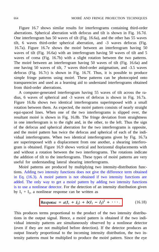
Moiré patterns are produced by multiplying two intensity-distribution func-tions. Adding two intensity functions does not give the difference term obtainedin Eq. (16.3). A moiré pattern is not obtained if two intensity functions areadded. The only way to get a moiré pattern by adding two intensity functionsis to use a nonlinear detector. For the detection of an intensity distribution givenby I1 + I2, a nonlinear response can be written as

(16.18)

This produces terms proportional to the product of the two intensity distribu-tions in the output signal. Hence, a moiré pattern is obtained if the two indi-vidual intensity patterns are simultaneously observed by a nonlinear detector(even if they are not multiplied before detection). If the detector produces anoutput linearly proportional to the incoming intensity distribution, the two in-tensity patterns must be multiplied to produce the moiré pattern. Since the eye


(b)Figure 16.8. Moire pattern by superimposing two identical interferograms (from Fig. 16.7a). (a)Both patterns having the same orientation. (b) With one pattern flipped.

is a nonlinear detector, moiré can be seen whether the patterns are added ormultiplied. A good TV camera, on the other hand, will not see moiré unlessthe patterns are multiplied.

16.4. HISTORICAL REVIEW

Since Lord Rayleigh first noticed the phenomena of moiré fringes, moiré tech-niques have been used for a number of testing applications. Righi (1887) firstnoticed that the relative displacement of two gratings could be determined byobserving the movement of the moiré fringes. The next significant advance inthe use of moiré was presented by Weller and Shepherd (1948). They usedmoiré to measure the deformation of an object under applied stress by lookingat the differences in a grating pattern before and after the applied stress. Theywere the first to use shadow moiré, where a grating is placed in front of a nonflatsurface to determine the shape of the object behind it by using the shape of themoiré fringes. A rigorous theory of moiré fringes did not exist until the mid-fifties when Ligtenberg (1955) and Guild (1956, 1960) explained moiré forstress analysis by mapping slope contours and displacement measurement, re-spectively. Excellent historical reviews of the early work in moiré have beenpresented by Theocaris (1962, 1966). Books on this subject have been writtenby Guild (1956, 1960), Theocaris (1969), and Durelli and Parks (1970). Pro-jection moiré techniques were introduced by Brooks and Helfinger (1969) foroptical gauging and deformation measurement. Until 1970, advances in moirétechniques were primarily in stress analysis. Some of the first uses of moiré tomeasure surface topography were reported by Meadows et al. (1970), Takasaki

16.4. HISTORICAL REVIEW

(b)

(c) (d)Figure 16.9. Moiré patterns formed using two identical interferograms (from Fig. 16.7a) wherethe two are sheared with respect to one another. (a) Vertical displacement. (b) Vertical displace-ment with rotation showing tilt. (c) Horizontal displacement. (d) Horizontal displacement withrotation showing tilt.

(1970), and Wasowski (1970). Moiré has also been used to compare an objectto a master and for vibration analysis (Der Hovanesian and Yung 1971; Gasvik1987). A theoretical review and experimental comparison of moiré and projec-tion techniques for contouring is given by Benoit et al. (1975). Automatic com-puter fringe analysis of moiré patterns by finding fringe centers were reportedby Yatagai et al. (1982). Heterodyne interferometry was first used with moiréfringes by Moore and Truax (1977), and phase measurement techniques werefurther developed by Perrin and Thomas (1979), Shagam (1980), and Reid


(1984b). Recent review papers on moiré techniques include Post (1982), Reid(1984a), and Halioua and Liu (1989).

The projection of interference fringes for contouring objects was first pro-posed by Rowe and Welford (1967). Their later work included a number ofapplications for projected fringes (Welford 1969) and the use of projected fringeswith holography (Rowe 1971). In-depth mathematical treatments have beenprovided by Benoit et al. (1975) and Gasvik (1987). The relationship betweenprojected fringe contouring and triangulation is given in a book chapter by Caseet al. (1987). Heterodyne phase measurement was first introduced with pro-jected fringes by Indebetouw (1978), and phase measurement techniques werefurther developed by Takeda et al. (1982), Takeda and Mutoh (1983), and Sri-nivasan et al. (1984, 1985).

Haines and Hildebrand first proposed contouring objects in holography usingtwo sources (Haines and Hildebrand 1965; Hildebrand and Haines 1966, 1967).The two holographic sources were produced by changing either the angle of theillumination beam on the object or the angle of the reference beam. A smallangle difference between the beams used to produce a double-exposure holo-gram creates a moiré in the final hologram which corresponds to topographiccontours of the test object. Further insight into two-angle holography has beenprovided by Menzel(1974), Abramson (1976a, 1976b) and DeMattia and Fos-sati-Bellani (1978). The technique has also been used in speckle interferometry(Winther, 1983).

Since all of these techniques are so similar, it is sometimes hard to differ-entiate developments in one technique versus another. MacGovem (1972) pro-vided a theory that linked all of these techniques together. The next part of thischapter will explain each of these techniques and then show the similaritiesamong all of these techniques and provide a comparison to conventional inter-ferometry.

16.5. FRINGE PROJECTION

A simple approach for contouring is to project interference fringes or a gratingonto an object and then view from another direction. Figure 16.10 shows the

Figure 16.10. Projection of fringes or grating onto object andviewed at an angle α. p is the grating pitch or fringe spacingand C is the contour interval.

16.5. FRINGE PROJECTION 669

optical setup for this measurement. Assuming a collimated illumination beamand viewing the fringes with a telecentric optical system, straight equally spacedfringes are incident on the object, producing equally spaced contour intervals.The departure of a viewed fringe from a straight line shows the departure of thesurface from a plane reference surface. An object with fringes projected onto itcan be seen in Fig. 16.11. When the fringes are viewed at an angle α relative

Figure 16.11. Mask with fringes projected onto it. (a) Coarse fringe spacing. (b) Fine fringespacing. (c) Fine fringe spacing with an increase in the angle between illumination and viewing.


to the projection direction, the spacing of the lines perpendicular to the viewingdirection will be

(16.19)

The contour interval C (the height between adjacent contour lines in the viewingdirection) is determined by the line or fringe spacing projected onto the surfaceand the angle between the projection and viewing directions;

(16.20)

These contour lines are planes of equal height, and the sensitivity of the mea-surement is determined by α. The larger the angle α, the smaller the contourinterval. If α = 90o, then the contour interval is equal top, and the sensitivityis a maximum. The reference plane will be parallel to the direction of the fringesand perpendicular to the viewing direction as shown in Fig. 16.12. Even thoughthe maximum sensitivity can be obtained at 90o, this angle between the projec-tion and viewing directions will produce a lot of unacceptable shadows on theobject. These shadows will lead to areas with missing data where the objectcannot be contoured. When α = 0, the contour interval is infinite, and themeasurement sensitivity is zero. To provide the best results, an angle no largerthan the largest slope on the surface should be chosen.

When interference fringes are projected onto a surface rather than using agrating, the fringe spacing p is determined by the geometry shown in Fig. 16.13

Figure 16.12. Maximum sensitivity for fringe projection witha 90o angle between projection and viewing.

Figure 16.13. Fringes produced by two interfering beams.

16.6. SHADOW MOIRÉ

and is given by

671

(16.21)

where λ is the wavelength of illumination and 2∆θ is the angle between the twointerfering beams. Substituting the expression for p into Eq. (16.20), the con-tour interval becomes

(16.22)

If a simple interferometer such as a Twyman-Green is used to generate pro-jected interference fringes, tilting one beam with respect to the other will changethe contour interval. The larger the angle between the two beams, the smallerthe contour interval will be. Figures 16.11a and 16.11b show a change in thefringe spacing for interference fringes projected onto an object. The directionof illumination has been moved away from the viewing direction between Figs.16.11b and 16.11c. This increases the angle α and the test sensitivity whilereducing the contour interval. Projected fringe contouring has been covered indetail by Gasvik (1987).

If the source and the viewer are not at infinity, the fringes or grating pro-jected onto the object will not be composed of straight, equally spaced lines.The height between contour planes will be a function of the distance from thesource and viewer to the object. There will be a distortion due to the viewingof the fringes as well as due to the illumination. This means that the referencesurface will not be a plane. As long as the object does not have large heightchanges compared to the illumination and viewing distances, a plane referencesurface placed in the plane of the object can be measured first and then sub-tracted from subsequent measurements of the object. This enables the mappingof a plane in object space to a surface that will serve as a reference surface. Ifthe object has large height variations, the plane reference surface may have tobe measured in a number of planes to map the measured object contours to realheights. Finite illumination and viewing distances will be considered in moredetail with shadow moiré in the next section.

16.6 SHADOW MOIRÉ

A simple method of moiré interferometry for contouring objects uses a singlegrating placed in front of the object as shown in Fig. 16.14. The grating in frontof the object produces a shadow on the object that is viewed from a differentdirection through the grating. A low-frequency beat or moiré pattern is seen.


Figure 16.14. Geometry for shadow moiré with illumina-tion and viewing at infinity, i.e., parallel illumination andviewing.

Illuminate

View

Grating &Reference

Plane

This pattern is due to the interference between the grating shadows on the objectand the grating as viewed. Assuming that the illumination is collimated and thatthe object is viewed at infinity or through a telecentric optical system, the heightz between the grating and the object point can be determined from the geometryshown in Fig. 16.14 (Meadows et al. 1970; Takasaki 1973; Chiang 1983). Thisheight is given by

(16.23)

where α is the illumination angle, β is the viewing angle, p is the spacing ofthe grating lines, and N is the number of grating lines between the points A andB (see Fig. 16.14). The contour interval in a direction perpendicular to thegrating will simply be given by

(16.24)

Again, the distance between the moiré fringes in the beat pattern depends onthe angle between the illumination and viewing directions. The larger the angle,the smaller the contour interval. If the high frequencies due to the original grat-ing are filtered out, then only the moiré interference term is seen. The referenceplane will be parallel to the grating. Note that this reference plane is tilted withrespect to the reference plane obtained when fringes are projected onto the sub-ject. Essentially, the shadow moiré technique provides a way of removing the“tilt” term and repositioning the reference plane. The contour interval forshadow moiré is the same as that calculated for projected fringe contouring (Eq.(16.20)) when one of the angles is zero with d = p. Figure 16.15 shows anobject that has a grating sitting in front of it. An illumination beam is projectedfrom one direction and viewed from another direction. Between Figs. 16.5aand 16.5b, the angles α and β have been increased. This has the effect of

16.6. SHADOW MOIRÉ 673

Figure 16.15. Mask with grating in front of it. (a) One viewing angle. (6) Larger viewing angle.

decreasing the contour interval, increasing the number of fringes, and rotatingthe reference plane slightly away from the viewer.

Most of the time, it is difficult to illuminate an entire object with a collimatedbeam. Therefore, it is important to consider the case of finite illumination andviewing distances. It is possible to derive this for a very general case (Meadowset al. 1970; Takasaki 1970; Bell 1985); however, for simplicity, only the casewhere the illumination and viewing positions are the same distance from thegrating will be considered. Figure 16.16 shows a geometry where the distancebetween the illumination source and the viewing camera is given by w, and thedistance between these and the grating is 1. The grating is assumed to be closeenough to the object surface so that diffraction effects are negligible. In this

Source

Camera Figure 16.16. Geometry for shadow moiré withillumination and viewing at finite distances.


case the height between the object and the grating is given by

(16.25)

where α′ and β′ are the illumination and viewing angles at the object surface.These angles change for every point on the surface and are different from α andβ in Fig. 16.16, where α and β are the illumination and viewing angles at thegrating (reference) surface. The surface height can also be written as (Meadowset al. 1970; Takasaki 1973; Chiang 1983)

(16.26)

This equation indicates that the height is a complex function depending on theposition of each object point. Thus, the distance between contour intervals isdependent on the height of the surface and the number of fringes between thegrating and the object. Individual contour lines will no longer be planes of equalheight. They are now surfaces of equal height. The expression for height canbe simplified by considering the case where the distance to the source and vieweris large compared to the surface height variations, 1 >> z. Then the surfaceheight can be expressed as

(16.27)

Even though the angles α and β vary from point-to-point on the surface, thesum of their tangents remains equal to w/l for all object points as long as 1>> z. The contour interval will be constant in this regime and will be the sameas that given by Eq. (16.24).

Because of the finite distances, there is also distortion due to the viewingperspective. A point on the surface Q will appear to be at the location Q’ whenviewed through the grating. By similar triangles, the distances x and x’ from aline perpendicular to the grating intersecting the camera location can be relatedusing

(16.28)

where x and x’ are defined in Fig. 16.16. Equation (16.28) can be rearrangedto yield the actual coordinate x in terms of the measured coordinate x’ and themeasurement geometry,

16.8. TWO-ANGLE HOLOGRAPHY 675

Figure 16.17. Projection moiré where fringes or agrating are projected onto a surface and viewed througha second grating.

Likewise, the y coordinate can be corrected using

(16.29)

(16.30)

This enables the measured surface to be mapped to the actual surface to correctfor the viewing perspective. These same correction factors can be applied tofringe projection.

16.7. PROJECTION MOIRÉ

Moiré interferometry can also be implemented by projecting interference fringesor a grating onto an object and then viewing through a second grating in frontof the viewer (see Fig. 16.17) (Brooks and Helfinger 1969). The differencebetween projection and shadow moiré is that two different gratings are used inprojection moiré. The orientation of the reference plane can be arbitrarilychanged by using different grating pitches to view the object. The contour in-terval is again given by Eq. (16.24), where d is the period of the grating in they plane, as long as the grating pitches are matched to have the same value ofd. This implementation makes projection moiré the same as shadow moiré,although projection moiré can be much more complicated than shadow moiré.A good theoretical treatment of projection moiré is given by Benoit et al. (1975).

16.8. TWO-ANGLE HOLOGRAPHY

Projected fringe contouring can also be done using holography. First a holo-gram of the object is made using the optical setup shown in Fig. 16.18. Thenthe direction of the beam illuminating the object is changed slightly. When the


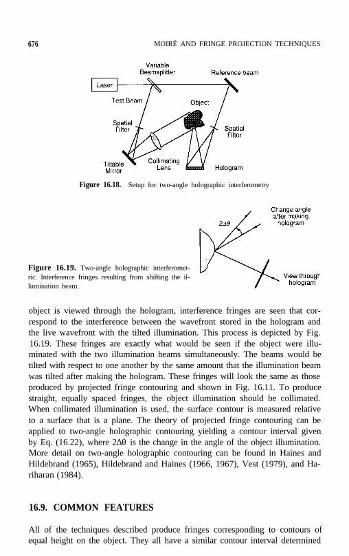
Figure 16.18. Setup for two-angle holographic interferometry

Figure 16.19. Two-angle holographic interferomet-ric. Interference fringes resulting from shifting the il-lumination beam.

object is viewed through the hologram, interference fringes are seen that cor-respond to the interference between the wavefront stored in the hologram andthe live wavefront with the tilted illumination. This process is depicted by Fig.16.19. These fringes are exactly what would be seen if the object were illu-minated with the two illumination beams simultaneously. The beams would betilted with respect to one another by the same amount that the illumination beamwas tilted after making the hologram. These fringes will look the same as thoseproduced by projected fringe contouring and shown in Fig. 16.11. To producestraight, equally spaced fringes, the object illumination should be collimated.When collimated illumination is used, the surface contour is measured relativeto a surface that is a plane. The theory of projected fringe contouring can beapplied to two-angle holographic contouring yielding a contour interval givenby Eq. (16.22), where 2∆θ is the change in the angle of the object illumination.More detail on two-angle holographic contouring can be found in Haines andHildebrand (1965), Hildebrand and Haines (1966, 1967), Vest (1979), and Ha-riharan (1984).

16.9. COMMON FEATURES

All of the techniques described produce fringes corresponding to contours ofequal height on the object. They all have a similar contour interval determined

16.10. COMPARISON TO CONVENTIONAL INTERFEROMETRY 677

by the fringe spacing or grating period and the angle between the illuminationand viewing directions as long as the illumination and viewing are collimated.Phase shifting can be applied to any of the techniques to produce quantitativeheight information as long as sinusoidal fringes are present at the camera. Thesurface heights measured are relative to a reference surface that is a plane aslong as the fringes or grating lines are straight and equally spaced at the object.The only difference between the moiré techniques and the projected fringes andtwo-angle holography is the change in the location of the reference plane. If thefringes are digitized or phase-measuring interferometry techniques are applied,the reference plane can be changed in the computer mathematically.

The precision of these contouring techniques depends on the number offringes used. When the fringes are digitized using fringe-following techniques,the surface height can be determined to 1/10 of a fringe. If phase measurement isused, the surface heights can be determined to 1/100 of a fringe. Therefore it isadvantageous to use as many fringes as possible. And because a reference planecan easily be changed in a computer, projected fringe contouring is the simplestway to contour an object interferometrically.

16.10. COMPARISON TO CONVENTIONAL INTERFEROMETRY

The measurement of surface contour can be related to making the same mea-surement using a Twyman-Green interferometer assuming a long effectivewavelength. The loci of the lines or fringes projected onto the surface (assumingillumination and viewing at infinity) is given by

(16.31)

where z is the height of the surface at the point y, d is the fringe spacing mea-sured along the y axis, and n is an integer referring to fringe order number. Ifthe same surface were tested using a Twyman-Green interferometer, a brightfringe would be obtained whenever

(16.32)

where λ is the wavelength and γ is the tilt of the reference plane. By comparingEqs. (16.31) and (16.32), it can be seen that they are equivalent as long as

(16.33)

and


where λ effec t i v eis the effective wavelength. The effective wavelength can then

be written as

(16.35)

where C is the contour interval as defined in Eq. (16.20). Thus, contouringusing these techniques is similar to measuring the object in a Twyman-Greeninterferometer using a source with wavelength λ effective.

16.11. APPLICATIONS

These techniques can all be used for displacement measurement or stress anal-ysis as well as for contouring objects. Displacement measurement is performedby comparing the fringe patterns obtained before and after a small movementof the object or before and after applying a load to the object. Because thesensitivity of these tests are variable, they can be used for a larger range ofdisplacements and stresses than the holographic techniques. Differential inter-ferometry comparing two objects or an object and a master can also be per-formed by comparing the two fringe patterns obtained. Finally, time-averagevibration analysis can also be performed with moiré, yielding results similar tothose obtained with time-average holography with a much longer effectivewavelength.

Using phase-measurement techniques, the surface height relative to somereference surface can be obtained quantitatively. If the contour lines are straightand equally spaced in object space, then the reference surface will be a plane.In the computer, any plane (or surface) desired can be subtracted from the sur-face height to yield the surface profile relative to any plane (or surface). Thisis similar to viewing the contour lines through a grating (or deformed grating)to reduce their number. If the contour lines are not straight and equally spaced,the reference surface will be something other than a plane. The reference sur-face can be determined by placing a flat surface at the location of the objectand measuring the surface height. Once this reference surface is measured, itcan be subtracted from subsequent measurements to yield the surface heightrelative to a plane surface. Thus, with the use of phase-measuring interfer-ometry techniques, the surface height can be made relative to any surface andtransformed to surface heights relative to another surface. Taking this one stepfurther, a master component can be compared to a number of test componentsto determine if their shape is within the specification. It should also be pointedout that this measurement is sensitive to a certain direction, and that there maybe areas where data are missing because of shadows on the surface.

As an example, Fig. 16.20 shows the mask of Figs. 16.11 and 16.15 con-

16.11. APPLICATIONS 679

Figure 16.20. Mask measured with projected fringes and phase-measurement interferometry. (a)Isometric plot of measured surface height. (b) Isometric plot after best-fit plane removed. (c) Two-dimensional contour plot of measured surface height. (d) Two-dimensional contour plot after best-fit plane removed. Units on plots are in number of contour intervals. One contour interval is ap-proximately 10 mm. The surface is about 150 mm in diameter.


Figure 16.20. (Continued)

toured using fringe projection and phase-measurement interferometry. Thefringes are produced using a Twyman-Green interferometer with a He-Ne laser.A high-resolution camera with 1320 X 900 pixels and a zoom lens is used toview the fringes. Surface heights are calculated using phase-measurement tech-niques at each detector point. A total of five interferograms were used to cal-culate the surface shown in Fig. 16.20a. The best-fit plane has been subtractedfrom the surface to yield Fig. 16.20b. In this way the reference plane has beenchanged. Figures 16.20c and 16.20d show two-dimensional contour maps ofthe object before and after the best-fit plane is removed. These contours canalso be thought of as the fringes that would be viewed on the object. Figure16.20c shows the fringes without a second grating, and Fig. 16.20d is with a

REFERENCES 681

second reference grating chosen to minimize the fringe spacing. The contourinterval for this example is 10 mm, and the total peak-to-valley height deviationafter the tilt is subtracted is about 30 mm.

16.12. SUMMARY

The techniques of projected fringe contouring, projection moiré, shadow moiré,and two-angle holographic contouring are all similar. They all involve project-ing a pattern of lines or interference fringes onto an object and then viewingthose contour lines from a different direction. In the case of the moiré tech-niques, the contour lines are viewed through a grating to reduce the total numberof fringes. In all of the techniques, the surface height is measured relative to areference surface. The reference surface will be a plane if the projected gratinglines or interference fringes are straight and equally spaced at the object andviewed at infinity or with a telecentric imaging system. The use of the secondgrating in the moiré techniques changes the reference plane but does not affectthe contour interval. The sensitivity of the techniques is a maximum when thecontour lines are viewed at an angle of 90o with respect to the projection di-rection. Quantitative data can be obtained from any of these techniques usingphase-measurement interferometry techniques. The precision of the surface-height measurement will depend on the number of fringes present. Surface-height measurements can be made with a repeatability of 1/100 of a contour intervalrms (root-mean-square). Thus, the number of fringes used should be as manyas can easily be measured by the detection system. The contour interval can bechanged to increase the number of fringes, and once the surface height is cal-culated, a reference surface can be subtracted in the computer to find the surfaceheight relative to any desired surface.

Acknowledgments. The authors acknowledge the support of WYKO Corpo-ration during the preparation of this manuscript.

REFERENCES

Abramson, N., “Sandwich Hologram Interferometry. 3: Contouring,” Appl. Opt.,15(1), 200-205 (1976a).

Abramson, N., “Holographic Contouring by Translation,” Appl. Opt., 15(4), 1018-1022 (1976b).

Bell, B., “Digital Heterodyne Topography,” Ph.D. Dissertation, Optical Sciences Cen-ter, University of Arizona, Tucson, AZ, 1985.


Benoit, P., E. Mathieu, J. Hormier, and A. Thomas, “Characterization and Control ofThree Dimensional Objects Using Fringe Projection Techniques,” Nouv. Rev. Opt.,6(2), 67-86 (1975).

Brooks, R. E. and L. O. Heflinger, “Moiré Gauging Using Optical Interference Pat-terns,” Appl. Opt., 8(5), 935-939 (1969).

Case, S. K., J. A. Jalkio, and R. C. Kim, “3-D Vision System Analysis and Design,”in Three-Dimensional Machine Vision, Takeo Kanade, Ed., Kluwer Academic Pub-lishers, Norwell, MA, 1987, pp. 63-95.

Chiang, F.-P., “Moiré Methods for Contouring, Displacement, Deflection, Slope andCurvature,” Proc. SPIE, 153, 113-l 19 (1978).

Chiang, F.-P., “Moiré Methods of Strain Analysis, ” in Manual on Experimental StressAnalysis, A. S. Kobayashi, Ed., Soc. for Exp. Stress Anal., Brookfield Center, CT,1983, pp. 51-69.

DeMattia, P. and V. Fossati-Bellani, “Holographic Contouring by Displacing the Ob-ject and the Illumination Beam,” Opr. Commun., 26(l), 17-21 (1978).

Der Hovanesian, J. and Y. Y. Yung, “Moiré Contour-Sum Contour-Difference, andVibration Analysis of Arbitrary Objects,” Appl. Opt., 10(12), 2734-2738 (1971).

Dureli, A. J. and V. J. Parks, Moiré Analysis of Strain, Prentice-Hall, Englewood Cliffs,NJ, 1970.

Gasvik, K. J., Optical Metrology, Wiley, Chichester, 1987.Guild, J., The Interference Systems of Crossed Diffraction Gratings, Clarendon Press,

Oxford, 1956.Guild, J., Diffraction Gratings as Measuring Scales, Oxford University Press, London,

1960.Haines, K. and B. P. Hildebrand, “Contour Generation by Wavefront Reconstruction,”

Phys. Lett., 19(l), 10-11 (1965).Halioua, M. and H.-C. Liu, “Optical Three-Dimensional Sensing by Phase Measuring

Profilometry,” Opt. Lasers Eng., 11(3), 185-215 (1989).Hariharan, P., Optical Holography, Cambridge University Press, Cambridge, 1984.Hildebrand, B. P. and K. A. Haines, “The Generation of Three-Dimensional Contour

Maps by Wavefront Reconstruction,” Phys. Lett., 21(4), 422-423 (1966).Hildebrand, B. P. and K. A. Haines, “Multiple-Wavelength and Multiple-Source Ho-

lography Applied to Contour Generation,” J. Opt. Soc. Am., 57(2), 155-162 (1967).Indebetouw , G , “Profile Measurement Using Projection of Running Fringes,” Appl.

Opt., 17(18), 2930-2933 (1978).Ligtenberg, F. K., “The Moiré Method,” Proc. Soc. Exp. Stress Anal. (SESA), 12(2),

83-98 (1955).MacGovem, A. J., “Projected Fringes and Holography,” Appl. Opt., 11(12), 2972-

2974 (1972).Meadows, D. M., W. O. Johnson, and J. B. Allen, “Generation of Surface Contours

by Moiré Patterns,” Appl. Opt., 9(4), 942-947 (1970).Menzel, E., “Comment to the Methods of Contour Holography,” Optik, 40(5), 557-

559 (1974).

REFERENCES 683

Moore, D. T. and B. E. Truax, “Phase-Locked Moiré Fringe Analysis for AutomatedContouring of Diffuse Surfaces,” Appl. Opt., 18(l), 91-96 (1979).

Oster, G. and Y. Nishijima, “Moiré Patterns,” Sci. Amer., 208(5), 54-63 (May 1963).Perrin, J. C. and A. Thomas, “Electronic Processing of Moiré Fringes: Application to

Moiré Topography and Comparison with Photogrammetry,” Appl. Opt., 18(4), 563-574 (1979).

Post, D., “Developments in Moiré Interferometry.” Opt. Eng., 21(3), 458-467 (1982).Rayleigh, Lord, “On the Manufacture and Theory of Diffraction-Gratings,” Phil. Mag.

S.4, 47(310) 81-93 and 193-205 (1874).Reid, G. T., “Moiré Fringes in Metrology,” Opt. Lasers Eng., 5(2), 63-93 (1984a).Reid, G. T., R. C. Rixon, and H. I. Messer, “Absolute and Comparative Measurements

of Three-Dimensional Shape by Pulse Measuring Moiré Topography,” Opt. LaserTech., 16(6), 315-319 (1984b).

Righi, A., “Sui Fenomeni Che si Producono colla Sovrapposizione dei Due Reticoli esopra Alcune Lora Applicazioni: I,” Nuovo Cim., 21, 203-227 (1887).

Rowe, S. H., “Projected Interference Fringes in Holographic Interferometry,” J. Opt.Soc. Am., 61(12), 1599-1603 (1971).

Rowe, S. H. and W. T. Welford, “Surface Topography of Non-Optical Surfaces byProjected Interference Fringes,” Nature, 216(5117), 786-787 (1967).

Shagam, R., “Heterodyne Interferometric Method for Profiling Recorded Moiré Inter-ferograms,” Opt. Eng., 19(6), 806-809 (1980).

Srinivasan, V., H. C. Liu, and M. Halioua, “Automated Phase-Measuring Profilometryof 3-D Diffuse Objects,” Appl. Opt., 23(18), 3015-3108 (1984).

Srinivasan, V., H. C. Liu, and M. Halioua, “Automated Phase-Measuring Profilome-try: A Phase Mapping Approach,” Appl. Opt., 24(2), 185-188 (1985).

Takasaki, H., “Moiré Topography,” Appl. Opt., 9(6), 1467-1472 (1970).Takasaki, H., “Moiré Topography,” Appl. Opt., 12(4), 845-850 (1973).Takeda, M. and K. Mutoh, “Fourier Transform Profilometry for the Automatic Mea-

surement of 3-D Object Shapes,” Appl. Opt., 22(24), 3977-3982 (1983).Takeda, M., H. Ina, and S. Kabayashi, “Fourier-Transform Method of Fringe-Pattern

Analysis for Computer-Based Topography and Interferometry,” J. Opt. Soc. Am.,72(l), 156-160 (1982).

Theocaris, P. S., “Moiré Fringes: A Powerful Measuring Device,” Appl. Mech. Rev.,15(5), 333-339 (1962).

Theocaris, P. S., “Moiré Fringes: A Powerful Measuring Device,” in Applied Me-chanics Surveys, Spartan Books, Washington, D.C., 1966, p. 613-626.

Theocaris, P. S., Moiré Fringes in Strain Analysis, Pergamon Press, Oxford, 1969.Vamer, J. R., “Holographic and Moiré Surface Contouring,” in Holographic Nonde-

structive Testing, R. K. Erf, Ed., Academic Press, Orlando, 1974.Vest, C. M., Holographic Interferometry, Wiley, New York, 1979.Wasowski, J., “Moiré Topographic Maps,” Opt. Commun., 2(7), 321-323 (1970).Webster’s Third New International Dictionary, Merriam-Webster, Springfield, MA,

1981.


Welford, W. T., “Some Applications of Projected Interference Fringes,” Opt. Acta,16(3), 371-376 (1969).

Weller, R. and B. M. Shepherd, “Displacement Measurement by Mechanical Interfer-ometry,” Proc. Soc. Exp. Stress Anal. (SESA), 6(l), 35-38 (1948).

Winther, S. and G. A. Slettemoen, “An ESPI Contouring Technique in Strain Analy-sis,” Proc. SPIE, 473, 44-47 (1983).

Yatagai, T., M. Idesawa, Y. Yamaashi, and M. Suzuki, “Interactive Fringe AnalysisSystem: Applications to Moiré Contourogram and Interferogram,” Opt. Eng., 21(5),901-906 (1982).

ADDITIONAL REFERENCES

Asai, K., “Contouring Method by Moiré Holography,” Jpn. J. Appl. Phys., 16(10),1805-1808 (1977).

Boehnlein, A. J. and K. G. Harding, “Adaptation of a Parallel Architecture Computerto Phase Shifted Moiré Interferometry,” Proc. SPIE, 728, 183-193 (1986).

Burch, J. M., “Photographic Production of Scales for Moiré Fringe Applications,” inOptics in Metrology, Brussels Colloquium, May 6-9, 1958, P. Mollet, Ed., Perga-mon Press, New York, 1960, pp. 361-368.

Cabaj, A., G. Ranninger, and G. Windischbauer, “Shadowless Moiré Topography Usinga Single Source of Light,” Appl. Opt., 13(4), 722-723 (1974).

Chiang, F.-P., “Techniques of Optical Signal Filtering Parallel to the Processing ofMoiré-Fringe Patterns,” Exp. Mech., 9(1l), 523-526 (Nov. 1969).

Cline, H. E., A. S. Holik, and W. E. Lorensen, “Computer-Aided Surface Reconstruc-tion of Interference Contours,” Appl. Opt., 21(24), 4481-4488 (1982).

Cline, H. E., W. E. Lorensen, and A. S. Holik, “Automatic Moiré Contouring,” Appl.Opt., 23(10), 1454-1459 (1984).

Gilbert, J. A., T. D. Dudderar, D. R. Matthys, H. S. Johnson, and R. A. Franzel,“Two-Dimensional Stress Analysis Combining High-Frequency Moiré Measure-ments with Finite-Element Modeling,” Exp. Tech., 11(3), 24-28 (March 1987).

Halioua, M., R. S. Krishnamurthy, H.-C. Liu, and F. P. Chiang, “Automated 360o

Profilometry of 3-D Diffuse Objects,” Appl. Opt., 24(12), 2193-2196 (1985).Harding, K. G., M. Michniewicz, and A. J. Boehnlein, “Small Angle Moiré Contour-

ing,” Proc. SPIE, 850, 166-173 (1987).Idesawa, M., T. Yatagai, and T. Soma, “Scanning Moiré Method and Automatic Mea-

surement of 3-D Shapes,” Appl. Opt., 16(8), 2152-2162 (1977).Indebetouw, G., “A Simple Optical Noncontact Profilometer,” Opt. Eng., 18(l), 63-

66 (1979).Jaerisch, W. and G. Makosch, “Optical Contour Mapping of Surfaces,” Appl. Opt.,

12(7), 1552-1557 (1973).Kobayashi, A., Ed., Handbook on Experimental Mechanics, Prentice-Hall, Englewood

Cliffs, NJ, 1987.

ADDITIONAL REFERENCES 685

Kujawinska, M., “Use of Phase-Stepping Automatic Fringe Analysis in Moiré Inter-ferometry,” Appl. Opt., 26(22), 4712-4714 (1987).

Miles, C. A. and B. S. Speight, “Recording the Shape of Animals by a Moiré Method,”J. Phys. E., Sci. Instrum., 8(9), 773-776 (1975).

Pekelsky, J. R., “Automated Contour Ordering for Moiré Topograms,” Opt. Eng.,26(6), 479-486 (1987).

Reid, G. T., “A Moiré Fringe Alignment Aid,” Opt. Lasers Eng., 4(2), 121-126(1983).

Schltzel, K. and G. Parry, “Real-Time Moiré Measurement of Phase Gradient,” Opt.Actu, 29(11), 144-1445 (1982).

Suzuki, M. and K. Suzuki, “Moiré Topography Using Developed Recording Meth-ods,” Opt. Lasers Eng., 3(l), 59-64 (1982).

Theocaris, P. S., “Isopachic Patterns by the Moiré Method,” Exp. Mech., 4(6), 153-159 (1964).

Toyooka, S. and Y. Iwaasa, “Automatic Profilometry of 3-D Diffuse Objects by SpatialPhase Detection,” Appl. Opt., 25(10), 1630-1633 (1986).

Varman, P. O., “A Moiré System for Producing Numerical Data for the Profile of aTurbine Blade Using a Computer and Video Store,” Opt. Lasers Eng., 5(2), 41-58(1984).

Yatagai, T. and M. Idesawa, “Automatic Fringe Analysis for Moiré Topography,”Opt. Lasers Eng., 3(l), 73-83 (1982).

16.1. introduction - stony brook...

Documents