D-A1SE 164 SOME PROPERTIES OF MAXINUM LIKELIHOOD STRATEVY FOR I/RE-PAIRING BROKEN RAND..(U) OHIO STATE UNIV RESEARCHFOUNDATION COLUIBUS P K GOEL ET AL. JAN 86

UNCLASSIFIED OSURF-716366 RFOSR-TR-87-1176 F/0 12/3 UMIEEE'

4

i0 1220

L 1 5 ..

U ,~ 14

SECRIY LASl; AD-A 186 164 93i FIEUG ( )LJMENTATION PAGE

I&. REPORT SECURITY CLSS F I IN~ b. RESTRICTIVE MARKINGSUNCLASSIFIED Anna____________________a__

2& SCURTY CASSFICAION3. DISTRIBUTION/A VAI LABILITY OF REPORT

_N nllApproved for Public Release; Distribution '

.b. Ofi:LABSIIFICATION/DOWNGRA SCHIEDULE Unlimited

4. PERFORMING ORGANIZATION RV5ORT NUM ~ 5. MONITORING ORGANIZATION REPORT NUMB~R~

u~pAFOSR -Th'- 87-17G& NAME OF PERFORMING ORGANIZATION 5.OFFICE SYMBOL 7&. NAME OF MONITOAING ORGANIZATION

Ohio State University (if appicable)

Research Foundation ________AFOSR,'NM

6c. ADDRESS (City. State and ZIP Cod*) 7b. ADDRESS (City. State and ZIP codel1314 Kinnear Road Bldg. 410Columbus, Ohio 43212 Boiling AFB, DC 20332-6448

I&. NAM" OF FUNOING/SPONSORING 6.OFFICE SYMBOL 9. PROCUREMENT INSTRUMENT IDENTIFICATION NUMBERORGANIZATION (if applicable)

AFOSR 1NM AFOSR-84-0 162Sic. ADDRESS (City. State and ZIP Code) 10. SOURCE OF FUNDING NOS.

Bldg. 410 PROGRAM PROJECT TASK WORK UNIT

Bolling AFB, DC E LE MENT NO. NO. NO. NO. %

tt*TEiingmte Cic 1 1 T49a Itln pef o-rties of 6.1102F 2304 K3

Re-airng roen Random amp e12. PERSONAL AUTHOR(IS)

Prem K. Goel and T. Ramalingam13&. TYPE OF RtEPORT___ 13b. TIME COVERED 114. DATE OF REPORT (Yr.. Mo.* Day) 15. PAGE COUNT

interm FROM 71/84 TO 6/30/861 1985; 11, 151G. SUPPLEMENTARY NOTATION%

17. COSATI CODIES 1. SUBJECT TERMS (Continue On ,wueree it neCeaharY and Identify by block number)FIELD GROUP suB. oR. Matching Problem, Maximum l4 kelihood pairing,xxxxxxx xxxxxxx xxxxxxxxxxxxxx Asymptotic properties, Exchangeability,

46-matching19. ABSTRACT (Conttinue on mrer if neceusery and identify by block numb~er)

Matching data from a bivariate population is considered when observations are availableonly in the form of a broken random sample. In other words, a random sample of n pairsis drawn from the population but the observed data consist of n observations on thesecond component and the n observations on an unknown permutation of the first component *

of the n pairs of data. A maximum likelihood matching strateg- is revisited. Theproportion of approximately correct matches (due to Yahav) is used to evaluate theperformance of the pairing strategy as n-*-. The small sample behavior of thisproportion is studied via a Monte-Carlo simulation in the special case of bivariatenormal parent population,

20. DISTRISUTION/AVAILABILITY OF ABSTRACT 2.ABSTRACT SECURITY CLASSIFICATION

UNCLASSIFIED/UNLIMITED I SAME AS RFT. 0 DTIC USERS C1 INCLASS I F) I-l)22s. NAME OF RESPONSIBLE INDIVIDUAL ~22b TELEPHONE NLAABER 22c OFFICE SYMBOL

Ilncludo Area Code), wBrian W. Woodroofe, Major, USAF INM (202 _767-5025 AF)SR/NM

DD FORM 1473,83 APR EDITION OF I JAN 73 IS OBSOLETE. UNCLAS SI F IED

AFOR.Th. 87-1176

Some Properties of Maximum Likelihood Strategyfor Re-Pairing Broken Random Sample

by Prem K. Goel and T. Ramalingam

The Ohio State University and Northern Illinois University

Technical Report #335

January, 1986

Department of Statistics

'The Ohio State University

jAccesic .:Fr J

DTICTAB'. Una-nrouced ['j J sti C: It '

Av,,: .)t~,,j, C r

" " ' "" 102

-, 17 T 7t V W VWW-1

Some Properties of Maximum Likelihood Strategyfor Re-Pairing Broken Random Sample'

By Prem K. Goel & T. RamalingamThe Ohio State University and Northern Illinois University.

Abstract

Matching data from a bivariate population is considered when observations areavailable only in the form of a broken random sample. In other words, a randomsample of n pairs is drawn from the population but the observed data consist of nobservations on the second component and the n observations on an unknownpermutation of the first component of the n pairs of data. A maximum likelihoodmatching strategy is revisited. The proportion of approximately correct matches (dueto Yahav) is used to evaluate the performance of the pairing strategy as n-4 .. Thesmall sample behavior of this proportion is studied via a Monte-Carlo simulation in thespecial case of bivariate normal parent population.

Keywords and Phrases: Matching Problem, Maximum likelihood pairing,asymptotic properties, exchangeability, e -matching,

'This work was supported in part by The National Science Foundation under grantnumber DMS-8400687 and by The Air Force Office of Scientific Research underContract number AFOSR-84-0162.

Some Properties of Maximum Likelihood Strategyfor Re-Pairing Broken Random Sample

By Prem K. Goel & T. RamalingamThe Ohio State University and Northern Illinois University.

1. Introduction. An important tool for analyzing economic policies is themicroanalytic model. Many Federal agencies use such models for the evaluation ofpolicy proposals. When all the input-data for the model come from a single source,the quality of the model depend on, among others, how complete the information is onjointly observed variables. Often times, the input for the model consists of data frommore than one Federal Agency. For instance, to make-up for 'gaps' that occur indecennial Census, the Bureau of the Census and the Internal Revenue Serviceprovide marginal information on variables. However, joint information on thesevariables is not available to either of the two agencies. In such cases, Federalstatisticians use file merging methodology in order to produce comprehensive data onvariables of interest. A review of the origin, progress and recent developments of thismethodology is given in Radner et al (1980).

An unified frame work for all such models for the file-merging methodology andstatistical properties of some of them are given in Ramalingam (1985) and Goel andRamalingam (1985). One useful model for obtaining matched pairs, introduced byDeGroot, Feder and Goel (1971) is as follows: Let W i = (Ti, Ui), i=1,2 .... n be lid

random vectors which are not observable as (t, u) pairs. Instead,it is assumed that themarginal data on t and u are available on these n individuals as follows.

File 1: x , x2 ......... Xn, which is an unknown permutation of the unobservedvalues t1 ,..,t n

File 2: Ul, U?,..,Un

Thus data in File 1 is available at one agency and the data in File 2 is availableat the other agency. Clearly , what is missing from the conceptually unobserved valueson (t,u) is the pairing which, identifies the ti and ui that pertain to the same individual.

DeGroot, Feder and Goel (1971), call the marginal observed data x1 ,..,xn ; u1 ... un a

Broken Random Sample from the population of (T,U).

A In this paper, we shall derive some statistical properties of known stategies to

merge Filel and File 2 in order to reconstruct paired data on (Ti,Ui) for the bivariate

matching problem in which both T and U are one-dimensional variables. We shallbegin with some notations.

1.1 Notations. Let (T,U) have an absolutely continuous joint CDF H(t,u) and jointdensity h(t,u). The marginal dis'ribution functions of T and U will be denoted by G(and F( . ) respectively and I [.] wA denote the indicator function of the event.

-" " , .- - ".'-" " *" * " "'- % % " - *',"% %1% %- k- ... - .

2

Let Gn (x) = (1/n) ,i I [Ti < x] denote the empirical CDF based on thevariables T1 ,..., Tn. Similarly, Fn (x) denotes the empirical COF based on U1 ,..., Un.

Let R(i) = _ I [T i -- T oc I denote the rank of Ti ,i=1,2,...,n. Similarly S(1 ) ..., S(n)denote the ranks of the variables U1,U2, ...,U n .

Let (p = ( p(l),..., p(n) ) be a permutation of the integers 1,2,...,n. The set of all n!permutations of 1,2,... ,n will be denoted by T. Let p* = (1,2, ... , n) denote the identitypermutation.

Let c > 0. For all i= 1,2,... n, and (PET define events Ani (p , - )and Ani (E ) as

follows:

Ani(, ) { U( (R(i)))-U I <5 }. (1.1)

Ani (e) Ani (T *,) (1.2)

For all 1 j,k< n, let

ljk I[Uj-Uk>- cl-I [Tj-Tk>0], (1.3)

2jk I[Tj-Tk>0]- I[Uj-Uk>-e], (1.4)

and 01 =d 02 denotes that the vectors 51and 02 have identical distributions.

2. A Class of Matching Problems. Suppose that h(t,u) has the monotonelikelihood ratio (MLR) property. That is, for all reals tl < t2 and ul < u2 , we have

h(tl, ul) h(t2 , u2)> h(tl,u 2) h(t2 ,ul). (2.1)

If the broken random sample x1 ,... Xn,U. un comes from h(t,u), a typical'matching strategy' based on permutation p r T can be described by pairing x(i )with

u((,(i)). Generalizing the results of DeGroot,Feder & Goel (1971), Chew (1973) showedthat if the MLR property (2.1) holds, then the strategy which maximizes the likelihood[1, h(xi,u(,(i)) of the parameter p over 4', is to pair the ith smallest x with the ith smallestu. Note that, though the pairings in the unobserved sample (Ti,Ui), i=1,2, ..., n areunavailable, the order-statistics of the marginal data on X and U are respectively the

-A ,4

W1J1W~~rV1__VR_%FJ r%- -1,V _VZ W Ww -Nr

same as the ordered values of T and U . Hence, we can write the mergeo file on (T,U)due to any strategy q as

(T (i), U (9 (i)) ,2,...,n (2.2)

Consequently, tht. irged file based on the maximum likelihood pairing (MLP)mentioned above, is obtained by letting cp = (p in (2.2).

Quality of the Merged File. Ideally, we would like to select a (p for whicn tne filein (2.2) recovers all (T,U) pairs in the original unobserved data. It is therefore natural toconsider the random variable N ( p), the number of correct matches due to (P, as anindicator of the performance of the matching (merging) strategy p. The optimraiity of 9°

subject to various criteria, e.g., maximizing the expected number of correct matches,E (N( q))), is discussed in Ramalingam (1985).

Situations often arise where it is not crucial that, after the two files are merged,the matched pairs be exactly the same as the pairs of the original data. For example,when contingency tables analyses are contemplated for grouped data on continuousvariables T and U then, in the absence of the knowledge of the pairings, we would liketo reconstruct the pairs but would not worry too much as long as the u-value in anymatched pair came within a pre-fixed tolerance E (a non-negative number) of the trueu-value that we would get with the ideal matching which recovers all the original pairs.This type of 'approximate matching' was first introduced by Yahav (1982) who definede -correct matching as follows.

Definition 1 (Yahav) . A pair (x(i),u(e(i))), 1 in the merged file (2.2), is said to be V -

correct, if I U(9 (i)) - U[i] I < c, where E > 0 and U[i] is the concomitant of X(i); that is thetrue u-value that was paired with T(i) in the original sample.

The number of e -correct matches N ((p, c), in the merged file (2.2) is given bx

N( (, r ) = ,-i I [ I U(,p (i)) -U[i] I -c ] (2.3)

Note that as c . 0, N(4p,£) converges (almost surely) to N(p) ,the numbe if exactmatches.

The counts N(9p) and N(9,:) are useful indices reflecting the re' oility of the

*merged file (2.2) resulting from (p. We shall now derive some statistic, properties of" N(9p *,c ) In. In view of the fact that Federal files often consist of a 'rge number of

records, it is clear that these asymptotic investigations are useful.

S

3. Asymptotic behavior of N(q)*,E). We first establish a representation for N(q4,r)as a sum of exchangeable 0 -1 random variables. This representation will lead to aneasy proof of the convergence in probability of the proportion, N(9P*,c) /n, of C -correctmatches due to MLP strategy. The following Lemma(See Randles and Wolfe (1979),Theorem 1.3.7, page 16) will be needed.

Lemma 1. If . =d v and K (.) is a measurable function (possibly vector valued) definedon the common support of these random vectors, then K( ) =d K(v)

Proposition 1. Let Ani(T ,e) and N(q ,c) be given by (1.1) and (2.3) respectively. Then,for all (pe 'P

N(p ,E) = - I [Ani(P,)] (3.1)where the summands, I [Ani(P ,c)] are exchangeable binary variables.

Proof. The order-statistic U(, (i)) and the concomitant U[i] of T(i) used in (2.3) can bewritten in terms of the ranks of T's and U's as follows:

U(,p (i)) = Y_ (x Uoc I [R2ox =(P (i)] (3.2)

U[i ] = a U (x I[R1l( = i] (3.3)

Note that N(9p,c ) is simply a count of how many pairs in the merged file based on (P, asdefined in (2.2), satisfy

I U((p(i)) - U[i] I <E. (3.4)

If (3.4) holds for some i, then 3 a j such that

I U ( (i)) - Uj I < E:. (3.5)

In view of the continuity of (Ti,Ui), this correspondence is one-to-one. Therefore, thecount N((p, - ) is same as the count given by

N (p, c)=X(, I U(o(R( U)))-U .. I ] (3.6)

Hence, (3.1) follows from (3.6) and the definition of Ani, in (1.1).

5

In order to show the exchangeability of the summands in (3.1), note that theoriginal samples are independent and identically distributed vectors. Therefore

Wa (1), Wa (2) ...,Wa (n) }=d { Wl ,W2 ... ,Wn } (3.7)

where ( a ](), a(2), ... oc(n) ) is an arbitrary permutation of (1,2,..., n).

Define a function f (f 1 ,f2 .. fn) from i2n to n by

1 ifT-i lI [b j - b i >__ ]< q(ZitI[aj - a-i _> 0 ) _< Il [b j - b i > -

f = (3.8)0 otherwise,

for j=1,2,...,n, where (al,bl, ..., an,bn) is an arbitrary point in -.2n and p e P.lt follows

from (3.7) and Lemma 1 that

f (Wa (1), Wa (2) .... W (n)) =d f (W1 ,W2,...,Wn ) (3.9)

Fix j e {1,2,...,n}. Then, using (3.8), we see that fj (Wa (1), Wo (2) ....Wx (n) ) is theindicator function of the event

I IUa (j)-Ui c ] (p(Xi I [T( j) Ti O] ) i I[Ua (j) - Ui > -c

or, equivalently, in terms of the ranks R1 1.... R1 n of the T's and the empirical CDFGn (.) of U's,

Gn (U(a (j) - C ) < (((Rloa(j))/n < Gn (U o(j) + c ).

Since Gn - 1 (k /n) = U(k) , k=1 ,2,...,n, it follows that fj (Wc (1), Wa (2) .... ,Wu (n) ) is 1 iffIU (p (R a(j)) U a (j)1 5 c. Consequently,

fj (Wa (1), Wa( 2) ,....Wa(n) ) = I [Ana (j) (9,)]. (3.1Oa)Similarly,

fj (W1 ...... Wn) = I [Anj (pc)]. (3.1Ob)

The exchangeability of the summands in (3.1) follows from (3.9), (3.10a) and (3.10b).

We shall now review some results concerning E [N (c )/n], due to Yahav (1982),where N(c ) N (p *,c). Assuming that the distribution of T and U satisfies:

the conditional distribution of U given that T=t is (univariate) normal withmean t and variance 1,

Yahav (1982) derived the limiting value of Pn (c )=E [N (c )/n] as n - by using therepresentation (2.3) in which the summands are functions of the order-statistics of

- A r W -YY h.[ Il

6

U1 ..... Un and the concomitants of the order-statistics of T 1 ..., Tn. His proof relied onan approximation theorem, about the order-statistics for the above model, given inBickel and Yahav(1977). Furthermore, he also reported the findings of a Monte-Carlostudy for ln(C ) in a particular case of his model, namely, T and U are bivariate normalwith correlation p.

We now establish the large-sample behavior of N (c )/n in case of samples froman arbitrary population. The properties of its expected value follow as a consequence.In section 4, we indicate how Yahav's simulation study of the small-sample propertiesof [n(v ) can be improved upon. We shall then present the results of our Monte-Carlo

study of i.tn(c ) when n is small.

Theorem 1. For broken random samples from an absolutely continuous distribution,

N(c )!n- pr 1 (E as n-o (3.11)where

p (c) P[ G(U- c ) < F(T) _< G(U+ c)] (3.12)

Proof: Let Ln = N (c )/n. Using the definitions of Ani(E ) in (1.2) and the representation(3.1) for N (c) as a sum of exchangeable binary variables we obtain

N(£)= _iI [Ani(C)]. (3.13)It follows that

E (Ln) = n P (An1(c ))/n = P (Anl(1 )). (3.14)

Note that

E (Ln2) = n -2 [ E(N(c )) (2) + E (N( ))] (3.15)

where E (N(c )) (2) is the second factorial moment of N(c ). Using the representation(3.13), we get

E (Ln2 ) = n -2 [n( 2 ) P{ Ani (c) An2(c ) }+n P(Anl(c ))].

For cy. =1,2.._n, and j=1 ,2 let

V > _ jcxi (3.16)

where the sequences {l o} and { 2oc} are defined in (1.3) and (1.4). It follows that

Anl(E )=(v11/n< 0, v21/n < 0) (3.17)and

An1 (E )An2(c ) i r)j (v ij/n ! 0). (3.18)

7

Note that, given W 1= (t1 ,u1) ,the infinite sequence 1 12, 1 13.... is exchangeable.Hence, by the Strong Law of Large Numbers for exchangeable random variables (seeChow and Teicher,1978, p.223),

v 1 1/n -- E( 1 12 1 Wl) a.s. as n-

. where the conditional expectation is equal to {G(uj- )- F(tj)}. It follows that

vj, /n --4 G(U 1-e )- F(T1 ) ,a.s. as n -*oo. (3.19)

We can show by similar arguments that

Vla /n -- G(Uoc-E )- F(To ) ,a.s. (3.20)and

v2 x /n -- F(T ) ) G(U a +-c) a.s., (3.21)

where a =1,2. Using the fact (see Serfling, 1980, p.52) that a sequence of vectorsconverges almost surely to a given vector iff the componentwise sequences convergealmost surely to the appropriate components of the limit, we get from (3.20) and (3.21)[ vl /n- [G(U1- c ) -F(T1 )

V21/n F(T1) - G(U 1 + £) a.s. (3.22)

V12 /n G(U 2-e)F( 2)IV2 2 /nL F(T 2 ) - G(U 2 + )j

It follows from (3.17), (3.18), (3.22) and the independence of W 1and W2 that

P(Anl(e ))1 - . (€) (3.23)

andP(Anl (E) An2 (0)) 2 (F) (3.24)

Therefore (3.14), (3.15) and (3.23), (3.24) imply that as n -- oo

E(Ln) - . (C ), (3.25)

and

Var(Ln) --4 0. (3.26)

It is well known that (3.25) and (3.26) imply the convergence in probability as in (3.11).

The following corollary generalizes Yahav's result concerning Pn (c), the firstmoment of N(c )/n.

8

Corollaryl . For p>0, Lp(i) N(c:)/n - (E: as n

(i i) E[ (N(c)/n)P ] - [pj(c)]P as n c,

* Proof: The number of c -correct matches can atmost be n, the number of pairs in theunobserved bivariate-data.Therefore 0 < N(c )/n 5 1, for all n =2,3.... and {N(C )/n} is auniformly bounded sequence of random variables. It is well known that convergence inprobability and Lp-convergence are equivalent for such sequences. Hence (i) follows

easily from Theorem 2. Now, (ii) readily follows from (i) because (I(E )P) is finite forp>0.

Note that in our results, no assumption about the conditional distribution of Ugiven T has been made as was the case with Yahav's results.

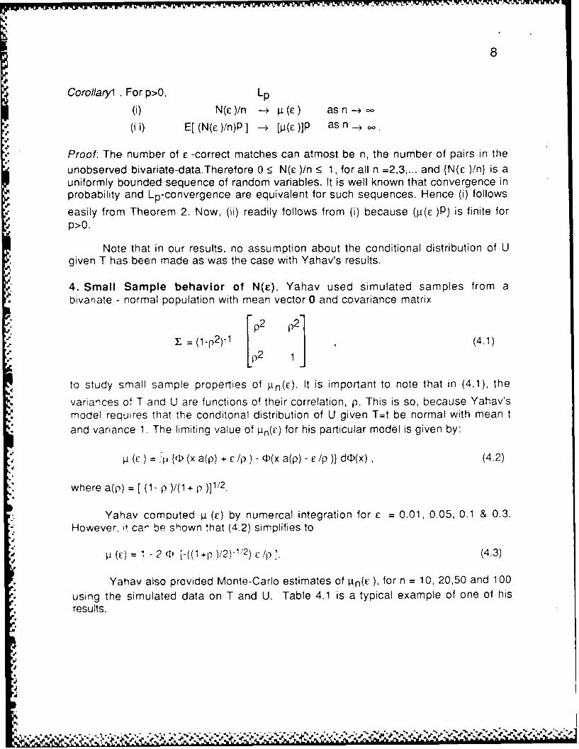
4. Small Sample behavior of N(c). Yahav used simulated samples from abivariate - normal population with mean vector 0 and covariance matrixE 2 p2

= (1-p2 )-1 1 (4.1)p2

to study small sample properties of In(C). It is important to note that in (4.1), thevariances of T and U are functions of their correlation, p. This is so, because Yahav'smodel requires that the conditonal distribution of U given T=t be normal with mean tand variance 1. The limiting value of Pn(c) for his particular model is given by:

4 (v ) =.'p {1( (x a(p) + c/p)- 1(x a(p) - E/p )} dc(x), (4.2)

where a(p) = [ (1- p )/(1+ p )]112 .

Yahav computed ja (c) by numercal integration for £ = 0.01, 0.05, 0.1 & 0.3.However, it can be shown that (4.2) simplifies to

'i (c) = 1 - 2 I [-((1 +p )/2) - 1'2) C /p ]. (4.3)

Yahav also provided Monte-Carlo estimates of 1,1n( ), for n = 10, 20,50 and 100" using the simulated data on T and U. Table 4.1 is a typical example of one of his

results.

J'

9

Table 4.1 Expected Average Number ofE-correct Matchings, e = .01

[Yahav(1 982)]

P P 10(0 P20(0 50() 1 l(£)

.001 .5864 .5326 .5275 .5227

.01 .1984 .1648 .1271 .1152

.10 .1512 .1058 .0760 .0591

.30 .1084 .0686 .0389 .0214

.50 .1020 .0582 .0272 .0138

.70 .0960 .0614 .0262 .,105

.90 .0972 .0540 .0206 .0086

.95 .0976 .0496 .0214 .0083

.99 .0960 .0484 .0213 .0080

It is clear from Table 4.1 and equation (4.3) that Pn (F) and p.(c ) decrease as p

ranges from 0.001 to 0.99. In fact (4.3) implies that t (c)=1-2D(-c) for p =1.0 and p(') =

1.0 for p=0, which goes against the intuition. One expects that for an optimal strategy,such as (p*, Pn(c ) as well as [i(c) must be monotone increasing in p .The problem here

is not with the MLP (p*, but with the covariance matrix Y, defined by (4.1), used inYahav's model. Because, as p changes its value, so do the marginal variances of T

, and U. In fact, as p - 1, the marginal variances -> o. To rectify this problem, we haveassumed a bivariate normal model for T and U with means zero, variances one andthe correlation p

For each combination of four values of n, namely 10, 20, 50 and 100, andtwelve values of p , namely 0.00, 0.10 (0.10) 0.90, 0.95, 0.99; 1000 sample weregenerated from the bivariate normal population using the IMSL Library routines.These data were used to obtain Monte-Carlo estimates of Pn(c ), where C was giventhe values 0.01, 0.05, 0.1, 0.3, 0.5, 0.75, 1.0.

It is easy to show that, for the above model

p. (c) = P(I Z I c v (2(1-p ))-1/2 ), (4.4)

where Z is a standard normal random variable. It is clear from (4.4) that p (C ) is a

monotone increasing function of p. Using standard-normal CDF tables, p- (t: ) in (4.4)

was computed for each combination of the twelve values of p and the seven values of

c mentioned above. The estimated values of P.n () and the limiting value i (c ) are

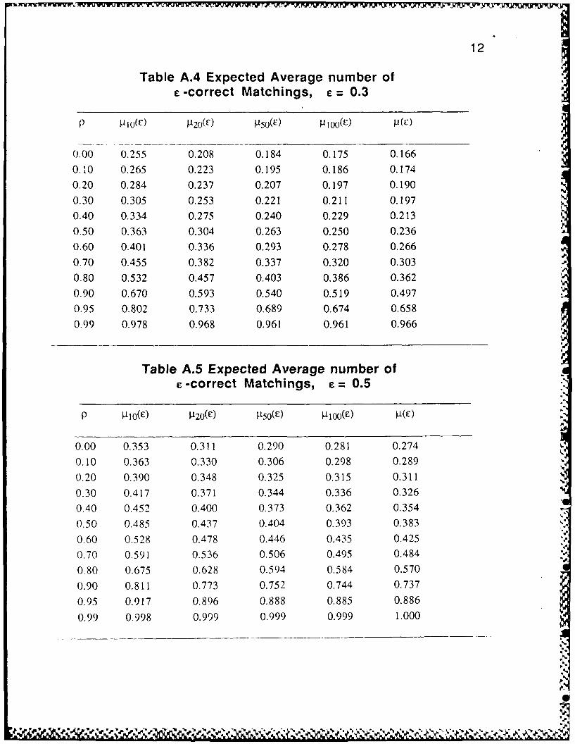
given in Tables A.1-A.7 in the Appendix.

10

Note that, as expected, n(c) and t(E) in Tables A.1-A.7 are monotoneincreasing functions of p for each fixed e. Furthermore, the quality of the merged file is

quite good if we want to reconstruct contingency tables with intervals of size .5 a ormore and the correlation p _ 0.5.

APPENDIX

Table A.1 Expected Average number ofe -correct Matchings, e = 0.01

P 106O(C) 20(04 .50(c) I 1 5 0(C)

0.00 0.106 0.054 0.025 0.015 0.0080.10 0.113 0.059 0.028 0.017 0.0080.20 0.127 0.068 0.031 0.018 0.0080.30 0.138 0.075 0.034 0.020 0.0080.40 0.155 0.083 0.038 0.023 0.0080.50 0.174 0.095 0.044 0.026 0.0080.60 0.199 0.109 0.061 0.036 0.0080.70 0.231 0.129 0.061 0.036 0.0080.80 0.279 0.162 0.077 0.046 0.0160.90 0.374 0.222 0.109 0.067 0.016

0.95 0.476 0.296 0.151 0.094 0.0240.99 0.700 0.521 0.299 0.191 0.056

.1'

'p

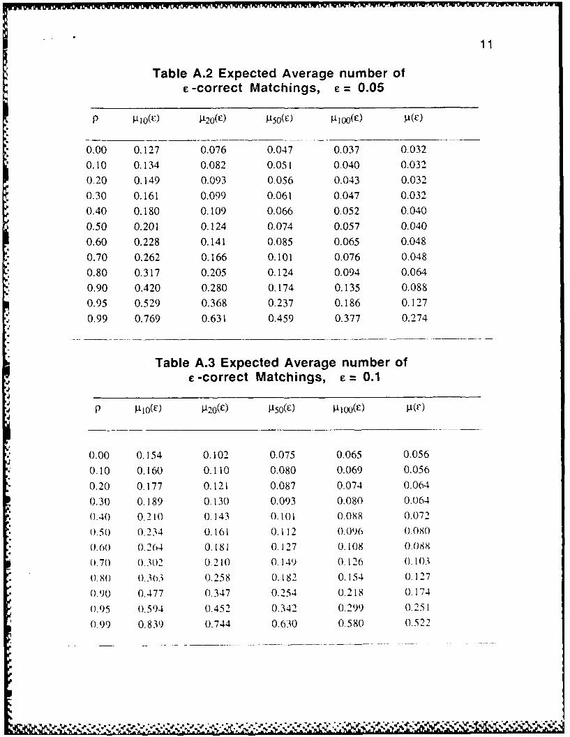
Table A.2 Expected Average number ofe -correct Matchings, c = 0.05

P I O(c) P 20() P50 () 1 O0(E)

0.00 0.127 0.076 0.047 0.037 0.032

0.10 0.134 0.082 0.051 0.040 0.032

0.20 0.149 0.093 0.056 0.043 0.032

0.30 0.161 0.099 0.061 0.047 0.032

0.40 0.180 0.109 0.066 0.052 0.040

0.50 0.201 0.124 0.074 0.057 0.040

0.60 0.228 0.141 0.085 0.065 0.048

0.70 0.262 0.166 0.101 0.076 0.048

0.80 0.317 0.205 0.124 0.094 0.064

0.90 0.420 0.280 0.174 0.135 0.088

0.95 0.529 0.368 0.237 0.186 0.127

0.99 0.769 0.631 0.459 0.377 0.274

Table A.3 Expected Average number ofe -correct Matchings, e = 0.1

P L.Io(C) P,.o( ) laso( ) oo( ) 11()

0.00 0.154 0.102 0.075 0.065 0.056

0.10 0.160 0.110 0.080 0.069 0.056

0.20 0.177 0.121 0.087 0.074 0.064

0.30 0.189 0.130 0.093 0.080 0.064

0.40 0.210 0.143 0.101 0.088 0.072

0.50 0.234 0.161 0.112 0.096 0.080

0.60 0.264 0.181 0. 127 0.108 0.088

0.70 0.302 0.210 0.149 0.126 0.103

0.80 0.303 0.258 0.182 0.154 0.127

0.90 0.477 0.347 0.254 0.218 0.174

0.95 0.594 0.452 0.342 0.299 0.251

0.99 0.839 0.744 0.630 0.580 0.522

**d ~*. ~ ~ ." ~~'-.- s~ -:v b *l%. . . . . -. . . . . . .. V_.

12

Table A.4 Expected Average number of- -correct Matchings, c = 0.3

) p I o(V) P1-)o(C) P50(0 P Ij (c) P (c)

0.00 0.255 0.208 0.184 0.175 0.166

0.10 0.265 0.223 0.195 0.186 0.174

0.20 0.284 0.237 0.207 0.197 0.190

0.30 0.305 0.253 0.221 0.211 0.197

0.40 0.334 0.275 0.240 0.229 0.213

0.50 0.363 0.304 0.263 0.250 0.236

0.60 0.401 0.336 0.293 0.278 0.266

0.70 0.455 0.382 0.337 0.320 0.3030.80 0.532 0.457 0.403 0.386 0.3620.90 0.670 0.593 0.540 0.519 0.4970.95 0.802 0.733 0.689 0.674 0.658

0.99 0.978 0.968 0.961 0.961 0.966

Table A.5 Expected Average number of

c -correct Matchings, £ = 0.5

p ().10(E) .t50 () PI00(E) WO

0.00 0.353 0.311 0.290 0.281 0.274

0.10 0.363 0.330 0.306 0.298 0.289

0.20 0.390 0.348 0.325 0.315 0.311

0.30 0.417 0.371 0.344 0.336 0.326

0.40 0.452 0.400 0.373 0.362 0.354

0.50 0.485 0.437 0.404 0.393 0.383

0.60 0.528 0.478 0.446 0.435 0.425

0.70 0.591 0.536 0.506 0.495 0.484

0.80 0.675 0.628 0.594 0.584 0.570

0.90 0.811 0.773 0.752 0.744 0.737

0.95 0.917 0.896 0.888 0.885 0.886

0.99 0.998 0.999 0.999 0.999 1.000

p .

41 f ~ ~ %1B~~ -

13

Table A.6 Expected Average number of,e -correct Matchings, e = 0.75

P I O(E) .2 0 () ) ( 10 0 (e) ()

0.00 0.468 0.433 0.416 0.409 0.404

0.10 0.488 0.454 0.437 0.429 0.425

0.20 0.514 0,477 0.461 0.453 0.445

0.30 0.539 0.505 0.487 0.480 0.471

0.40 0.582 0.542 0.522 0.514 0.503

0.50 0.621 0.586 0.560 0.555 0.547

0.60 0.662 0.633 0.613 0.606 0.59-,j

0.70 0.727 0.694 0.679 0.673 0.668

0.80 0.810 0.786 0.772 0.768 0.766

0.90 0.919 0.908 0.906 0.904 0.907

0.95 0.979 0.976 0.978 0.979 0.982

0.99 1.000 1.000 1.000 1.000 1.000

Table A.7 Expected Average number ofe-correct Matchings, e= 1.0

P PIo(O) t2o(0) '5o(0 ) 0to(c) WO

0.00 0.570 0.545 0.531 0.524 0.522

0.10 0.593 0.566 0.555 0.549 0.547

0.20 0.621 0.595 0.581 0.576 0.570

0.30 0.646 0.622 0.611 0.605 0.605

0.40 0.690 0.664 0.650 0.644 0.627

0.50 0.729 0.707 0.691 0.688 0.683

0.60 0.772 0.753 0.744 0.741 0.737

0.70 0.830 0.812 0.807 0.805 0.803

0.80 0.898 0.889 0.887 0.885 0.886

0.90 0.970 0.970 0.972 0.972 0.975

0.95 0.996 0.996 0.997 0.997 0.998

0.99 1.000 1.000 1.000 1.000 1.000

.9

.,,

Sa

• ++ 5 55 *-] . II k S i - A t~ ~ :'~ S* ' 5 . ", J .. ,1 l tl,.:, .- -l ll5~t J,

14

REFERENCES

Bickel, P.J and Yahav, J.A. (1977) On Selecting a Subset of Good Populations, inStatistical Decision Theory and Related Topics II, (Eds.) S. S. Gupta and D.S. Moore,Academic Press, New York.

Chow, Y.S and Teicher, H.(1978) Probability Theory, Springer-Verlag, New York.

Chew, M.C (1973), On Pairing Observations from a Distribution with MonotoneLikelihood Ratio, Annals of Statistics, 1 , 433-445.

DeGroot, M.H, Feder, P.I., Goel, P.K. (1971), Matchmaking, Annals of MathematicalStatistics, 42, 578-593.

Goel, P.K. & Ramalingam, T. (1985) The Matching Methodology:Some StatisticalProperties,Technical Report # 333,Department of Statistics,Ohio State University

Radner, D.B. et. al (1980), Report on Exact and Statistical Matching Techniques,Statistical Policy Working Paper No. 5, Office of Federal Statistical Policy andStandards, U.S. Dept. of Commerce.

Ramalingam, T (1985): Statistical Properties of the File-merging Methodology, Ph.D.Thesis, Purdue University

Randles, R.H and Wolfe, D.A (1979), Introduction to the Theory of NonparametricStatistics, John Wiley, New York.

Serfling, R.J (1980), Approximation Theorems of Mathematical Statistics, John Wiley,New York.

Yahav, J. A. (1982), On Matchmaking, in Statistical Decision Theory and Related* Topics III, vol 2.,(Eds.) S.S. Gupta and J.O. Berger,497-504 Academic Press, New*: York.

4k,?,.Ile ",. ,. )

,, 1t.."0 .,.. .,*

S ,t ,-",,,'.c,/4." 1O '4,. C

kt3f T'eZev

4k

doomp

06

55-.