Data Editing and Imputation

Prepared by:

Tamara BlackJohn CoderNathan ConverseVeronica Cox

Report No. 10

An Urban InstituteProgram to AssessChanging Social Policies

Assessingthe NewFederalism

Meth

odology

Rep

ortsNSAF

Aparna Lhila Fritz Scheuren Urban Institute

Sarah Dipko Michael Skinner Nancy Vaden-Kiernan Westat

Data Editing and Imputation

1999 NSAF1999 NSAF

Preface 1999 NSAF Data Editing and Imputation is the tenth report in a series describing the methodology of the 1999 National Survey of America's Families (NSAF). It is a companion to the recently reissued 1997 NSAF Report on the same topic (No. 10 in that series). This is a reissued version of the 1999 NSAF report No. 10 that incorporates the changes and edits made by the Urban Institute’s Survey Associate Timothy Triplett. About the National Survey of America’s Families (NSAF) As discussed elsewhere (e.g., see especially Report No. 1 in the 1997 NSAF methodology series), NSAF is part of the Assessing the New Federalism Project at the Urban Institute, being done in partnership with Child Trends. Data collection for the NSAF was conducted by Westat. In each rounds of NSAF, carried out so far, over 40,000 households were interviewed, yielding information on over 100,000 people. NSAF has focused on the economic, health, and social characteristics of children, adults under the age of 65, and their families. The sample is representative of the nation as a whole and of 13 states. Because of its large state sample sizes, NSAF has an unprecedented ability to measure differences between the 13 states it targeted. About the 1997 and 1999 NSAF Methodology Series The 1997 and 1999 methodology series of reports have been developed to provide readers with a detailed description of the methods employed to conduct the 1997 NSAF. The two series are nearly parallel, except for the documentation of the public use files, where an on-line system is being developed for the 1999 survey and we are planning to reissue the 1997 files using this on-line documentation system. Report No. 1 in the 1997 series introduces NSAF. Report Nos. 2 through 4 in both series—plus Report No. 14 in the 1997 series—describe the sample design, how survey results were estimated and how variances were calculated. Report Nos. 5 and 9 in each series describe the interviewing done in for the telephone (RDD) and in-person samples. Report Nos. 6 and 15 in the 1997 series and Report No. 6 in the 1999 series displays and discusses the comparisons we made to surveys that partially overlapped NSAF in content—including the Current Population Survey and the National Health Interview Survey, among others. Report Nos. 7 and 8 in both series cover what we know about nonresponse rates and nonresponse biases. Report No. 10 in both series covers the details of the survey processing, after the fieldwork was completed, including the imputation done for items that were missing. Report No. 11 in both series introduces the public use files made available. In the 1997 series, there were additional reports on the public use files available in a PDF format as Report No. 13, 17-22. These will all eventually be superceded by the on-line data file codebook system that we are going to employ for the 1999 survey. The 1997 and 1999 NSAF questionnaires are available respectively as Report No. 12 in the 1997 series and Report No. 1 in the 1999 series. Report No. 16 for the 1997 series, the only report not so far mentioned contains

occasional papers of methodological interest given at professional meetings through 1999, regarding the NSAF work as it has progressed over the years since 1996 when the project began. About this 1999 Report Report No. 10 focuses on data editing techniques, including data processing, how data errors were dealt with, how edits were made, and coding guidelines, as well as how data were “filled in” when values were missing and editing that was done to protect confidentiality. Some discussion is also provided of the relative size of sampling variance to mean square error. For More Information For more information about the National Survey of America's Families, contact Assessing the New Federalism, Urban Institute, 2100 M Street, NW, Washington, DC 20037, telephone: (202) 261-5886, fax: (202) 293-1918, Website: http://newfederalism.urban.org. Kevin Wang And Fritz Scheuren

i

Table of Contents Chapter Page

1 Overview of Data Editing and Item Imputation....................................................... 1-1

1.1 Introduction .................................................................................................. 1-1 1.2 Data Editing and Data Coding (Chapters 2 and 3)............................................. 1-1 1.3 Item Imputation (Chapter 4) ............................................................................. 1-2 1.4 Analytic Concerns and Implications ................................................................. 1-4

2 Data Editing .................................................................................................. 2-1

2.1 Introduction .................................................................................................. 2-1 2.2 Problem Cases .................................................................................................. 2-2

2.2.1 Communication of Problems................................................................. 2-2 2.2.2 Classification of Problem Sheets ........................................................... 2-2 2.2.3 Round 2 Production Account Problem Sheets ....................................... 2-3 2.2.4 Comparison of Round 2 with Round 1 Problem Sheets ......................... 2-4

2.3 Problems Recorded in the Electronic Queue ..................................................... 2-4 2.3.1 Volume of Electronic Queue Problems ................................................. 2-5 2.3.2 Comparison of Round 2 with Round 1 Electronic Problems, Discussion of Volume Over Time ......................................................... 2-6

2.4 Overall Volume of Problem Cases.................................................................... 2-8 2.5 Problem Resolutions......................................................................................... 2-9 2.6 Addition of NOTES Coding and Description of Results ................................. 2-10

2.6.1 NOTES Types and Basic Counts......................................................... 2-10 2.6.2 NOTES Types Summarized by Major Groups, by Questionnaire Level ............................................................................ 2-12 2.6.3 NOTES Communication Sources by Questionnaire Level ................... 2-13 2.6.4 NOTES in Households........................................................................ 2-14

2.7 Comparison of Problems in Round 1 and Round 2.......................................... 2-14 2.8 Summary ................................................................................................ 2-15 2.9 Comments ................................................................................................ 2-16

2.9.1 Comment Review ............................................................................... 2-16 2.9.2 Use of Comments from Completes to Reinforce Training Issues ......... 2-16 2.9.3 Summary ............................................................................................ 2-17

2.10 Coding ................................................................................................ 2-17 2.11 Quality Control............................................................................................... 2-18

2.11.1 Limiting the Number of Staff Who Made Updates .............................. 2-18 2.11.2 Using Flowcharts ................................................................................ 2-18 2.11.3 Using CATI Program to Ensure Clean Data ........................................ 2-18 2.11.4 Monthly Data Deliveries ..................................................................... 2-19 2.11.5 Programmatic Checks ......................................................................... 2-19 2.11.6 Interactive Resolution of Updates to Completed Interview Roster Data for Consistency with Round 1.......................................... 2-20

2.12 Editing for Confidentiality .............................................................................. 2-22 2.12.1 Constructing New Variables ............................................................... 2-22 2.12.2 Top and Bottom Coding and Data Blurring ........................................ 2-23

ii

Table of Contents

Chapter Page

3 Data Coding .................................................................................................. 3-1

3.1 Introduction to Data Coding and Review .......................................................... 3-1 3.1.1 Coding Other Specify Variables............................................................ 3-1 3.1.2 The Look-Up Table .............................................................................. 3-1 3.1.3 Matching Misspelled or Grammatically Incorrect Data in Look-up ....... 3-2 3.1.4 The Matching Process........................................................................... 3-5 3.1.5 Developing Coding Guidelines ............................................................. 3-6 3.1.6 Reviewing Data in Access..................................................................... 3-8

3.2 Summary… … … ............................................................................................ 3-10

Chapter Page

4 Data Imputation .................................................................................................. 4-1

4.1 Introduction .................................................................................................. 4-1 4.2 Hot Deck Imputation In General ....................................................................... 4-1 4.3 NSAF Sections Imputed Using Hot Deck Imputation ....................................... 4-3

4.3.1 Imputation for Income and Employment ............................................... 4-3 4.3.2 Imputation for Health Insurance and Health Care Utilization ................ 4-3 4.3.3 Imputation for Housing and Economic Hardship................................... 4-3

4.4 Detailed Imputation Procedures........................................................................ 4-4 4.4.1 Section I: Employment Questions ......................................................... 4-4 4.4.2 Section J: Transfer Programs and Other Unearned Sources ................... 4-5 4.4.3 Sections E and F Health Care Imputations............................................. 4-6 4.4.4 Section M Imputations .......................................................................... 4-7

4.5 Comparing Imputed Values with Reported Values............................................ 4-7 4.6 Imputation Impact on Variance Estimation and Inference Generally ............... 4-10

References .... ........... .......... ................................................................................................. A-1

iii

List of Tables

Table Title Page Table 2-1. Categories Used to Classify Problem Sheets ..................................................... 2-3 Table 2-2. Round 2 Problem Sheet Summary and Comparison to Round 1........................ 2-4 Table 2-3. Round 2 Electronic Problems, by Questionnaire Level and Result Code, and Comparison to Round 1 ............................................................................. 2-5 Table 2-4. Cycle 2 Summary of Electronically-Coded Problems (8’s) by Month and Comparison to Cycle 1............................................................... 2-7 Table 2-5. Overall Volume of Problem Cases.................................................................... 2-8 Table 2-6. Electronic Problems in Households, by Questionnaire Level, Including 8’s, 82’s, 83’s ................................................................................... 2-8 Table 2-7. NOTES Types and Descriptions, with Basic Counts by Type Code ................ 2-11 Table 2-8. NOTES Grouped by Type, by Questionnaire Level ........................................ 2-12 Table 2-9. NOTES by Source of Problem Communication to Data Prep Staff and

Questionnaire Level ....................................................................................... 2-13 Table 2-10. NOTES in Households, by Questionnaire Level ............................................. 2-14 Table 2-11. Summary of Interactive Case Review Performed for Urban Institute .............. 2-21 Table 4.5.1 CPS Education Level: Reported in Both Rounds .............................................. 4-8 Table 4.5.2 CPS Education Level: Reported Once, Imputed Once....................................... 4-8 Table 4.5.3 Additional Telephones for Nonbusiness Use: Reported Both Rounds ............... 4-9 Table 4.5.4 Additional Telephones for Nonbusiness Use: Reported Once, Imputed Once .................................................................................................. 4-9

List of Figures Figure Title Page Figure 2-1. Cycle 2 Problem 8's by Questionnaire Level and Comparison to Cycle 1 Totals......................................................................... 2-15 Figure 3-1. Sample Lines from KAWORKD Look-up Table .............................................. 3-2 Figure 3-2. Sample PARMFILE ......................................................................................... 3-4 Figure 4-1...... Variance Adjustments .................................................................................... 4-36

1-1

Chapter 1 Overview of Data Editing and Item Imputation

1.1 Introduction

As discussed in the earlier editing and imputation report on the 1997 NSAF (Report No. 10 in the 1997 series), the National Survey of America’s Families (NSAF) was a first-ever effort, put together quickly to respond to major changes in welfare policy at the federal and state levels. The Urban Institute and Child Trends, who jointly led the effort, combined their expertise with the efforts of Westat, an experienced survey firm. Together, the ingredients were present for a successful endeavor. Still, there were many (mostly expected) difficulties, along with some unexpected developments. By the second (1999) round of NSAF, many of the survey-data-handling problems encountered in the first round had been "solved." We were able to repeat, therefore, our (often hard won) approaches, making refinements where possible and documenting what we did more thoroughly. The present report benefits from this growing experience in two ways. First, much of what we did is not new and we, therefore, will repeatedly refer the reader back to the parallel 1997 report. On the other hand, users of the 1997 round of NSAF may find profit here, too, because we consciously tried to keep consistency between rounds wherever possible. And some aspects of what was done in the first round, notably the handing of the coding of open-ended responses, or "other specifies," are more thoroughly documented here. Because the two rounds were meant to have consistent treatment, we are, in effect, continuing to document the 1997 round. The present report describes what was done to edit the 1999 NSAF data (see chapter 2), to code written-in entries and match the two rounds of the survey (chapter 3), and to impute for missing item information in 1999 (chapter 4). The public-use file documentation for both rounds, of course, adds many important details on individual variables. In the 1997 report on data editing and imputation, we also had a chapter on general analytic implications of the data flaws detected and undetected. Although referenced here, the same ground has not been repeated, except for a few remarks at the end of the present chapter. 1.2 Data Editing and Data Coding (Chapters 2 and 3) As detailed in chapters 2 and 3, the data editing process for the 1999 NSAF consisted of three main tasks: handling problem cases, reading and using interviewer comments to make data updates (chapter 2), and coding questions with text strings (chapter 3). Extensive quality control procedures were implemented to ensure accurate data editing. For the second round of the survey, the work easily separated organizationally into the two activities (editing and coding). Westat did most of the data editing that involved interviewer comments and updates. On the other hand, except for the coding done at the Census Bureau of industry and occupation, all the postsurvey editing and assignment of codes for open-ended questions was done at the Urban Institute.

1-2

Strategies for quickly handling data collection problems were developed by Westat during Round 1 of the NSAF in 1997. This development work made the 1999 survey problem resolution much less time-consuming than it had been during Round 1. The volume of problems in Round 2 was not as high as it had been in Round 1, and the problems were not as complex; hence, they could be resolved more quickly. Better CATI (computer-assisted telephone interviewing) software and an improved questionnaire were the major factors that made the process less difficult. Interviewing for the NSAF was conducted at seven different interviewing facilities that were on slightly different schedules for the beginning of data collection. All comments were read during the first two weeks of data collection at each facility. After this period, only 10 percent of the comments were read. Limited updates were made to interviews based on comments and problem sheets. The purpose of comment review was changed in Round 2 from searching for data updates to alerting the project team of interviewer training weaknesses. Some comments were used when making updates to completed cases identified through other means, such as programmatic checks run by the Urban Institute. If comments were present when interim problem cases were reviewed, these were taken into account in decision-making. During Round 1, but not Round 2, Westat conducted coding for “other specify” and open-ended questions. “Other specify” questions were those in which a question had some specific answer categories but also allowed text to be typed into an "other" category. Open-ended questions had no precoded answer categories. Westat and the Urban Institute had developed an interactive process for defining these codes during Round 1. It was this structure that was built upon in the 1999 survey. Its implementation was done solely at the Urban Institute in Round 2. Often, for "other-specify," we were able to start with the exact decisions made in Round 1 for a respondent comment. Matching these by computer, we were able to ensure complete consistency. Because data editing resulted in updates to the data, careful quality control procedures were implemented, at both Westat and the Urban Institute. These measures involved limiting the number of staff who made updates, using flowcharts to diagram complex questionnaire sections, consulting frequently, carefully checking updates, and conducting computer checks for inconsistencies or illogical patterns in the data. 1.3 Item Imputation(Chapter 4) For most NSAF questions, item nonresponse rates were very low (often less than 1 percent), and seldom did we impute for missing responses. The pattern and amount of missingness from round to round varied very little and our approach was virtually identical. The answers to opinion questions were not imputed for any of the cases. The number of missing entries is available on the public-use files, variable by variable, for most items (see chapter 4 of the parallel 1997 NSAF Report on Data Editing and Imputation).

1-3

Still, there were important questions for which missing NSAF responses were imputed to provide a complete set of data for certain analyses. For example, the determination of poverty status is crucial, but often at least one of the income items that had to be obtained to make this determination was not answered. As is the case in many household surveys, NSAF encountered significant levels of item nonresponse for questions regarding sensitive information such as income, mortgage amounts, health care decisions, and so forth. In fact, the income-item nonresponse could range up to 20 or even 30 percent in the NSAF. Hence, the problem could not be ignored. For an introduction to this literature, see especially Kalton (1983), Little and Rubin (1987), Lyberg and Kaspryzk (1997). The three volumes of Incomplete Data in Sample Surveys (Madow et al., 1983) are still, in many ways, definitive. As will be explained further in chapter 4, the imputation of missing responses is intended to meet two goals. First, it makes the data easier to use. For example, the imputation of missing income responses permits the calculation of total family income (and poverty) measures for all sample families--a requirement to facilitate the derivation of estimates at the state and national levels. Second, imputation helps adjust for biases that may result from differences between persons who responded and those who did not. The approach used to make the imputations for missing responses in the NSAF was “hot deck” imputation (e.g., Ford 1983). In a hot deck imputation, the value reported by a respondent for a particular question is given or donated to a “similar” person who failed to respond to that question. The hot deck approach to imputing missing values is the most common method used to assign values for missing responses in large-scale household surveys. For the NSAF, a hierarchical statistical matching hot deck design was used (Coder, 1999). The first step in this imputation process was the separation of the sample into two groups: those who provided a valid response to an item and those who did not. Next, a number of matching “keys” were derived, based on information available for both respondents and nonrespondents. These matching keys vary according to the amount and detail of information used. One matching key represents the “highest” or most desirable match and is typically made up of the most detailed information. Another matching key is defined to be the “lowest” or least desirable. Additional matching keys are defined to fall somewhere between these two; when combined, these keys make up the matching hierarchy. The matching of respondents and nonrespondents for each item is undertaken based on each matching key. This process begins at the highest (most detailed) level and proceeds downward until all nonrespondents have been matched to a respondent. The response provided by the donor matching at the best (highest) level is assigned or donated to the nonrespondent. For the most part, respondents are chosen from the “pool of donors” without replacement. However, under some circumstances, the same respondent may be used to donate responses to more than one nonrespondent. By design, multiple use of donors is kept to a minimum. An imputation “flag” is provided for each variable handled by the imputation system. In fact, all imputations assigned can be easily tied to the donor through the Donor ID number, because it is retained. The linkages between donor and donee were all kept as part of the complete audit trail

1-4

maintained throughout the process, although they are not currently being made available on the NSAF Public Use Files. 1.4 Analytic Concerns and Implications The NSAF, by its very nature, was long and probing--often asking questions never brought together before in the same instrument. Clearly, the length and complexity of the questionnaire contributed to the challenges to be faced--notably in making the data editing more difficult and the level of item nonresponse greater. Noninterviews have been extensively covered in Reports No. 7 and 8 in the 1997 Methodology Series, plus in selected papers found in Report No. 16 of the 1997 series and Report No. 7 in the 1999 series. Despite the fact that the unit nonresponse was sizable and raised the cost of the survey, there is little evidence of any serious overall bias after adjustment. Although the path through the evidence is different, we believe that the problems of data editing and item nonresponse are similar in their effect. Their existence in NSAF created extra work, but after the adjustments described here, there is little evidence to suggest significant residual biases beyond those normal to household surveys. This point has already been made in Methodology Report No. 1 of the 1997 series and is elaborated on further in Report No. 15 of that series and Report No. 6 of the 1999 series. In both these reports, NSAF is compared directly with the Bureau of the Census’ March Current Population Survey (CPS) and other major national samples. Despite the high quality of the data editing and imputation in the NSAF, researchers still need to be concerned with how they handle the resulting data. Hot deck imputation, for example, increases the sampling error (Scheuren, 1976) in ways that are hard to measure without special procedures, such as multiple imputation (Rubin, 1987). We recommend that analysts of NSAF data, that have been partially imputed, use an adjustment to their standard errors that corrects for the fact that they do not have as many cases as the variance estimation software (e.g., Wesvar) assumes. One conservative approach to this problem is covered in chapter 4, section 4.6, of this report. References to other options are also provided. Misclassification concerns arise in any editing or imputation procedure unless the method of assignment perfectly places each missing or misreported case into the right group. The final analyst might employ a reweighting (or reimputation) option rather than just using the imputations provided. To support this option on the NSAF Public Use Files, we have provided a great deal of diagnostic information including the imputation flags, replicate weights, sampling variables, and some variables associated with the interview process itself (e.g., date of interview, number calls to complete ). As with any data set, researchers will need to be aware of possible anomalies. We believe, however, that these are rare in the NSAF Public Use Files, whether for 1997 or 1999. Still, it is unlikely that we have been able to anticipate all the ways in which the data will be used. Almost certainly there are errors that will be found when researchers carry out their detailed investigations. We would greatly appreciate being informed of any such discrepancies, so they

1-5

can be brought to the attention of others. Furthermore, depending on the nature of this information, new data sets may be made available. To give a context to the NSAF effort, there is a bibliography at the end of this report that includes some useful theoretical references plus citations related to the editing and imputation practices used in similar surveys (see especially the Federal Committee on Statistics Methodology Report on Data Editing, Report No 24).

2-1

Chapter 2 Data Editing

2.1 Introduction The NSAF has had two rounds of data collection. The first was in 1997 (Round 1) and the second was in 1999 (Round 2). This report describes Round 2. For information about data editing in Round 1, see Data Editing and Imputation, Report No. 10 in the 1997 Methodology Series. The data editing conducted by Westat for the Round 2 NSAF consisted of four main tasks: handling problem cases; reading interviewer comments for quality control purposes; making needed changes to interim cases; and making recommendations to the Urban Institute about how to update completed cases with problems. Quality control procedures were implemented to ensure accurate data editing. Interviewers communicated problems cases in two ways, either through a problem sheet or by assigning a special result code. Strategies for handling problems were developed during Round 1 of the NSAF in 1997. This development work made the resolution of problems much less time consuming than it had been during Round 1. The volume of problems in Round 2 was not as high as it had been in Round 1, and the problems were not as complex and could be resolved more quickly. Interviewing for the NSAF was conducted at seven different interviewing facilities that were on slightly different schedules for the beginning of data collection. Comments were read during the first two weeks of data collection at each facility. After this period, 10 percent of comments were read. Limited updates were made to interviews based on comments and problem sheets. The purpose of comment review was changed in Round 2 from searching for data updates to alerting the project team of interviewer training weaknesses. Some comments were used when making updates to completed cases identified through other means, such as programmatic checks run by the Urban Institute. If comments were present when interim problem cases were reviewed, these were taken into account in decision-making. Coding was done for questions that asked about occupation and industry. This coding was not done by Westat but was sent to the U.S. Census Bureau so that its standard coding scheme could be applied. Other coding, such as that for open-ended questions and questions that had “other” categories, was conducted by the Urban Institute. Because data editing resulted in updates to the data, careful quality control procedures were implemented. These involved limiting the number of staff who made updates, using flowcharts from Round 1 of complex questionnaire sections, consulting with the Urban Institute about complex cases, checking updates, and investigating issues found in programmatic checks done by the Urban Institute. Details of the data editing process are discussed in the sections that follow.

2-2

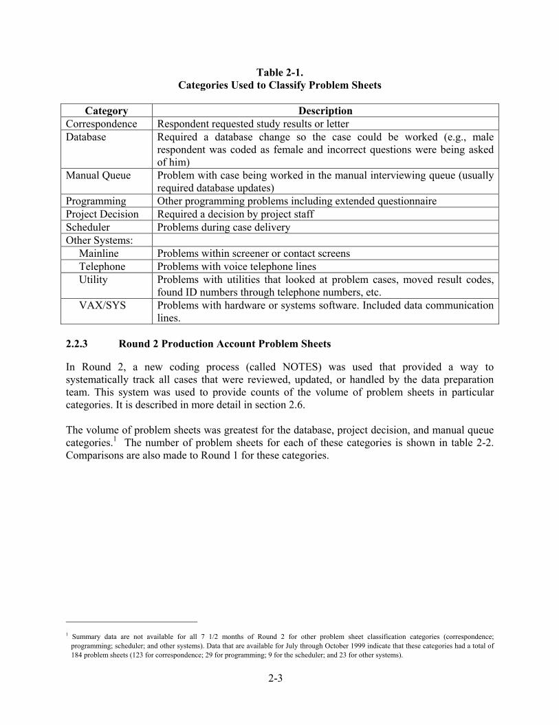
2.2 Problem Cases In the 1999 NSAF, 147,623 telephone households were screened and extended interviews were conducted in 44,499 households with 48,679 persons. Given the large number of interviews, several systems were in place to handle problem cases. One of the main tasks of the data editing staff was to handle interim cases with problems. In this section, the method that interviewers used to communicate problems is described, along with the system used by data editing staff to categorize them and a summary of the process for problem resolution. Also included is a description of a new coding process in Round 2 that provided a way to systematically track all cases that were reviewed, updated, or handled by the data preparation team. A comparison of problem cases in Rounds 1 and 2 is also provided. 2.2.1 Communication of Problems During data collection, an interviewer who experienced a problem while working a case could alert the project team in one of two ways. One method was to fill out a problem sheet on the case. Problem sheets from all the telephone facilities were sent to a staff member at the Westat Telephone Research Center (TRC) who distributed them to the appropriate Westat department or project staff person. The other method of communicating problems was to assign a problem result code to the case, without completing a paper problem sheet. These cases were then reviewed electronically by a TRC supervisor and either refielded to the interviewers or distributed to telephone center, programming, or project staff as appropriate. 2.2.2 Classification of Problem Sheets The classification system for problem sheets was the same as that used in Round 1. The categories described in table 2-1 are used by the TRC for most large telephone survey projects, with the exception of “Manual Queue,” which is specific to NSAF (see 1999 NSAF Telephone Survey Methods, Report No. 6, in the NSAF Methodology Series for a detailed discussion of the manual queue activities). Problems were grouped into seven categories.

2-3

Table 2-1. Categories Used to Classify Problem Sheets

Category Description

Correspondence Respondent requested study results or letter Database Required a database change so the case could be worked (e.g., male

respondent was coded as female and incorrect questions were being asked of him)

Manual Queue Problem with case being worked in the manual interviewing queue (usually required database updates)

Programming Other programming problems including extended questionnaire Project Decision Required a decision by project staff Scheduler Problems during case delivery Other Systems: Mainline Problems within screener or contact screens Telephone Problems with voice telephone lines Utility Problems with utilities that looked at problem cases, moved result codes,

found ID numbers through telephone numbers, etc. VAX/SYS Problems with hardware or systems software. Included data communication

lines. 2.2.3 Round 2 Production Account Problem Sheets In Round 2, a new coding process (called NOTES) was used that provided a way to systematically track all cases that were reviewed, updated, or handled by the data preparation team. This system was used to provide counts of the volume of problem sheets in particular categories. It is described in more detail in section 2.6. The volume of problem sheets was greatest for the database, project decision, and manual queue categories.1 The number of problem sheets for each of these categories is shown in table 2-2. Comparisons are also made to Round 1 for these categories.

1 Summary data are not available for all 7 1/2 months of Round 2 for other problem sheet classification categories (correspondence;

programming; scheduler; and other systems). Data that are available for July through October 1999 indicate that these categories had a total of 184 problem sheets (123 for correspondence; 29 for programming; 9 for the scheduler; and 23 for other systems).

2-4

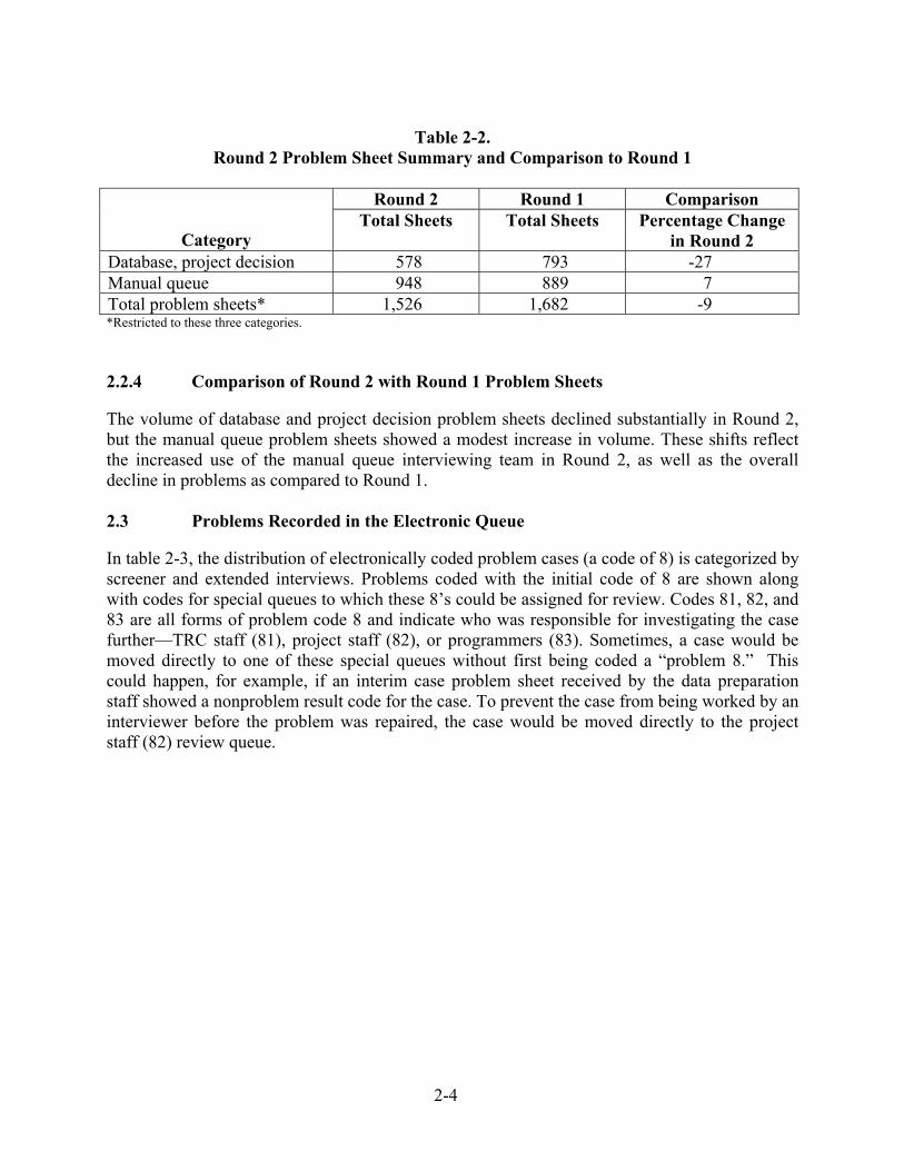
Table 2-2.

Round 2 Problem Sheet Summary and Comparison to Round 1

Round 2 Round 1 Comparison

Category Total Sheets Total Sheets Percentage Change

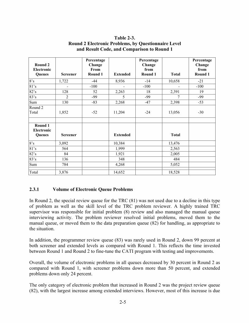
in Round 2 Database, project decision 578 793 -27 Manual queue 948 889 7 Total problem sheets* 1,526 1,682 -9 *Restricted to these three categories. 2.2.4 Comparison of Round 2 with Round 1 Problem Sheets The volume of database and project decision problem sheets declined substantially in Round 2, but the manual queue problem sheets showed a modest increase in volume. These shifts reflect the increased use of the manual queue interviewing team in Round 2, as well as the overall decline in problems as compared to Round 1. 2.3 Problems Recorded in the Electronic Queue In table 2-3, the distribution of electronically coded problem cases (a code of 8) is categorized by screener and extended interviews. Problems coded with the initial code of 8 are shown along with codes for special queues to which these 8’s could be assigned for review. Codes 81, 82, and 83 are all forms of problem code 8 and indicate who was responsible for investigating the case further—TRC staff (81), project staff (82), or programmers (83). Sometimes, a case would be moved directly to one of these special queues without first being coded a “problem 8.” This could happen, for example, if an interim case problem sheet received by the data preparation staff showed a nonproblem result code for the case. To prevent the case from being worked by an interviewer before the problem was repaired, the case would be moved directly to the project staff (82) review queue.

2-5

Table 2-3.

Round 2 Electronic Problems, by Questionnaire Level and Result Code, and Comparison to Round 1

Round 2 Electronic

Queues

Screener

Percentage Change From

Round 1

Extended

Percentage Change

from Round 1

Total

Percentage Change

from Round 1

8’s 1,722 -44 8,936 -14 10,658 -21 81’s - -100 - -100 - -100 82’s 128 52 2,263 18 2,391 19 83’s 2 -99 5 -99 7 -99 Sum 130 -83 2,268 -47 2,398 -53 Round 2 Total

1,852

-52

11,204

-24

13,056

-30

Round 1

Electronic Queues

Screener

Extended

Total

8’s 3,092 10,384 13,476 81’s 564 1,999 2,563 82’s 84 1,921 2,005 83’s 136 348 484 Sum 784 4,268 5,052

Total 3,876 14,652 18,528 2.3.1 Volume of Electronic Queue Problems In Round 2, the special review queue for the TRC (81) was not used due to a decline in this type of problem as well as the skill level of the TRC problem reviewer. A highly trained TRC supervisor was responsible for initial problem (8) review and also managed the manual queue interviewing activity. The problem reviewer resolved initial problems, moved them to the manual queue, or moved them to the data preparation queue (82) for handling, as appropriate to the situation. In addition, the programmer review queue (83) was rarely used in Round 2, down 99 percent at both screener and extended levels as compared with Round 1. This reflects the time invested between Round 1 and Round 2 to fine-tune the CATI program with testing and improvements. Overall, the volume of electronic problems in all queues decreased by 30 percent in Round 2 as compared with Round 1, with screener problems down more than 50 percent, and extended problems down only 24 percent. The only category of electronic problem that increased in Round 2 was the project review queue (82), with the largest increase among extended interviews. However, most of this increase is due

2-6

to the movement of a group of several hundred manual queue problem 8’s to the 82 queue in July. This type of result code shift was unique to Round 2 and was performed by the data preparation staff to alleviate a backlog of problems that had accumulated during two preliminary sample closeouts in June and July. The data preparation staff checked the project review queue daily, and problems were resolved using procedures developed during Round 1. Section 2.6 on NOTES contains descriptions and frequencies of the types of problems resolved through the project review queue. 2.3.2 Comparison of Round 2 with Round 1 Electronic Problems, Discussion of

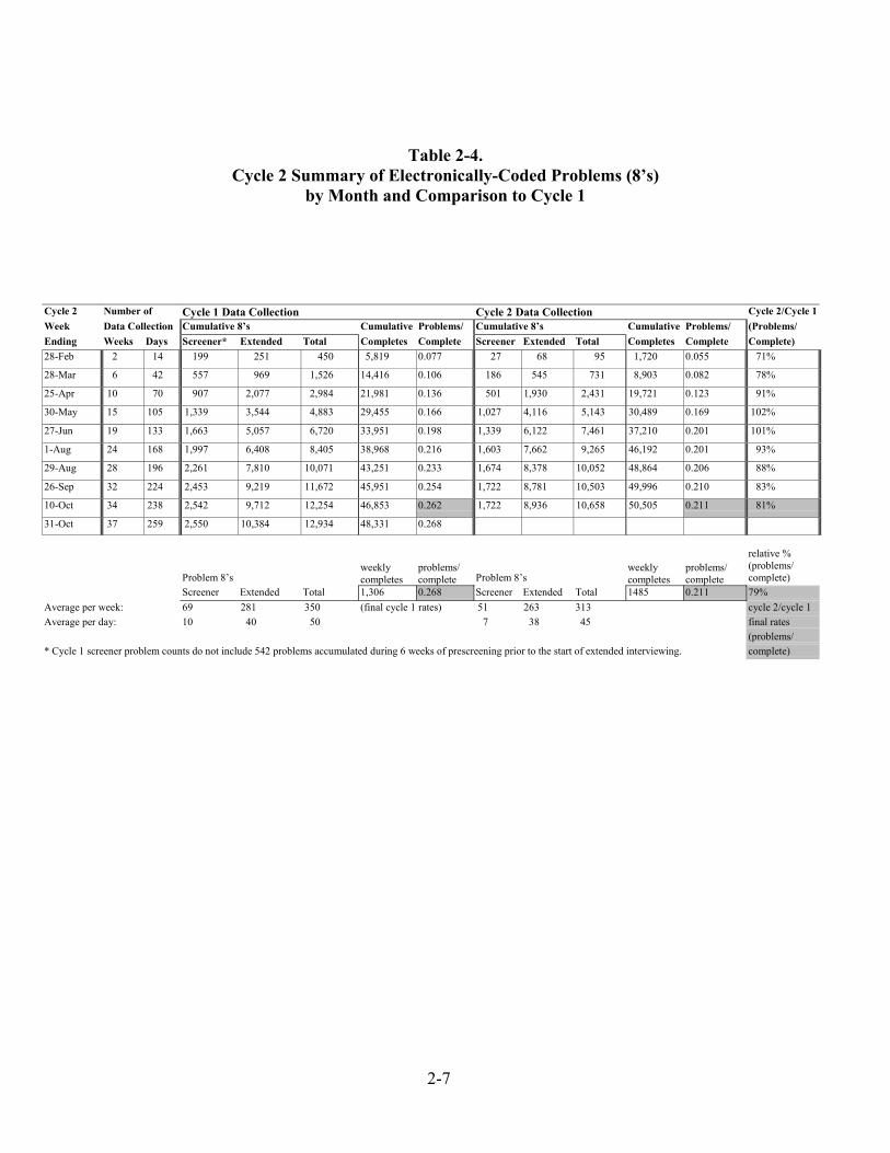
Volume over Time Table 2-4 compares the accumulation of problem 8’s during both rounds of data collection and contains a ratio of “problems per complete,” calculated as cumulative problems divided by cumulative completes, at different stages of data collection. As many things were different in Round 2, including a higher goal of extended interviews and different screening procedures, this ratio was a way to make a fair comparison between rounds. The problems per complete ratio for Round 2 was divided by the ratio for Round 1 to achieve a “relative percent” status of Round 2 problems, shown in the far right column of table 2-4. The Round 2 problem “relative percent” was used by the data preparation staff as a measure to gauge performance, and when the value approached “1” extra efforts were made to reduce additional problem accumulation. Round 2 problems show a sharp increase during the first four months of data collection, after which the volume plateaus and then declines, relative to Round 1. There are several reasons for this movement in the “relative percent” column in table 2-4. The manual queue interviewing activity started almost two months earlier in Round 2 than in Round 1, and cases in this queue tend to return to a problem status more often than other cases. In addition, during Round 2 there were two early sample closeouts, one at the beginning of June, and another at the beginning of July. A surge of problems is common during sample closeouts, and the combination of this activity with the early opening of the manual queue led to a 102 percent relative percent by the end of May, which declined only to 101 percent by the end of June. However, the implementation of Round 2 “partial complete” rules, starting in July, began to remove some cases from the workflow that otherwise may have become problems. These rules allowed cases that had completed only a portion of the extended interview (through section D), but had received a sufficient number of call attempts, to be considered final partial completes. In addition, an improved CATI program led to fewer overall problems due to common preventable errors throughout the course of data collection. The final Round 2 relative percentage of 79 percent is evidence of the marked decline in problems during this round of data collection. Table 2-4 also shows average numbers of problem 8’s per day and per week, by questionnaire level and overall, for both Round 2 and Round 1.

2-7

Table 2-4. Cycle 2 Summary of Electronically-Coded Problems (8’s)

by Month and Comparison to Cycle 1

Cycle 2 Number of Cycle 1 Data Collection Cycle 2 Data Collection Cycle 2/Cycle 1Week Data Collection Cumulative 8’s Cumulative Problems/ Cumulative 8’s Cumulative Problems/ (Problems/Ending Weeks Days Screener* Extended Total Completes Complete Screener Extended Total Completes Complete Complete)28-Feb 2 14 199 251 450 5,819 0.077 27 68 95 1,720 0.055 71%

28-Mar 6 42 557 969 1,526 14,416 0.106 186 545 731 8,903 0.082 78%

25-Apr 10 70 907 2,077 2,984 21,981 0.136 501 1,930 2,431 19,721 0.123 91%

30-May 15 105 1,339 3,544 4,883 29,455 0.166 1,027 4,116 5,143 30,489 0.169 102%

27-Jun 19 133 1,663 5,057 6,720 33,951 0.198 1,339 6,122 7,461 37,210 0.201 101%

1-Aug 24 168 1,997 6,408 8,405 38,968 0.216 1,603 7,662 9,265 46,192 0.201 93%

29-Aug 28 196 2,261 7,810 10,071 43,251 0.233 1,674 8,378 10,052 48,864 0.206 88%

26-Sep 32 224 2,453 9,219 11,672 45,951 0.254 1,722 8,781 10,503 49,996 0.210 83%

10-Oct 34 238 2,542 9,712 12,254 46,853 0.262 1,722 8,936 10,658 50,505 0.211 81%

31-Oct 37 259 2,550 10,384 12,934 48,331 0.268

Problem 8’sweeklycompletes

problems/complete Problem 8’s

weeklycompletes

problems/complete

relative %(problems/complete)

Screener Extended Total 1,306 0.268 Screener Extended Total 1485 0.211 79%Average per week: 69 281 350 (final cycle 1 rates) 51 263 313 cycle 2/cycle 1Average per day: 10 40 50 7 38 45 final rates

(problems/* Cycle 1 screener problem counts do not include 542 problems accumulated during 6 weeks of prescreening prior to the start of extended interviewing. complete)

2-8

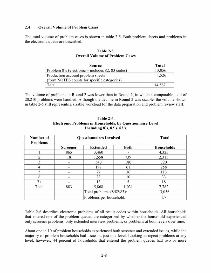
2.4 Overall Volume of Problem Cases The total volume of problem cases is shown in table 2-5. Both problem sheets and problems in the electronic queue are described.

Table 2-5. Overall Volume of Problem Cases

Source Total

Problem 8’s (electronic – includes 82, 83 codes) 13,056 Production account problem sheets (from NOTES counts for specific categories)

1,526

Total 14,582 The volume of problems in Round 2 was lower than in Round 1, in which a comparable total of 20,210 problems were handled. Although the decline in Round 2 was sizable, the volume shown in table 2-5 still represents a sizable workload for the data preparation and problem review staff.

Table 2-6. Electronic Problems in Households, by Questionnaire Level

Including 8’s, 82’s, 83’s

Number of Problems

Questionnaires Involved Total

Screener Extended Both Households 1 865 3,460 - 4,325 2 18 1,558 739 2,315 3 - 540 180 720 4 - 197 61 258 5 - 77 36 113 6 - 23 10 33

7+ - 13 5 18 Total 883 5,868 1,031 7,782

Total problems (8/82/83): 13,056 Problems per household: 1.7 Table 2-6 describes electronic problems of all result codes within households. All households that entered one of the problem queues are categorized by whether the household experienced only screener problems, only extended interview problems, or problems at both levels over time. About one in 10 of problem households experienced both screener and extended issues, while the majority of problem households had issues at just one level. Looking at repeat problems at any level, however, 44 percent of households that entered the problem queues had two or more

2-9

problems over the course of data collection. This could have been just an 8 followed by an 82, or it could be multiple, discrete problem instances over the course of the case’s history. 2.5 Problem Resolutions

Rules for handling problem cases were developed during Round 1 of the study and were used again in Round 2. Having these procedures in place allowed for a timely resolution of cases with reported problems. For some problems, no database updates were necessary and the cases were simply released for general interviewing with a message. For example, if a case was stopped in the middle of the health insurance section of the extended interview, and the problem message typed by the interviewer read, “respondent remembered that their health insurance is a private plan, and not from their employer—can’t back up to change the answer,” the solution to this was to release the case with a message stating, “case will restart in Section E and re-ask the insurance questions.” Similarly, problems related to miscoding responses in the screener questionnaire generally did not require database updates, because every time the screener was reopened it restarted at the beginning and re-asked every question. As long as the screener was assigned a problem result code while still an interim—not completed—screener, the database would be reset when the questionnaire was reopened. In general, only the cases moved by the TRC into the special review queues were investigated for possible updates. When cases were changed, they were often re-released for general interviewing. Some examples of the types of cases reviewed by project staff were those in which an error was made in enumerating a household member or when the person named as most knowledgeable (the MKA) about the child had to be changed. Other types of problems required special interviewer handling, even after changes such as MKA updates were made to the database. Some problems required special handling without database changes, such as cases where the respondent for the extended interview had moved or the respondent was a student living away at school. These problems were moved to the manual queue. The manual queue interviewers served, in a sense, as an auxiliary branch of the data editing team. They were trained to recognize a wide variety of problem situations, many involving enumeration errors, and to proceed slowly to avoid repeating the error. They were also given the authority to offer small monetary incentives to gain cooperation from proxies or facilitators when the selected respondent was unable to complete the interview. The following six primary methods of quality control were used in the study: limiting the number of staff who made updates; using flowcharts to understand complex sections of the questionnaire; using the CATI program to ensure edited cases conform to specifications; monthly data deliveries to identify and resolve systematic problems before the end of data collection; investigating issues found in programmatic data checks; and resolving roster updates interactively with the Urban Institute.

2-10

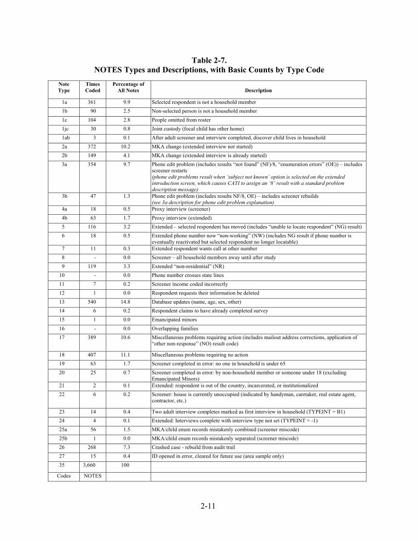
In addition, NOTES were coded for each case reviewed and updated by the data preparation staff, and the NOTES data were delivered to the Urban Institute in order to provide documentation of the purpose of all updates performed in Round 2. 2.6 Addition of NOTES Coding and Description of Results The NOTES feature added in Round 2 was motivated by the inability after Round 1 to report frequencies for the types of project review problems encountered during data collection. At the end of Round 1 a copy of all update records for updates performed by Westat was delivered to the Urban Institute as part of each case’s history. However, these records by themselves could not explain why a case was updated but could merely note that an update had been made. To alleviate these shortcomings in data preparation record keeping and reporting capabilities, the NOTES system was devised for Round 2. 2.6.1 NOTES Types and Basic Counts Table 2-7 contains all of the NOTES types used during Round 2, with counts and percents shown for each NOTES type.

2-11

Table 2-7.

NOTES Types and Descriptions, with Basic Counts by Type Code

Note Type

Times Coded

Percentage of All Notes

Description

1a 361 9.9 Selected respondent is not a household member 1b 90 2.5 Non-selected person is not a household member 1c 104 2.8 People omitted from roster 1jc 30 0.8 Joint custody (focal child has other home) 1ab 3 0.1 After adult screener and interview completed, discover child lives in household 2a 372 10.2 MKA change (extended interview not started) 2b 149 4.1 MKA change (extended interview is already started) 3a 354 9.7 Phone edit problem (includes results “not found” (NF)/8, “enumeration errors” (OE)) – includes

screener restarts (phone edit problems result when ‘subject not known’ option is selected on the extended introduction screen, which causes CATI to assign an ‘8’ result with a standard problem description message)

3b 47 1.3 Phone edit problem (includes results NF/8, OE) – includes screener rebuilds (see 3a description for phone edit problem explanation)

4a 18 0.5 Proxy interview (screener) 4b 63 1.7 Proxy interview (extended) 5 116 3.2 Extended – selected respondent has moved (includes “unable to locate respondent” (NG) result) 6 18 0.5 Extended phone number now “non-working” (NW) (includes NG result if phone number is

eventually reactivated but selected respondent no longer locatable) 7 11 0.3 Extended respondent wants call at other number 8 - 0.0 Screener – all household members away until after study 9 119 3.3 Extended “non-residential” (NR)

10 - 0.0 Phone number crosses state lines 11 7 0.2 Screener income coded incorrectly 12 1 0.0 Respondent requests their information be deleted 13 540 14.8 Database updates (name, age, sex, other) 14 6 0.2 Respondent claims to have already completed survey 15 1 0.0 Emancipated minors 16 - 0.0 Overlapping families 17 389 10.6 Miscellaneous problems requiring action (includes mailout address corrections, application of

“other non-response” (NO) result code)

18 407 11.1 Miscellaneous problems requiring no action 19 63 1.7 Screener completed in error: no one in household is under 65 20 25 0.7 Screener completed in error: by non-household member or someone under 18 (excluding

Emancipated Minors) 21 2 0.1 Extended: respondent is out of the country, incarcerated, or institutionalized 22 6 0.2 Screener: house is currently unoccupied (indicated by handyman, caretaker, real estate agent,

contractor, etc.)

23 14 0.4 Two adult interview completes marked as first interview in household (TYPEINT = B1) 24 4 0.1 Extended: Interviews complete with interview type not set (TYPEINT = -1) 25a 56 1.5 MKA/child enum records mistakenly combined (screener miscode) 25b 1 0.0 MKA/child enum records mistakenly separated (screener miscode) 26 268 7.3 Crashed case - rebuild from audit trail 27 15 0.4 ID opened in error, cleared for future use (area sample only) 35 3,660 100

Codes NOTES

2-12

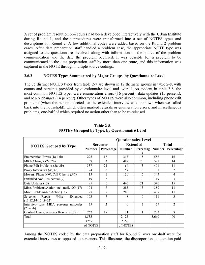
A set of problem resolution procedures had been developed interactively with the Urban Institute during Round 1, and these procedures were transformed into a set of NOTES types and descriptions for Round 2. A few additional codes were added based on the Round 2 problem cases. After data preparation staff handled a problem case, the appropriate NOTE type was assigned to the questionnaire involved, along with information on the source of the problem communication and the date the problem occurred. It was possible for a problem to be communicated to the data preparation staff by more than one route, and this information was captured in the NOTE through multiple source codings. 2.6.2 NOTES Types Summarized by Major Groups, by Questionnaire Level The 35 distinct NOTES types from table 2-7 are shown in 12 thematic groups in table 2-8, with counts and percents provided by questionnaire level and overall. As evident in table 2-8, the most common NOTES types were enumeration errors (16 percent), data updates (15 percent), and MKA changes (14 percent). Other types of NOTES were also common, including phone edit problems (when the person selected for the extended interview was unknown when we called back into the household), which often masked refusals or enumeration errors, and miscellaneous problems, one-half of which required no action other than to be re-released.

Table 2-8. NOTES Grouped by Type, by Questionnaire Level

Questionnaire Level

Screener Extended Total NOTES Grouped by Type Number Percentage Number Percentag

e Number Percentage

Enumeration Errors (1a-1ab) 275 18 313 15 588 16 MKA Changes (2a, 2b) 39 3 482 23 521 14 Phone Edit Problems (3a, 3b) 337 22 64 3 401 11 Proxy Interviews (4a, 4b) 24 2 57 3 81 2 Movers, Phone NW, Call Other # (5-7) 15 1 130 6 145 4 Extended Non-Residential (9) 119 8 - 0 119 3 Data Updates (13) 95 6 445 21 540 15 Misc. Problems/Action-incl. mail, NO (17) 104 7 285 13 389 11 Misc. Problems/No Action (18) 127 8 280 13 407 11 Screener Repair /Misc. Extended (11,12,14-16,19-22)

103 7 8 0 111 3

Interview type, MKA Screener miscodes (23-25b)

35 2 40 2 75 2

Crashed Cases, Screener Resets (26,27) 262 17 21 1 283 8 Total 1,535 2,125 3,660 100 42% 58% of NOTES of NOTES Among the NOTES coded by the data preparation staff for Round 2, over one-half were for extended interviews as opposed to screeners. This illustrates the disproportionate attention paid

2-13

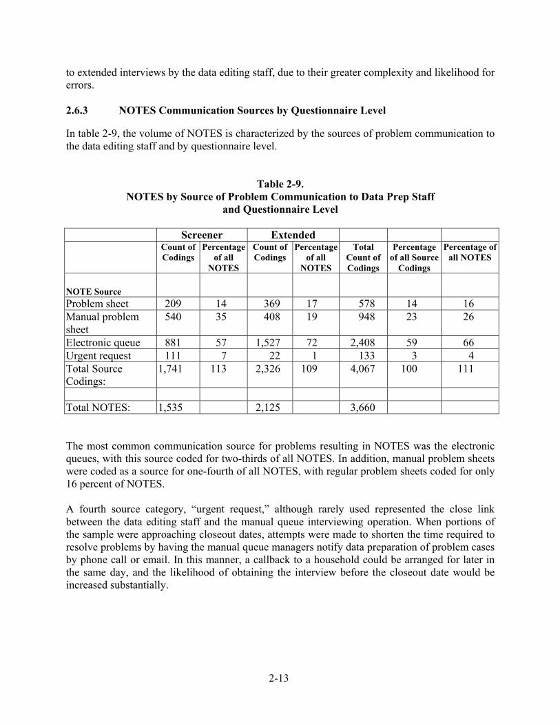
to extended interviews by the data editing staff, due to their greater complexity and likelihood for errors. 2.6.3 NOTES Communication Sources by Questionnaire Level In table 2-9, the volume of NOTES is characterized by the sources of problem communication to the data editing staff and by questionnaire level.

Table 2-9. NOTES by Source of Problem Communication to Data Prep Staff

and Questionnaire Level

Screener Extended Count of

Codings Percentage

of all NOTES

Count of Codings

Percentage of all

NOTES

Total Count of Codings

Percentage of all Source

Codings

Percentage of all NOTES

NOTE Source

Problem sheet 209 14 369 17 578 14 16 Manual problem sheet

540 35 408 19 948 23 26

Electronic queue 881 57 1,527 72 2,408 59 66 Urgent request 111 7 22 1 133 3 4 Total Source Codings:

1,741 113 2,326 109 4,067 100 111

Total NOTES: 1,535 2,125 3,660 The most common communication source for problems resulting in NOTES was the electronic queues, with this source coded for two-thirds of all NOTES. In addition, manual problem sheets were coded as a source for one-fourth of all NOTES, with regular problem sheets coded for only 16 percent of NOTES. A fourth source category, “urgent request,” although rarely used represented the close link between the data editing staff and the manual queue interviewing operation. When portions of the sample were approaching closeout dates, attempts were made to shorten the time required to resolve problems by having the manual queue managers notify data preparation of problem cases by phone call or email. In this manner, a callback to a household could be arranged for later in the same day, and the likelihood of obtaining the interview before the closeout date would be increased substantially.

2-14

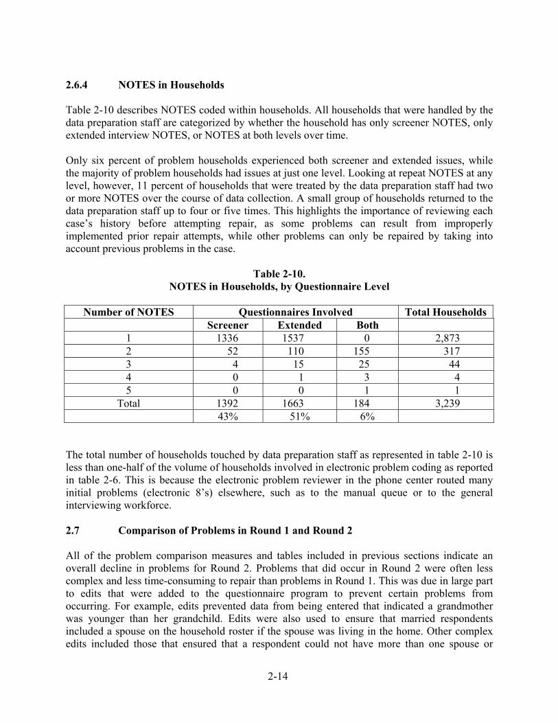
2.6.4 NOTES in Households Table 2-10 describes NOTES coded within households. All households that were handled by the data preparation staff are categorized by whether the household has only screener NOTES, only extended interview NOTES, or NOTES at both levels over time. Only six percent of problem households experienced both screener and extended issues, while the majority of problem households had issues at just one level. Looking at repeat NOTES at any level, however, 11 percent of households that were treated by the data preparation staff had two or more NOTES over the course of data collection. A small group of households returned to the data preparation staff up to four or five times. This highlights the importance of reviewing each case’s history before attempting repair, as some problems can result from improperly implemented prior repair attempts, while other problems can only be repaired by taking into account previous problems in the case.

Table 2-10. NOTES in Households, by Questionnaire Level

Number of NOTES Questionnaires Involved Total Households

Screener Extended Both 1 1336 1537 0 2,873 2 52 110 155 317 3 4 15 25 44 4 0 1 3 4 5 0 0 1 1

Total 1392 1663 184 3,239 43% 51% 6% The total number of households touched by data preparation staff as represented in table 2-10 is less than one-half of the volume of households involved in electronic problem coding as reported in table 2-6. This is because the electronic problem reviewer in the phone center routed many initial problems (electronic 8’s) elsewhere, such as to the manual queue or to the general interviewing workforce. 2.7 Comparison of Problems in Round 1 and Round 2 All of the problem comparison measures and tables included in previous sections indicate an overall decline in problems for Round 2. Problems that did occur in Round 2 were often less complex and less time-consuming to repair than problems in Round 1. This was due in large part to edits that were added to the questionnaire program to prevent certain problems from occurring. For example, edits prevented data from being entered that indicated a grandmother was younger than her grandchild. Edits were also used to ensure that married respondents included a spouse on the household roster if the spouse was living in the home. Other complex edits included those that ensured that a respondent could not have more than one spouse or

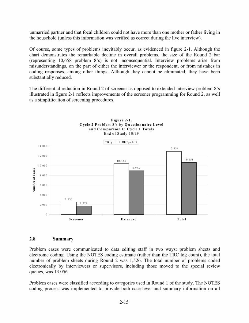
2-15

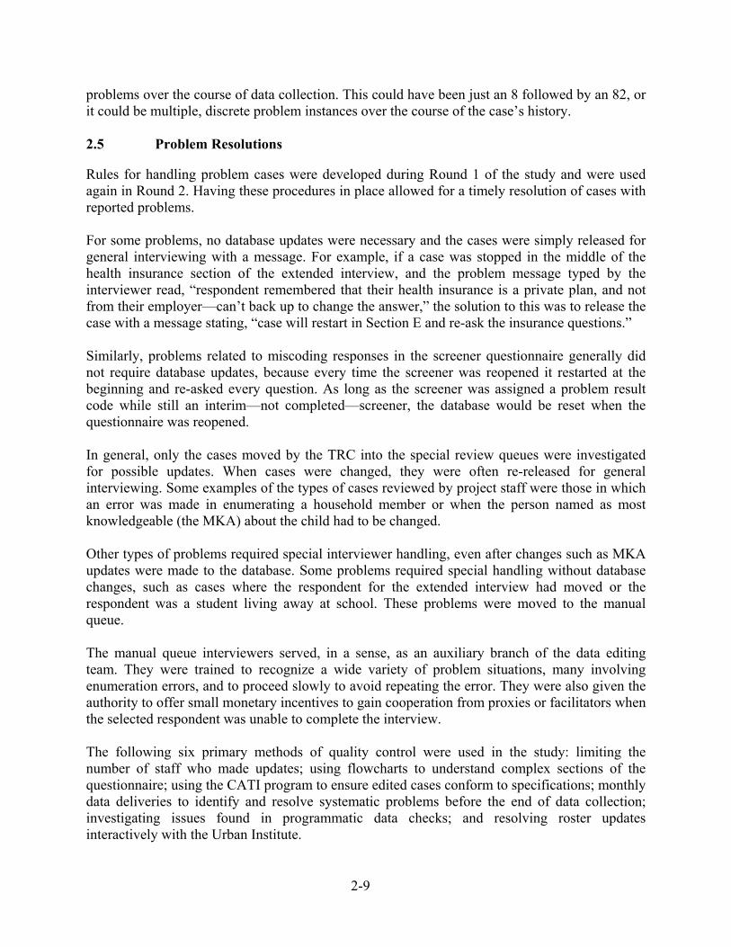
unmarried partner and that focal children could not have more than one mother or father living in the household (unless this information was verified as correct during the live interview). Of course, some types of problems inevitably occur, as evidenced in figure 2-1. Although the chart demonstrates the remarkable decline in overall problems, the size of the Round 2 bar (representing 10,658 problem 8’s) is not inconsequential. Interview problems arise from misunderstandings, on the part of either the interviewer or the respondent, or from mistakes in coding responses, among other things. Although they cannot be eliminated, they have been substantially reduced. The differential reduction in Round 2 of screener as opposed to extended interview problem 8’s illustrated in figure 2-1 reflects improvements of the screener programming for Round 2, as well as a simplification of screening procedures.

2.8 Summary Problem cases were communicated to data editing staff in two ways: problem sheets and electronic coding. Using the NOTES coding estimate (rather than the TRC log count), the total number of problem sheets during Round 2 was 1,526. The total number of problems coded electronically by interviewers or supervisors, including those moved to the special review queues, was 13,056. Problem cases were classified according to categories used in Round 1 of the study. The NOTES coding process was implemented to provide both case-level and summary information on all

F igure 2-1 .C ycle 2 P roblem 8 's by Q uestionnaire L evel

and C om parison to C ycle 1 T ota lsE nd of S tudy 10/99

2,550

10,384

12,934

1,722

8,936

10,658

0

2,000

4,000

6,000

8,000

10,000

12,000

14,000

Screener E xtended T otal

Num

ber

of C

ases

C ycle 1 C ycle 2

2-16

cases reviewed and repaired by the Westat data editing staff. Some of the corrections required individualized handling by specially trained interviewers. The problems in Round 2 were less time consuming and complex than they were in Round 1. Part of this was because procedures had already been developed during the previous round of the study. In addition, edits in CATI prevented many problems from occurring. 2.9 Comments Another important data editing task was reading and using interviewer comments. Comments are text phrases that interviewers type in special entry windows in computer-assisted telephone interviewing (CATI) when the respondent makes a statement that the interviewer wants to record but are unable to enter as a standard response in the questionnaire. Sometimes these phrases are merely an elaboration on a previously recorded response or an expression of opinion. Other times, they indicate that an update needs to be made. The purpose of comment review was in Round 2 was different from that in Round 1. In Round 1, all comments from specific sections of the questionnaire were reviewed for potential database updates, which were implemented by the Westat data editing staff. In Round 2, the Urban Institute decided prior to the start of data collection that systematic updates from comments would not be performed. Rather, comments were reviewed thoroughly at the beginning of data collection. Later, a sample of the comments was reviewed. This review had two goals: to identify any systematic CATI problems and repair the program and to locate interviewer training weaknesses and issue directives to the field on specific training issues. Some comments were used when making updates to completed cases identified through other means, such as problem sheets on completed interviews and programmatic checks run by the Urban Institute. If comments were present when interim problem cases were reviewed, these were taken into account by the data editing staff. 2.9.1 Comment Review During data collection, a list of comments was generated periodically for all completed interview households that had generated at least one comment. Comment review was performed on a “date completed” basis–that is, new lists of comments were generated starting with the date after the last comment list was produced for review. Interviewing for the NSAF was conducted at seven different interviewing facilities (three in Maryland and the others in Pennsylvania, New Jersey, Ohio, and Florida) that started data collection at different points. Comments from all sections of the questionnaire were read during the first two weeks of data collection at each facility. This was done in order to determine whether there were any major problems. After this, 10 percent of comments were read. 2.9.2 Use of Comments from Completes to Reinforce Training Issues During production the data editing staff notified the project team about any sections or questions of the questionnaire that were generating a larger number of comments than usual. Interviewer comments in Round 2 did not indicate any problems with questions, but they did point out areas

2-17

in which interviewers needed to have some training points reinforced. Interviewer memos were written to do this. For example, one section that received many comments was Section J. In Section J, respondents were asked about non-salary forms of income, including such things as annuities, pensions, interest, dividends, and rental property income. Once a form of income was indicated, a question was asked about whom received the income source. In some cases, respondents would say that no one had received a particular type of income and that they had answered an earlier question incorrectly. Interviewers entered comments to explain this situation. This was unnecessary, though, because there was a feature in Section J that allowed an interviewer to show that an income type had not been received. Interviewers were reminded of this from training in an interviewer memo. A similar issue arose in Section G. In Section G, respondents were asked about various forms of childcare. Once a childcare type was identified, a follow-up question was asked about hours in care. Occasionally, a type of care was misreported and not used. There was an option in the follow-up question to handle this situation. Interviewers were reminded to use this option rather than enter the information into comments. Another example of an issue brought to the attention of project staff from comments was the need to reinforce rounding rules. Interviewers recorded verbatim answers that did not fit answer categories in comments rather than rounding the answer to fit into an existing category. Interviewers were reminded of the rounding rules in a memo. 2.9.3 Summary Interviewer comments were useful for making updates to data in some sections of the questionnaire. However, not all sections of the questionnaire were eligible for updates because of their complexity. Lists of comments were periodically reviewed for potential CATI program or interviewer training problems. All comments were read during the first two weeks of data collection at each of the seven data collection sites. This was done in order to determine whether there were any major problems. After this, 10 percent of comments were read. Comments were not routinely reviewed for updates but did help resolve problem cases identified through other means. Some types of comments were used to give feedback to interviewers about ways to enter data during the interview. In general, the procedure in Round 2 was for Westat to update interim cases and make recommendations for updates to completed cases. The Urban Institute made the final decision about which updates to make and implemented the updates for completed cases. 2.10 Coding Coding for the 1999 NSAF was mostly conducted by the Urban Institute. This included coding for other-specify and open-ended questions. Other-specify questions were those in which a

2-18

question had some specific answer categories but also allowed for text to be typed into an “other” category. Open-ended questions had no precoded answer categories. Coding was also done for three questions about occupation and industry in the questionnaire. The first asked about the kind of industry the person worked in for his or her main job. Another question asked whether the business or organization was mainly manufacturing or something else. A third question asked what kind of work the person did, that is, what was his or her occupation. Because the codes for the occupation and industry questions needed to be consistent with coding conducted by the U.S. Census Bureau, Westat sent several groups of cases as they were completed to Census for coding. Census returned the codes, which Westat then posted to the database. 2.11 Quality Control Quality control was maintained in several ways. Six of the primary methods used to ensure accurate data editing are discussed here. 2.11.1 Limiting the Number of Staff Who Made Updates In order to avoid contaminating the data, Westat limited the number of people making updates to the database. Updates were made only by the two-person data editing staff who were very familiar with the questionnaire and had been trained specifically for the NSAF. 2.11.2 Using Flowcharts In Round 1, the data editing staff created flowcharts of the CATI specifications for the sections that were eligible for comment review. These flowcharts assisted in knowing which edits would affect other sections of the questionnaire. Although the questionnaire changed somewhat in Round 2, the flowcharts could still be used to indicate which questions would be affected by updates to the interview. Knowledge of the flowcharts assisted in making changes and in advising the Urban Institute about the effects of recommended edits to cases. 2.11.3 Using CATI Program to Ensure Clean Data For many types of case repairs performed by Westat, the CATI program was used to ensure that revised completed interviews conformed to specifications. For example, some errors located in completed interviews suggested a very large number of updates to individual cases. Rather than attempting to implement such large numbers of updates, the case would be re-opened and the data entered again, which ensured the new complete would not have errors related to updating. The same approach was used for errors involving the record structure of a completed interview, such as a mis-assignation of an MKA ID.

2-19

2.11.4 Monthly Data Deliveries Data for completed interviews were delivered every month so that the Urban Institute could identify problems in completes while data collection was still being performed. In this manner, any systematic problems could be identified and repaired before the end of the study. In addition, the Urban Institute was able to begin investigating other types of errors in completed interviews a few months after the start of data collection, which accelerated the error resolution process. 2.11.5 Programmatic Checks Westat investigated inconsistencies or illogical patterns found in a series of programmatic checks performed by the Urban Institute. These checks focused on roster-based errors in completed interviews, such as: A child has two mothers or two fathers living in the household, Unlikely or impossible age/relationship combinations, A respondent has multiple spouses or unmarried partners, Problems with MKA or Child IDs, and Duplicate persons in the roster.

The volume of such cases in Round 2 was much lower than in Round 1, due to improvements in the CATI program that checked for many types of errors at the time that interviews were conducted. The following types of errors found in Round 1 were all prevented from occurring without confirmation by the respondent by the Round 2 CATI program: Respondents with multiple spouses or unmarried partners in the household, Married respondents missing spouses (omitted in roster), Children with more than one mother or father in the household, Parents younger than their child, Biological parents less than 10 years older than their child, Grandparents less than 20 years older than their grandchild, and Great-grandparents less than 30 years older than their great-grandchild.

In Round 1, approximately 1,300 completed interview households with these types of errors were identified through programmatic checks, with most requiring repair. The Round 2 volume of case review for errors found through programmatic checks was approximately 10 percent of the Round 1 volume. The problems that were found in Round 2 stemmed from errors during the interview, such as misreporting or miscoding of relationships or ages, or from changes made by the data editing staff to interim cases, such as updating one, but not all, of the variables that were dependent on other variables in the interview. Recommendations were made by Westat for updating the interview and were evaluated by the Urban Institute for the final decision. If the source of the error was an incomplete or incorrect case repair originated by Westat, the Westat data editing staff corrected the error prior to the next data delivery. If the problem affected the record

2-20

structure of the case, Westat re-entered the data in order to generate the proper record structure prior to the next data delivery. The Urban Institute resolved other errors in completed interviews in the delivered files. 2.11.6 Interactive Resolution of Updates to Completed Interview Roster Data for

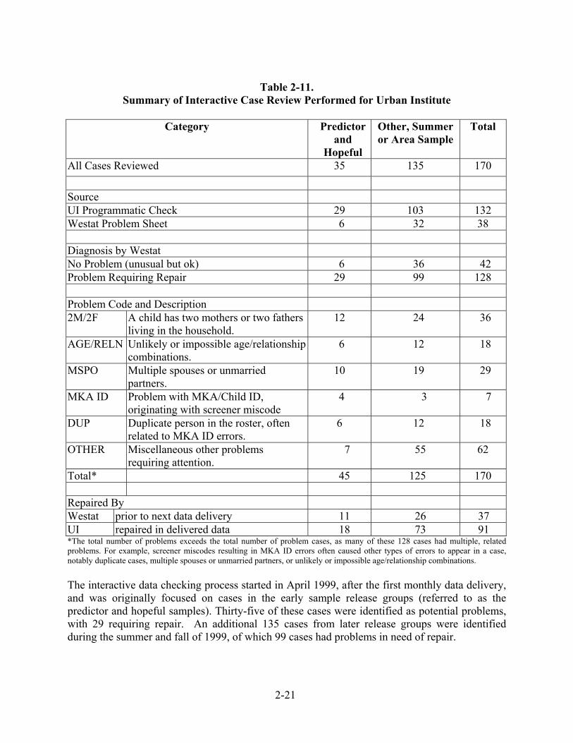
Consistency with Round 1 As in Round 1, Westat and the Urban Institute worked together to decide how to accomplish roster updates to completed interview data that were likely to result in “downstream effects” to cases. This interactive process was important to ensure that data editing was performed correctly and editing decisions were consistent with Round 1 procedures. The Urban Institute was responsible in Round 2 for performing most updates to completed interview data, whereas most updates to completed interviews in Round 1 were performed by Westat data editing staff. Once the Urban Institute identified a set of completed interview households with similar roster-based errors, Westat reviewed the cases and diagnosed problems, then recommended procedures for repair by either Westat or the Urban Institute. In some instances, Westat re-entered cases prior to the next data delivery in order to create the proper record structure for the Urban Institute. However, the Urban Institute performed the majority of roster repairs in the delivered data files. To ensure consistency between Round 2 and Round 1, the same Westat data manager that performed all such updates in Round 1 reviewed problem cases identified through programmatic checks in Round 2 and provided editing recommendations for each case to the Urban Institute. The Urban Institute then implemented these updates and resolved any downstream effects of the changes. A total of 132 cases were identified for review through Urban Institute checks, and an additional 38 cases were added from Westat problem sheets for completed interviews. Table 2-11 contains a summary of the 170 cases reviewed and the types of errors found.

2-21

Table 2-11.

Summary of Interactive Case Review Performed for Urban Institute

Category Predictor and

Hopeful

Other, Summer or Area Sample

Total

All Cases Reviewed 35 135 170 Source UI Programmatic Check 29 103 132 Westat Problem Sheet 6 32 38 Diagnosis by Westat No Problem (unusual but ok) 6 36 42 Problem Requiring Repair 29 99 128 Problem Code and Description 2M/2F A child has two mothers or two fathers

living in the household. 12 24 36

AGE/RELN Unlikely or impossible age/relationship combinations.

6 12 18

MSPO Multiple spouses or unmarried partners.

10 19 29

MKA ID Problem with MKA/Child ID, originating with screener miscode

4 3 7

DUP Duplicate person in the roster, often related to MKA ID errors.

6 12 18

OTHER Miscellaneous other problems requiring attention.

7 55 62

Total* 45 125 170 Repaired By Westat prior to next data delivery 11 26 37 UI repaired in delivered data 18 73 91 *The total number of problems exceeds the total number of problem cases, as many of these 128 cases had multiple, related problems. For example, screener miscodes resulting in MKA ID errors often caused other types of errors to appear in a case, notably duplicate cases, multiple spouses or unmarried partners, or unlikely or impossible age/relationship combinations. The interactive data checking process started in April 1999, after the first monthly data delivery, and was originally focused on cases in the early sample release groups (referred to as the predictor and hopeful samples). Thirty-five of these cases were identified as potential problems, with 29 requiring repair. An additional 135 cases from later release groups were identified during the summer and fall of 1999, of which 99 cases had problems in need of repair.

2-22

One-fourth of the 170 cases reviewed had unusual information, but did not contain errors. These include situations such as a child with both a biological father and a stepfather living in the household, biological mothers under the age of 16, and households with twins or other valid “duplicate” persons. The types of errors that were found were often related, so the total number of errors was 170 for a total of 128 problem cases. That is, a case would be identified through two programmatic checks as having two distinct types of errors, when in fact one of the errors was directly linked to the occurrence of the other error. Examples of multiple, related problems include the following situations. An error is made in recording the MKA ID, such that a duplicate MKA record is created

with the same name, leading to multiple mothers for the children, and multiple spouses for the father.

A child with the same first name as his father is accidentally coded as a spouse to his mother leading to an unlikely age/relationship combination for the boy and multiple spouses for the mother.

Due to the complexity of repairs affecting record structure, including the first example listed above, Westat re-entered cases with slight adjustments where errors had been made and redelivered the data in the next data delivery. Other types of repairs were much more straightforward, requiring simple relationship updates or other minor updates, and were performed on the data files at the Urban Institute. 2.12 Editing for Confidentiality Data made available for Public Use has been manipulated or edited to ensure the confidentiality of survey respondents. This type of editing included excluding variables and constructing new variables based on the original variables, top and/or bottom coding of values and data blurring. 2.12.1 Constructing New Variables New variables were constructed from several source variables and by collapsing values for a categorical variable. When survey questions identified relatively rare populations, a new variable was constructed, combining cases into one or more broad groups. For a single categorical variable, one or more values were combined. For example, in response to one of the questions on the NSAF survey, a respondent could either provide the exact year they came to live in the U.S., or they could report how many of years ago that they came to live in the U.S. Thus, there are two source variables were created, year of arrival and how many years ago did they arrive. Knowing, when a person came to the U.S. does pose a confidentiality issue, thus a public use variable was created that combines the two source variables into categories of 0-4 years ago, 5-9 years ago and more than 10 years ago. Family income is another variable that is constructed from several source variables, in which source variables are not released.

2-23

2.12.2 Top and Bottom Coding and Data Blurring Extreme and relatively rare cases that fall at the top or bottom of a distribution were recoded to lower of higher value. For example, any respondents over the age of 85 were coded as being 85. Questions that ask income amounts, child support amounts, AFDC/TANF payments, child care payments are all variables that have been top and bottom coded. The usual rule is to top code at 99th percentile value and bottom code at the 1st percentile value. This rule varied slightly depending upon the number of respondents or if there is a more natural value to choose as the bottom or top code. In addition to top and bottom coding many of the questions that ask for dollar amounts (income, child support, AFDC/TANF , child care) have been blurred in order to prevent inadvertent disclosure. To blur a variables data, the values for the variable is first sorted in descending order, and the average value is calculated for every ten records. This process protects the confidential information provided by the respondent, while preserving the overall statistical integrity of the data. For more information on blurring process see "Protection of Taxpayer Confidentiality with Respect to the Tax Model" (Strudler, Oh, and Scheuren 1986).

3-1

Chapter 3

Data Coding 3.1 Introduction to Data Coding and Review This chapter details data coding procedures completed during the course of Round 2. It begins with a discussion of the coding of the "other specify" variables. Compared to Round 1, Round 2 demonstrates considerable improvements in both the design of the coding procedures and the documentation of their execution. Section 3.1 explains the coding procedures in depth followed by a section 3.2 a short summary section. 3.1.1 Coding Other Specify Variables The other specify coding of Round 2 NSAF data was completed between May 1999 and May 2000. In the first round, Westat coded most of the “other specify” responses. Then Westat and the Urban Institute worked together to code problem cases. This process involved filling out problem sheets and assigning electronic problem result codes. (For an in-depth discussion of this process, refer to 1997 Methodology Report No. 10 on Data Editing and Imputation.)

In Round 1, many of the other specify variables were coded by hand, without a structured set of guidelines. Accordingly, even though quality control measures were implemented (see 1997 Methodology Report No. 10), there were some inconsistencies in the coding. In Round 2, a new coding process was employed to code the data more efficiently and consistently than the hand coding that was done in Round 1. This human-aided computer coding process featured two major components. First, with instructions developed by the coder and a computer program was written that put the responses into categories. Second, the categories assigned by the computer were checked and the coder reviewed in the data base the computer coded responses. 3.1.2 The Look-Up Table With the parameters specified by the coder, a computer program uses a set of mapping instructions to map actual responses to their appropriate categories. The coder forms these mapping instructions into what is called a look-up table. The look-up table is constructed in list form; on the left-hand side, a category is listed and to the right, a response-type appropriate to that category is listed. The next line will have another category followed by a response type that fits into that category. The coder forms this look-up table until most of the types of responses that appear in the raw data are included in the list. Figure 3-1 shows a few lines taken from the look-up table for the NSAF variable KAWORKD – “What is required to receive TANF or AFDC?”.

3-2

Figure 3-1.

Sample Lines from KAWORKD Look-up Table

1 LOOK FOR A JOB ATTEND A JOB SEARCH SCHOOL 1 LOOK FOR A JOB LOOK FOR JOB 1 LOOK FOR A JOB PROGRAM TO FIND JOB 1 LOOK FOR A JOB SEARCH FOR WORK 2 WORK IN A PAID JOB SELF EMPLOYMENT AT MIN WAGE 2 WORK IN A PAID JOB WORKING IN FAST-FOOD PLACE 3 WORK IN AN UNPAID JOB COMMUNITY SERVICE 3 WORK IN AN UNPAID JOB DO VOLUNTEER WORK 4 ATTEND SCHOOL OR TRAIN. ATTENDED SEMINARS 4 ATTEND SCHOOL OR TRAIN. GET GED 4 ATTEND SCHOOL OR TRAIN. GO TO A CLASS 4 ATTEND SCHOOL OR TRAIN. PARENTING CLASS 5 WORK-REALTED/MULT ACTIV REQ ATTEND JOB SERVICES 5 WORK-REALTED/MULT ACTIV REQ HAD TO WORK OR GO TO SCHOOL 5 WORK-REALTED/MULT ACTIV REQ JOBS PROGRAM 5 WORK-REALTED/MULT ACTIV REQ MUST ATTEND PROJECT MEETING 5 WORK-REALTED/MULT ACTIV REQ WORK PROGRAM 6 STAY HOME W/ CHILDREN MUST STAY HOME WITH KIDS 6 STAY HOME W/ CHILDREN TAKE CARE OF CHILDREN 7 KEEP CHILDREN IN SCHOOL CHILDREN CANT MISS SCHOOL 7 KEEP CHILDREN IN SCHOOL KIDS HAVE TO BE IN SCHOOL 3.1.3 Matching Misspelled or Grammatically Incorrect Data in Look-up For most of the Round 2 variables, the look-up table was created initially using codes and phrases from Round 1. The initial look-up table was then edited and reviewed for spelling and grammatical errors so that there is a standard for the spelling of words in the matching process. Sometimes the phrases in the raw data file are either spelled incorrectly or differently than the same words on the look-up table. LOOKUP makes allowances for these differences in two ways. 1) It employs a Soundex device to match words at level 3 (see description of match levels below). 2) It allows words and phrases in the raw data to be cleaned before LOOKUP searches for their matches in the look-up table. This cleaning process is done through the use of parameter file or PARMFILE. The parameter file contains all of the information about the filenames of the data files, parameters that can be changed in the matching process, and words and phrases that are to be changed before the matching of raw phrases to LOOKUP phrases. Raw phrases can be changed by the phrase or by the word. The coder may also decide to have some words deleted before the matching process. This process does not change the actual raw data, it just changes the phrases for the time that the program is being run. These “clean” phrases are then used by LOOKUP instead of the original phrases to search for matches in the table. If LOOKUP receives no instructions to change all or part of a phrase in the Parmfile, it uses the

3-3

original raw phrase to find a match on the table. A sample PARMFILE (Figure 3-2) is presented on the following page.

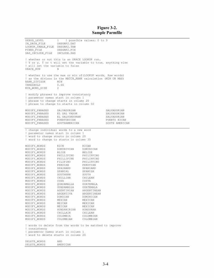
3-4

Figure 3-2. Sample Parmfile

DEBUG_LEVEL 1 ! possible values: 0 to 9 IN_DATA_FILE OHSGRP2.DAT LOOKUP_TABLE_FILE OHSGRP2.TAB FIXED_FILE OHSGRP2.FIX SAS_INCLUDE_FILE INCLUDE.SAS ! whether or not this is an ORACE LOOKUP run. ! Y or y, T or t will set the variable to true, anything else ! will set the variable to false ORACE_RUN N ! whether to use the max or min of(LOOKUP words, Raw words) ! as the divisor in the MATCH_RANK calculation (MIN OR MAX) RANK_DIVISOR MIN THRESHOLD 0.66 MIN_WORD_SIZE 2 ! modify phrases to improve consistancy ! parameter names start in column 1 ! phrase to change starts in column 20 ! phrase to change to starts in column 50 MODIFY_PHRASES SA;VADORIAN SALVADORIAN MODIFY_PHRASES EL SAL VADOR SALVADORIAN MODIFY_PHRASES EL SALVORDORAN SALVADORIAN MODIFY_PHRASES PUERTORICAN PUERTO RICAN MODIFY_PHRASES SOUTHAMERICAN SOUTH AMERICAN ! change individual words to a new word ! parameter names start in column 1 ! word to change starts in column 20 ! word to change to starts in column 35 MODIFY_WORDS RICN RICAN MODIFY_WORDS DOMINIVCAN DOMINICAN MODIFY_WORDS BLIZE BELIZE MODIFY_WORDS PHILLIPINO PHILIPPINO MODIFY_WORDS PHILLIPINE PHILIPPINO MODIFY_WORDS FILIPINO PHILIPPINO MODIFY_WORDS PERUIAN PERUVIAN MODIFY_WORDS SPAINARD SPANIARD MODIFY_WORDS SPANIAL SPANISH MODIFY_WORDS SOUTHERN SOUTH MODIFY_WORDS CHILLIAN CHILEAN MODIFY_WORDS COSA COSTA MODIFY_WORDS QUADAMALLA GUATEMALA MODIFY_WORDS GUADAMALLA GUATEMALA MODIFY_WORDS AGENTINIAN ARGENTINEAN MODIFY_WORDS ARGENTIVA ARGENTINEAN MODIFY_WORDS DOMICAN DOMINICAN MODIFY_WORDS MEXIAN MEXICAN MODIFY_WORDS MEICAN MEXICAN MODIFY_WORDS MEICAN MEXICAN MODIFY_WORDS HUNDANIRIAN HONDURAN MODIFY_WORDS CHILLAIN CHILEAN MODIFY_WORDS COLUMBIA COLOMBIAN MODIFY_WORDS COLUMBIAN COLOMBIAN ! words to delete from the words to be matched to improve ! consistency ! parameter names start in column 1 ! word to delete starts in column 20 DELETE_WORDS AND DELETE_WORDS AMERICAN

3-5

3.1.4 The Matching Process Once the Look-up table and PARMFILE were created, the LOOKUP program was run in order to categorize the raw data. The LOOKUP program starts with the first response in the raw-data and tries to match it with something that is found on the right-hand-side of the look-up table. Matching is done at five levels, from exact match to unordered key word match.

The first step that the LOOKUP program takes, in looking for matches, is making exact matches. In preparation for this, it takes a raw response string, separates it into words, cleans the words as specified by the coder, and gives each word a Soundex code. LOOKUP then searches for a string of words on the look-up table that matches the raw words exactly. If an exact match is found, then the raw phrase is assigned the category that appeared to the left of the matched phrase found on the look-up table. This information is then output to a data-file called MATCH_1.DAT. If an exact match isn’t found, LOOKUP starts looking for the next match type, which is a match 2. In match 2, key words are matched in the order that the words are parsed. The phrases “He goes to the school” and “He goes to school” would match at this level. LOOKUP finds all the possible match 2s on the look-up table (if there are more than one) and uses the best of these matches to map the raw phrase to a category on the look-up table. Which match is “best” is determined by a simple ranking system:

The number of matched words is the number of words in the raw phrase that were found in the LOOKUP phrase. The LOOKUP program looks at each word and asks whether or not it has appeared in the LOOKUP phrase and counts up each time the answer is yes; Therefore, words that appear more than once in the raw phrase, that also have a match on the look-up table are counted more than once. The LOOKUP program will only accept a match that has a rank of .99 or better at this level. All matches found at level 2 are output to MATCH_2.DAT If no matches are found at level 2, LOOKUP looks for matches at a level three. This level finds matches just like at the second level (key words in the same order); however, it will match Soundex codes for words instead of the actual words. The highest rank is still chosen as the match, but only if it exceeds .99 . The matching of Soundex codes is useful because it allows for matching of words that may not be spelled correctly. Soundex codes will match if the first letter of the word, and most consonants in the word match. All matches found at level 3 are output to MATCH_3.DAT LOOKUP does a fourth level of matching if no match 3s are found. At this level, LOOKUP does another ordered key word match (just like at level 2), but the minimum rank is changed from .99 to whatever value is specified by the coder after “threshold” in the PARMFILE. By default, this new minimum rank is set at .66. All matches found at level 4 are output to MATCH_4.DAT

3-6

If no matches are found at the fourth level, LOOKUP looks for matches at the highest match level, match 5. These are unordered key word matches using the minimum rank (.66) from the parameter file. These matches are output to MATCH_5.DAT Once the matches were output to their various data files, the coder then checked each .dat-file and made sure that LOOKUP was matching all of the phrases to their appropriate categories. Because there are so many levels of matches, there is a room for error when it comes to choosing the correct match to map the raw phrase to a category. There are cases where the appropriate LOOKUP phrase is outranked by a phrase that doesn’t map to the right category. The process also helps to ensure that the look-up table itself is consistent and there aren’t any phrases in the wrong categories on the table. If there were major errors in look-up table content, or matching problems that could be corrected easily, the look-up table was corrected and then LOOKUP run using the new table and rechecked. Any other corrections that needed to be made were recorded directly in to the database by the coder. 3.1.5 Developing Coding Guidelines Obtaining Coding Guidelines from Centers When other specify coding began for Round 2 in May 1999, documents generated during the coding of Round 1 data—mostly e-mails, notes, and marked-up hardcopies of tables—were used to determine how to code specific Round 2 answers. To decide how to code a Round 2 raw answer, coders searched for similar answers in the Round 1 materials. Coders generated SAS computer output featuring Round 1 raw responses and their final codes. If a comparable answer was found in the Round 1 raw data, the Round 2 response would receive that same code. Coders also examined hardcopies of Round 1 emails and tables for information on how particular kinds of answers were coded in 1997. Sometimes, no comparable answer existed in the Round 1 data. Whenever a question came up about how to code a particular answer, a specialist in the appropriate center at the Urban Institute or Child Trends was asked to assign a code to that response. It was later decided that the efficiency and consistency of the coding process could be improved if each center would design a set of guidelines for each variable. To enable the centers to prepare guidelines, the coders provided them with the following materials for each of the variables: 1. Any available Round 1 e-mails, notes, or tables regarding the variable; 2. SAS output featuring the Round 1 raw answers for the variable and how they were

ultimately categorized; and 3. A list of Round 2 raw answers for the variable. In some cases, data editors also provided a list of initial questions and “problem cases,” and examples of what the coding guidelines should look like.

3-7

Using Coding Guidelines to Code Raw Responses and Manage Problem Cases The guidelines written by members of various centers were used to code as many raw responses as possible. If any “problem cases” remained that could not be coded using the existing guidelines, these problem cases were reviewed with researchers in the appropriate center and the data editors worked with the researchers to incorporate rules for the problem cases into the guidelines. The guidelines were then used to revise the look-up table, a process that is more easily explained through an example. Respondents were asked:

At this time, under which of the following plans [are you] covered? Is it insurance from a current or former employer or union, insurance purchased directly from an insurance company, Medicare, CHAMPUS, CHAMP-VA, VA, other military insurance, Indian Health Service, Medicaid…or some other type of coverage?

If the respondent said s/he was covered by some other type of coverage, s/he was asked to specify the type of coverage. Respondents could then give any answer they wanted. In Round 1, people who gave responses such as, “Fathers Employer” were coded into a category called “Parent/Spouse.” So the line in the original look-up table looked like this:

9 SPOUSE/PARENT FATHERS EMPLOYER “9” is the category number, “Spouse/Parent” is the name of the category, and “Fathers Employer” is the raw response. However, in Round 2, the Health Policy Center decided that people covered by their spouse’s or parent’s employer insurance should no longer go to 9-Spouse/Parent, but should instead be categorized as recipients of Employer Insurance (category 1). To make the coding reflect this decision, the revised line in the look-up table looked like this:

1 EMPLOYER FATHERS EMPLOYER For a more extensive discussion of the look-up table/PARMFILE system, refer to section 3.2.1. After correcting a look-up table, LOOKUP is run to update the matches. The match files are reviewed to ensure that LOOKUP is doing its job in placing all responses in the proper categories. Sometimes, as the match files were reviewed, additional problem cases were discovered. These were again referred to the appropriate centers. Then the coding guidelines and the look-up table were updated, and the look-up table was run again.

3-8

3.1.6 Reviewing Data using Microsoft Access Introduction to the Microsoft Access Piece After the data was checked in the look-up table/PARMFILE system, it was transferred into Access for additional review. The Microsoft Access piece allows data editors to perform four major tasks: editing zero matches, searching the database, examining & revising problem cases, and reviewing coded responses. Typically, all of the match data files were transferred. However, for some variables, it was more efficient to edit the data entirely in the database. In these cases, all of the responses were transferred as “match zero.” This means that they were transferred into Access without a code and then coded by hand. Editing Zero Matches Raw answers that did not match properly (and, in a few cases, did not match at all) in the look-up table/PARMFILE system were called zero matches. The zero matches were edited in the database by clicking an option called “Edit Zero Matches” and selecting a variable from the drop-down list that appeared. A separate display was available for each raw response. For an example of these displays, see Appendix, figure 2. The display features the raw response, the PERSID of the respondent, a field for coding the response, an option to mark the case as a “problem case,” and an option to get more information about the respondent. (A data editor could click on an arrow key beside the prompt “Get More Information” and learn the respondent’s age, state of residence, country of origin, race, Hispanicity, and whether s/he is above or below 200 percent of the federal poverty level.) To edit the zero match, a data editor simply selected the appropriate category for the raw answer from the drop-down list on the display. Sometimes however, the raw response alone is not enough information to make a coding decision. For example, when asked to identify their race, many respondents said “brown.” The following excerpt from the Race Coding Guidelines explains how to code responses of “brown”: 1) First check Hispanic Origin. If the individual is of Hispanic origin (OHSORIG = 1) or

anyone in the household is of Hispanic Origin, ORACE = 6, Hispanic, n.e.c. 2) If the individual is foreign-born:

a) From Africa or non-Hispanic West Indies, ORACE = 2, Black. b) From Asia or Pacific Islands, ORACE = 4, Asian / Pacific Islander. c) From a Middle Eastern country, ORACE = 1, White.

3) For native-born individuals, in most states of the deep south (Virginia, North and South

Carolina, Georgia, Alabama, Mississippi, Louisiana, Tennessee, Kentucky), ORACE = 2, Black.

4) For all other states, ORACE = 6, Hispanic, n.e.c.

3-9

If a data editor was coding a raw response of “brown” s/he would have had to go into the “Get More Information” display because the race that we assign to this answer is contingent on the respondent’s country of origin, Hispanicity, and state of residence. After editing the zero matches, each data editor checked over her/his own work. Searching the Database The database search feature of the Microsoft Access piece is a useful tool in editing data. It was used to find specific cases that needed to be re-coded. Users could search the database in three ways: by creation or review information, by variable and code, or by PERSID. Reviewing Coded Responses The next step in the Microsoft Access piece was the “final” review process. Once a data editor had checked over coding work on a particular variable, one of the data editor’s supervisors was asked to review the coding. The reviewer was given 30 percent of the coded responses (selected at random by computer) for each variable. The reviewer would select an option called “Review” in Microsoft Access and then select a variable from the drop-down list. For each raw response, a record would appear featuring the raw response, the PERSID of the respondent, the category assigned by the original data editor, the User ID of the original data editor, the date the record was created, an option to mark the case as a “problem case,” an option to mark the record as “reviewed,” and an option to get more information about the respondent. (A reviewer could also click on an arrow key beside the prompt “Get More Information” and learn the respondent’s age, state of residence, country of origin, race, Hispanicity, and whether s/he is above or below 200 percent of the federal poverty level.) If the reviewer agreed with the original data editor’s code, s/he would mark the record as “reviewed” and move on to the next record. However, if the reviewer had a question or thought the coding should be changed, s/he would mark the record as a “problem case.” The reviewer repeated this procedure for each record until the selected responses had been reviewed. Examining and Revising Problem Cases The final step in the review process was to examine and revise problem cases. Every case that had been marked as a “problem case” was automatically filtered into a table that could be accessed by clicking an option in the Microsoft Access system called “Problem Cases.” The original coder and the reviewer met to examine the problem cases together. The appropriate coding for a particular raw response would typically be decided in that meeting and assigned. The “problem case” option would be deselected, and the record would drop off the list of problem cases. In some cases, the raw answer would be referred to the center that had written the coding guidelines. Members of that center would decide how to code the response. Then the data editors would make that revision in the database, deselect the case as a “problem case,” and amend the coding guidelines to reflect the center’s decision. The Microsoft Access system

3-10

automatically recorded the history of coding changes for each raw answer. Users could look at the history for each record by selecting an option called “Show History.” This procedure was repeated until all of the problem cases had been revised. 3.2 Summary In this chapter, we have covered the basic coding done to the 1999 NSAF files and, by inference, to the 1997 files as well. Coding approaches described here for the 1999 survey were systematically and efficiently carried out. Furthermore, they allowed us to achieve conceptual consistency between the two rounds of NSAF, an essential objective, because measuring change over time is a central goal of the project. The reliability of the 1999 codes is believed to be higher than was achievable for the 1997 round. Inconsistencies in execution were reduced and a full audit trail was maintained that should allow us to better replicate the same coding schemes in future surveys, such as that now planned for 2002.

4-1

Chapter 4

Data Imputation 4.1 Introduction As is the case with any household survey containing questions about sensitive information such as income, mortgage amounts, health care decisions, and so on. The NSAF encountered significant levels of item nonresponse to some questions. For most questions, the item nonresponse rates were very low, often less than 1 percent. For others, especially those covering income, the item nonresponse rates can be in the 20 percent to 30 percent range. The missing responses to selected groups of questions on the NSAF have been imputed in order to provide a complete set of data. These groups include nearly all questions in Sections I and J, a subset of questions in Sections E and F, and a small group of questions in Section M. Missing responses were imputed at the person level except for Section M, in which values were imputed at the household level, and then assigned to each household member. In addition, missing race, ethnicity, nativity information is imputed unless there is enough information from other household members to deterministically edit the data (for example, a child with missing information on race would be coded to have the same race as the biological mother). The imputation of missing responses is intended to meet two goals. First, it makes the data much easier to use. For example, the imputation of missing income responses permits the calculation of family income and poverty measures for all sample families, a requirement to facilitate the derivation of estimates at the state and national levels. Second, imputation helps adjust for biases that may result because the characteristics of persons with nonresponses tend to differ from those of respondents. Still there are undesirable consequences of imputation and we cover these too. In this chapter, after this introduction (section 1), we begin with general comments of the hot deck imputation we employed in NSAF (section 2). This is followed by a brief description of the sections of the questionnaire that were imputed (section 4.3), then more detailed imputation documentation that may not be of interest to most readers is given in section 4.4. In section 4.5, some discussion can be found about what the matching of Round 1/Round 2 provides about imputation quality. The last section (section 4.6) returns to the question of the impact on variance estimates of imputation. This was a theme introduced in chapter 1 of this report. 4.2 Hot Deck Imputation In General The model used to make the imputations for missing responses in the NSAF was a “hot deck” imputation method. In the hot deck imputation model, the value reported by a respondent for a particular question is given or donated to a “similar” person who failed to respond to that question. One advantage of this method is that even if the imputed values are not perfect substitutes, they will probably be plausible, because they actually occur in the data rather than being constructed (Chen and Shao, 2000). The hot deck approach to imputing missing values is the most common method used to assign values for missing responses in large-scale household

4-2

surveys. It is the method used for the Bureau of the Census March Current Population Survey (CPS), the source of the official annual estimates of the poverty population. There are many variations of the basic hot deck imputation process. For the NSAF, a hierarchical statistical matching design was used. The first step in this imputation process is the separation of sample persons into two groups, those that provided a valid response to an item and those that did not. Next, a number of matching “keys” are derived on the basis of information available for both respondents and nonrespondents. These matching keys vary according to the amount and detail of information used. One matching key represents the “highest” or most desirable match and is typically made up of the most detailed information. Another matching key is defined as the “lowest” or least desirable. Additional matching keys are defined that fall somewhere between these two, and together these keys make up the matching hierarchy. Matching of respondents and nonrespondents is undertaken on the basis of each matching key. This process begins at the highest level and proceeds downward until all nonrespondents have been matched to a respondent. The response provided by the donor matching at the best level is assigned or donated to the nonrespondent. For the most part, respondents are chosen from the “pool of donors” without replacement, although, under some circumstances, the same respondent may be used to donate responses to more than one nonrespondent. By design, multiple use of donors is kept to a minimum. An imputation “flag” is provided for each variable handled by the imputation system, so that imputations can be easily identified. Sets of matching keys were chosen by examining the outcomes of testing alternative sets of variables making up the keys and by practical concerns. Testing of alternative sets of keys was carried out by selecting a sample of respondents, blanking out their reported information, imputing a new value, and then comparing the imputed value with the value that had been reported. Practical concerns included such things as sample site (state of residence or the city of Milwaukee) and poverty screener outcome (above or below 200 percent of the federal poverty level). As an example, the highest level matching key used for the imputation of wage and salary income from the primary job included variables defining the following: (1) survey site, (2) poverty screener, (3) age, (4) sex, (5) occupation, (6) weeks and hours worked, (7) education, and (8) receipt of means-tested cash assistance. The lowest-level matching key for this income source included (1) sex, (2) age, (3) weeks and hours worked, and (4) receipt of means-tested cash benefits. In addition to developing keys such as those described above, the imputation design required that imputations take place within key population subgroups. These include:

• The most knowledgeable adult (MKA) in Option A households (those with children younger than 18 years)

• The spouse or partner of the Option A MKA • The MKA in Option B households (those without children) • The spouse or partner of the Option B MKA • Other household members • Focal or sample children

4-3

The order of imputation was governed mainly by the questionnaire sequence. This made sense, because the applicable universe of persons eligible for each question often depends on answers to previous questions. For the most part, therefore, imputations were made question by question, beginning at the first question in a sequence and proceeding to the last. When a missing response was imputed, the imputed information was then used in the development of matching keys for subsequent questions, because the responses are often highly correlated. Except for rare situations, persons with imputed values are prohibited from being used as donors from whom imputations are made. 4.3 NSAF Sections Imputed Using Hot Deck Imputation Three areas of the NSAF questionnaire where hot deck imputations were carried out are outlined below. Discussion focuses on imputation for (1) income and employment, (2) health insurance and health care utilization, and (3) housing and economic hardship. 4.3.1 Imputation for Income and Employment Sections I and J of the NSAF questionnaire contain questions covering the current employment and earnings situation, characteristics of employer-provided health insurance coverage, employment and earnings for the previous calendar year, and source and amounts of income received from “unearned sources,” also for the previous calendar year. All the missing responses in this area have been imputed. The level of nonresponse in these two sections varies considerably, depending on the question. For example, for some items, such as current employment status, only 0.2 percent of the responses were missing. For other questions, such as earnings from the primary wage and salary job, about 25 percent of the responses for the amount received last year were missing. This nonresponse rate for wage and salary income is nearly the same as that encountered on the CPS Annual Demographic Supplement for 1996. The nonresponse rate for the amount of income received from Aid to Families with Dependent Children (AFDC) was about 10 percent. 4.3.2 Imputation for Health Insurance and Health Care Utilization Imputation for missing responses covered a selected group of questions in Sections E and F. These questions included a summary current health insurance source variable derived from questions E1–E36, E37–E43, F1–F18, F21, F24, and F27. Imputations were made first for adults and then for children. Variables used to stratify nonrespondents and donors in the hot deck included age, race, sex, poverty status, family size, weeks and hours worked, marital status, health and disability status, geographic location, receipt of means-tested cash benefits, and so forth. The nonresponse rate for current heath insurance coverage was less than 1 percent for adults. 4.3.3 Imputation for Housing and Economic Hardship Missing responses were imputed for a small number of questions in Section M. These questions included M6 and M10-M11. About 12 percent of the responses to question M6 (amount of monthly mortgage or rent) were missing and imputed. For item M10 (economic hardship), about

4-4

6 percent of the responses were missing. Variables used in the imputation of missing items in this section included age, race, sex, marital status, housing tenure, geographic location, family size, receipt of means-tested cash benefits, size of rent or mortgage payment, postponement of medical expenses, and so on. 4.4 Detailed Imputation Procedures This section provides more detailed information on how particular questions were imputed. 4.4.1 Section I: Employment Questions Most questions in Section I have been imputed. Questions that were not imputed included “auxiliary” type questions that were only asked as a “fallback” when the response to the previous question was “Don’t know.” An example of this would be the questions in the I15-I16 sequence, where the question on “number of persons employed” at the respondent’s place of work is followed by a question to try to obtain a response indicating whether the number is greater than or less than 50. There are other items that were not imputed as well, but very few. These will be discussed in turn. The number of items contained in these two sections is extremely large. For this reason, the imputation process was broken down into segments. Each of these segments often contains a large number of steps defined by SAS programs that perform the basic functions noted earlier. Each of these segments, and the steps within each segment, are covered here. As is the case throughout this document, the sequence of the discussion follows that of the actual steps in the process. In the descriptions, questions are generally referred to on the basis of their the SAS variable names. The names shown in the CATI specifications may also be used when appropriate to clarify details. Strategy for Imputing Section I Variables The imputations for Section I were separated into six separate tasks. The separation into tasks was partly driven by the subject matter and partly by a need to limit the computing time required to complete the imputation process. Because most of programs making the imputations require considerable amounts of time, it was reasonable to build, test, and implement them in pieces to minimize the time needed to rerun a program should an error be encountered or a revision required. This was often the case; thus, this proved to be a good strategy. The strategy was followed in other sections as well. In the first four tasks involving Section I, the imputation of all items other than earnings amounts is undertaken. The imputation of missing earnings amounts takes place in task 5 for all sample persons and in task 6 for nonsample persons. The task of imputing missing earnings amounts was consolidated into a separate process so that the earnings amounts for both current and last year’s employers and businesses could be imputed jointly.

4-5

The sequential nature of the imputation process is critical because the imputed response to one question affects the flow of the questionnaire from that point on. In this sequential process, the data file is updated following the imputation of each item. This sequence permits the imputed values to be used in determining the proper universe for subsequent questions and to be included in development of the matching keys for any following questions. The imputations for Section I took place at a point in the file development when age and educational attainment variables had not been imputed. If these items were missing but required in the development of matching keys, the missing values were replaced by “median” values to permit the imputations to go forward. This practice was in lieu of keeping the nonresponses as a separate category in the key. Because the levels of nonresponse were low for these items, the pool of donors defined by nonresponse would have been too small to achieve any reasonable matches. In the second round, the imputation of missing age, sex, race, education, and other important socioeconomic variables should take place soon after the data are received to avoid this problem. The universe and related skip patterns indicated in the CATI specification were not 100 percent accurate. In general, small numbers of inconsistencies in the CATI specifications and the contents observed on the data file caused many problems in the development of programs. 4.4.2 Section J: Transfer Programs and Other Unearned Sources Section J consists mainly of a series of questions designed to determine who in the family received income from a large number of transfer programs and other unearned sources, the annual amount received for each person, and, in many cases, the number of months or weeks during which the income was received. The income amounts could be reported as either the monthly amount received or the total annual amount received last year. The imputation imputed the missing responses to each of these questions most of the source of income enumerated. The exceptions were emergency assistance and financial assistance from friends and relatives. The separate payment amounts (up to four amounts could be recorded) were combined into a single value. Imputation of missing amounts for these two income sources assigned a single annual amount. Specialized treatment was required for the income sources reported in question J18, that is, income from some other source not covered by the specific questions. A write-in entry was recorded to describe the source, and the total annual amount was recorded in question J64. All the write-in entries for these cases were examined and a numerical income source code was assigned. Refer to chapter 3 of this report for a detailed discussion of this operation. Section J Strategy Imputation for missing responses in Section J required four major tasks. The first task was to perform a consistency edit on the responses and put them in a consistent format before sending the data to the imputation programs. The second task was the imputation of missing income recipiency for the reference year. There were a small number of nonresponses at both the family and person levels involving income recipiency. It is not clear exactly how the recipiency responses were formed, given that the first question determined income receipt at the family

4-6

level and the second question established which persons in the family received income. In cases where the family response was missing, any person-level responses indicating “not in universe” were changed to nonresponses and later imputed. The third task was imputation of missing amounts, periodicity of payment, and number of months received for each source. These imputations took place sequentially but not in the order on the questionnaire. Instead, the order of imputation was chosen to provide maximum consistency between amounts from different income sources. For example, interest and dividend amounts and other non-means-tested income amounts were imputed before means-tested income sources were imputed so that these amounts would be available for use in developing variables to be used in the matching keys. The final task was the categorization of the “any other income” write-in entries and the imputation of any missing responses for up to four other income sources. A computer coding system was devised to assign codes based on key words. For those cases that could not be assigned a numeric code in the computer-based examination, a manual review of each case was undertaken to assign a code. Imputations for missing responses were made by assigning the median value reported by all respondents.

4.4.3 Sections E and F Health Care Imputations Specifications call for the imputation of a subset of the items in Sections E and F. In Section E, questions E1–E36 were summarized by the Urban Institute health insurance specialists to yield a set of codes describing the current health insurance coverage of the individual. This summarization generated missing value codes for some respondents, which required imputation. Following the imputation of the summary current heath insurance coverage, items E37–E43 covering health insurance coverage last year were imputed. In Section F, items F1–F12 and F16–F17 were imputed in the first set of programs. The order of imputation for these items did not follow the questionnaire flow. Items F1–F3 were imputed first, followed by F16–F17, then items F4–F12. In the second set of programs, items F19–F20, F22–F23, F25–F26, and F28–F29 were imputed. These items are the “unmet medical needs” questions. The responses covering reasons for not getting assistance (F20, F23, F26, and F29) were write-in entries. A file of coded values representing these write-in entries was provided by the Urban Institute, and the values contained on this file were the values imputed. Imputations were made separately by person type and for focal children.

Imputation of the Summary Current Health Insurance Coverage Variable

Imputation for the variable ECURRCVG, the summary variable indicating current health insurance coverage, first occurred for adults (MKA/OPTIONB and SPOUSE/PARTNERS) and then for focal children, so that the parent’s coverage could be used to impute that of the children. The current coverage variable was provided on a separate file by the Urban Institute staff, and this file was merged into the existing base files for adults and focal children before imputation.

4-7

4.4.4 Section M Imputations

A small number of items were selected for imputation in Section M. These included only question M6, the monthly amount of mortgage or rent, and the M10–M11 questions, termed the “economic hardship” items.

4.5 Comparing Imputed Values with Reported Values The following analysis links work with person and household matching that was done using the Round 1-Round 2 overlap. (For information about the overlap sample, refer to 1999 Report No. 2 on the sample design.) For all sampled adults who matched across rounds, the analysis compares respondents who reported values in both rounds to respondents who reported a value in one round but were imputed in the other. This comparison was made across the variables “CPS education level” (UBCPSED) and “additional telephones for nonbusiness use” (MNBUSPHN).

It was expected that when these variables were displayed by round, respondents reporting in both rounds would follow a diagonal pattern, whereas respondents who were imputed in one of the rounds would display much more independence.

The results of the cross-tabulations are displayed in tables 4.5.1, 4.5.2, 4.5.3, and 4.5.4.

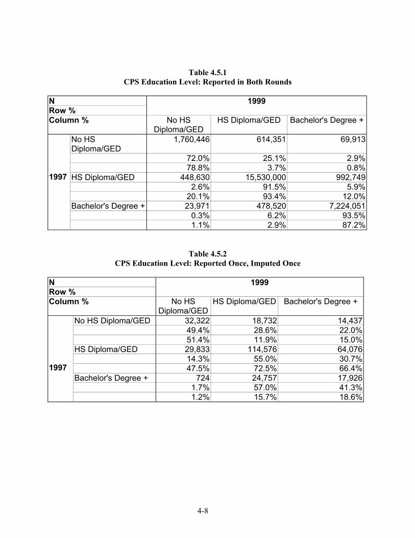
4-8

Table 4.5.1 CPS Education Level: Reported in Both Rounds

N Row %

1999

Column % No HS Diploma/GED

HS Diploma/GED Bachelor's Degree +

No HS Diploma/GED

1,760,446 614,351 69,913

72.0% 25.1% 2.9% 78.8% 3.7% 0.8%HS Diploma/GED 448,630 15,530,000 992,749 2.6% 91.5% 5.9% 20.1% 93.4% 12.0%Bachelor's Degree + 23,971 478,520 7,224,051 0.3% 6.2% 93.5%

1997

1.1% 2.9% 87.2%

Table 4.5.2

CPS Education Level: Reported Once, Imputed Once

N Row %

1999

Column % No HS Diploma/GED

HS Diploma/GED Bachelor's Degree +

No HS Diploma/GED 32,322 18,732 14,437 49.4% 28.6% 22.0% 51.4% 11.9% 15.0%HS Diploma/GED 29,833 114,576 64,076 14.3% 55.0% 30.7% 47.5% 72.5% 66.4%Bachelor's Degree + 724 24,757 17,926 1.7% 57.0% 41.3%

1997

1.2% 15.7% 18.6%

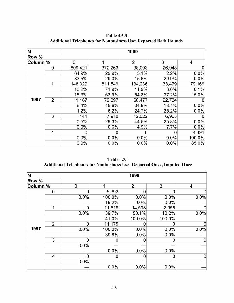
4-9

Table 4.5.3

Additional Telephones for Nonbusiness Use: Reported Both Rounds

N Row %

1999

Column % 0 1 2 3 4 0 809,421 372,263 38,093 26,948 0 64.9% 29.9% 3.1% 2.2% 0.0% 83.5% 29.3% 15.6% 29.9% 0.0%1 148,329 811,549 134,236 33,479 79,169 13.2% 71.9% 11.9% 3.0% 0.1% 15.3% 63.9% 54.8% 37.2% 15.0%2 11,167 79,097 60,477 22,734 0 6.4% 45.6% 34.9% 13.1% 0.0% 1.2% 6.2% 24.7% 25.2% 0.0%3 141 7,910 12,022 6,963 0 0.5% 29.3% 44.5% 25.8% 0.0% 0.0% 0.6% 4.9% 7.7% 0.0%4 0 0 0 0 4,491 0.0% 0.0% 0.0% 0.0% 100.0%

1997

0.0% 0.0% 0.0% 0.0% 85.0%

Table 4.5.4 Additional Telephones for Nonbusiness Use: Reported Once, Imputed Once

N Row %

1999

Column % 0 1 2 3 4 0 0 5,392 0 0 0 0.0% 100.0% 0.0% 0.0% 0.0% — 19.2% 0.0% 0.0% —

1 0 11,518 14,538 2,956 0 0.0% 39.7% 50.1% 10.2% 0.0% — 41.0% 100.0% 100.0% —

2 0 11,175 0 0 0 0.0% 100.0% 0.0% 0.0% 0.0% — 39.8% 0.0% 0.0% —

3 0 0 0 0 0 0.0% — — — — — 0.0% 0.0% 0.0% —

4 0 0 0 0 0 0.0% — — — —

1997

— 0.0% 0.0% 0.0% —

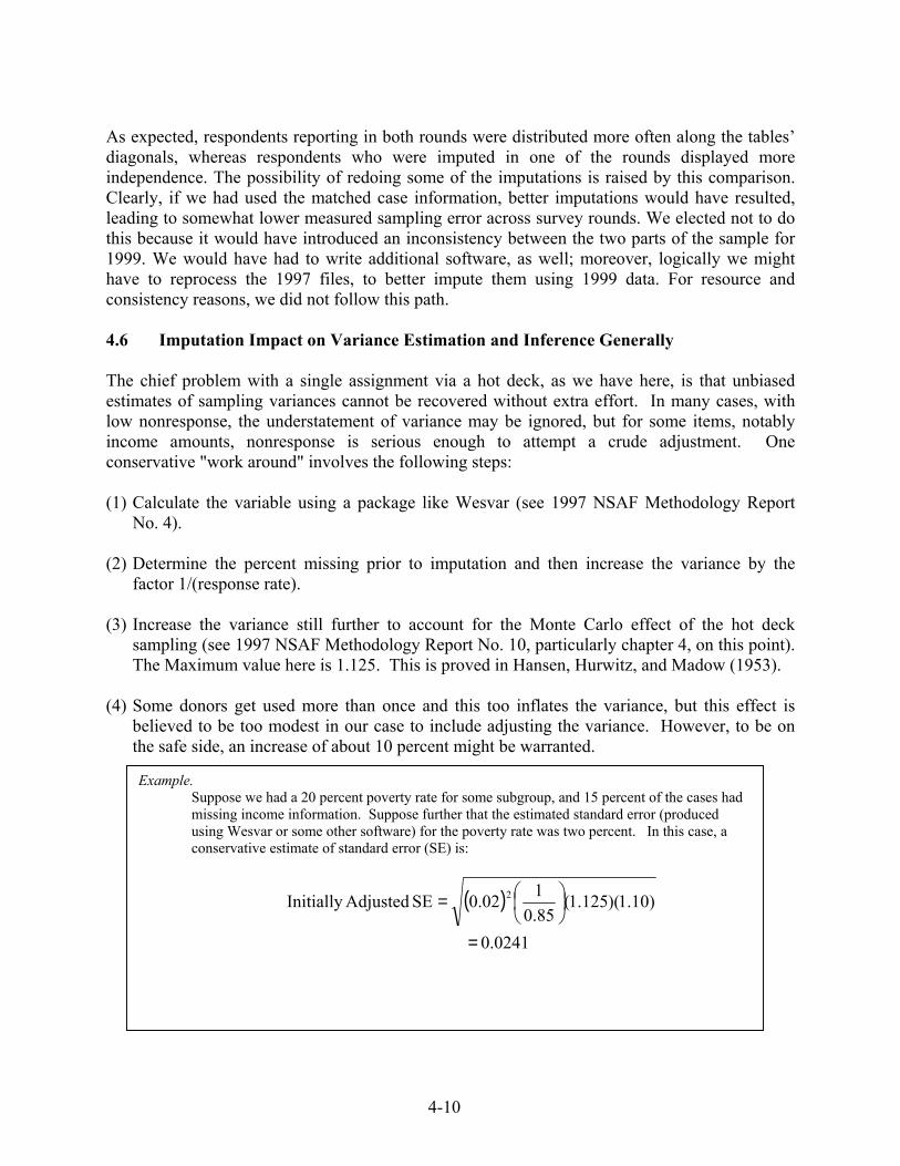
4-10

As expected, respondents reporting in both rounds were distributed more often along the tables’ diagonals, whereas respondents who were imputed in one of the rounds displayed more independence. The possibility of redoing some of the imputations is raised by this comparison. Clearly, if we had used the matched case information, better imputations would have resulted, leading to somewhat lower measured sampling error across survey rounds. We elected not to do this because it would have introduced an inconsistency between the two parts of the sample for 1999. We would have had to write additional software, as well; moreover, logically we might have to reprocess the 1997 files, to better impute them using 1999 data. For resource and consistency reasons, we did not follow this path.

4.6 Imputation Impact on Variance Estimation and Inference Generally The chief problem with a single assignment via a hot deck, as we have here, is that unbiased estimates of sampling variances cannot be recovered without extra effort. In many cases, with low nonresponse, the understatement of variance may be ignored, but for some items, notably income amounts, nonresponse is serious enough to attempt a crude adjustment. One conservative "work around" involves the following steps: (1) Calculate the variable using a package like Wesvar (see 1997 NSAF Methodology Report

No. 4). (2) Determine the percent missing prior to imputation and then increase the variance by the

factor 1/(response rate). (3) Increase the variance still further to account for the Monte Carlo effect of the hot deck

sampling (see 1997 NSAF Methodology Report No. 10, particularly chapter 4, on this point). The Maximum value here is 1.125. This is proved in Hansen, Hurwitz, and Madow (1953).

(4) Some donors get used more than once and this too inflates the variance, but this effect is

believed to be too modest in our case to include adjusting the variance. However, to be on the safe side, an increase of about 10 percent might be warranted.

Example. Suppose we had a 20 percent poverty rate for some subgroup, and 15 percent of the cases had missing income information. Suppose further that the estimated standard error (produced using Wesvar or some other software) for the poverty rate was two percent. In this case, a conservative estimate of standard error (SE) is:

( )

0.0241

)10.1)(125.1(85.0102.0SE AdjustedInitially 2

=

=

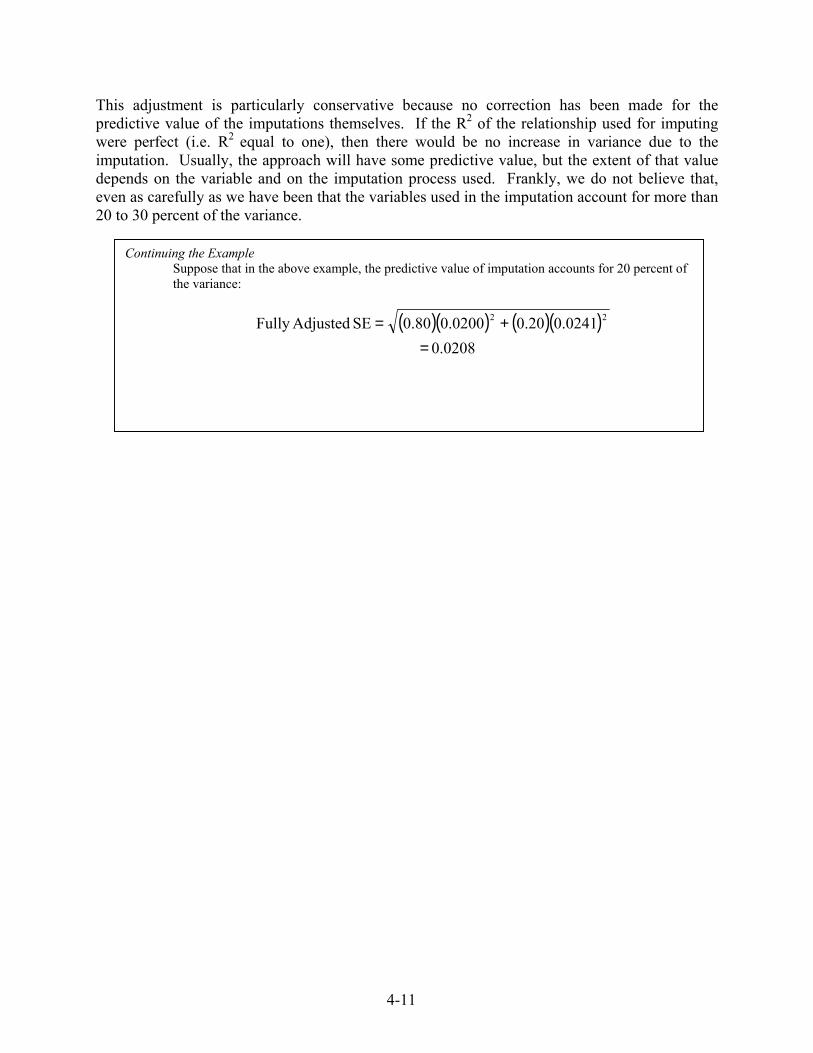
4-11

This adjustment is particularly conservative because no correction has been made for the predictive value of the imputations themselves. If the R2 of the relationship used for imputing were perfect (i.e. R2 equal to one), then there would be no increase in variance due to the imputation. Usually, the approach will have some predictive value, but the extent of that value depends on the variable and on the imputation process used. Frankly, we do not believe that, even as carefully as we have been that the variables used in the imputation account for more than 20 to 30 percent of the variance.

Continuing the Example Suppose that in the above example, the predictive value of imputation accounts for 20 percent of the variance:

( )( ) ( )( )0.0208

0241.020.00200.080.0 SE AdjustedFully 22

=+=

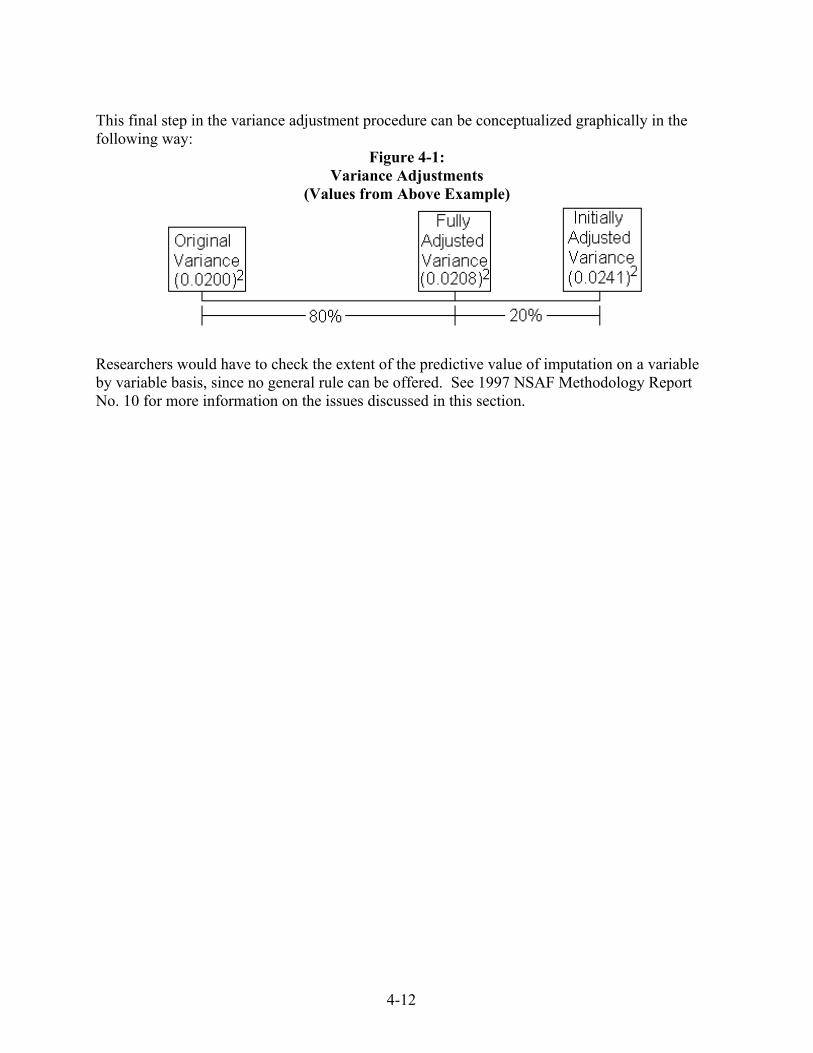
4-12

This final step in the variance adjustment procedure can be conceptualized graphically in the following way:

Figure 4-1: Variance Adjustments

(Values from Above Example)

Researchers would have to check the extent of the predictive value of imputation on a variable by variable basis, since no general rule can be offered. See 1997 NSAF Methodology Report No. 10 for more information on the issues discussed in this section.

A-1

References Andrews, L., Long, S., and Marquis, S. (1997), “Data Cleaning Procedures for the 1993 Robert Wood Johnson Foundation Family Health Insurance Survey.” Santa Monica, CA: RAND. Bassi, F., and Luigi, F. (1997), "Estimators of Nonsampling Errors in Interview-Reinterview Supervised Surveys with Interpenetrated Assignments." Survey Methods and Process Quality. Eds. Lars Lyberg, et al. New York, NY: Wiley and Sons, Inc. Bethlehem, J. (1997), "Integrated Control Systems for Survey Processing." Survey Methods and Process Quality. Eds. Lars Lyberg, et al. New York, NY: Wiley and Sons, Inc. Biemer, P., and Trewin, D. (1997), "A Review of Measurement Error Effects on the Analysis of Survey Data." Survey Methods and Process Quality. Eds. Lars Lyberg, et al. New York, NY: Wiley and Sons, Inc. Carlson, B., Cox, B., and Bandeh, L. (1999), "SAS Macros Useful in Imputing Missing Survey Data." Princeton, NJ: Mathematica Policy Research, Inc. Chapman, D. (1974), An Investigation of Nonresponse Imputation Procedures for the Health and Nutrition Examination Survey. Rockville, MD: Westat. Coder, J. (1999), "Imputation of a Missing Survey Response." (Unpublished) Colledge, M., and March, M. (1997), "Quality Policies, Standards, Guidelines, and Recommended Practices at National Statistical Agencies." Survey Methods and Process Quality. Eds. Lars Lyberg, et al. New York, NY: Wiley and Sons, Inc. Cox, B., and Folsom, R. (1981), "An Evaluation of Weighted Hot Deck Imputation for Unreported Health Care Visits." Proceedings of the Section of Survey Research Methods, American Statistical Association, 1981: 412–417. Dippo. (1997), "Survey Measurement and Process Improvement: Concepts and Integration." Survey Methods and Process Quality. Eds. Lars Lyberg, et al. New York, NY: Wiley and Sons, Inc. Fellegi, I., and Holt, D. (1976), A Systematic Approach to Automatic Edit and Imputation. Journal of the American Statistical Association, 71, 353: 17–35. Ford, B. (1983), "An Overview of Hot-Deck Procedures." Incomplete Data in Sample Surveys, Vol. 2. Burlington, MA: Academic Press, Inc.

A-2

Granquist, L. (1995), "Improving the Traditional Editing Process." Business Survey Methods. Edited by Cox, et al. Wiley and Sons, Inc. Granquist, L., and Kovar, J. (1997), "Editing of Survey Data: How Much is Enough?" Survey Methods and Process Quality. Eds. Lars Lyberg, et al. New York, NY: Wiley and Sons, Inc. Greenlees, J., Reece, W., and Zeischang, K. (1982), "Imputation of Missing Values When the Probability of Response Depends Upon the Variable Being Imputed." Journal of the American Statistical Association 77: 251–261. Groves, R., and Couper, M. (1998), Nonresponse in Household Interview Surveys. New York, NY: Wiley and Sons, Inc. Hansen, M., and Hurwitz, W. (1946), "The Problem for Nonresponse in Sample Surveys." Journal of the American Statistical Association, 41.: 517–529. Hansen, M., Hurwitz, W., and Madow, W. (1953), Sample Survey Methods and Theory (Vol. 2): 129–141. New York, NY: Wiley and Sons, Inc. Holt, T., ed. (1997), Statistical Quality. London: National Statistics Information and Library Service. Jabine, T. (1994), Quality Profile for SASS. United States Department of Education, National Center for Education Statistics. Washington DC. Kalton, G. (1983), Research Report Series: Compensating for Missing Survey Data. Ann Arbor: Survey Research Center, Institute for Social Research, University of Michigan. King, G., Honaker, J. Joseph, A., and Scheve, K. (1998). "Listwise Deletion is Evil: What to Do About Missing Data in Political Science." Paper presented at the Annual Meetings of the American Political Science Association, Boston, MA: September 3-6. Leeuw, E., and Collins, M. (1997), "Data Collection Methods and Survey Quality: An Overview." Survey Methods and Process Quality. Eds. Lars Lyberg, et al. New York, NY: Wiley and Sons, Inc. Lessler, J., and Kalsbeek, W. (1992), Nonsampling Error in Surveys. New York, NY: Wiley and Sons, Inc. Little, R. J. A. 1986. “Survey Nonresponse Adjustments.” International Statistical Review 54: 139–17.

A-3

Little, R., and Rubin, D. (1987), Statistical Analysis with Missing Data. New York, NY: Wiley and Sons, Inc. Lyberg, L., and Kasprzyk, D. (1997), "Some Aspects of Post-Survey Processing." Survey Methods and Process Quality. Eds. Lars Lyberg, et al. New York, NY: Wiley and Sons, Inc. Madow, W., and Olkin, I. (1983), Incomplete Data in Sample Surveys, Volume 2: Proceedings of the Symposium. New York, NY: Academic Press. Madow, W., Nisselson, H. and Olkin, I. (1983), Incomplete Data in Sample Surveys, Volume 1: Report and Case Studies. New York, NY: Academic Press. Madow, W., Olkin, I., and Rubin, D. (1983), Incomplete Data in Sample Surveys, Volume 3: Theory and Bibliographies. New York, NY: Academic Press. Morganstein, D., and Marker, D. (1997), “Continuous Quality Improvement in Statistical Agencies.” Survey Methods and Process Quality. Eds. Lars Lyberg, et al. New York, NY: Wiley and Sons, Inc. Oh, H., and Scheuren, F. with H. Nisselson. (1980a), "Differential Bias Impacts of Alternative Census Bureau Hot Deck Procedures for Imputing Missing CPS Income Data." Proceedings of the Section on Survey Research Methods, American Statistical Association, 1980: 416–420. Oh, H., and Scheuren, F. with G. Shapiro. (1980b), "Estimating the Variance Impact of Missing CPS Income Data." Proceedings of the Section on Survey Research Methods, American Statistical Association, 1980: 408–415. Organizing Committee for the Data Editing Workshop and Exposition, Federal Committee on Statistical Methodology. (1996), Statistical Policy Working Paper 25: Data Editing Workshop and Exposition. Washington, DC: Statistical Policy Office. Pol, F., and Laneheine, P. (1997), "Separating Change and Measurement Error in a Panel Surveys with and Application to Labor Market Data." Survey Methods and Process Quality. Eds. Lars Lyberg, et al. New York, NY: Wiley and Sons, Inc. Rao, J., and Sitter, R. (1997), "Variance Estimation Under Stratified Two-Phase Sampling with Applications to Measurement Bias." Survey Methods and Process Quality. Eds. Lars Lyberg, et al. New York, NY: Wiley and Sons, Inc. Rubin, D. (1977), "Formalizing Subjective Notions about the Effect of Nonrespondents in Sample Surveys." Journal of the American Statistical Association, 72: 538–543. Rubin, D. (1987), Multiple Imputation for Nonresponse in Surveys. New York, NY: Wiley and Sons, Inc.

A-4

Schafer, J. (1997), Analysis of Incomplete Multivariate Data. New York, NY: Chapman & Hall. Scherkenbach, W. (1991), Deming's Road to Continual Improvement. Knoxville, TN: SPC Press. Scheuren, F. (1976), Preliminary Notes on the Partially Missing Data Problem—Some (Very) Elementary Considerations. Delivered at the April 1976 meeting of the Social Security Administration's Statistical Methodology Group. Scheuren, F. (1978), "Discussion of the Paper Entitled, Income Data Collection and Processing for the March Income Supplement to the Current Population Survey, by John Coder." Proceedings of the Data Processing Workshop: Survey of Income and Program Participation: Washington, DC: U.S. Department of Health, Education, and Welfare. Schieber, S. (1978), "A Comparison of Three Alternative Techniques for Allocating Unreported Social Security Income on the Survey of Low-Income Aged and Disabled. American Statistical Association." American Statistical Association, Proceedings of the Section on Survey research Methods: 212-18. Shao, J., Chen Y., and Chen Y. (1998), “Balanced Repeated Replication for Stratifies Multistage Survey Data Under Imputation.” Journal of the American Statistical Association, 93: 818-831. Strudler, M., H.L. Oh, and F. Scheuren. 1986. “Protection of Taxpayer Confidentiality with Respect and to the Tax Model” American Statistical Association, Proceedings of the Section on Survey Research Methods : 375-381. U.S. Census Burea. (1998), Current Report Series p-60, No. 198. Welniak, E., and Coder, F. (1980), A Measure of the Bias in the March CPS Earnings Imputation System and Results of a Sample Bias Adjustment Procedure. American Statistical Association, Proceedings of the Section on Survey Research Methods: 421–425. Williams, R., and Folsom, R. (1981), "Weighted Hot-Deck Imputation of Medical Expenditures Based on a Record Check Subsample." Proceedings of the Section on Survey Research Methods, American Statistical Association: 406–411. Methodological Papers from the 1999 National Survey of America’s Families References for the Papers and Sources used within the papers (Report 7) Adam Safir, Fritz Scheuren, and Kevin Wang (October 2000) National Survey of America's Families: Survey Methods and Data Reliability

A-5

Tamara Black and Adam Safir (August 2000) Assessing Nonresponse Bias in the National Survey of America's Families. In the Joint Statistical Meetings of the American Statistical Association’s 2000 Proceedings of the Section on Survey Research Methods. Kevin Wang (August 2000) Panel Conditioning in a Random-Digit Dial Survey. In the Joint Statistical Meetings of the American Statistical Association’s 2000 Proceedings of the Section on Survey Research Methods. Fritz Scheuren (August 2000) Macro and Micro Paradata for Survey Assessment. In the Joint Statistical Meetings of the American Statistical Association’s 2000 Proceedings of the Section on Survey Research Methods.