2 emtp: modeling and simulation capabilitiesemtp: modeling and simulation capabilities 9 v = r · )...

2C H A P T E R

EMTP Modeling and Simulation Capabilities

21 INTRODUCTION

We begin this chapter with a list of various digital computer programs currently in use for computation of electromagnetic transients in power systems [1 2] We will then give a brief history of EMTP and the versions of it currently existing This is followed by the power system component-modeling capabilities that are provided by a popular version of EMTP Microtran The chapter concludes with the studies that can be carried out using EMTP and certain useful special capabilities The term EMTP is used in this book for various versions of EMTP including Microtran Where it specifically refers to Microtran should be clear from the context Also at some places the words Microtran and mt are used interchangeably mt refers to the transients simulation module of the whole Microtran package

22 DIGITAL COMPUTER PROGRAMS AVAILABLE FOR COMPUTATION OF TRANSIENTS [1]

We give below the originattemptsexisting computer programs for computation of transients in electrical power systems bull Technical University Munich 1963 (first published May 1964) bull Bonneville Power Administration (BPA) EMTP It is a non-commercial version and was

distributed free of cost because of Freedom of Information Act in the USA bull University of British Columbia (UBC) Microtranreg It is a commercial version owned by

UBC and is being distributed by Microtran Power System Analysis Corporation Vancouver Canada

bull NETOMAC Siemens commercial bull Morgat (Electricite de France) commercial bull PSIM (H Jin) commercial Primarily for power electronics studies bull SABER for power electronics studies commercial bull SPICE PSPICE commercial Occasionally used for power electronics

8 Computational Electromagnetic Transients

about the contributions from the UBC Research Group most of which found their way into other versions such as BPA EMTP DCGEPRI EMTP (and later EMTP-RV) and ATP Following are the partial list of contributions bull TACS of Laurent Dube Transient Analysis of Control Systems [5] bull Multiphase untransposed transmission line with constant parameters of K C Lee [6] bull Frequency-dependent transmission line of J R Marti [7] bull Three-phase transformer models of H W Dommel and I I Dommel [8] bull Synchronous machine model of V Brandwajn Type 59 [9] bull Synchronous machine data conversion of H W Dommel [10] bull Underground cable models of L Marti [11] bull New line constants program and improved frequency-dependent line model of J R Marti

[7] EMTP with extensions to detailed HVDC controls was developed by Manitoba HVDC Research Centre Canada It is a commercial version and is called EMTDC TACS model is not currently available in Microtran version of EMTP

Caution Some of the power system software vendors in India also supply their own version of digital computer program for transients and call it as EMTP It must be mentioned here that these programs suffer from unacceptable limitations and the validation methods used for the results they produce may be questionable

A note on terminologyTraditionally the digital computer program for computation of electrical parameters of a transmission line is called Line Constants Program With the implementation of frequency dependence of parameters it is more appropriate to call the program as Line Parameter Evaluation Program However the usage of the name Line Constants Program still continues In this book we will use both the terminologies with the realization that they refer to one and the same program

24 MODELING CAPABILITIES OF EMTP (MICROTRAN VERSION) [12]

In this section we provide basic explanation of models provided by Microtran For specific details such as input data requirement etc the reader should consult Reference 12 The readers who are not familiar with line modeling wave propagation and related topics should first go over the theory behind line modeling presented in Chapter 3

241 Network Branch Elements2411 Lumped Elements24111 Series R L CThis is to be used for the following types of branches without coupling The branch can be a ldquofullrdquo R-L-C series connected or with one or more of the elements missing bull Lumped resistance is described by the equation

EMTP Modeling and Simulation Capabilities 9

v = R i (21) where v and i are the current voltage across and current through the resistance and R is

the value of the resistance bull Lumped inductance is described by the equation v = L didt (22) where v and i are the current voltage across and current through the inductance and L

is the value of the inductance bull Lumped capacitance is described by the equation i = C dvdt (23) where v and i are the current voltage across and current through the capacitance and C

is the value of the capacitance The energy storage elements which are described by differential equations are actually represented by their ldquodiscretized equivalentsrdquo The discretization is done by application of the trapezoidal rule of numerical integration and is explained in Chapter 10 The R-L combination can be used to represent a short transmission line (lt80 km)

24112 CircuitsSingle- and multiphase p circuit models are provided in EMTP to allow representation of transmission lines and transformers when represented as mutually coupled circuits The single-phase p model can be used to represent a balanced (transposed) transmission line in which case the required data will be the positive sequence parameters Rpos Lpos and Cpos See Fig 21

Fig 21 Single-phase p model

The positive sequence parameters can be computed for a practical tower configuration using a Line Parameter Evaluation Program (LPEP) or formulas suitable for hand computations Theory behind LPEP is covered in Chapter 3 and the detailed explanation in Chapter 5 The multiphase p enables the user to represent the coupling between branches for example interphase coupling of a three-phase transmission line or two three-phase circuits on the same tower or two lines in the same right-of-way The multiphase p model assumes that the transmission line by design is constructed symmetrically In this scalars Rpos Lpos and Cpos

become coupled symmetric matrices [R] [L] and [C] in the phase domain ie in abc coordinates Figure 22 shows the three-phase p model connected between two three-phase nodes k (k1 k2 k3) and m (m1 m2 m3)


Fig 22 Three-phase p model

We can visualize the above three-phase multi-p as a ldquomatrix connectionrdquo diagram shown in Fig 23

Fig 23 Matrix connection diagram of three-phase p model

Each of the matrices is symmetrical and has the form as shown below for [R]

[R] = 11

21 22

31 32 33

symmetricRR RR R R

aelig divide divide oslash

(24)

The differential equations describing the p section are given by

[vk] ndash [vm] = [R] [ikm] + [L] kmdidt

[ik] = [ikm] + 1 [ ]2

kdvC

dt

[im] = 1 [ ]2

kdvC

dt

ndash [ikm]

(25)

The interpretations of the elements are as follows Rii + j w Lii = self impedance of branch i (impedance of loop formed by branch i and ground

returnrdquo)


Rik + j wthinspLik = mutual impedance between branches i and k Rik mutual resistance introduced by the presence of ground and it expresses a phase shift between induced voltage and inducing current Rik π 0 with nonzero earth resistivity [See Section 35 for mutual impedance in the presence of ground]

Cii = sum of all capacitances connected to the nodes at both ends of branch i Cik = negative value of capacitance from branch i to branch k [vk] = [vk1 vk2 ordm] [ik] = [ik1 ik2 ordm] [ikm] = [ik1 m1 ik2 m2 ordm] [imk] is similar to [ikm] Note that for a three-phase line the suffixes 1 2 and 3 correspond to phases-a b and c The impedance ([R] + jwthinsp[L]) and capacitance matrix elements for a three-phase line model can be obtained from the corresponding sequence quantities from the following relationships

Z11 = Z22 = Z33 = 13

(Zzero + 2 Zpos )

Z12 = Z13 = Z23 = 13

(Zzero + Zpos )

C11 = C22 = C33 = 13

(Czero + 2 Cpos )

C12 = C13 = C23 = 13

(Czero + Cpos )(26)

where Zzero is the zero sequence impedance and Zpos is the positive sequence impedance which is equal to negative sequence impedance for a static element The derivation of the relationships given in Eq (26) is given in Chapter 3 For computation of parameters of multiphase transmission lines or two lines in the same right-of-way we resort to Line Constants Program mtLine which is included in the Microtran package For steady-state computations such as power flow or for EMTP steady-state solution the nominal p representation can be used The validity of the nominal p model depends on the type of branch element overhead line or underground cable and length The guidelines are given below [13] bull For overhead lines the length up to which nominal p representation is valid is given by

ℓ lt 10000f where f is the frequency which works out to 200 km for 50 Hz and 170 km for 60 Hz

bull For underground cables the length up to which nominal π representation is valid is given by ℓ lt 3000f which works out to 60 km for 50 Hz and 50 km for 60 Hz

Hence lines with medium length (80 km to 200 km) can be represented by nominal p For longer lines we should go in for equivalent p model or cascaded nominal p models For time-domain (transient) solution a number of p sections have to be cascaded and the number depends on the length of the line and maximum frequency that has to be ldquocapturedrdquo in the simulation [14] The number of p sections n can be estimated as follows

n = max444

vf

(27)


For example if the lowest mode (ground mode or zero sequence mode) velocity is 259000 kmsecond and if we are interested in capturing phenomena up to 3000 Hz then the length of the p section cannot exceed 19 km (approximately) Hence to represent a 300 km line we require about 16 nominal p sections of 19 km each The p model can be used for steady state or frequency scan solutions and is not accurate for time-domain (transient) solutions The p model can give rise to spurious oscillations For transient solution frequency-dependent distributed-parameter transmission line models should be used The following results from EMTP simulation [14] (Fig 24) give an idea of inaccuracies incurred by representing transmission lines in terms of p sections

Fig 24 Comparative response of a transmission line with p sections (8 and 32) and a model with a constant parameter distributed parameter line

Another important consideration in modeling transmission lines is the frequency dependence of resistance and inductance parameters The EMTP simulation using constant parameters at power frequency can give rise to very inaccurate results The theory behind inclusion of frequency dependence is explained in Chapter 3 and the model of a transmission line incorporating frequency dependence is given in Section 24124 Microtran provides a high input accuracy option for R L and C which was required in the case of transformer representation by means of inductances calculated from magnetizing and short-circuit inductances After the inverse inductance model of the transformer was implemented this option is no longer required The maximum number of phases that can be modeled is fifty

24113 Inductively and capacitively coupled branchesThese can be modeled as limiting cases of multiphase p circuits


4 You cannot model three ideal transformers in deltadelta connection because two of them are sufficient to define all three line-to-line voltage transformations between phases A to B B to C and C to A

2412 (Continuously) distributed-parameter linesRefer Chapter 3 for theory behind distributed-parameter lines In an actual transmission line the phase and interphase R L and C parameters are continuously distributed as against cascaded π circuits which are discretely distributed The voltage and current in a distributed-parameter line are described by partial differential equations The solutions of the partial differential equations indicate that the voltage and current are actually waves travelling on the transmission line Imagine a transmission line energized at the sending end The voltage will not appear instantaneously at the receiving end since the voltage wave which travels almost at the speed of light will take a finite amount of time to reach the receiving end Hence during the travel time from the sending end to the receiving end the ends remain electrically disconnected This characteristic distinguishes the continuously distributed-parameter line or simply distributed-parameter line The voltages and currents on the N phases of a practical transmission line are functions of location x and time t and are related by the partial differential equations

ndash [ ] [ ]v vL R i

x tpara para = cent + cent para para

ndash [ ] [ ]i iC G v


(28) The prime in R cent Lcent and C cent is used to indicate distributed parameters ie parameters per unit length (for example in Wkm) in contrast to lumped parameters If the parameters R cent Lcent C cent are assumed to be constant ie not dependent on frequency their values can be obtained from Line Constants Program The parameters for the frequency-dependent line model are obtained from the auxiliary program fdData [15] included in the Microtran package

24121 Balanced transmission linesBy construction most of the EHV lines are ldquounbalancedrdquo By that we mean that the mutual couplings between the phases are not equal themselves We can visualize the unbalance by considering some of the common tower configurations given in Fig 27 The above configurations give rise to a series of impedance matrix of the line which will be symmetric but not balanced A balanced matrix is one in which the diagonals (self impedances) are equal among themselves and the off-diagonals (mutual impedances) are equal among themselves Transposition of the line such that each phase conductor occupies all positions in the tower will yield approximately balanced matrix when taken over one transposition cycle The remarks made for series impedance matrix also hold good for shunt capacitance matrices Transposition of transmission lines is dealt with in detail in Chapter 3


There are a number of transformations that decouple N mutually-coupled equations in phase variables to give N uncoupled single-phase equations in modal variables Out of the N equations in the modal domain one equation describes the ground return mode and the remaining Nndash1 equations describe line (sky or aerial) modes The impedances of all Nndash1 line modes are identical for common transformations used in power system analysis In Microtran the transformation matrix used corresponds to 0ab transformation

Note 1 For a three-phase ac line the ground return mode parameters are identical to zero sequence

parameters and the line mode parameters are the positive sequence parameters 2 For a single-phase line the ground return parameters are simply the single-phase parameters

and no line mode parameters exist Modes and modal transformations are explained in Chapter 3

24122 Untransposed transmission linesFor a general untransposed line the series impedance and shunt capacitance matrices are symmetrical but not balanced That is all the diagonals are not equal among themselves and so are all the off-diagonals However we can still create decoupled modes of voltages and currents by making use of modal transformations that are specific to the tower-line geometry We cannot use standard transformation like 0αβ transformation to obtain decoupled modes To model a general untransposed distributed-parameter line in EMTP the user must therefore give the modal transformation matrix in addition to the line parameters in modal domain as input data

Fig 27emsp Commonemsptoweremspconfigurationsemsp(a)emspldquoflatrdquoemspconfigurationemspandemsp(b)emsptriangularemspconfiguration[Reproduced (Fig 27 (a)) from Reference 16 with permission]


Lumped Resistance ModelEMTP expects modewise line parameters for the constant-parameter line Further if the line is untransposed it expects the modal transformation matrix as well Each set of modal parameters constitutes a single-phase line The losses in each of these lines in the lumped resistance model are represented by total resistance of the line split as shown in Fig 210

Fig 210 Lumped resistance model for accounting line losses

In Fig 210 Rtotal = Rcent x length of the line The lumped resistance model is accurate as long as Rtotal is small compared to the surge impedance radic(LcentC centthinsp) This is generally true for the line

Fig 28 Variation of zero sequence parameters with frequency from Reference 17 [Redrawn from Reference 17 with permission]

Fig 29 Variation of positive sequence parameters with frequency from Reference 17 [Redrawn from Reference 17 with permission]


mode For the ground return mode even with frequency dependence of line parameters taken into account lumped resistance model is normally used [12]

Distortionless Line ModelA distortionless line preserves the wave shape of voltage and current from the point of origin of the wave (sending end) to the destination (receiving end) Distortionless line models are seldom used in EMTP simulations because wave propagation in power transmission lines is not distortionless It can be shown that if the line is distortionless the following condition is satisfied

cent cent=

cent centR GL C

(211)

For overhead power lines G cent is very small and its value for distortionless line model is artificially increased to make the line distortionless This naturally increases the shunt loss To make the total line loss constant the series resistance is correspondingly reduced This then implies that

input1

2centcent cent

= =cent cent cent

RR GL C L

(212)

where R input is the input value of line series resistance per unit length The input value of the line series resistance per unit length is automatically halved by EMTP and the halved value is taken as the series resistance The reciprocal of the remaining half is taken as the shunt conductance It can be easily seen that the attenuation constant a for the distortionless is given by

athinsp = input

2R C

Lcent cent

cent (213)

The corresponding decrement factor is endash al with l = length of line The proof of Eq (213) is given in the Appendix to this chapter

Lumped resistance or distortionlessFollowing points will serve as guidelines for the user 1 The lumped-resistance model (at three points) is accurate as long as the line total resistance

is small compared to the surge impedance 2 The lumped-resistance model is the preferred model for constant-parameter line

representations 3 Distortionless line models are seldom used except for positive and negative sequence

line modes but even there the lumped resistance line model is normally more accurateNote ac steady-state solutions at one or more frequencies can be performed by EMTP These are mainly done for the following purposes 1 To provide initial values for subsequent transient solutions tmax gt 0 where tmax is the

maximum time for transient solution


Equation (216) can be rewritten as

Vk ndash ZC Ikm = (Vm + ZC Imk) e (ndash gthinspl) = (Vm + ZC Imk ) A(w) (218)

where we have denoted the propagation factor endash gthinspl as (w) Equation (218) can be rearranged as

Ikm = 1 ndash

aelig + divide oslash

mk mk

C CZ ZV

V I A(w) (219)

In the time domain Eq (219) corresponds to the following expression in

ikm (t) = 1

CZ vk (t) ndash max

min

t

t [vm (t ndash u) + ZC imk (t ndash u)] a(u) du (220)

Note that we now have two travel times tmin and tmax in the case of frequency-dependent parameter line The essence of the J Martirsquos method is as follows 1 Approximate A(w) and ZC (w) by rational functions in the frequency domain The function

A(w) is of the form

Aapprox (s) = endash stmin k 1 2

1 2

( ) ( ) ( )( ) ( ) ( )

n

m

s z s z s zs p s p s p

+ + ++ + +

(221)

2 Expand that portion A(w) that does not include the exponential term as partial fractions 3 The inverse Fourier transform after step 2 yields

aapprox (t) = min1 min 2 min ndash ( ndash )ndash ( ndash ) ndash ( ndash )1 2 mp tp t p t

mk e k e k e tt t+ + for t gethinsptmin

= 0 otherwise 4 Use the expression given in step 3 in place of a (u) in Eq (220) and evaluate the integral

This step gives the past history term for propagation 5 The partial fraction expansion of ZC is interpreted as a set of series connected R-C networks

and a resistance between node k and ground Integrate the capacitance equations using trapezoidal rule to yield an equivalent resistance and a past history term one step behind

6 Combine the past history terms from steps 4 and 5 and place it on the right-hand side [i] and include equivalent conductance (reciprocal of equivalent resistance) in the conductance matrix [G] to solve the set of equations

[G] [v] = [i] (222) Refer to Chapter 8 for more details on the formation and solution of Eq (222) For modeling frequency dependence the data for coefficients of partial fraction expansion of the characteristic admittance and propagation function for each line mode and the current modal transformation matrix should be supplied by the user This can be obtained from the module fdData which produces this data in the form of a file that can be directly read by the transients simulation module mt The modal transformation matrix will be computed at optional user-specified frequency (or a default frequency) by fdData and it will be real and constant


In the frequency-dependent line model the line losses are continuously distributed However in the case of overhead transmission lines in power systems lumped versus distributed modeling of the line losses is not normally a major factor determining the accuracy of the simulation results

24125 Summary of data requirements for line modelingThe basic data requirements for the various models are given below For exact format of the input and other details the reader should consult Reference 12 which gives many illustrative examples for various line models 1 Balanced constant parameter lumped resistance or distortionless line model bull Number of phases of the transmission line (maximum = 50) bull For a double-circuit three-phase line this number would be 6 bull Resistance in ohms per unit length (R cent) whose value can be zero plus bull One of the following data options (a) (b) or (c) for distributed-parameter lines Option (a) nonzero values of bull Inductance in millihenries per unit length (Lcentthinsp) or inductive reactance in ohms

unit length (wLcent) bull Capacitance in microfarads per unit length (C centthinsp) or susceptance in microsiemens

unit length (wC centthinsp) bull Surge impedance (ZC) in ohms Option (b) surge impedance and wave speed Option (c) surge impedance and travel time (t) which must be larger than the step

width used for numerical integration (trapezoidal rule) bull Line length Note (a) The per unit length resistance and data given as options must be specified for ground

and line modes (zero and positive sequence parameters for a three-phase line) (b) Mixing of loss-handling methods (lumped resistance or distortionless) among different

modes is allowed for a multiphase line (c) Constant parameter does not imply that the parameters are at power frequency In

fact the parameters especially zero sequence are to be specified at a much higher frequency for more accurate simulation The frequency to be specified depends on the user judgment A typical value would be around 12 kHz The program mtLinefdData can be used to produce these values In fact fdData produces a file that can be directly read by the transients module mt In this case mt uses 0αβ transformation to diagonalize the impedance matrix The reader should refer to the reference manuals for mtLine and fdData Reference 15 for more details

2 Unbalanced constant parameter lumped resistance or distortionless line model Data for case 1 plus bull Number of phases plus


bull Transformation matrix This matrix is available from fdData module computed at a frequency specified by the user

3 Balanced and untransposed frequency-dependent line parameter model Recall that for the frequency-dependent line model the line parameters are considered to be functions of frequency that is R cent = R cent(w) Lcent = Lcent (w) G cent = G cent (w) and C cent = C cent (w) In practice G cent and C cent are usually constant All the parameters including the losses are modeled as continuously distributed along the linersquos length This model is based on the synthesis by rational functions in the frequency domain of the line propagation function and characteristic impedance as explained earlier The line representation for these models is produced by the auxiliary program fdData in the form of a model data file This file contains the partial fractions expansion of the characteristic admittance and propagation function for each line mode followed by the transpose of the currents modal transformation matrix For a perfectly transposed (and therefore balanced) line the modal parameters are exact at all frequencies using a constant and real transformation matrix eg Clarkersquos transformation matrix [16] The transients simulation module mt recognizes the line as balanced and uses 0ab transformation to convert between phase and modal quantities

242 SwitchesAny switch operation in a power system initiates transients between pre- and post-operation steady states The Microtran provides models for bull time-controlled and bull voltage-dependent switches

2421 Time-controlled switchesFollowing points are to be noted for time-controlled switches bull Circuit breaker poles and similar types of switches whose opening and closing depends

upon time are modeled as time-controlled switches bull The switch resistance is infinite in the open position and zero in the closed position bull In this model the user has to specify the closing (CT ) and opening (OT ) times The

time-domain simulation begins with the switch open if CT ge 0 and with the switch closed if CT lt 0 The latter case indicates that the switch is closed during the steady state The actual switch closing within mt occurs at the time step closest to Tclose (same as CT)

bull The opening of the switch is influenced by OT and another parameter called ldquocurrent margin (CM)rdquo

bull If CM = 0 then within mt the switch opens after the time step closest to Topen as soon as the switch current iswitch has gone through zero If CM gt 0 then the switch opens after the time step closest to Topen as soon as the magnitude of the switch current (|iswitch|) has become less than CM

bull The close-open sequence can be repeated as often as desired by specifying pairs of values Tclose Topen


bull The switch closes after the time step closest to closing time Tclose as soon as the absolute value of the voltage across the switch becomes greater than the breakdown voltage

bull There is another parameter to be specified by the user Tdelay delay time which determines how long the switch remains closed (to simulate persistence of the arc) The switch will open thereafter depending on conditions on current margin explained for time-controlled switch

bull The sequence ldquoclosing time-delay openingrdquo repeats itself after the first and subsequent openings as indicated in the sketch below (Fig 211)

Fig 211emsp Theemsprepeatingemspsequenceemspldquoclosingemsptime-delayemspopeningrdquoemsppointsemspA B and C correspond to zero switch currents with current margin = 0[Redrawn from Reference 12 with permission]

bull The data requirements for the voltage-dependent switch are closing time breakdown voltage time-delay the node from which time-dependent breakdown voltage has to be picked up and current margin

The readers are urged to go through many illustrative examples in Reference 12 which give the input data for switches in the format required by Microtran

243 Nonlinear ElementsBy nonlinear elements we mean resistive and inductive elements that do not have a linear voltage-current relationship For example if an input to a circuit element is a sinusoidal and the output is also a sinusoidal wave of same frequency then the element is linear It is nonlinear otherwise Microtran provides two methods of handling nonlinear elements bull Piecewise linear approximation method bull Compensation method

2431 Piecewise linear method (piecewise linear models)24311 Piecewise linear resistanceSurge arresters are also included in this category provided the characteristics of arrester disks (silicon carbide or metal oxide) can be represented as a piecewise linear slope The piecewise linear characteristic to idealize a given voltage-current characteristic can exhibit two or more than two slopes


243111 Two-slope piecewise linear resistance and surge arrester characteristicsThe voltage-current characteristic of this element is shown in Fig 212(a) It is simulated by the program with a series connection of voltage source slope resistance R and switch as shown in Fig 212(b) The restriction regarding switch connection to nodes with no voltage source connected to it applies to this case also The piecewise linear resistance is ignored (disconnected) during steady-state solution

Fig 212 (a) vndashi characteristic (b) element representation k and m are the nodes between which the element is connected and m is the internal node created by Microtran

[Redrawn from Reference 12 with permission]

Piecewise Linear Resistance bull Note that the element consists of a voltage source a resistance and a switch all connected

in series The operation of the element is straightforward bull The voltage source represents the ldquosaturationrdquo voltage ie the voltage at which the

characteristic changes slope from infinite value to finite value R bull The switch opens (stops conducting) when the current goes to zero and stays open as

long as the voltage across the switch (v) is less than vSATURATION Microtran also provides the value of energy absorbed by the piecewise linear resistance each time the current goes to zero

bull The user can also input the nonzero value of the switch resistance (Rswitch) if it is available

Surge Arrester bull There is another input required from the user for this model sparkover voltage vsparkover

A nonzero value for vsparkover (sparkover voltage of the gapped arrester) results in an approximate model for the arrester A zero value for vsparkover implies a two-slope resistance only

bull The approximation involved in surge arrester model is illustrated by a typical surge arrester characteristic (Fig 213(a)) and the simulated characteristic (Fig 213(b)) shown below

bull For more details the reader should consult Reference 12


As we can see that we have to specify two resistance values and two saturation voltages The first resistance value (60 W) and saturation voltage (150 volts) is input similar to the two-slope case The second of resistance (Rx) is computed as follows

1 1 160 10xR

+ =

which gives Rx = 12 W The saturation voltage (vSATURATION2) is read off from the graph

The corresponding EMTP representation is shown in Fig 215

Fig 215 EMTP representation of piecewise linear resistance characteristic shown in Fig 214 The piecewise linear resistance is connected between nodes 1 and 2


Similar representation can be obtained for piecewise linear resistance for more number of slopes In general the parallel resistance (Rx ndash i) that will give the correct i th slope (Rslope - i ) is given by

slope ndash ( ndash 1) ndash slope ndash

1 1 1

i x i iR R R+ =

(223)

It is obvious that if there are n slopes in the piecewise linear characteristic then the total number of resistors in the EMTP representation would be n and the number of parallel resistors and corresponding saturation voltages will be n ndash 1

Surge Arrester with Characteristic that has More than Two SlopesThe parallel resistance connection method can also be used to realize the surge arrester v ndash i characteristic but the following restrictions apply

1 The characteristic cannot contain a linear slope through the origin This implies that the characteristic shown in Fig 214 is allowed and that shown in Fig 216 is not allowed


Fig 216 A four-slope of piecewise linear resistance characteristic with a linear slope through the origin


2 The sparkover voltage must be lower than the saturation voltage

Note 1 If the characteristic contains a negative slope it is allowed provided a point of intersection

of the characteristic with the Thevenin characteristic of the system at the point of connection of the piecewise linear resistance can be found The reason for this will become clear when we take up the compensation method of handling nonlinear elements The compensation method is explained briefly in Section 2432 A negative resistance with operation in the first and third quadrant could be a crude approximation of an arc characteristic

2 A forced negative resistance operation in the second and fourth quadrants is possible For more details the reader should consult Reference 12 Such a characteristic represents a low-frequency corona model

Table 21 summarizes the modeling options for piecewise linear resistance and surge arrester The data requirements will now include parallel resistance values and corresponding saturation voltages

24312 Piecewise linear inductanceThe simulation of piecewise linear inductance within EMTP is somewhat similar to piecewise linear resistance with flux linkage ndash voltage and resistance ndash inductance being similar quantities A two-slope approximation for the flux linkage (y)-current (i) nonlinear characteristic is shown in Fig 217 The slope of the characteristic going through the origin represents inductance L1 and the next segment represents inductance L2 The simulation of this characteristic within EMTP is illustrated in Fig 218 It is clear that for simulation of inductance L1 the switch in Fig 218 must be open and for simulation of L2 the switch should be closed with Lp given by

2 1

1 1 1

pL L L= +

(224)


Fig 218 Simulation of two-slope of characteristic shown in Fig 217 within EMTP [Redrawn from Reference 12 with permission]

The parallel connection of inductances shown in Fig 218 is special in the sense that the flux in Lp is always calculated by integrating vk ndash vm (rather than vk ndash vm) The flux yp = y1 always independent of the switch position [17] This is because the parallel connection is just to realize the slope L2 and in reality there is only one element How faithfully the simulation ldquotracksrdquo the two-slope characteristic depends on the value of step size of numerical integration Dt In some situations there can be fictitious overshoots when the slope changes from L1 to L2 and undershoots when slope changes from L2 to L1 This is illustrated in Fig 219

Fig 219 Overshoot and undershoot produced while simulating two-slope characteristic (IFLUX = 0)


The overshoots and undershoots can be controlled by specifying a parameter IFLUX to EMTP But the control is obtained at the expense of simulation on a shifted characteristic as shown in Fig 220 Two more important points deserve mention regarding piecewise linear inductance model 1 For transient simulations starting from automatic initialization of flux the piecewise

inductance is modeled as the inductance in the linear region The initial value of the flux


y(0) is computed using this inductance EMTP considers only fundamental frequency sources in the network while performing the steady-state solution for initialization purposes If the initial flux |y(0)| ge ysaturation then a warning message given below is issued

ldquo WARNING ASSUMPTION THAT AC STEADY STATE HAS FUNDAMENTAL FREQUENCY ONLY IS QUESTIONABLE WITH PRECEDING FLUX OUTSIDE LINEAR REGIONrdquo

2 The two-slope characteristic does not exhibit any hysteresis Approximate simulation of hysteresis in EMTP is possible Consult Chapter 6 of Reference 17 for more details

Data requirementsThe initial flux yresidual L1 L2 switch resistance Rswitch and ysaturation For piecewise linear inductance with more than two slopes more parallel inductances are switched in and out and their values have to be computed and given as input Refer [12] for more details and illustrative examples

24313 Power electronic devicesMicrotran version of EMTP provides models for diodes thyristors triacs (anti-parallel thyristors) and gate turn off devices Functionally these are voltage-controlled switches turning ON when the anode to cathode voltage is positive and OFF as soon as the current through the device crosses zero from a positive to a negative value with possible additional delay and current margin Refer [12] for more details

2432 Compensation method24321 GeneralConsider a single nonlinearity eg a gapless lightning arrester or nonlinear resistor connected between a node and ground as shown in Fig 221 We will briefly illustrate how this method works deferring the detailed treatment to Chapter 8

Fig 220 Simulation on a shifted characteristic no over- or undershoots (IFLUX = 1) [Redrawn from Reference 12 with permission]


Fig 221 Nonlinear element connected to node k

Network is first solved without the nonlinear element to obtain the Thevenin equivalent at node k Then bull As shown graphically in Fig 222 the solution for the current through the nonlinear

element is obtained

Fig 222 Nonlinear element and network characteristics

bull The complete solution for the linear part including the ldquoloadingrdquo effect of the nonlinear element is found by superimposing the linear part solution with effect of the nonlinear element as a current source i

There are some important points to be noted regarding bull Number and location of the nonlinear elements bull Artificial disconnection of nonlinearities using ldquostub linesrdquo bull Singularity check in case nonlinear element is the only branch element in the network bull Treatment of nonlinearities in the ac steady-state solution These will be addressed in Chapter 8 Following branch elements can be solved the using compensation method The element characteristic is specified point-by-point If an analytical expression is available for the characteristic compute the dependent variable values at sufficiently closely-spaced independent variable values and give that as the input to EMTP

24322 Nonlinear resistance and simple surge arresterFigure 223 shows a typical discretized characteristic of a nonlinear resistor


of the voltage across the time-varying resistance becomes greater than or equal to vSTART as illustrated in Fig 224 Before the characteristic becomes effective the time-varying resistance R(t) is taken to be infinite

Fig 224 Typical point-by-point characteristic R(t) and illustration of when the R(t) characteristic becomes effective


Data requirementsTime-varying resistance R(t) point-by-point as a piecewise linear characteristic (linear interpolation will be used between points) magnitude of vSTART Note that if vSTART is specified as zero the time-varying characteristic becomes effective at the beginning of transient study [See Reference 12 for more details]

24324 Nonlinear inductanceHere the inductance depends on the current through it This implies that the flux linkage (y)-current (i) characteristic is not linear Microtran requires ythinsp ndash i characteristic to be specified point-by-point Normally the data is not readily available For example if we want to model transformer core nonlinearity the characteristic available will be a point-by-point description of RMS voltage (VRMS) as a function of RMS current (IRMS) The Microtran package contains a utility that converts VRMS ndash IRMS characteristic to ythinspndash i characteristic[See Reference 12 and related documents for more details]

Data requirementsSteady-state values of current (iSTEADY) through and flux linkage (ySTEADY) of the nonlinear inductance and point-by-point values of current (i) and flux linkage (y) The values specified for iSTEADY and ySTEADY decide how the nonlinear inductance is to be treated in ac steady-state solution if the transient study is to start from an internally computed ac steady state The automatic steady-state solution is indicated to EMTP by specifying a negative starting value (TSTART) for the source data The source description is given later in this chapter Following are the interpretations of the values of iSTEADY and ySTEADY within EMTP bull iSTEADY gt 0 and ySTEADY gt 0 The nonlinear inductance will be represented in the steady-

state solution by the inductance of the linear region computed from iSTEADY and ySTEADY This is the normal case


bull iSTEADY = 0 and ySTEADY = 0 These values indicate that the user is not interested in ac steady-state solution (TSTART ge 0) or the nonlinear inductance is to be ignored in the steady-state solution

bull iSTEADY = 0 and ySTEADY gt 0 This implies that the nonlinear inductance is not conducting during steady-state solution but it has a nonzero initial flux linkage The nonzero initial flux linkage will be automatically computed by the program from the voltage across the nonlinear inductance

bull iSTEADY gt 0 and ySTEADY = 0 This case implies that there is a short circuit in steady state and is not permitted EMTP will terminate execution with error message

24325 Groups of metal-oxide surge arresters and other nonlinear elements This branch type was in the earlier versions (for example Reference 16) used for gapless metal-oxide surge arresters with nonlinear characteristics i(v) of the form

i = ref

| | signv vv

a

(225)

Currently Microtran offers this branch type along with the group that includes time-varying resistances as well as nonlinear resistances and nonlinear inductances The nonlinear resistance and inductance element characteristics are required in the piecewise linear form The subroutine CONNEC in which each group of nonlinear elements is solved can also be modified by the user for user-developed models which require multiphase network connections In contrast to the nonlinear elements of Sections 24322 to 24324 the nonlinear elements of this type can be connected to the network without requiring separation by travel time [See Reference 12 for more details]

244 Voltage and Current Sources2441 GeneralMicrotran provides for three types of source modeling bull Frequently used standard functions for voltage or current sources that are built into the

program bull Functions of arbitrary shape (up to ten) defined point-by-point at discrete time steps Dt

2Dt ordm These values define the functional relationship with respect to time bull User-defined functions in a user-supplied subroutine as explained in Section 915 of

Reference 12 Only salient features are discussed in this section [See Reference 12 for more details] Following are the general points which the user must be aware of 1 Generally all sources are connected between node and local ground However there can

be occasions when sources are to be connected between nodes These and other cases are discussed below


(ii) connect the voltage source between the node extra and ground (iii) connect an ideal transformer with unity ratio between ldquoextrardquo node and ground

on one side (say primary side) and connect the secondary side between nodes k and m See Fig 227(b)

Fig 227 (b) Representation of voltage source with zero internal resistance between two nodes[Redrawn from Reference 12 with permission]

Voltage source has a nonzero internal inductance Li

A voltage source with nonzero internal inductance between two nodes can be represented in a similar fashion with the internal inductance Li between nodes k and m and current source between the nodes that depends on the initial conditions as explained below

Let the voltage be given by v(t) = Vmax cos (wt + j) (226)

(i) If the case starts from zero initial conditions then the current is obtained by integrating the voltage

i(t) = 0

1 ( )t

i

v t dtL

which gives

i(t) = max

w i

VL

[sin(wt + j) ndash sin j] (227)

(ii) If the case starts from linear ac steady state then

i(t) = max

w i

VL

[cos(wt + j) ndash 90deg (228)

Fig 227 (a) Representation of voltage source with nonzero internal resistance between two nodes



The current source i(t) between nodes k and m is then represented as explained next (d) Current source between two nodes The current source between two nodes is represented as two current sources one at

each node as shown in Fig 228

Fig 228 Representation of current source between two nodes [Redrawn from Reference 12 with permission]

Here the current source between nodes A and B is represented as two current sources one out of node A and the other into node B

(e) Voltage and current source at the same node If voltage and current sources are specified at the same node the voltage sources

override and the current sources are ignored Current sources do not influence the network in this case because they are directly short-circuited through the voltage sources

2 The source functions specified by the user must observe consistency in units for example if the voltage sources are specified as volts V (or kilovolts) then current sources should be amperes (or kiloamperes)

3 All built-in source functions have ldquostartrdquo and ldquostoprdquo time parameters Depending on the source type these parameters have certain restrictions and default values These built-in source functions are zero between 0 le t le TSTART and for t ge TSTOP These two parameters enable the user to specify a composite source function synthesized from the recipe of built-in functions as illustrated in Fig 229

Fig 229 A composite source function synthesized from two built-in source functions [Redrawn from Reference 12 with permission]


2442 Standard source functions in-built into EMTPFollowing are the built-in functions in Microtran available to the user 1 Step Function Function description a (t) = Amax for TSTART le t le TSTOP

= 0 otherwise(229)

This function can be used to (i) approximate step functions in the case of zero initial conditions The function is an

approximation because it has a finite rise time Δt 2 with the CDA scheme [18 19] See Fig 230(a)

(ii) represent dc source function with a (0) = Amax with nonzero initial conditions as shown in Fig 230(b) For the nonzero initial conditions other sources and the branches should also have correct dc initial conditions

Fig 230 Step function implementation in Microtran (a) zero initial conditions (b) nonzero initial conditions


The CDA scheme is explained in Chapter 10 The steady-state computations will not be performed for dc sources and as mentioned

earlier approximate dc steady state is obtained with a very low frequency ac sources Consequently the parameters TSTART lt 0 has no meaning for dc sources and is set to zero by the program Consult Reference 12 for more details

2 Rectangular Ramp Function Function description a (t) = 0 for 0 le t le TSTART

= max

0

AT

(t ndash TSTART) for TSTART lt t le TSTART + T0

= AMAX for TSTART + T0 lt t le TSTOP

(230) In this case also TSTART lt 0 has no meaning and is set to zero by the program See

Fig 231 for illustration


Fig 231 Rectangular ramp function implementation in Microtran [Redrawn from Reference 12 with permission]

3 Triangular Ramp Function See Fig 232 for illustration of the function

Fig 232 Triangular ramp function implementation in Microtran (a) general case (b) special case


Function description for the general case a (t) = 0 for 0 le t le TSTART

= MAX

0

AT

aelig divide oslash


= MAX 1START 0

1 0

ndashndash ( ndash )

ndashA A

t T TT T


+ AMAX for t gt TSTART + T0

(231)

In this case also TSTART lt 0 has no meaning and is set to zero by the program

4 Sinusoidal Function See Fig 233 for illustration Function description A general sinusoidal function should include a initial phase angle

with respect to a chosen reference In Microtran the initial phase angle can be provided in terms of degrees or seconds The latter case would imply that the initial phase angle is wthinsptimes initial phase angle in seconds Here w = 2pf where f = frequency of the sinusoidal


It was later realized that the double-exponential surge function of Eq (233) is not adequate to represent short surges such as 820 ms Also the maximum slope dadt occurs as per the measurements close to the peak value whereas for the double-exponential it occurs at t = 0 In order to accommodate the above and other requirements Microtran provides a variety of surge functions which can be categorized as follows

Single- and Double-exponential Surge Function The double-exponential surge function is defined by Eq (233) and restricted to be nonzero between TSTART and TSTOP as shown below

a (t) = AMAX (endashat ndash endashbt) TSTART le T le TSTOP (233)

Surge Function of Standler This function is proposed basically to facilitate representation of short surges as given in relevant IEC and IEEE standards bull Surge function of CIGRE bull Surge function of Heidler There are sub-categories of the first second and fourth functions We give below the sub-categories of the first function For others to refer [12]

Sub-categories of Single and Double-exponential Functions 1 Double-exponential surge function with input values for a and b

2 Double-exponential surge function with input values for 30 90 ldquovirtual front timerdquo and ldquovirtual time to half-valuerdquo


4 Double-exponential surge function with input values for ldquorise timerdquo and ldquofull width at half maximumrdquo

5 Double-exponential surge function with input values for ldquocrest timerdquo and ldquotime to half-valuerdquo

For each sub-category a and b values can be read off from Table 22 [17]

Table 22

T1 T2 (μs) 1 (μs) 1β (μs) AMAX to produce max a(t) = 10

125 348 08 20141250 682 0405 103712200 284 0381 1010

2502500 2877 104 11752502500 3155 625 1104


Note (i) The first four entries correspond to lightning impulse and the last one to switching impulse

The first column of the last entry is Tcr T2 (ii) For the first four entries T1= virtual front time typically 12 ms plusmn 30 T2 = virtual time

to half typically 50 ms plusmn 20 (iii) For the fifth entry Tcr = time to crest typically 250 ms plusmn 20 T2 = virtual time to half

typically 2500 ms plusmn 60

2443 Current controlled dc voltage sourceBrief introduction to HVDC link control bull Voltage regulation and current regulation is kept distinct and assigned to separate terminals bull Normal operation rectifier on constant current (CC) control and inverter on constant

extinction angle control (CEA) with adequate commutation margin This is normally referred to as mode 1 in HVDC literature

bull Rectifier and inverter control characteristics with quantities measured at the rectifier end are shown in Fig 235

Fig 235emsp Rectifieremspandemsp inverteremsp characteristicsemspwithemspvoltageemspandemspcurrentemspmeasuredemspatemsp theemsprectifieremsp endemspVdcemsp asympemspVRECTIFIER = ndash VINVERTER

bull Rectifier characteristic can be moved horizontally by varying current order (IORDER) which is the set point for link current The measured link current is maintained at IORDER by varying ignition angle (also known as firing angle) a See Fig 236 for illustration of IORDER

bull Inverter characteristic can be raised or lowered by changing the transformer tap position at the inverter end A change in transformer tap causes a change in inverter extinction angle g The constant extinction angle regulator at the inverter brings back g to the original value

bull The direct current which changes due to voltage change (due to tap change) is quickly restored by constant current regulator at the rectifier by adjusting a

bull The rectifier tap changer acts to bring a within the desired range (typically amin= 10deg to amax= 20deg)


The current controlled dc source implemented in Microtran consists of a current regulator shown in Fig 237

Fig 237 Model of the current controller implemented in Microtran [Redrawn from References 12 and 17 with permission]

The transfer function G(s) is given by

G (s) = 2

1 3

(1 )(1 ) (1 )

K sTsT sT

++ +

(235)

with limits placed on the output ea in accordance with rectifier minimum firing angle and inverter minimum extinction angle The dc voltage Vdc is a function of ea and is given by Vdc = k1 + k2 ea (236)

See Fig 238 On comparison of Eq (236) with Eq (234) we see that ea is related to a through a cosine relationship Actually ea minus a bias value is proportional to cos a and as shown in Fig 238 Observe that k1 is negative The maximum and minimum limits on dc voltage is due to the limits on ea

Fig 238 Variation of Vdc with ea

From the current controller model of Fig 237 and the transfer function given by Eq (235) we can derive the following differential equation for ea

(T1 + T3) 2

2 1 3 2

( ndash )( ndash ) ndash ndasha a

a= + BIASBIAS

de d I i d eK I i KT T T e

dt dt dt (237)


The limiter on the transfer function indicates that it is a limiter without windup Hence if the converter operates at the maximum limit eathinspmax (or at the minimum limit eathinspmin) either in initial steady state or later during the transient simulation it will back off the limit as soon as the derivative deadt becomes negative (or positive) in Eq (237) The second derivative of ea is zero at the limit

Computation of steady-state dc initial conditionsTo compute the initial steady-state conditions the user should specify among other things initial dc voltage measured at some point in the link (could be one end) and dc current We will explain why dc current is required to be specified later With the specified value of Vdc (0) actually a very low frequency ac solution is performed with Vdc = Vdc (0) cos 2pthinspflow t with flow= 0001 Hz This trick produces results sufficiently close to actual dc solution The ac steady-state solution is explained in Chapter 8 Initial steady-state dc current Idc(0) is required to compute the dc voltage source between two nodes where one node is not ground Actually the steady-state module calculates the initial condition i(0) for the dc current from the specified dc voltages Vdc(0) but its value is not readily available in the program where it is first needed for representation of dc voltage source between two nodes With the specified Idc(0) for the representation of the converter station the voltage source is computed from Vdc (0) = Vsource ndash Requiv Idc (0) (238)and then converted to current source in parallel with Requiv as given below Isource = Vsource Requiv (239)

Requiv is the resistance of the link from the converter station to the point where the initial dc quantities specified are measured See Fig 239

Fig 239 Representation of the converter station for steady-state solution [Redrawn from Reference 12 with permission]

The set point IBIAS of the current controller is automatically computed within the program as

IBIAS = i (0) + (0)eK

a (240)

which is obtained by setting the derivatives of ea to zero in Eq (237)


bull Special types of power flow problems that involve untransposed lines single-circuit double-circuit single-phase distribution lines connected to three-phase substations etc [1] Such cases cannot be solved with classical power flow programs which assume that the power system is completely ldquobalancedrdquo all voltages and currents symmetrical and represented by the single-phase positive sequence network only

bull Special types of short-circuit problems that require the phase shift delta-wye transformers to be taken into account simulation of simultaneous faults

252 Simulation Capabilities of Time-Step Solution ModuleThe simulation capabilities of time-step solution module of EMTP can be categorized as follows bull Transients associated with electric circuits bull Transients in power systems associated with lightning bull Transients in power systems associated with switching bull Electromagnetic transients involving synchronous and induction machines

2521 Transients associated with electric circuitsSome of the problems associated with power system transients can be solved with a circuit-model of the system consisting of lumped elements Such models are amenable to closed-form solution but a number of assumptions are required to make the problem tractable This approach is very well illustrated in Reference 20 It provides physical visualization of the system response and develops the engineerrsquos ability to qualitatively predict the response EMTP provides for this level of modeling and it is the lowest level of modeling sophistication provided by it

2522 Transients in power systems associated with lightningComputation of lightning transients is essential in evaluating surge arrester protection and insulation coordination of air- and gas-insulated substations

2523 Transients in power systems associated with switchingIntended and inadvertent switching can cause very high overvoltages especially in extra high voltage power systems Computation of switching overvoltages is essential in designing the countermeasures for them They are also required for insulation coordination

253 Electromagnetic Transients Involving Synchronous and Induction MachinesThe necessity of adding detailed synchronous machine models to EMTP was first recognized when there were attempts to simulate the occurrence of subsynchronous resonance (SSR) in series compensated lines radially connected to a generating station The SSR caused the destruction of shaft section of a tandem-compounded turbo-generator [21] Transient SSR studies can be conveniently carried out using Microtran Microtran also provides a detailed induction machine model which facilitates accurate simulation of induction switching and reswitching transients in industrial systems and power plant auxiliary systems


28 SUMMARY

This chapter begins with a list of computer programs available for simulation of electrical transients in power systems and traces the history of EMTP development for approximately past fifty years It also provides the modeling capabilities of various EMTP versions in general and Microtran in particular The simulation capabilities and power system studies that can be carried out using EMTP form the concluding part of this chapter

REFERENCES

1 Hermann W Dommel Introduction to the Use of MicroTran and other EMTP Versions Department of Electrical and Computer Engineering The University of British Columbia Vancouver B C Canada (WWW httpwwweceubcca) 1988 Microtran is a registered trademark of Microtran Power System Analysis Corporation Canada

2 Hermann W Dommel ldquoPast Present and the Future of Electric Power Systems from my Perspectiverdquo Zagreb April 20 2007

3 DJ Mader ldquoHistory of the Development Coordination Grouprdquo EMTP REVIEW Vol 1 No1 University of Wisconsin Madison July 1987

4 CanAm EMTP News Vol 88-1 Editor Thomas Grebe USA 5 L Dubeacute and HW Dommel ldquoSimulation of control systems in an electromagnetic transients

program with TACSrdquo Proc IEEE PICA Conf pp 266ndash271 May 1977 6 KC Lee Lightning Surge Propagation in Overhead Lines and Bus-Ducts and Cables

PhD Thesis The University of British Columbia Vancouver Canada July 1980 7 JR Marti ldquoAccurate modelling of frequency-dependent transmission lines in

electromagnetic transients simulationsrdquo IEEE Trans Power App Syst Vol PAS-101 pp 147-157 Jan 1982

8 V Brandwajn HW Dommel and 11 Dommel ldquoMatrix representation of three-phase N-winding transformers for steady state and transient studiesrdquo IEEE TransVol PAS-101 pp 1369-1378 June 1982

9 V Brandwajn Synchronous Generator Models for Simulation of Electromagnetic Transients PhD Thesis The University of British Columbia Vancouver Canada July 1977

10 HW Dommel ldquoData conversion of synchronous machine parametersrdquo EMTP NEWSLETTER Vol 1 No 3 1980

11 L Marti ldquoSimulation of transients in underground cables with frequency-dependent modal transformation matricesrdquo IEEE Trans Vol 3 pp 1039-1110 July 1988

12 Microtran Power System Analysis Corporation MicroTran Reference Manual Transients Analysis Program for Power and Power Electronic Circuits Last revision January 2002 Canada

13 P Kundur Power System Stability and Control McGraw-Hill 1994 USA


14 JC Das Transients in Electrical Systems Analysis Recognition and Mitigation McGraw-Hill Companies New York 2010 p 81

15 Microtran Power System Analysis Corporation MtLine amp fdData Reference Manual Overhead line parameter and model generation support programs for Microtran simulations Published September 1992 Last revision February 2005 Canada

16 HW Dommel and II Dommel Transients Program Userrsquos Manual Copyright 1976 Latest revision Aug 1 1978 The University of British Columbia Vancouver BC Canada V6T 1W5 Last revision January 2002 Canada

17 Hermann W Dommel EMTP THEORY BOOK Second Edition Microtran Power System Analysis Corporation Vancouver British Columbia Canada May 1992 Last update April 1996

18 JR Marti and J Lin ldquoSuppression of numerical oscillations in the EMTPrdquo IEEE Trans Power Systems Vol 4 pp 739ndash747 May 1989

19 J Lin and J R Marti ldquoImplementation of the CDA procedure in the EMTPrdquo IEEE Trans Power Systems Vol 5 pp 394ndash402 May 1990

20 Allan Greenwood Electrical Transients in Power Systems John Wiley amp Sons 1991 21 JW Ballance and S Goldberg ldquoSubsynchronous Resonance in Series Compensated

Transmission linesrdquo IEEE Trans Power App and Syst Vol PAS-92 pp1649ndash1658 SepOct 1973

22 EMTP DCGEPRI EMTP REVIEW Vol 4 No 2 April 1990 University of Wisconsin Madison USA

23 JM Prousalidis et al On Studying Ship Electric Propulsion Motor Driving Schemes Electrical and Computer Engineering Dept National Technical University of Athens Iroon Politechniou 9 15780 Zografou Greece

24 EW Kimbark Electrical Transmission of Power and Signals John Wiley amp Sons New York USA 1949

Appendix

A1 Line of Low Attenuation and Low Distortion-Proof of Eq (213) [24]If the line is distortionless the following condition is satisfied

R GL C

cent cent=

cent cent (211)

For a low distortion and low attenuation R cent ltlt wL cent and G cent ltlt wC cent (A11) The series impedance per unit length is given by (see Fig A11)

Z cent = ndash12 2 2 cot

centw centcent + w centRLjR L e (A12)


= 1ndash

2 2G RC LjL C e

p cent cent aelig + divide oslashw cent w cent w cent cent

Let j =

12

G RC Lcent centaelig + divide oslashw cent w cent

The attenuation constant is given by

a = Re cos ndash2

L C paelig g = w cent cent j divide oslash

Expanding the cosine in the above equation and using approximations for line of low attenuation and distortion we get

a = 12

G RL CC Lcent centaelig w cent cent + divide oslashw cent w cent

or

a = 2 2G L R C

C Lcent cent cent cent

+cent cent (A18)

Dropping the first term in comparison with the second and setting R cent = R input 2 we get Eq (213)


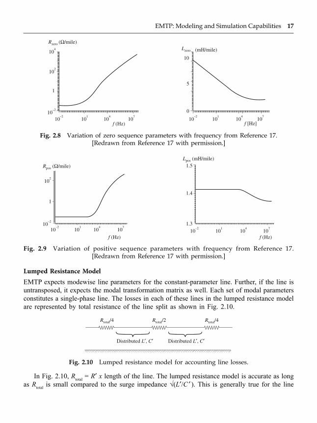
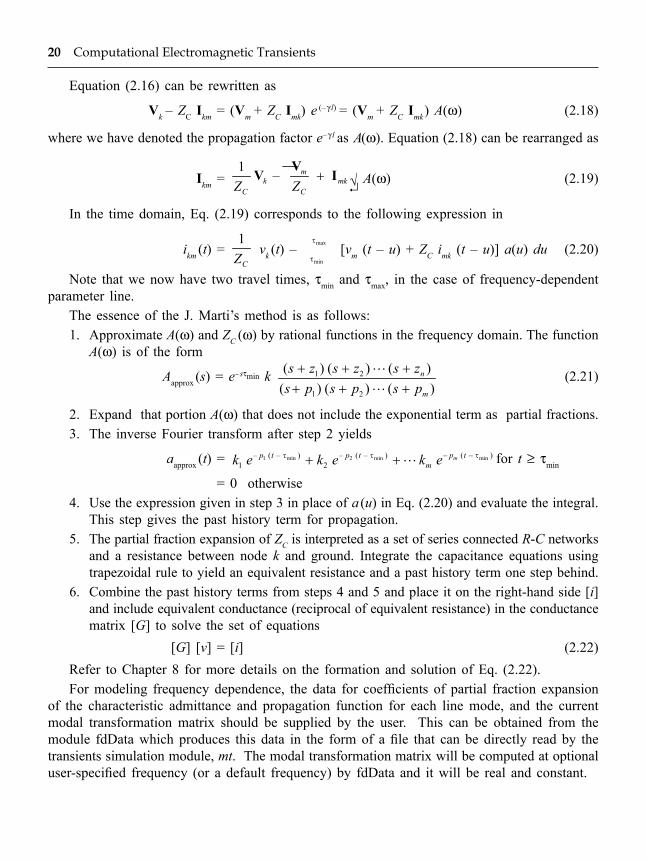
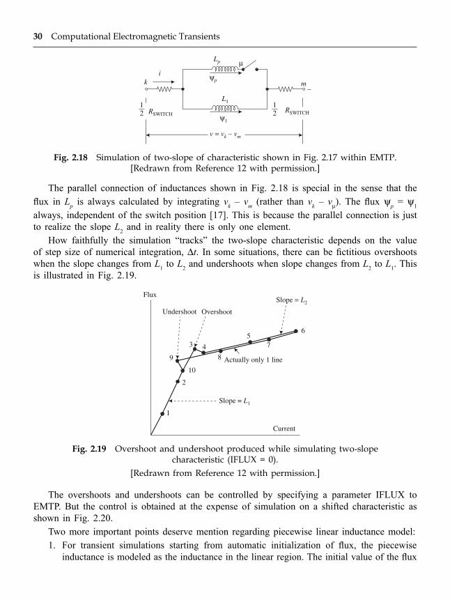
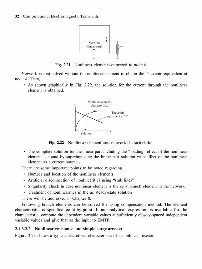
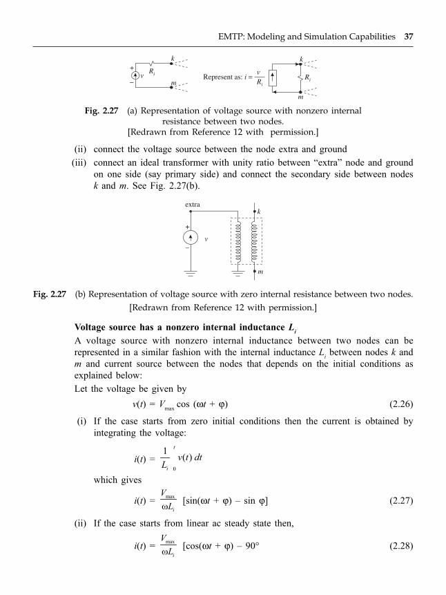
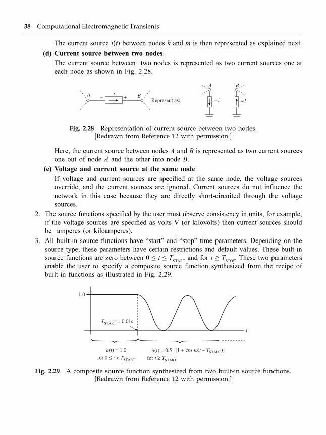about the contributions from the UBC Research Group most of which found their way into other versions such as BPA EMTP DCGEPRI EMTP (and later EMTP-RV) and ATP Following are the partial list of contributions bull TACS of Laurent Dube Transient Analysis of Control Systems [5] bull Multiphase untransposed transmission line with constant parameters of K C Lee [6] bull Frequency-dependent transmission line of J R Marti [7] bull Three-phase transformer models of H W Dommel and I I Dommel [8] bull Synchronous machine model of V Brandwajn Type 59 [9] bull Synchronous machine data conversion of H W Dommel [10] bull Underground cable models of L Marti [11] bull New line constants program and improved frequency-dependent line model of J R Marti

[7] EMTP with extensions to detailed HVDC controls was developed by Manitoba HVDC Research Centre Canada It is a commercial version and is called EMTDC TACS model is not currently available in Microtran version of EMTP

Caution Some of the power system software vendors in India also supply their own version of digital computer program for transients and call it as EMTP It must be mentioned here that these programs suffer from unacceptable limitations and the validation methods used for the results they produce may be questionable

A note on terminologyTraditionally the digital computer program for computation of electrical parameters of a transmission line is called Line Constants Program With the implementation of frequency dependence of parameters it is more appropriate to call the program as Line Parameter Evaluation Program However the usage of the name Line Constants Program still continues In this book we will use both the terminologies with the realization that they refer to one and the same program

24 MODELING CAPABILITIES OF EMTP (MICROTRAN VERSION) [12]

In this section we provide basic explanation of models provided by Microtran For specific details such as input data requirement etc the reader should consult Reference 12 The readers who are not familiar with line modeling wave propagation and related topics should first go over the theory behind line modeling presented in Chapter 3

241 Network Branch Elements2411 Lumped Elements24111 Series R L CThis is to be used for the following types of branches without coupling The branch can be a ldquofullrdquo R-L-C series connected or with one or more of the elements missing bull Lumped resistance is described by the equation















[R] = 11

21 22

31 32 33

symmetricRR RR R R


(24)



[ik] = [ikm] + 1 [ ]2

kdvC

dt

[im] = 1 [ ]2

kdvC

dt

ndash [ikm]

(25)


returnrdquo)




Z11 = Z22 = Z33 = 13

(Zzero + 2 Zpos )

Z12 = Z13 = Z23 = 13

(Zzero + Zpos )

C11 = C22 = C33 = 13

(Czero + 2 Cpos )

C12 = C13 = C23 = 13

(Czero + Cpos )(26)





n = max444

vf

(27)































cent cent=

cent centR GL C

(211)


input1

2centcent cent

= =cent cent cent

RR GL C L

(212)


athinsp = input

2R C

Lcent cent

cent (213)











Ikm = 1 ndash


mk mk

C CZ ZV

V I A(w) (219)


ikm (t) = 1

CZ vk (t) ndash max

min

t



A(w) is of the form


1 2

( ) ( ) ( )( ) ( ) ( )

n

m


+ + ++ + +

(221)





















































1 1 160 10xR

+ =







1 1 1

i x i iR R R+ =

(223)













2 1

1 1 1

pL L L= +

(224)



















element is obtained


















i = ref

| | signv vv

a

(225)















i(t) = 0

1 ( )t

i

v t dtL

which gives

i(t) = max

w i

VL



i(t) = max

w i

VL
















= 0 otherwise(229)









= max

0

AT











= MAX

0

AT

aelig divide oslash


= MAX 1START 0

1 0


ndashA A

t T TT T



(231)















Table 22


125 348 08 20141250 682 0405 103712200 284 0381 1010

2502500 2877 104 11752502500 3155 625 1104


















G (s) = 2

1 3

(1 )(1 ) (1 )

K sTsT sT

++ +

(235)





(T1 + T3) 2

2 1 3 2


a= + BIASBIAS


dt dt dt (237)







IBIAS = i (0) + (0)eK

a (240)











28 SUMMARY


REFERENCES


























Appendix


R GL C

cent cent=

cent cent (211)





= 1ndash

2 2G RC LjL C e


Let j =

12



a = Re cos ndash2



a = 12


or

a = 2 2G L R C


+cent cent (A18)
















[R] = 11

21 22

31 32 33

symmetricRR RR R R


(24)



[ik] = [ikm] + 1 [ ]2

kdvC

dt

[im] = 1 [ ]2

kdvC

dt

ndash [ikm]

(25)


returnrdquo)




Z11 = Z22 = Z33 = 13

(Zzero + 2 Zpos )

Z12 = Z13 = Z23 = 13

(Zzero + Zpos )

C11 = C22 = C33 = 13

(Czero + 2 Cpos )

C12 = C13 = C23 = 13

(Czero + Cpos )(26)





n = max444

vf

(27)































cent cent=

cent centR GL C

(211)


input1

2centcent cent

= =cent cent cent

RR GL C L

(212)


athinsp = input

2R C

Lcent cent

cent (213)











Ikm = 1 ndash


mk mk

C CZ ZV

V I A(w) (219)


ikm (t) = 1

CZ vk (t) ndash max

min

t



A(w) is of the form


1 2

( ) ( ) ( )( ) ( ) ( )

n

m


+ + ++ + +

(221)





















































1 1 160 10xR

+ =







1 1 1

i x i iR R R+ =

(223)













2 1

1 1 1

pL L L= +

(224)



















element is obtained


















i = ref

| | signv vv

a

(225)















i(t) = 0

1 ( )t

i

v t dtL

which gives

i(t) = max

w i

VL



i(t) = max

w i

VL
















= 0 otherwise(229)









= max

0

AT











= MAX

0

AT

aelig divide oslash


= MAX 1START 0

1 0


ndashA A

t T TT T



(231)















Table 22


125 348 08 20141250 682 0405 103712200 284 0381 1010

2502500 2877 104 11752502500 3155 625 1104


















G (s) = 2

1 3

(1 )(1 ) (1 )

K sTsT sT

++ +

(235)





(T1 + T3) 2

2 1 3 2


a= + BIASBIAS


dt dt dt (237)







IBIAS = i (0) + (0)eK

a (240)











28 SUMMARY


REFERENCES


























Appendix


R GL C

cent cent=

cent cent (211)





= 1ndash

2 2G RC LjL C e


Let j =

12



a = Re cos ndash2



a = 12


or

a = 2 2G L R C


+cent cent (A18)





Z11 = Z22 = Z33 = 13

(Zzero + 2 Zpos )

Z12 = Z13 = Z23 = 13

(Zzero + Zpos )

C11 = C22 = C33 = 13

(Czero + 2 Cpos )

C12 = C13 = C23 = 13

(Czero + Cpos )(26)





n = max444

vf

(27)































cent cent=

cent centR GL C

(211)


input1

2centcent cent

= =cent cent cent

RR GL C L

(212)


athinsp = input

2R C

Lcent cent

cent (213)











Ikm = 1 ndash


mk mk

C CZ ZV

V I A(w) (219)


ikm (t) = 1

CZ vk (t) ndash max

min

t



A(w) is of the form


1 2

( ) ( ) ( )( ) ( ) ( )

n

m


+ + ++ + +

(221)





















































1 1 160 10xR

+ =







1 1 1

i x i iR R R+ =

(223)













2 1

1 1 1

pL L L= +

(224)



















element is obtained


















i = ref

| | signv vv

a

(225)















i(t) = 0

1 ( )t

i

v t dtL

which gives

i(t) = max

w i

VL



i(t) = max

w i

VL
















= 0 otherwise(229)









= max

0

AT











= MAX

0

AT

aelig divide oslash


= MAX 1START 0

1 0


ndashA A

t T TT T



(231)















Table 22


125 348 08 20141250 682 0405 103712200 284 0381 1010

2502500 2877 104 11752502500 3155 625 1104


















G (s) = 2

1 3

(1 )(1 ) (1 )

K sTsT sT

++ +

(235)





(T1 + T3) 2

2 1 3 2


a= + BIASBIAS


dt dt dt (237)







IBIAS = i (0) + (0)eK

a (240)











28 SUMMARY


REFERENCES


























Appendix


R GL C

cent cent=

cent cent (211)





= 1ndash

2 2G RC LjL C e


Let j =

12



a = Re cos ndash2



a = 12


or

a = 2 2G L R C


+cent cent (A18)
































cent cent=

cent centR GL C

(211)


input1

2centcent cent

= =cent cent cent

RR GL C L

(212)


athinsp = input

2R C

Lcent cent

cent (213)











Ikm = 1 ndash


mk mk

C CZ ZV

V I A(w) (219)


ikm (t) = 1

CZ vk (t) ndash max

min

t



A(w) is of the form


1 2

( ) ( ) ( )( ) ( ) ( )

n

m


+ + ++ + +

(221)





















































1 1 160 10xR

+ =







1 1 1

i x i iR R R+ =

(223)













2 1

1 1 1

pL L L= +

(224)



















element is obtained


















i = ref

| | signv vv

a

(225)















i(t) = 0

1 ( )t

i

v t dtL

which gives

i(t) = max

w i

VL



i(t) = max

w i

VL
















= 0 otherwise(229)









= max

0

AT











= MAX

0

AT

aelig divide oslash


= MAX 1START 0

1 0


ndashA A

t T TT T



(231)















Table 22


125 348 08 20141250 682 0405 103712200 284 0381 1010

2502500 2877 104 11752502500 3155 625 1104


















G (s) = 2

1 3

(1 )(1 ) (1 )

K sTsT sT

++ +

(235)





(T1 + T3) 2

2 1 3 2


a= + BIASBIAS


dt dt dt (237)







IBIAS = i (0) + (0)eK

a (240)











28 SUMMARY


REFERENCES


























Appendix


R GL C

cent cent=

cent cent (211)





= 1ndash

2 2G RC LjL C e


Let j =

12



a = Re cos ndash2



a = 12


or

a = 2 2G L R C


+cent cent (A18)






Ikm = 1 ndash


mk mk

C CZ ZV

V I A(w) (219)


ikm (t) = 1

CZ vk (t) ndash max

min

t



A(w) is of the form


1 2

( ) ( ) ( )( ) ( ) ( )

n

m


+ + ++ + +

(221)





















































1 1 160 10xR

+ =







1 1 1

i x i iR R R+ =

(223)













2 1

1 1 1

pL L L= +

(224)



















element is obtained


















i = ref

| | signv vv

a

(225)















i(t) = 0

1 ( )t

i

v t dtL

which gives

i(t) = max

w i

VL



i(t) = max

w i

VL
















= 0 otherwise(229)









= max

0

AT











= MAX

0

AT

aelig divide oslash


= MAX 1START 0

1 0


ndashA A

t T TT T



(231)















Table 22


125 348 08 20141250 682 0405 103712200 284 0381 1010

2502500 2877 104 11752502500 3155 625 1104


















G (s) = 2

1 3

(1 )(1 ) (1 )

K sTsT sT

++ +

(235)





(T1 + T3) 2

2 1 3 2


a= + BIASBIAS


dt dt dt (237)







IBIAS = i (0) + (0)eK

a (240)











28 SUMMARY


REFERENCES


























Appendix


R GL C

cent cent=

cent cent (211)





= 1ndash

2 2G RC LjL C e


Let j =

12



a = Re cos ndash2



a = 12


or

a = 2 2G L R C


+cent cent (A18)














































1 1 160 10xR

+ =







1 1 1

i x i iR R R+ =

(223)













2 1

1 1 1

pL L L= +

(224)



















element is obtained


















i = ref

| | signv vv

a

(225)















i(t) = 0

1 ( )t

i

v t dtL

which gives

i(t) = max

w i

VL



i(t) = max

w i

VL
















= 0 otherwise(229)









= max

0

AT











= MAX

0

AT

aelig divide oslash


= MAX 1START 0

1 0


ndashA A

t T TT T



(231)















Table 22


125 348 08 20141250 682 0405 103712200 284 0381 1010

2502500 2877 104 11752502500 3155 625 1104


















G (s) = 2

1 3

(1 )(1 ) (1 )

K sTsT sT

++ +

(235)





(T1 + T3) 2

2 1 3 2


a= + BIASBIAS


dt dt dt (237)







IBIAS = i (0) + (0)eK

a (240)











28 SUMMARY


REFERENCES


























Appendix


R GL C

cent cent=

cent cent (211)





= 1ndash

2 2G RC LjL C e


Let j =

12



a = Re cos ndash2



a = 12


or

a = 2 2G L R C


+cent cent (A18)











2 1

1 1 1

pL L L= +

(224)



















element is obtained


















i = ref

| | signv vv

a

(225)















i(t) = 0

1 ( )t

i

v t dtL

which gives

i(t) = max

w i

VL



i(t) = max

w i

VL
















= 0 otherwise(229)









= max

0

AT











= MAX

0

AT

aelig divide oslash


= MAX 1START 0

1 0


ndashA A

t T TT T



(231)















Table 22


125 348 08 20141250 682 0405 103712200 284 0381 1010

2502500 2877 104 11752502500 3155 625 1104


















G (s) = 2

1 3

(1 )(1 ) (1 )

K sTsT sT

++ +

(235)





(T1 + T3) 2

2 1 3 2


a= + BIASBIAS


dt dt dt (237)







IBIAS = i (0) + (0)eK

a (240)











28 SUMMARY


REFERENCES


























Appendix


R GL C

cent cent=

cent cent (211)





= 1ndash

2 2G RC LjL C e


Let j =

12



a = Re cos ndash2



a = 12


or

a = 2 2G L R C


+cent cent (A18)




















element is obtained


















i = ref

| | signv vv

a

(225)















i(t) = 0

1 ( )t

i

v t dtL

which gives

i(t) = max

w i

VL



i(t) = max

w i

VL
















= 0 otherwise(229)









= max

0

AT











= MAX

0

AT

aelig divide oslash


= MAX 1START 0

1 0


ndashA A

t T TT T



(231)















Table 22


125 348 08 20141250 682 0405 103712200 284 0381 1010

2502500 2877 104 11752502500 3155 625 1104


















G (s) = 2

1 3

(1 )(1 ) (1 )

K sTsT sT

++ +

(235)





(T1 + T3) 2

2 1 3 2


a= + BIASBIAS


dt dt dt (237)







IBIAS = i (0) + (0)eK

a (240)











28 SUMMARY


REFERENCES


























Appendix


R GL C

cent cent=

cent cent (211)





= 1ndash

2 2G RC LjL C e


Let j =

12



a = Re cos ndash2



a = 12


or

a = 2 2G L R C


+cent cent (A18)















i = ref

| | signv vv

a

(225)















i(t) = 0

1 ( )t

i

v t dtL

which gives

i(t) = max

w i

VL



i(t) = max

w i

VL
















= 0 otherwise(229)









= max

0

AT











= MAX

0

AT

aelig divide oslash


= MAX 1START 0

1 0


ndashA A

t T TT T



(231)















Table 22


125 348 08 20141250 682 0405 103712200 284 0381 1010

2502500 2877 104 11752502500 3155 625 1104


















G (s) = 2

1 3

(1 )(1 ) (1 )

K sTsT sT

++ +

(235)





(T1 + T3) 2

2 1 3 2


a= + BIASBIAS


dt dt dt (237)







IBIAS = i (0) + (0)eK

a (240)











28 SUMMARY


REFERENCES


























Appendix


R GL C

cent cent=

cent cent (211)





= 1ndash

2 2G RC LjL C e


Let j =

12



a = Re cos ndash2



a = 12


or

a = 2 2G L R C


+cent cent (A18)










i(t) = 0

1 ( )t

i

v t dtL

which gives

i(t) = max

w i

VL



i(t) = max

w i

VL
















= 0 otherwise(229)









= max

0

AT











= MAX

0

AT

aelig divide oslash


= MAX 1START 0

1 0


ndashA A

t T TT T



(231)















Table 22


125 348 08 20141250 682 0405 103712200 284 0381 1010

2502500 2877 104 11752502500 3155 625 1104


















G (s) = 2

1 3

(1 )(1 ) (1 )

K sTsT sT

++ +

(235)





(T1 + T3) 2

2 1 3 2


a= + BIASBIAS


dt dt dt (237)







IBIAS = i (0) + (0)eK

a (240)











28 SUMMARY


REFERENCES


























Appendix


R GL C

cent cent=

cent cent (211)





= 1ndash

2 2G RC LjL C e


Let j =

12



a = Re cos ndash2



a = 12


or

a = 2 2G L R C


+cent cent (A18)














= 0 otherwise(229)









= max

0

AT











= MAX

0

AT

aelig divide oslash


= MAX 1START 0

1 0


ndashA A

t T TT T



(231)















Table 22


125 348 08 20141250 682 0405 103712200 284 0381 1010

2502500 2877 104 11752502500 3155 625 1104


















G (s) = 2

1 3

(1 )(1 ) (1 )

K sTsT sT

++ +

(235)





(T1 + T3) 2

2 1 3 2


a= + BIASBIAS


dt dt dt (237)







IBIAS = i (0) + (0)eK

a (240)











28 SUMMARY


REFERENCES


























Appendix


R GL C

cent cent=

cent cent (211)





= 1ndash

2 2G RC LjL C e


Let j =

12



a = Re cos ndash2



a = 12


or

a = 2 2G L R C


+cent cent (A18)








= MAX

0

AT

aelig divide oslash


= MAX 1START 0

1 0


ndashA A

t T TT T



(231)















Table 22


125 348 08 20141250 682 0405 103712200 284 0381 1010

2502500 2877 104 11752502500 3155 625 1104


















G (s) = 2

1 3

(1 )(1 ) (1 )

K sTsT sT

++ +

(235)





(T1 + T3) 2

2 1 3 2


a= + BIASBIAS


dt dt dt (237)







IBIAS = i (0) + (0)eK

a (240)











28 SUMMARY


REFERENCES


























Appendix


R GL C

cent cent=

cent cent (211)





= 1ndash

2 2G RC LjL C e


Let j =

12



a = Re cos ndash2



a = 12


or

a = 2 2G L R C


+cent cent (A18)













Table 22


125 348 08 20141250 682 0405 103712200 284 0381 1010

2502500 2877 104 11752502500 3155 625 1104


















G (s) = 2

1 3

(1 )(1 ) (1 )

K sTsT sT

++ +

(235)





(T1 + T3) 2

2 1 3 2


a= + BIASBIAS


dt dt dt (237)







IBIAS = i (0) + (0)eK

a (240)











28 SUMMARY


REFERENCES


























Appendix


R GL C

cent cent=

cent cent (211)





= 1ndash

2 2G RC LjL C e


Let j =

12



a = Re cos ndash2



a = 12


or

a = 2 2G L R C


+cent cent (A18)



















G (s) = 2

1 3

(1 )(1 ) (1 )

K sTsT sT

++ +

(235)





(T1 + T3) 2

2 1 3 2


a= + BIASBIAS


dt dt dt (237)







IBIAS = i (0) + (0)eK

a (240)











28 SUMMARY


REFERENCES


























Appendix


R GL C

cent cent=

cent cent (211)





= 1ndash

2 2G RC LjL C e


Let j =

12



a = Re cos ndash2



a = 12


or

a = 2 2G L R C


+cent cent (A18)








IBIAS = i (0) + (0)eK

a (240)











28 SUMMARY


REFERENCES


























Appendix


R GL C

cent cent=

cent cent (211)





= 1ndash

2 2G RC LjL C e


Let j =

12



a = Re cos ndash2



a = 12


or

a = 2 2G L R C


+cent cent (A18)











28 SUMMARY


REFERENCES


























Appendix


R GL C

cent cent=

cent cent (211)





= 1ndash

2 2G RC LjL C e


Let j =

12



a = Re cos ndash2



a = 12


or

a = 2 2G L R C


+cent cent (A18)














Appendix


R GL C

cent cent=

cent cent (211)





= 1ndash

2 2G RC LjL C e


Let j =

12



a = Re cos ndash2



a = 12


or

a = 2 2G L R C


+cent cent (A18)



= 1ndash

2 2G RC LjL C e


Let j =

12



a = Re cos ndash2



a = 12


or

a = 2 2G L R C


+cent cent (A18)


2 emtp: modeling and simulation capabilitiesemtp: modeling and simulation capabilities 9 v = r · )...

Documents