Microfluidic Fuel Cells – Modeling and Simulation

Boming Zhu

A Thesis

In the Department

of

Mechanical and Industrial Engineering

Presented in Partial Fulfillment of the Requirements

For the Degree of Master of Applied Science

(Mechanical Engineering) at

Concordia University

Montréal, Québec, Canada

December 2010

Boming Zhu, 2010

CONCORDIA UNIVERSITY

SCHOOL OF GRADUATE STUDIES This is to certify that the Thesis prepared, By: Boming ZHU Entitled: “Microfluidic Fuel Cell – Modeling and Simulation” and submitted in partial fulfillment of the requirements for the Degree of

Master of Applied Science (Mechanical Engineering) complies with the regulations of this University and meets the accepted standards with

respect to originality and quality. Signed by the Final Examining Committee: Chair Dr. A.K.W. Ahmed Examiner Dr. P. Wood-Adams Examiner Dr. S. Omanovic External Chemical Engineering, McGill University Co-Supervisor Dr. L. Kadem Co-Supervisor Dr. R. Wuthrich Approved by: Dr. A.K.W. Ahmed, MASc Program Director Department of Mechanical and Industrial Engineering Dean Robin Drew Faculty of Engineering & Computer Science Date:

iii

ABSTRACT

Microfluidic Fuel Cells – Modeling and Simulation

Boming Zhu

Microfluidic fuel cells are a novel fuel cell design that uses laminar flow to operate

without a solid barrier separating fuel and oxidant. This makes it possible to have an

efficient fuel cell that can provide cheap and effective power for small electronic devices.

Microfluidic fuel cells show great promise as an alternative energy source for lowering

the cost and scaling down the size of fuel cells. The focus of this dissertation is to build a

numerical microfluidic fuel cell model in COMSOL Multiphysics® to investigate

transport phenomenon and electochemical reactions.

In order to develop the numerical model of the microfluidic fuel cell, a theoretical

study on mass transfer, hydrodynamics and electrochemistry has been presented.

Afterward, a benchmark model for a cottrell experiment is presented to verify our

theoretical environment for modeling in COMSOL Multiphysics®. Then, a study of

microfluidic fuel cell modeling with 2-Dimensional and 3-Dimensional geometry is

presented.

At the end, a detailed analysis on the modeling results has been presented. It shows

that Y-shaped microchannel with 45° convergence angle design has the best cell

performance rather than other angles. In addition, modifying the volumetric flow rate,

reactants concentration, and catalyst layer can also improve the cell performance.

iv

ACKNOWLEDGEMENTS

There are many people have helped me in my master study, without any of them, this

original thesis would never have been completed. I gladly would like to express sincere

thanks to my supervisors, Dr. Rolf Wuthrich and Dr. Lyes Kadem, who have provided

dedicated guidance, instruction and support through my studies. As mentors, they

provided me excellent support and guidance throughout all aspects of my research. It has

been a true privilege to work with them and share their combined expertise and

experience essential to this dissertation.

I would also like to thank Prof. Philippe Mandin and Dr. Muriel Carin for their

generosity of time through many discussions that made significant contribution to this

work when I was working in France.

I am also grateful to my friends and colleagues in the ECD laboratory for their many

contributions to this work, most notably Anis Allagui, Alexandre Teixeira, Andrew

Morrison and Jayan Ozhikandathil.

Finally, without the understanding and the supporting of my beloved family back in

China, I would not have been able to focous on my stuies. Many thanks are due to my

parents, Mr. Zhu Chuan Zhong and Mrs. Yang Xia, whose infinite generosity and

profound admiration for research and science offered a great deal of support while

overcoming most of the difficulties encountered during this work.

Boming Zhu

v

Dedicated with much love, affecti- on and gratitude to my father and

mother.

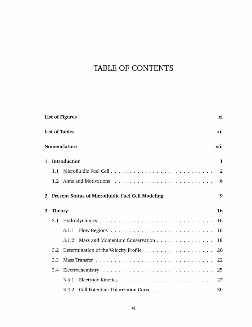
TABLE OF CONTENTS

List of Figures xi

List of Tables xii

Nomenclature xiii

1 Introduction 1

1.1 Microfluidic Fuel Cell . . . . . . . . . . . . . . . . . . . . . . . . . . . 2

1.2 Aims and Motivations . . . . . . . . . . . . . . . . . . . . . . . . . . 6

2 Present Status of Microfluidic Fuel Cell Modeling 9

3 Theory 16

3.1 Hydrodynamics . . . . . . . . . . . . . . . . . . . . . . . . . . . . . . 16

3.1.1 Flow Regions . . . . . . . . . . . . . . . . . . . . . . . . . . . 16

3.1.2 Mass and Momentum Conservation . . . . . . . . . . . . . . . 18

3.2 Determination of the Velocity Profile . . . . . . . . . . . . . . . . . . 20

3.3 Mass Transfer . . . . . . . . . . . . . . . . . . . . . . . . . . . . . . . 22

3.4 Electrochemistry . . . . . . . . . . . . . . . . . . . . . . . . . . . . . 25

3.4.1 Electrode Kinetics . . . . . . . . . . . . . . . . . . . . . . . . 27

3.4.2 Cell Potential: Polarization Curve . . . . . . . . . . . . . . . . 30

vi

3.4.3 Voltage Losses . . . . . . . . . . . . . . . . . . . . . . . . . . 32

4 Modeling 34

4.1 Layout of Model Development . . . . . . . . . . . . . . . . . . . . . . 35

4.2 Model Description . . . . . . . . . . . . . . . . . . . . . . . . . . . . 35

4.3 Constants and Variables . . . . . . . . . . . . . . . . . . . . . . . . . 36

4.4 Test Modeling: Cottrell Experiment . . . . . . . . . . . . . . . . . . . 37

4.4.1 Introduction . . . . . . . . . . . . . . . . . . . . . . . . . . . 37

4.4.2 Statement of the Problem . . . . . . . . . . . . . . . . . . . . 38

4.4.3 Model Description . . . . . . . . . . . . . . . . . . . . . . . . 39

4.4.4 Results . . . . . . . . . . . . . . . . . . . . . . . . . . . . . . . 42

4.5 2-Dimensional Model . . . . . . . . . . . . . . . . . . . . . . . . . . . 45

4.5.1 Model Introduction . . . . . . . . . . . . . . . . . . . . . . . . 45

4.5.2 Model Definition . . . . . . . . . . . . . . . . . . . . . . . . . 45

4.5.3 Charge Balance . . . . . . . . . . . . . . . . . . . . . . . . . . 48

4.5.4 Hydrodynamic and Mass Transport . . . . . . . . . . . . . . . 50

4.5.5 Results . . . . . . . . . . . . . . . . . . . . . . . . . . . . . . . 52

4.6 3-Dimensional Model . . . . . . . . . . . . . . . . . . . . . . . . . . . 56

4.6.1 Model Introduction . . . . . . . . . . . . . . . . . . . . . . . . 56

4.6.2 Model Definition . . . . . . . . . . . . . . . . . . . . . . . . . 57

4.6.3 Charge Balance . . . . . . . . . . . . . . . . . . . . . . . . . . 60

4.6.4 Hydrodynamic and Mass Transport . . . . . . . . . . . . . . . 61

4.6.5 Mesh and Validation . . . . . . . . . . . . . . . . . . . . . . . 63

4.6.6 Results . . . . . . . . . . . . . . . . . . . . . . . . . . . . . . . 67

5 Conclusions and Future Directions 76

5.1 Conclusion and Contribution . . . . . . . . . . . . . . . . . . . . . . 76

5.2 Future Directions . . . . . . . . . . . . . . . . . . . . . . . . . . . . . 79

vii

References 81

Index 84

viii

LIST OF FIGURES

1.1 PEMFC theoretical design . . . . . . . . . . . . . . . . . . . . . . . . 2

1.2 Microfluidic Fuel Cells theoretical design . . . . . . . . . . . . . . . . 5

3.1 Establishment of a Poiseuille profile for a laminar flow in a microchannel.(1) 17

3.2 The definition of rectangular channel cross section . . . . . . . . . . 20

3.3 (a) Contour lines for the velocity field vx(y, z) for the Poiseuille-flow

problem in a rectangular channel. The contour lines are shown in

steps of 10% of the maximal valuevx(0, h/2). (b) A plot of vx(y, h/2)

along the long centerline parallel to ey. (c) A plot of vx(0, z) along the

short centerline parallel to ez.(1) . . . . . . . . . . . . . . . . . . . . 21

3.4 2-Dimensional Velocity Profile in Rectangular Cross Section Channel. 22

3.5 3-Dimensional Velocity Profile in Rectangular Cross Section Channel. 22

3.6 Overpotential on the electrodes . . . . . . . . . . . . . . . . . . . . . 27

3.7 Voltage losses in the fuel cell (2) . . . . . . . . . . . . . . . . . . . . 31

4.1 Heterogeneous kinetics and diffusion . . . . . . . . . . . . . . . . . . 38

4.2 Model domain with boundaries corresponding to the anode, cathode,

and horizontal insulate walls. . . . . . . . . . . . . . . . . . . . . . . 40

4.3 Oxidant concentration (mole/m3), current density streamlines in the

tube after 100 seconds of operation. . . . . . . . . . . . . . . . . . . 42

ix

4.4 Reductant concentration (mole/m3), current density streamlines in

the tube after 100 seconds of operation. . . . . . . . . . . . . . . . . 43

4.5 Concentration profile changing with time. Analytical solution from

error function is presented in red color, and numerical solution from

modeling is presented in purple color. . . . . . . . . . . . . . . . . . 44

4.6 2-D Model geometry with subdomain and boundary labels . . . . . . 46

4.7 HCOOH concentration distribution in 2D model . . . . . . . . . . . . 53

4.8 Oxygen concentration distribution in 2D model . . . . . . . . . . . . 53

4.9 HCOOH concentration distribution of the cross section on 10mm

from the outlets . . . . . . . . . . . . . . . . . . . . . . . . . . . . . . 54

4.10 Oxygen concentration distribution of the cross section on 10mm from

the outlets . . . . . . . . . . . . . . . . . . . . . . . . . . . . . . . . . 54

4.11 Current density along the anode . . . . . . . . . . . . . . . . . . . . . 55

4.12 Current density along the cathode . . . . . . . . . . . . . . . . . . . . 55

4.13 Procedure of building final 3D microfluidic fuel cell model . . . . . . 57

4.14 3D Model geometry . . . . . . . . . . . . . . . . . . . . . . . . . . . . 58

4.15 3D Model cross section profile . . . . . . . . . . . . . . . . . . . . . . 58

4.16 3D Model outlets part view . . . . . . . . . . . . . . . . . . . . . . . 59

4.17 Solution convergence from different meshes . . . . . . . . . . . . . . 64

4.18 Verification of the proposed model against the results reported by

Chang et al. (3) for a numerical model results . . . . . . . . . . . . . 65

4.19 T- and Y-shaped microchannel designs . . . . . . . . . . . . . . . . . 66

4.20 Comparison of cell performance between Y- and T-shaped channel

design . . . . . . . . . . . . . . . . . . . . . . . . . . . . . . . . . . . 66

4.21 3D Model velocity profile . . . . . . . . . . . . . . . . . . . . . . . . 67

4.22 3D Model HCOOH concentration distribution . . . . . . . . . . . . . 68

4.23 3D Model O2 concentration distribution . . . . . . . . . . . . . . . . 69

x

4.24 The current and power density curves for three assigned inlet pressure. 70

4.25 The current and power density curves for three assigned inlet pressure. 71

4.26 The current and power density curves for three assigned convergence

angle. . . . . . . . . . . . . . . . . . . . . . . . . . . . . . . . . . . . 72

4.27 The current and power density curves for three assigned inlet pressure. 73

4.28 The current and power density curves for three assigned concentra-

tions of oxygen. . . . . . . . . . . . . . . . . . . . . . . . . . . . . . . 74

4.29 The current and power density curves for three assigned porosities

of cathode catalyst layer. . . . . . . . . . . . . . . . . . . . . . . . . . 75

xi

LIST OF TABLES

4.1 Operating and physical conditions . . . . . . . . . . . . . . . . . . . 37

4.2 Operating and physical conditions for 2-Dimensional microfluidic fuel

cell . . . . . . . . . . . . . . . . . . . . . . . . . . . . . . . . . . . . . 47

4.3 Operating and physical conditions for 3-Dimensional microfluidic fuel

cell . . . . . . . . . . . . . . . . . . . . . . . . . . . . . . . . . . . . . 60

4.4 Different MESHs and corresponding NOFS, NE, and SOLUTION TIME 64

xii

Chapter 1INTRODUCTION

It is a more and more accepted sense now that fuel cells are one of the most

fascinating and interesting aspects of today’s technology. The interest in

fuel cells has been intensified during the past decade due to the fact that

the use of fossil fuels for generating power has resulted in several negative

consequences, including severe pollutions, exhaustive exploitation of the global re-

sources, and imbalance in political power caused by uneven distribution of natural

resources. Such problems underline the need for a new power source-fuel cell,

which is energy efficient, environmental friendly and renewable. Fuel cells are now

closer to commercialization than ever, and they have the potential in helping to ful-

fill the world’s demand for power and at the same time reach the requirement and

the expectation on environmental protection. Despite all the advantages enumer-

ated above, this field is still under development. Under the influence of booming

MEMS technology, the fabrication of microscale devices has experienced a consider-

able growth. As a result, the demands for energy resources used in portable devices

are under continual pressure to decrease both consumed power and weight. Both

1

demands can be satisfied well by miniaturized power resource, such as microfluidic

fuel cell.

1.1 Microfluidic Fuel Cell

A fuel cell is an electrochemical conversion device. It produces electricity with

fuel (on the anode side) and an oxidant (on the cathode side), in the presence

of an electrolyte. The reactants flow into the cell, and the reaction products flow

out of it, while the electrolyte remains within it. Fuel cells can operate virtually

continuously as long as the necessary flows are maintained. Since it is effective and

environmentally friendly, it is getting an increasingly wide popularity. Presently,

fuel cells have been used in automobiles and space shuttle, even for cell phones

and lap tops.

Proton exchange membrane(PEM) fuel cell, also known as polymer electrolyte

membrane fuel cell (PEMFC),are suitable for various applications such as transport

applications, and both stationary and portable fuel cell applications.

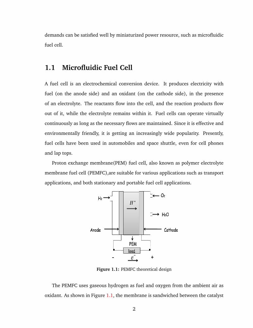
Figure 1.1: PEMFC theoretical design

The PEMFC uses gaseous hydrogen as fuel and oxygen from the ambient air as

oxidant. As shown in Figure 1.1, the membrane is sandwiched between the catalyst

2

layers, gas-diffusion electrodes, and bipolar plates for the anode and cathode. From

the two bipolar plates(containing fuel-left and oxidant-right flow channels), the re-

actants diffuse through the gas-diffusion electrodes and react at the catalyst layers,

the protons released at the anode reaction travel through the ion conducting mem-

brane, and the electrons released follow an external path. The redox reactions at

the anode and cathode drive the operation of the fuel cell by producing an electric

potential and a current through an applied load.

Nevertheless, the PEMFC has problems associated with its operation. High tem-

peratures can improve the efficiency of fuel cells due to fast kinetics, but on the

other hand tend to dry out the PEM, reducing the effectiveness of proton con-

duction. Thus water management becomes crucial since the PEM has to be kept

hydrated at all times in order to facilitate the transport of protons. Another signif-

icant problem for PEMFC is fuel crossover through the membrane, which results in

a mixed potential at the cathode and thereby lowers the cell performance. Despite

extensive efforts, these problems still remain major obstacles preventing PEMFC

from wide-scale portable applications (4).

Based on those problems mentioned above, a new type of fuel cell comes out to

overcome these issues – the Microfluidic Fuel Cell defined as a fuel cell with fluid

transport, reaction sites and electrode structures all confined to a microfluidic chan-

nel. This type of fuel cell operates without a physical barrier, such as a membrane

which is a costly component in the fuel cell devices, to separate the anode and the

cathode, and can use both metallic and biological catalysts. For a most typical ar-

chitecture of micorfluidic fuel cell, it operates in a co-laminar flow which is able to

delay convective mixing of fuel and oxidant. The laminar flow regime is charac-

terized by high momentum diffusion and low momentum convection which can be

presented by Reynold’s number, usually at a low Reynolds’ number, the two aqueous

streams, one containing the fuel and the other containing the oxidant, will flow in

3

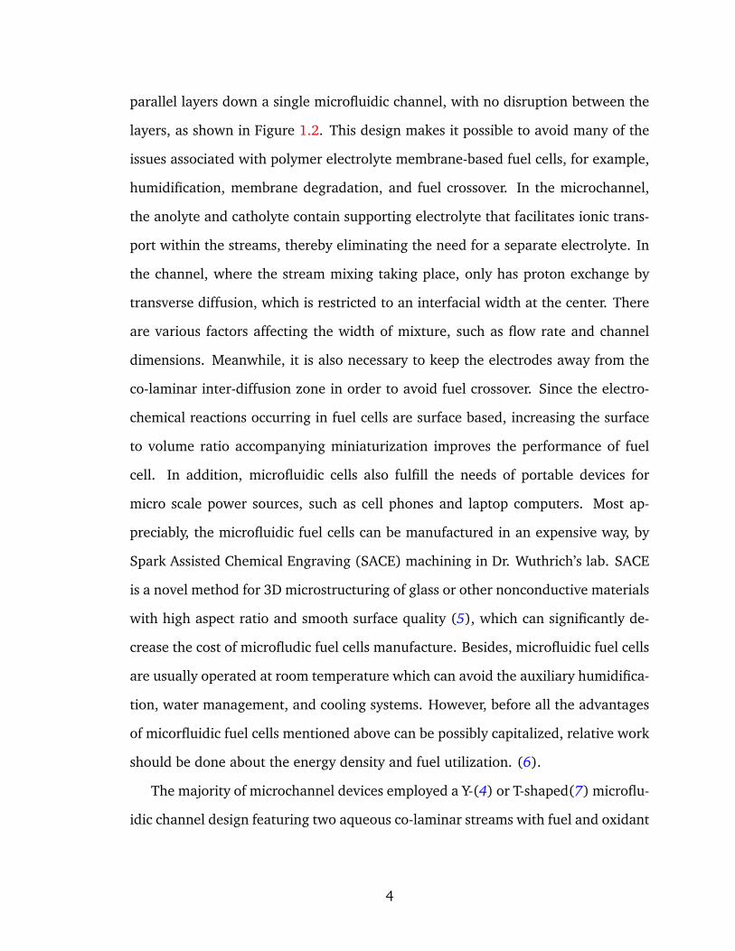
parallel layers down a single microfluidic channel, with no disruption between the

layers, as shown in Figure 1.2. This design makes it possible to avoid many of the

issues associated with polymer electrolyte membrane-based fuel cells, for example,

humidification, membrane degradation, and fuel crossover. In the microchannel,

the anolyte and catholyte contain supporting electrolyte that facilitates ionic trans-

port within the streams, thereby eliminating the need for a separate electrolyte. In

the channel, where the stream mixing taking place, only has proton exchange by

transverse diffusion, which is restricted to an interfacial width at the center. There

are various factors affecting the width of mixture, such as flow rate and channel

dimensions. Meanwhile, it is also necessary to keep the electrodes away from the

co-laminar inter-diffusion zone in order to avoid fuel crossover. Since the electro-

chemical reactions occurring in fuel cells are surface based, increasing the surface

to volume ratio accompanying miniaturization improves the performance of fuel

cell. In addition, microfluidic cells also fulfill the needs of portable devices for

micro scale power sources, such as cell phones and laptop computers. Most ap-

preciably, the microfluidic fuel cells can be manufactured in an expensive way, by

Spark Assisted Chemical Engraving (SACE) machining in Dr. Wuthrich’s lab. SACE

is a novel method for 3D microstructuring of glass or other nonconductive materials

with high aspect ratio and smooth surface quality (5), which can significantly de-

crease the cost of microfludic fuel cells manufacture. Besides, microfluidic fuel cells

are usually operated at room temperature which can avoid the auxiliary humidifica-

tion, water management, and cooling systems. However, before all the advantages

of micorfluidic fuel cells mentioned above can be possibly capitalized, relative work

should be done about the energy density and fuel utilization. (6).

The majority of microchannel devices employed a Y-(4) or T-shaped(7) microflu-

idic channel design featuring two aqueous co-laminar streams with fuel and oxidant

4

Figure 1.2: Microfluidic Fuel Cells theoretical design

dissolving in a supporting electrolyte and electrodes on the opposite channel walls

parallel to the inter-diffusion zone.

The two physicochemical phenomena that govern the chemical conversion and

the energy and mass transport phenomena in these laminar flow-based fuel cells

occurring at the same time are examined. They are(i) depletion of reactants at

the electrode walls and (ii) diffusion across the mutual liquid-liquid interface. An

external reference electrode has also been introduced, enabling separate and si-

multaneous assessment of the individual performance of the anode and cathode

in a single experiment. This method for direct evaluation of the anode and cath-

ode performance through the use of an external reference electrode provides an

excellent tool for system analysis.

A limiting factor in the operation of the laminar flow-based microfluidic fuel cell

is the low solubility of oxygen in solution which causes significant mass transfer

limitations during higher current operation. In addition, depletion boundary layers

form as a result of fuel and oxidant reacting on the anode and cathode respectively,

5

causing mass transfer limitations as well. The choice of catalyst, fuel and oxidant is

therefore crucial for performance optimization.

1.2 Aims and Motivations

In this thesis, the fundamentals behind microfluidic fuel cell technology will be

described first. The following part will present the development of microfluidic

fuel cells to date. Series consideration will be given to choice of reactants, elec-

trochemical reactions, transport characteristics and, particularly here, cell architec-

tures. Microfluidic fuel cell architecture is an area that has seen particularly rapid

development, as discussed by Bazylak et al. (7). In oder to solve those problems

mentioned previously, on the one hand, a mathematical model has been built to

study the single and linked simultaneous reactions occurring at the cathode elec-

trode of the microfluidic fuel cell. The reason for focusing only on the cathode-side

reactions originates from a report (4) which mention that the entire current density

cannot increase significantly with the fuel concentration but can be limited obvi-

ously by the low oxidant concentration. The experiments(4) showed that the cell’s

performance was cathode limited. Accordingly, this thesis has been concentrated

on developing three-dimensional half cell models for studying the cases of single

reaction and linked simultaneous reactions occurring at the cathode.

It begins with the governing equations for the steady incompressible parallel

flows. Mass transport equations and Navier-Stokes equation have been solved as

well; On the other hand, by using COMSOL® which is a multiphysic software able to

combine several phenomena based on polarization curves, and a numerical model

has been developed to determine the effect of the channel geometry on cell per-

formance. The Butler-Volmer model is used to determine the reaction rates at the

electrodes. Two Conductive Media DC modules representing electronic transport

6

in the external circle and ionic transport in the internal circle respectively are used

to model the electric fields within the fuel cell. The concentration distributions of

the reactant species and velocity distributions of the flow are obtained by using

the Incompressible Navier-Stokes and Convection and Diffusion modules. Solving

these equations together predicts the current density for the given cell voltage val-

ues. The results demonstrate the cell voltage losses due to activation, ohmic and

concentration overpotentials. By changing the model geometry to minimize these

overpotentials, this computational tool plays a critical role in the design of high

power density microfluidic fuel cells without lengthy and expensive physical tests.

The first part of this thesis is a numerical analysis of a microfluidic fuel cell con-

sisting of a Y-shaped microchannel in which fuel and oxidant flow in parallel in the

laminar regime. The system considered here is based on the design of Choban et al.

and a theoretical model is deduced to demonstrate flow kinetics, species transport,

and electrochemical reactions at the electrodes with appropriate boundary condi-

tions. A detailed three-dimensional numerical simulation is performed to give phys-

ical insights for the characteristics of cell performance and provide a helpful guide

to develop the computational model for the next step.

After built up the theoretical model, based on the model and the results gener-

ated, a numerical analysis of a microfluidic fuel cell will be conducted. Computa-

tional fluid dynamics (CFD) is an essential tool for numerical analysis on microflu-

idic process. In contrast to macroscale fluid mechanics where there are challenges

in modeling turbulence, the main challenges in CFD modeling of microflows lie in

the application of appropriate boundary conditions and in modeling species trans-

port. A computational model was employed by COMSOL® to analyze a Y-shaped

microfluidic fuel cell with side-by-side streaming. The multidimensional nature

of the flow requires a 3D solution using a computational fluid dynamics frame-

work coupled flow, species transport and electrochemical models for both anode

7

and cathode. The model accounts fully for three-dimensional convective transport

in conjunction with anodic and cathodic reaction kinetics. Appropriate boundary

conditions for the CFD modeling of this system are developed and applied in the

numerical model. The results provide insight into the running parameter, and both

microchannel and electrode geometries required to achieve significantly improved

performance. Finally, a numerical simulation will be used to guide the microchan-

nel geometry design process, and electrodes as well.

8

Chapter 2PRESENT STATUS OF MICROFLUIDIC FUEL

CELL MODELING

Fuel cell mathematical modeling is helpful for developers with such ad-

vantages as improvement in their design, enhancement of cost effi-

ciency, as well as both quantitative and qualitative improvement of the

fuel cells generated. The model must be robust and accurate and be

able to provide quick solutions to fuel cell problems. A good model should be able

to predict fuel cell performance under a wide range of operating conditions. Even

a modest fuel cell model will have large predictive power. A few important param-

eters like the cell, fuel and oxidant temperatures, the fuel or oxidant pressures, the

cell potential, and the weight fraction of each reactant must be solved for in the

mathematical model. Instead of conducting several complicated experiments, we

can easily improve the performance of fuel cells by modifying all those important

parameters, as well as changing the design, materials, and achieving optimization.

As soon as we obtain an optimized model, we can start the experiments with the

9

design of model from our simulation and compare the results between the realistic

experiment and the ideal simulation.

There are various commercially available modeling software that have been suc-

cessful in modeling microfluidics processes, such as Fluent® (http://www.fluent.com),

COMSOL® (http://www.comsol.com), CFD-ACE+® from the CFD Research

Corporation® (http://cfdrc.com) and Coventor® (http://www.coventor.com). While

these excellent tools do present the path of least resistance for high-level numerical

analysis, they do in general require the user to acquire some background knowledge

in computational fluid dynamics. In addition, many of these software packages tend

to be focused primarily on simulation of fluid flow and to a lesser extent, species

transport, which as mentioned above does not provide a complete picture of what

is required to engineer a true microfluidic system. The multiphysics capabilities of

COMSOL® , which facilitates the coupling and simultaneous solution of different

fundamental equations along with its point and click interface, make it likely to

be the best candidate of the widely available tools for comprehensive modeling.

Moreover, some research groups have developed their own software besides these

commercial packages, which allow them to be specialized for microfluidic system

development.

Since Choban et al.(8) firstly demonstrated the membraneless fuel cell using

formic acid and oxygen as reactants, this new type of fuel cell also known as

microfluidic fuel cell has been rapidly developed not only by several modeling

cases(3, 7, 9)which are based on numbers of numerical study(10–14), but also

in manufacture field(15–19). They demonstrated that when two streams are flow-

ing in parallel as laminar flow, the streams remain separated, eliminating the need

of membrane. Later, they reported a Y-shaped microfluidic fuel cell system(4), from

those preliminary results, they showed that the fuel cell performance is limited by

the transport of reactants through the concentration boundary layer to the elec-

10

trodes and by the low concentration of oxidant in the cathode stream especially,

better ionic conductivity and new channel designs will be helpful for the improve-

ment in the performance.

Before the demonstration of microfluidic fuel cell by Choban et al.(8), there

were plenty of theoretical research about laminar flow in microchannel, some of

which were involved with fluid mechanics, such as the work done by Ismagilov

et al.(12). It showed that decreasing the channel height while keeping other pa-

rameters constant can decrease not only the Peclet number and make the difference

between the diffusion near the top and bottom walls and in the center in the channel

less significant, but also the extent of the diffusional broadening δ ∼ (DHz/Ua)1/3

(here D is the diffusivity, H is the height of the channel, z is the distance the fluid

flows downstream, and U is the average flow speed.) near the top and bottom walls

in the high-Peclet-number limit; Some of them are involved with electrochemical re-

action. For example, Compton et al.(11) used the backwards implicit (BI) method

to illustrate, under steady-state conditions, of complex electrode reaction mecha-

nisms pertaining coupled homogeneous kinetics and several kinetic species, which

occurred at channel electrodes.

Successively, Lee et al., Phirani and Basu, Chen and Chen, Chen et al.(10, 13,

14, 20) conducted several theoretical studys about microfluidic fuel cell. Chen and

Chen(14) demonstrated a two-dimensional model of microfluidic fuel cell model

by using the spectral method where the eigenvalues are obtained by employing

Galerkin methods. The similarity transform was adopted to separate the concentra-

tions of the oxidant and the intermediate product from their coupled boundary con-

ditions. As is shown by the results, the limiting average current density increases

with the stoichiometry coefficient from electrons in the case of no intermediate

product, yet the maximum electric power is independent of this coefficient. By giv-

ing the concentrations of the oxidant and the intermediate product at the inlet end

11

of the cell, they can obtain a condition with increasing the current density. A opti-

mization research of microfluidic fuel cell had been demonstrated by Lee et al.(10),

it presented theoretical and experimental work to describe the role of flow rate,

microchannel geometry, and location of electrodes within a microfluidic fuel cell

on its performance by using transport principles. The results showed that the per-

formance of fuel cell can be improved when the electrodes used in designing the

device are smaller than a critical length. Besides, Phirani and Basu(13) improved

the fuel utilization by altering the design of the microfluidic fuel cell. In the study,

by introducing a third stream containing sulfuric acid between the fuel and oxidant

stream, it enhanced fuel utilization with an increase from 14.1% to 16%.

On a basis of such theoretical work reported above, some recent modeling works

came out after. Before the modeling work on microfluidic fuel cell, there were

an amount of modeling work on PEM(Proton exchange membrane) fuel cell (21–

24), which are significantly conducive to the micrfluidic fuel cell modeling. Lu

and Reddy(21) combined the experimental and modeling methods to investigate

effects of different factors on the performance of the micro-PEM fuel cell, which

is similar to the micrfluidic fuel cell in most of such factors as contact resistance,

overpotential, and the dimension of the channel. The results showed that species

transport and contact resistance determined the performance of the micro-PEMFC,

hence, the designs of new flow field configurations and assembling modes of micro-

PEMFCs play a crucial role in improving the performance of micro-PEMFCs. These

designs including flow field and assembling mode of micro-PEMFCs are supposed

to improve species transport through microchannels and decrease the contact resis-

tance between gas diffusion layers (GDLs) and current collectors. Mann et al.(22)

demonstrated a theoretical research about the application of Butler-Volmer equa-

tions in the modelling of activation polarization for PEM fuel cells, which is also

applicable to microfluidic fuel cell. For the reason that fuel cell models must be

12

capable of predicting values of the activation polarization which depends on the in-

verse of the electrochemical reaction rate at that electrode interms of Butler-Volmer

equations at both the anode and the cathode, this work summarized the impor-

tant theoretical background, primarily based on the Butler-Volmer equation, which

is common to the development of modelling capability for both anode and cathode

activation polarization terms in any fuel cell. Cheddie and Munroe(23) developed a

three dimensional mathematical model of a PEM fuel cell equipped with a PBI mem-

brane, which involved transport phenomena and polarization effects of the fuel cell.

It predicted that the greatest area of oxygen depletion occur in the cathode cata-

lyst layer just under the ribs. This depletion increases in the direction of flow, and

is more prominent at lower supply gas flow rates. Al-Baghdadi and Al-Janabi(24)

conducted an optimization study of a PEM fuel cell that incorporates the significant

physical processes and the key parameters affecting fuel cell performance by using a

comprehensive three-dimensional, multi-phase, non-isothermal model. This model

featured an algorithm that gives a more realistic reflection of the local activation

overpotentials, which leads to improved prediction of the local current density dis-

tribution. This comprehensive model accounts for the major transport phenomena

in a PEM fuel cell: convective and diffusive heat and mass transfer, electrode kinet-

ics, transport and phase change mechanism of water and potential fields. All these

work can be also applied in microfludic fuel cell modeling.

The first integrated computational study of microfluidic fuel cell based on a

T-shaped channel, a concise eletrochemical model of the key reactions and with ap-

propriate boundary conditions is done by Bazylak et al. (7) in conjunction with

the development of a computational fluid dynamic (CFD) model of this system

that accounts for coupled flow, species transport and reaction kinetics. By comb-

ing hydrodynamic and mass transport model, and reaction model, which represent

mass, momentum and species conservation, and electrochemical kinetics respec-

13

tively, Bazylak et al. built several three-dimensional microfluidic fuel cell models

with different aspect ratios of channel cross section, but adopting the same hy-

draulic diameter. Then it comes to explain why the reactants demonstrate the least

percentage of mixing and the best fuel utilization at the outlet of the fuel cell. The

reason is that the rectangular geometry with a correspondingly high aspect ratio in

the cross-stream direction is the most promising design for the microfluidic fuel cell,

which can effectively decrease the limitation on the performance of the cell caused

by the mass transport of reactants through the concentration boundary layers to the

electrodes. In addition, lowering the inlet velocity and tailoring the electrode shape

design can also enhance fuel utilization.

Yoon et al.(25) presented a microfluidic fuel cell model by Comsol®, and with

the simulation they figured out three methods to improve the performance of pressure-

driven laminar flow-based microreactors by manipulating reaction-depletion bound-

ary layers to overcome mass transfer limitations on the surface of electrodes. In his

work, by coupling the Navier-Stokes equations, the continuity equation, the mass

conservation equation, and within a boundary condition at the electrode, the Butler-

Volmer equation, the model has been built to reduce or even overcome mass transfer

limitations resulting from the presence of a depletion boundary layer on the reac-

tive surface which can significantly improve the performance of microfluidic fuel

cell.

Chang et al. (3) demonstrated a microfluidic fuel cell model containing the flow

kinetics, species transport, and electrochemical reactions within the channel and

the electrodes is developed with appropriate boundary conditions and solved by a

commercial CFD package. Compared to those works that have been done before,

the analysis of the cell’s performance is been focused on modifying some important

physical factors, such as volumetric flow rate, Peclet number, as well as and the

geometric effect of the size of the channel. Results show that a higher Peclet number

14

can help to improve the cell performance by enhancing electrocatalytic activity on

cathode surface since the performance is mainly restricted by the low concentration

of oxygen in cathodic stream, also to prevent the fuel crossover as the result of

the mixing between the fuel and oxidant streams. On the other hand, for a fixed

aspect ratio and volumetric flow rate, a reduction of cross-sectional area will help

to achieve higher performance. Additionally, higher oxygen concentration can help

to improve the performance as well.

15

Chapter 3THEORY

In principle, a microfluidic fuel cell operates like a battery. Unlike a battery, a

microfluidic fuel cell does not run down and does not require recharging. It

will produce energy in the form of electricity and heat as long as fuel is sup-

plied. In this chapter, multiple disciplines which are involved in microfluidic

fuel cell science and technology will be introduced, including microfluidic dynam-

ics, transport phenomena, electrochemistry. Because of the diversity and complexity

of electrochemical and transport phenomena contained in a microfluidic fuel cell,

before we start the microfluidic modeling and simulation, we have to understand

all aspects of the theory.

3.1 Hydrodynamics

3.1.1 Flow Regions

The transport properties of a channel flow depends greatly on the flow region, i.e.

developing or developed, and type, i.e. laminar or turbulent. The hydrodynamic

16

entrance region is where the velocity boundary layer, the pressure gradient, and

wall shear stress are developing together and the entrance length is the distance

to attain their constant conditions i.e. fully developed conditions. However, the

varying asymptotic approaches of the three variables to their constant conditions

make it difficult to decide the entrance length precisely. Although the definition

of the entrance length can be made in several ways depending on the variable

being compared along the channel and the criteria, for engineering purposes, it is

defined customarily as the axial distance from the channel entrance required for the

centerline velocity to reach 99% of the fully developed centerline velocity.

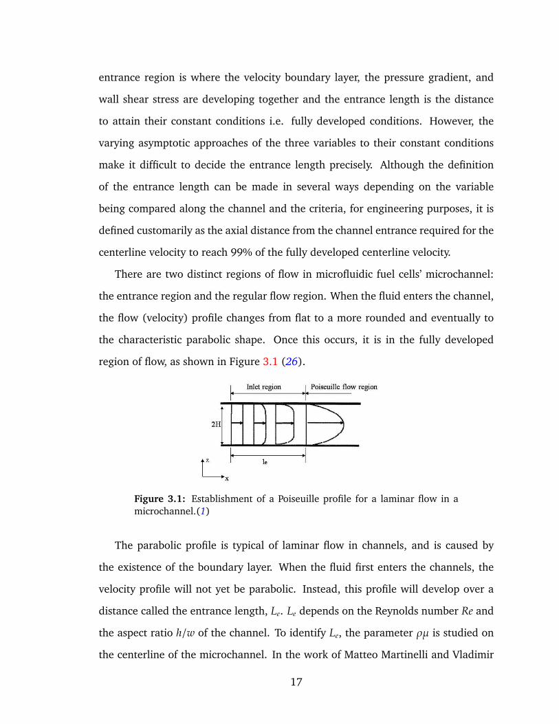
There are two distinct regions of flow in microfluidic fuel cells’ microchannel:

the entrance region and the regular flow region. When the fluid enters the channel,

the flow (velocity) profile changes from flat to a more rounded and eventually to

the characteristic parabolic shape. Once this occurs, it is in the fully developed

region of flow, as shown in Figure 3.1 (26).

Figure 3.1: Establishment of a Poiseuille profile for a laminar flow in amicrochannel.(1)

The parabolic profile is typical of laminar flow in channels, and is caused by

the existence of the boundary layer. When the fluid first enters the channels, the

velocity profile will not yet be parabolic. Instead, this profile will develop over a

distance called the entrance length, Le. Le depends on the Reynolds number Re and

the aspect ratio h/w of the channel. To identify Le, the parameter ρµ is studied on

the centerline of the microchannel. In the work of Matteo Martinelli and Vladimir

17

Viktorov(9), a flow with the parameter ρµ that is 97% of the fully developed value

is considered to be a full-laminar developed flow. Figure 3-2 shows the parameter

ρµ versus the length of the microchannel L with the aspect ratio h/w = 1 and the

Reynolds number Re ranging from 100 to 2100.

The following formula, describing Le, with a maximum error of 4%, is obtained

from numerical results:

Le

h= [−0.129(

hw

)2 + 0.157hw

+ 0.016hw

]Re (3.1)

When the aspect ratio h/w decreases, the fully developed laminar flow will ex-

hibit velocity with a uniform velocity profile. In particular, for h/w < 0.5 velocity

starts to have a uniform profile and for h/w < 0.1 the uniform velocity profile is

90% of the total width of the channel, and flow can be approximated to a 2D flow.

3.1.2 Mass and Momentum Conservation

In a general microfluidic fuel cell device, the Reynolds Number of the flow in the

channel is low (Re < 2300). In a low Reynolds Number, the flow is laminar, by

applying Navier-Stokes equations for momentum conservation in 3-Dimensional in-

compressible Newtonian fluid, we can easily obtain the velocity field. In this work,

the fluid should be treated as a continuum, and this assumption is usually valid in

microscale liquid flows, a reasonable accuracy should be applied into the nanoflu-

idic range. Therefore, after applying aforementioned assumptions, the nonlinear

convective terms of Navier-Stokes equations can be safely neglected at very low

Reynolds numbers, the predictable Stokes flow can be obtained as following:

ρδuδt

= −∇p + µ∇2u + f (3.2)

18

where p represents pressure and f summarizes the body forces per unit volume.

Furthermore, mass conservation for fluid flow obeys the continuity equation:

δρ

δt+ ∇· (ρu) = 0 (3.3)

The incompressible condition is applied since the fluid density is constant. For

a simple geometry such as parallel plates, or a cylindrical tube,equation 3.2 and

equation 3.3 will generate the familiar parabolic pressure-driven velocity profile.

However for our geometry design, which is three dimensional channel with rectan-

gular cross section, needs to have a further discussion is needed.

The characteristic of microfluidic flows offers not only good control over fluid-

fluid interfaces but also significant functionality. When two liquid streams with

similar viscosity and density come into a single microchannel, a parallel co-laminar

flow is formed. In this micrfluidic flow, the mass transport contains three terms:

convection, diffusion, and electromigration. In general, the electromigration term

is neglected since there is sufficient supporting electrolyte, mixing between two co-

laminar streams takes place only by transverse diffusion. The Péclet numbers (Pe =

UDh/D) in microscale devices are usually high, which indicate that the velocity of

mass transfer via stream convective is much higher than transverse diffusion rate,

therefore, the diffusive mixing zone is confined in a thin interfacial width at the

center of the microchannel. In the cross section view, the interdiffusive mixing zone

has an hourglass shape width maximum width (δx) at the channel bottom and top,

and this width is given by the following equation:

δx ∝ (DHz

U)1/3 (3.4)

where D represents the diffusion coefficient, z is the downstream position, and

H is the height of the channel. Equation 3.4 is limited by similar streams density,

19

however, when two liquids have different densities, a gravity-induced reorientation

of the co-laminar liquid-liquid interface can occur(27).

3.2 Determination of the Velocity Profile

As discussed above, in a tube, after the entrance zone, the flow will get fully de-

veloped. Generally, we assume that after the fully developed zone, the flow in the

microchannel is laminar since the Reynolds number is low (Re << 1), after applying

the steady state in the incompressible Stokes equation , neglect the body force(1)

we have:

∇·u = 0 (3.5)

0 = −1ρ∇P + ∇2· (υu) (3.6)

where ρ denotes density (kg·m−1), u the velocity vector (m· s−1), ν denotes kine-

matic viscosity (m2· s−1), and P pressure (Pa).

For equation 3.6, since velocity is a function of y and z, it can be rewritten as:

− ∆PµL

= [δy2 + δz

2]· vx(y, z) (3.7)

For our case, we have a rectangular cross section microchannel as below:

Figure 3.2: The definition of rectangular channel cross section

The Navier-Stokes equation and associated boundary conditions are:

20

−∆P

µL= [δy

2 + δz2]· vx(y, z), for −

1

2w < y <

1

2w, 0 < z < h,

vx(y, z) = 0, for y = ±1

2w, z = 0, z = h,

(3.8)

There is already a solution presented by Bruus (1), which introduces a Fourier

series. The detail for this solution can be found in Theoretical Microfluidics (1).

The solution fn(y) that satisfies the no-slip boundary conditions fn(±12w) = 0 is

fn(y) =4h2∆Pπ3µL

1n3 [1 −

cosh(nπyh )

cosh(nπy

2h )], for n odd, (3.9)

which leads to the velocity field for the Poiseuille flow in a rectangular channel,

vx(y, z) =4h2∆Pπ3µL

∞∑

n,odd

1n3 [1 −

cosh(nπyh )

cosh(nπy

2h )] sin(nπ

zh

). (3.10)

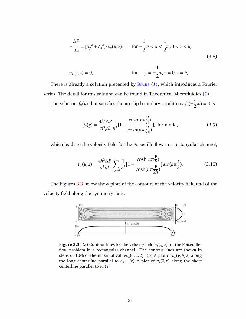
The Figures 3.3 below show plots of the contours of the velocity field and of the

velocity field along the symmetry axes.

Figure 3.3: (a) Contour lines for the velocity field vx(y, z) for the Poiseuille-flow problem in a rectangular channel. The contour lines are shown insteps of 10% of the maximal valuevx(0, h/2). (b) A plot of vx(y, h/2) alongthe long centerline parallel to ey. (c) A plot of vx(0, z) along the shortcenterline parallel to ez.(1)

21

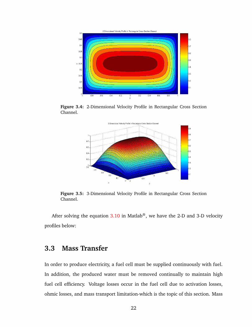
Figure 3.4: 2-Dimensional Velocity Profile in Rectangular Cross SectionChannel.

Figure 3.5: 3-Dimensional Velocity Profile in Rectangular Cross SectionChannel.

After solving the equation 3.10 in Matlab®, we have the 2-D and 3-D velocity

profiles below:

3.3 Mass Transfer

In order to produce electricity, a fuel cell must be supplied continuously with fuel.

In addition, the produced water must be removed continually to maintain high

fuel cell efficiency. Voltage losses occur in the fuel cell due to activation losses,

ohmic losses, and mass transport limitation-which is the topic of this section. Mass

22

transport is the study of the flow of species, and can significantly affect fuel cell per-

formance. Losses due to mass transport are also called "concentration losses," and

can be minimized by optimizing mass transport in the flow field plates, diffusion

layers, and catalyst layers. This section covers both the macro and micro aspects of

mass transport.

After solving the Navier-Stokes equations, we come to the transport equations

which are complicated with chemical processes occurring heterogeneously (i.e. at

the electrode surface; electrochemical reaction) or homogeneously (in the solution;

chemical reaction). In many cases of microfluidics, where the flow velocities are

much smaller than the velocity of pressure waves in the liquid, the fluid can be

regarded as incompressible.

The general transport components are all included in the general Nernst-Planck

equation for the flux Ji of species i, which shows in Equation 3.11 (28)

Ji = −Di∇Ci − ziFRT

DiCi∇φ + Civ, (3.11)

in which Ji is the molar flux per unit area of species i at the given point in space,

Di the species diffusion coefficient, Ci its concentration, zi its charge, F, R and T

have their usual meanings, φ is the potential and v the fluid velocity vector of the

surrounding solution. For solutions containing an excess of supporting electrolyte,

the ionic migration term can be neglected 3.11; we will assume this to be the case

in our study. The velocity vector, v, represents the motion of the solution and is

given in Cartesian coordinates by,

v(x, y, z) = ivx + jvy + kvz, (3.12)

where i, j and k are unit vectors, and vx, vy and vz are the magnitudes of the so-

lution velocities in the x, y and z directions at point (x, y, z). Similarly, in Cartesian

23

coordinates,

∇Ci = gradCi = iδCi

δx+ jδCi

δy+ k

δCi

δz. (3.13)

The variation of Ci with time is given by

δCiδt

= −∇Ji. (3.14)

By combining equation 3.11 and equation 3.13, assuming that migration is ab-

sent and that D j is not a function of x, y and z, we obtain the general convective-

diffusion equation:

δC j

δt= D j∇2C j − v· ∇C j. (3.15)

Note that in the absence of convection (i.e. v = 0), equation 3.15 is reduced

to diffusion equations. Before the convection-diffusion equation can be solved for

the concentration profiles, Ci(x, y, z) and subsequently for the currents from the

concentration gradients at the electrode surface, expressions for the velocity profile,

v(x, y, z), must be obtained in terms of x, y and z.

Previously, we already got the velocity field of the Poiseuille flow in a rectan-

gular cross section microchannel as equation 3.10. When a steady velocity profile

has been attained like Poiseuille flow, the concentrations near the electrode are no

longer functions of time,δCδt , and the steady state convective-diffusion equation

(5), written in terms of Cartesian coordinates, becomes

vx(δCδx

) + vy(δCδy

) + vz(δCδz

) = D[δ2Cδx2 +

δ2Cδy2 +

δ2Cδz2 ]. (3.16)

24

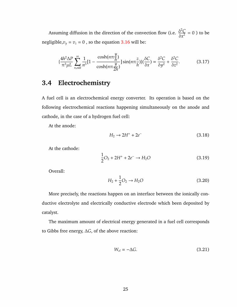
Assuming diffusion in the direction of the convection flow (i.e. δ2Cδx2 = 0 ) to be

negligible,vy = vz = 0 , so the equation 3.16 will be:

4h2∆Pπ3µL

∞∑

n,odd

1n3 [1 −

cosh(nπyh )

cosh(nπy

2h )] sin(nπ

zh

)(δCδx

) =δ2Cδy2 +

δ2Cδz2 . (3.17)

3.4 Electrochemistry

A fuel cell is an electrochemical energy converter. Its operation is based on the

following electrochemical reactions happening simultaneously on the anode and

cathode, in the case of a hydrogen fuel cell:

At the anode:

H2 → 2H+ + 2e− (3.18)

At the cathode:12

O2 + 2H+ + 2e− → H2O (3.19)

Overall:

H2 +12

O2 → H2O (3.20)

More precisely, the reactions happen on an interface between the ionically con-

ductive electrolyte and electrically conductive electrode which been deposited by

catalyst.

The maximum amount of electrical energy generated in a fuel cell corresponds

to Gibbs free energy, ∆G, of the above reaction:

Wel = −∆G. (3.21)

25

The theoretical potential of fuel cell, E, is then:

E =−∆GnF

, (3.22)

where n is the number of electrons involved in the above reaction, and F is

Faraday´s constant (96,485 Coulombs/electron-mol). Since ∆G, n and F are all

known, at 25°C and atmospheric pressure, the theoretical hydrogen oxygen fuel

cell potential can be calculated by:

E =−∆GnF

=237, 3402· 96, 485

Jmol−1

Asmol−1 = 1.23Volts. (3.23)

Assuming that all of the Gibbs free energy can be converted into electrical en-

ergy, the maximum efficiency of a fuel cell that can be achieved (theoretically) is a

ratio between the Gibbs free energy and hydrogen higher heating value, ∆H:

η = ∆G/∆H = 237.34/286.02 = 83% (3.24)

Actual cell potentials are always smaller than the theoretical ones due to in-

evitable losses. Voltage losses in an operational fuel cell are caused by several

factors such as:

• kinetics of the electrochemical reactions (activation polarization),

• internal electrical and ionic resistance,

• difficulties in getting the reactants to reaction sites (mass transport limita-

tions),

• internal (stray) currents,

• crossover of reactants.

26

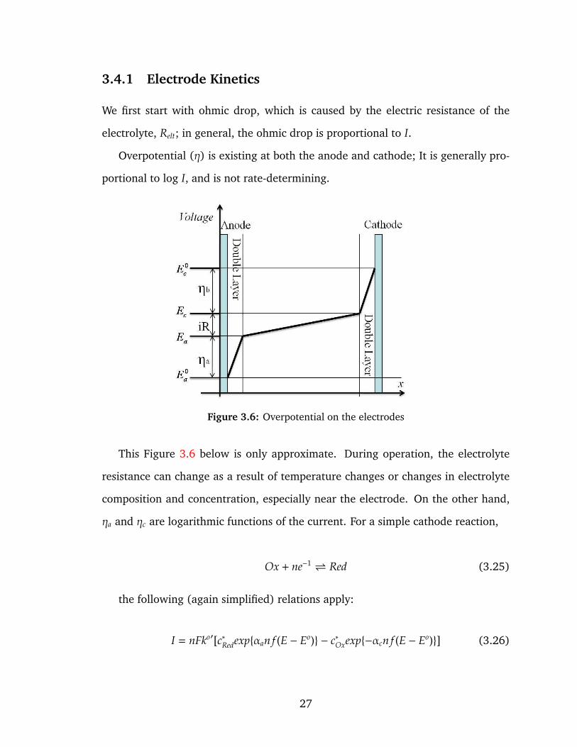
3.4.1 Electrode Kinetics

We first start with ohmic drop, which is caused by the electric resistance of the

electrolyte, Relt; in general, the ohmic drop is proportional to I.

Overpotential (η) is existing at both the anode and cathode; It is generally pro-

portional to log I, and is not rate-determining.

Figure 3.6: Overpotential on the electrodes

This Figure 3.6 below is only approximate. During operation, the electrolyte

resistance can change as a result of temperature changes or changes in electrolyte

composition and concentration, especially near the electrode. On the other hand,

ηa and ηc are logarithmic functions of the current. For a simple cathode reaction,

Ox + ne−1 Red (3.25)

the following (again simplified) relations apply:

I = nFko′[c∗Redexpαan f (E − Eo) − c∗Oxexp−αcn f (E − Eo)] (3.26)

27

or

I = I0[exp(αan fη) − exp(−αcn fη)] (3.27)

with

I0 = nFko′(c∗Ox)αa(c∗Red)αc = Io0(c∗Ox)αa(c∗Red)αc (3.28)

and

η = a + b log |I| (3.29)

with the Tafel slope

b =∂η

∂ log |I| (3.30)

In these equations (2), n, F, E, and Eo have their usual meaning. ko′ is the stan-

dard heterogeneous rate constant (m3· s−2); cRed, cOx represent the concentrations

(mol· dm−3) of the reductant and the oxidant, with the degree symbol representing

the concentration at the phase boundary, and the asterisk the concentration in the

bulk of the solution, respectively.

f =F

RT(3.31)

I0 is the exchange current density in A · m−2; Io0 is standard I0; αa, αc are the

transition coefficients for the anodic and cathodic processes, respectively; αa = 1 −α and αc = α; and η = E − Eeq, i.e., the difference between the actual and the

equilibrium E values (Eeq = E at I = 0); see Figure 3.6.

As soon as the fuel cell reaction starts, the concentrations of reductant and oxi-

dant in the immediate vicinity of the anode, coRed, and the cathode, co

Ox, respectively,

decrease and new reactants are supplied by diffusion. In general, diffusion helps

determine the rate; moreover, the diffusion (and so the current) is governed by

Fick’s law:

28

Ii = nF ·Di(c∗i − coi )/δN, (3.32)

with the subscript i representing species i, Di the diffusion coefficient (m2 · s−1),

and the δN so-called Nernstian diffusion layer.

By calculating, the concentration gradient (c∗i − coi )/δN approaches a maximum

value and so does the current for coi → 0. In that case I → Id, and Id is the diffusion

current. From equation 3.32, it can easily be derived that I ∼ c∗ − co, and so Id ∼ c∗.

Equations 3.26 to 3.28 are valid when the diffusion rate is infinite, which is

rarely true. If diffusion is also rate-determining, then the aforementioned equations

must be transformed to

I = nFko′[coRedexpαan f (E − Eo) − co

Oxexp−αcn f (E − Eo)] (3.33)

I = I0[co

Red

c∗Red

expαan fη − coOx

c∗Ox

exp(−αcn fη)] (3.34)

From a didactic point of view, equation 3.33 and equation 3.34 are easier to

handle: the exchange current (density), I0, is a direct measure of the electrode

reaction rate; a high value means that the reaction proceeds rapidly, or as called in

the electrochemical reversibly.

This is known as the Butler-Volmer equation. Note that the equilibrium potential

at the fuel cell anode is 0V, and the reversible potential at the fuel cell cathode is

1.229V and it does vary with temperature and pressure.

Since the ration proceeds in both directions simultaneously, at equilibrium, the

net current is zero at equilibrium, we still envision balanced faradaic activity that

can be expressed in terms of the exchange current, I0, which is equal in magnitude

to either component current, Ic or Ia.

29

Io = nFkobc

oRedexp[−αan f Er] = nFko

f coOxexp[−αcn f Er] (3.35)

The exchange current density is the measurement of the readiness of the elec-

trode to proceed with the chemical reaction, which depends critically on the nature

of the electrode, besides it is also a function of temperature, catalyst loading, and

catalyst-specific surface area. Therefore, when the exchange current density gets

higher, the electrons get easier to shift, and the surface of electrode gets more ac-

tive.

When the exchange current is very large, the system supplies large currents,

accompanying with insignificant activation overpotential. However, when the ex-

change current is low, no significant current flows can be supplied, in this case, a

large activation overpotential need to be applied. For charge exchange across the

interface, the exchange current can be viewed as a kind of "idle current", and only

a tiny overpotential will be required to obtain a net current that is only a small

fraction of this idle current. If we need for a net current that is higher than the ex-

change current, we have to deliver charge at the required rate by applying a signifi-

cant overpotential. Therefore, exchange current is a measure of any system’s ability

to deliver a net current without a significant energy loss due to activation.(26).

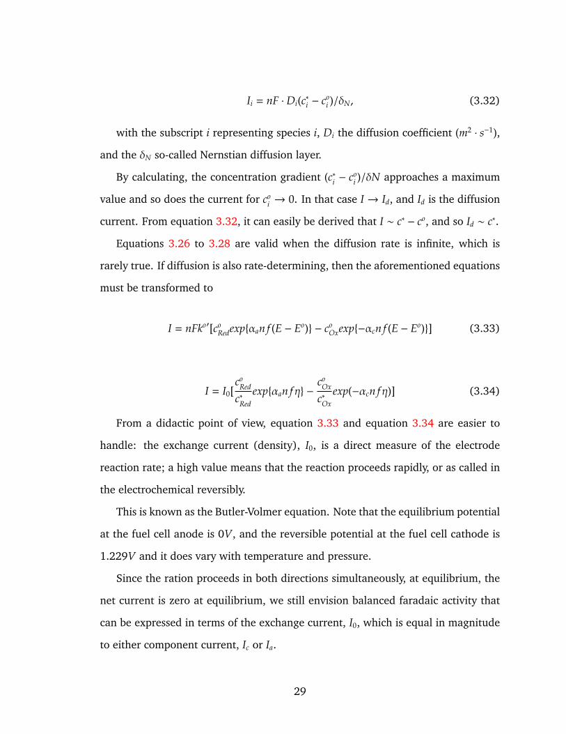
3.4.2 Cell Potential: Polarization Curve

In the electrochemical reaction process of microfluidic fuel cells system, there are

three types of losses as shown in Figure 3.7, and it views the largest losses are the

activation losses at all current density.

Since activation and concentration polarization are taking place at both anode

and cathode, the cell votage can be presented as following:

30

Figure 3.7: Voltage losses in the fuel cell (2)

Vcell = Er − (∆Vact + ∆Vconc)a − (∆Vact + ∆Vconc)c − ∆Vohm (3.36)

Figure 3.6 gives a view of potential distribution in a typical micrfluidic fuel cell

over the cell cross section. At open circuit, when there is no current generated, the

anode is at reference potential which shown as E0a and the cathode is at the potential

corresponding to the reversible potential which shown as E0c at given temperature,

pressure, and oxidant concentration. As soon as the current is being generated, the

cell potential, measured as the difference between cathode and anode solid phase

potentials (solid phase means electrically conductive parts) which shown as Ec−Ea,

drops because of various losses as discussed earlier.

Note that the cell potential is equal to the reversible cell potential (or the equi-

librium potential, Eeq) reduced by the potential losses:

Ecell = Er − Eloss (3.37)

31

where the losses are composed of activation and concentration polarization on

both anode and cathode and of ohmic losses as discussed earlier:

Eloss = ηc + ηa + ∆Vohm = (∆Vact + ∆Vconc)a + (∆Vact + ∆Vconc)c + ∆Vohm (3.38)

The cell potential is equal to the difference between the cathode and the anode

solid state potentials:

Ecell = Ec − Ea (3.39)

where the cathode potential is:

Ec = E0c − ηc = E0

c − (∆Vact + ∆Vconc)c (3.40)

and the anode potential is:

Ea = E0a − ηa = E0

a − (∆Vact + ∆Vconc)a (3.41)

All these potentials may be tracked down in Figure 3.6.

3.4.3 Voltage Losses

As mentioned above, in a microfluidic fuel cell, there are different kinds of voltage

losses caused by several factors, such as kinetics of the electrochemical reactions,

internal electrical and ionic resistance, internal currents and also crossover of re-

actants. Besides, the operating conditions such as temperature, applied load, and

fuel/oxidant flow rates also lead to voltage losses. The three major classifications

of losses that result in the drop from open-circuit voltage are (1) activation polar-

ization, (2) ohmic polarization, and (3) concentration polarization.

32

Activation polarization is a polarization due to charge transfer kinetics of the

electrochemical process involved, and also associated with sluggish electrode kinet-

ics. The higher the exchange current density is, the lower the activation polarization

losses are. These losses take place at both anode and cathode; however, since oxi-

dant reduction is a much lower reaction than hydrogen oxidation, it requires much

higher overpotentials.

The ohmic overpotential appears as the simple product of a resistance and a

current between the anodic and cathodic sites of a fuel cell reaction process, be-

cause of resistance to the flow of ions in the electrolyte and resistance to the flow

of electrons through the electrode. The total internal resistance of fuel cell includes

ionic, electronic, and contact resistance. Electronic resistance is almost negligible,

since the material is used for current collectors can hardly be effective. Ionic and

contact resistances are approximately of the same order of magnitude.

Concentration polarization is the polarization component which caused by con-

centration changes in the environment adjacent to the surface of electrodes. When

a reactant is rapidly consumed, the mass transport of that reactant close to the

surface can become rate controlling. The relationship between the electrochemical

reaction potential changes and partial pressure of the reactants can be given by the

Nernst Equation.

∆V =RTnF

ln(cb

cs) (3.42)

where cb is the bulk concentration of reactant (mol/cm3); cs is the concentration

of reactant at the surface of the catalyst (mol/cm3).

33

Chapter 4MODELING

Computational fluid dynamics (CFD) is an essential tool in the devel-

opment of microfluidic processes. Fuel cell modeling based on CFD

is significantly helpful to improve the design of fuel cell, reduce cost,

and generate more high-efficient fuel cells. It can quickly provide

us a robust and accurate solutions to fuel cell problems, and enables us to predict

fuel cell performance under a wide range of fuel cell operating conditions. The

necessary improvements in fuel cell performance and operation demand better de-

sign, materials, and optimization. These issues can only be addressed if realistic

mathematical process models are available.

COMSOL® is a powerful and interactive environment for modeling and solving

scientific and engineering problems based on partial differential equations. With

some modifications, it can extend conventional models that address one branch of

physics to multiphysics models that simultaneously involve multiple branches of

science and engineering, sequentially, providing a platform to combine fluid and

electrochemical problems in one model.

34

The set of governing equations presented in chapter 3 have been all solved using

COMSOL® Multiphysics 3.5. This chapter is designed to give some background

information on the commercial software and how it has been utilized in order to

solve the problems at hand for this thesis.

4.1 Layout of Model Development

In this chapter, a comprehensive three dimensional microfluidic fuel cell model has

been developed at the end, before that, in order to have an exhaustive understand-

ing on building up such model with COMSOL® Multiphysics, there are a test model

with respect to electrochemical reaction on electrode associate with species diffu-

sion, and an integral two dimensional model of microfluidic fuel cell are presented

respectively, only necessary analysis are given at the end of this two models to val-

idate practicability of COMSOL® modeling on this work. Afterward, for the results

of this final three dimensional microfluidic fuel cell model, a systematic analysis

are presented, with various comparison of some other simulation and experimental

work which have been done.

4.2 Model Description

By understanding the governing equations, we come to the following built-in mod-

ules.

• The convection and diffusion equation module is used to solve for the species

conservation. The species specified are reductant and oxidant. This module

exits in two domains out of four computational domains, and two microchan-

nels. It is set to inactive in the electrodes domain since no reactant specie’s

transport occurs in the electrodes. It is important to choose oxidant as the

35

main species, then it is the reductant, since the entire current density cannot

increase significantly with the fuel concentration but can be limited obviously

by the low oxidant concentration(4).

• The AC/DC Module is employed to compute the solid and electrolyte po-

tentials. Two modules are needed to solve for the potentials, one called

electronic module, represents the solid potential in the electrodes domain

while the other, called ionic module, represents the electrolyte potential in

the microchannel domain. They should work independently, which means

one would be set to inactive when other is active.

• The incompressible Navier-Stokes equation under the chemical engineering

modules used to solve for the momentum conservation and the velocity profile

in the channel. Like the convection and diffusion module, for the reason that

no reactant specie’s transport occurs in the electrodes, it is set to inactive in

the electrodes domain.

4.3 Constants and Variables

There are several ways to input necessary information into COMSOL. The constants

option is used to define those global parameters which are the same for all geome-

tries and subdomains. One can use constants in any physics settings, expressions,

and coupling variables, also one can use them in expressions while postprocessing

the solution. The physical and thermal parameters of this work are defined in Tables

4.1.

The scalar expressions option is used to define expression variables that are valid

on all geometry levels everywhere in the current geometry.

36

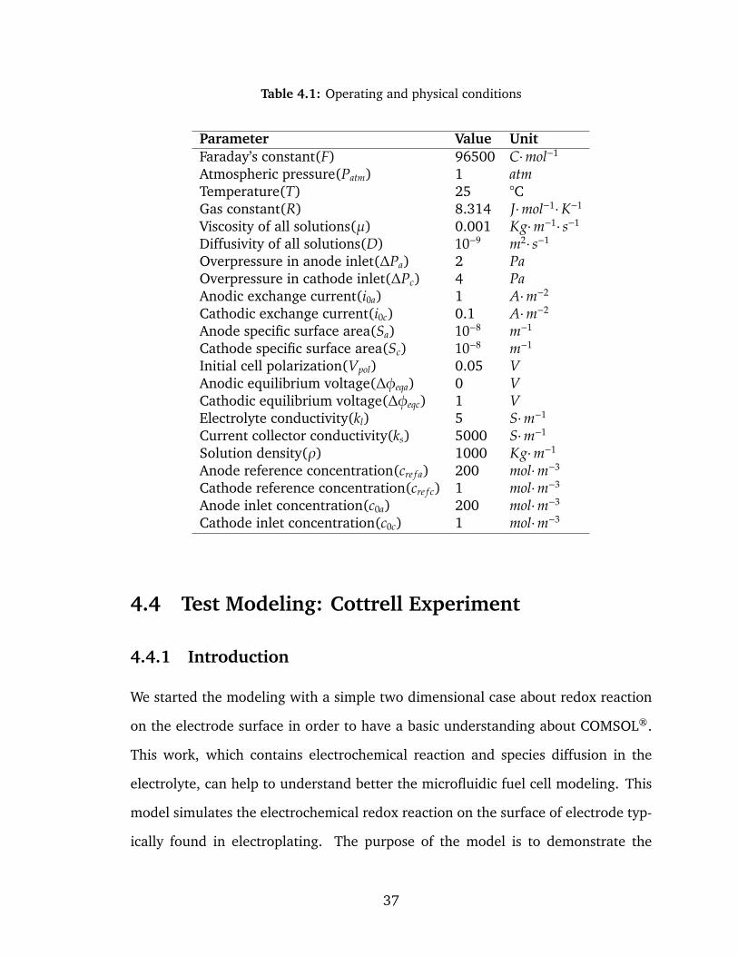
Table 4.1: Operating and physical conditions

Parameter Value UnitFaraday’s constant(F) 96500 C·mol−1

Atmospheric pressure(Patm) 1 atmTemperature(T) 25 °CGas constant(R) 8.314 J·mol−1·K−1

Viscosity of all solutions(µ) 0.001 Kg·m−1· s−1

Diffusivity of all solutions(D) 10−9 m2· s−1

Overpressure in anode inlet(∆Pa) 2 PaOverpressure in cathode inlet(∆Pc) 4 PaAnodic exchange current(i0a) 1 A·m−2

Cathodic exchange current(i0c) 0.1 A·m−2

Anode specific surface area(Sa) 10−8 m−1

Cathode specific surface area(Sc) 10−8 m−1

Initial cell polarization(Vpol) 0.05 VAnodic equilibrium voltage(∆φeqa) 0 VCathodic equilibrium voltage(∆φeqc) 1 VElectrolyte conductivity(kl) 5 S·m−1

Current collector conductivity(ks) 5000 S·m−1

Solution density(ρ) 1000 Kg·m−1

Anode reference concentration(cre f a) 200 mol·m−3

Cathode reference concentration(cre f c) 1 mol·m−3

Anode inlet concentration(c0a) 200 mol·m−3

Cathode inlet concentration(c0c) 1 mol·m−3

4.4 Test Modeling: Cottrell Experiment

4.4.1 Introduction

We started the modeling with a simple two dimensional case about redox reaction

on the electrode surface in order to have a basic understanding about COMSOL®.

This work, which contains electrochemical reaction and species diffusion in the

electrolyte, can help to understand better the microfluidic fuel cell modeling. This

model simulates the electrochemical redox reaction on the surface of electrode typ-

ically found in electroplating. The purpose of the model is to demonstrate the

37

coupling transient diffusion module with conductive media DC and to investigate

the reactant concentration distribution in terms of time-dependent factor, diffusion

layer, and voltammograms.

4.4.2 Statement of the Problem

We consider our simple redox reaction as:

Red⇔ Ox + ne− (4.1)

in the condition of applying a constant potential voltage on the two sides of elec-

trode as 0.2V. The electrochemical reaction takes place on the surface of the elec-

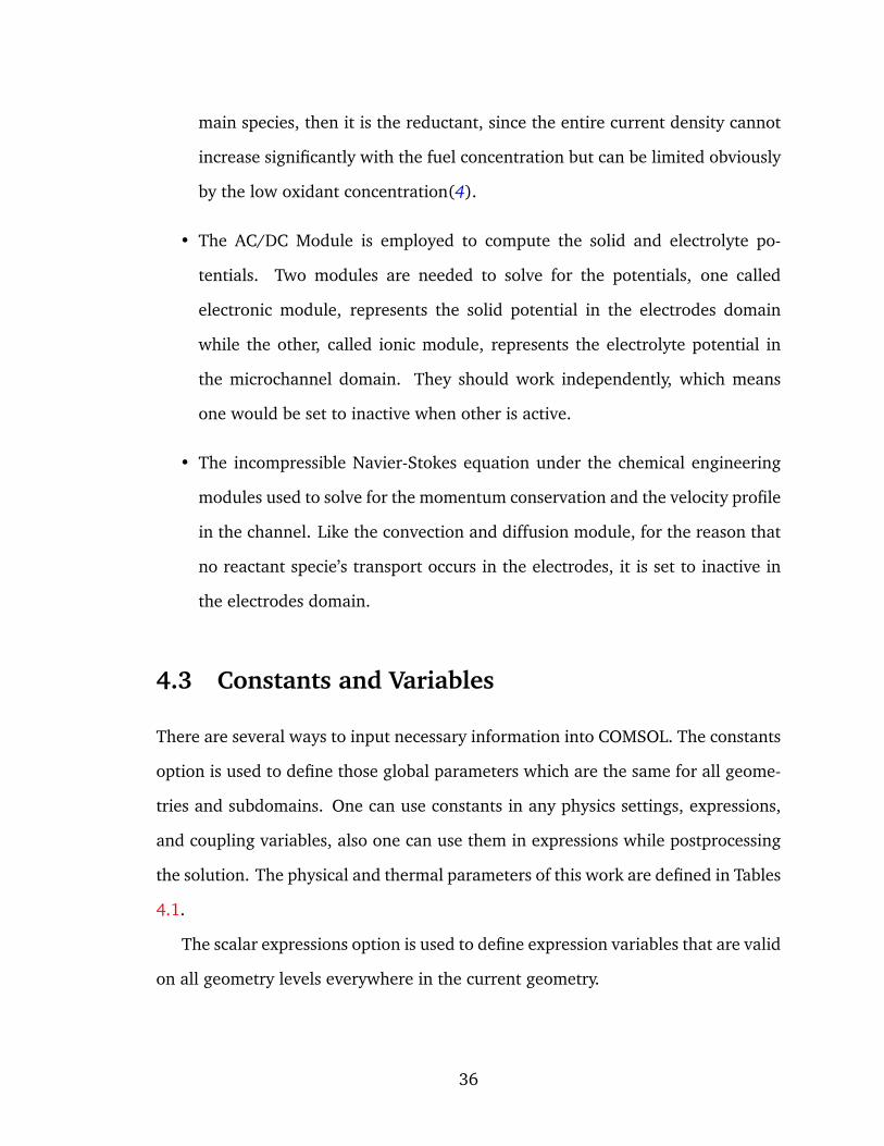
trode (x=0). The reactants first have to diffuse through the electrolyte in order to

be able to proceed to the electron transfer. The situation is controlled by diffusion

and heterogeneous kinetics shown in Figure 4.1.

Figure 4.1: Heterogeneous kinetics and diffusion

The diffusion in the electrolyte is described by Fick’s laws:

38

δcox

δt= Dox

δ2cox

δx2

δcred

δt= Dred

δ2cred

δx2

(4.2)

At the electrode surface one has (anodic current is positive)

j = −nFDoxδcox

δx|x=0 = nFDred

δcred

δx|x=0 (4.3)

As initial and boundary conditions we have:

t = o, x ≥ 0 cred = c0red

t ≥ o, x→ 0 cred = c0red

(4.4)

and if we assume that no oxidant is present at the beginning of the experiment:

t = o, x ≥ 0 cox = 0

t ≥ o, x→ 0 cox = 0

(4.5)

The partial differential equation 4.2 being of second order, we need a second

boundary condtion. This second condition depends on the type of reaction being

considered and is derived from equation 4.3.

4.4.3 Model Description

The physical domain of the model is a 2-dimensional channel through which the

flow is happening is independent on z position, it might be tempting to consider

the flow to be two-dimensional. The model geometry is depicted in Figure 4.2.

39

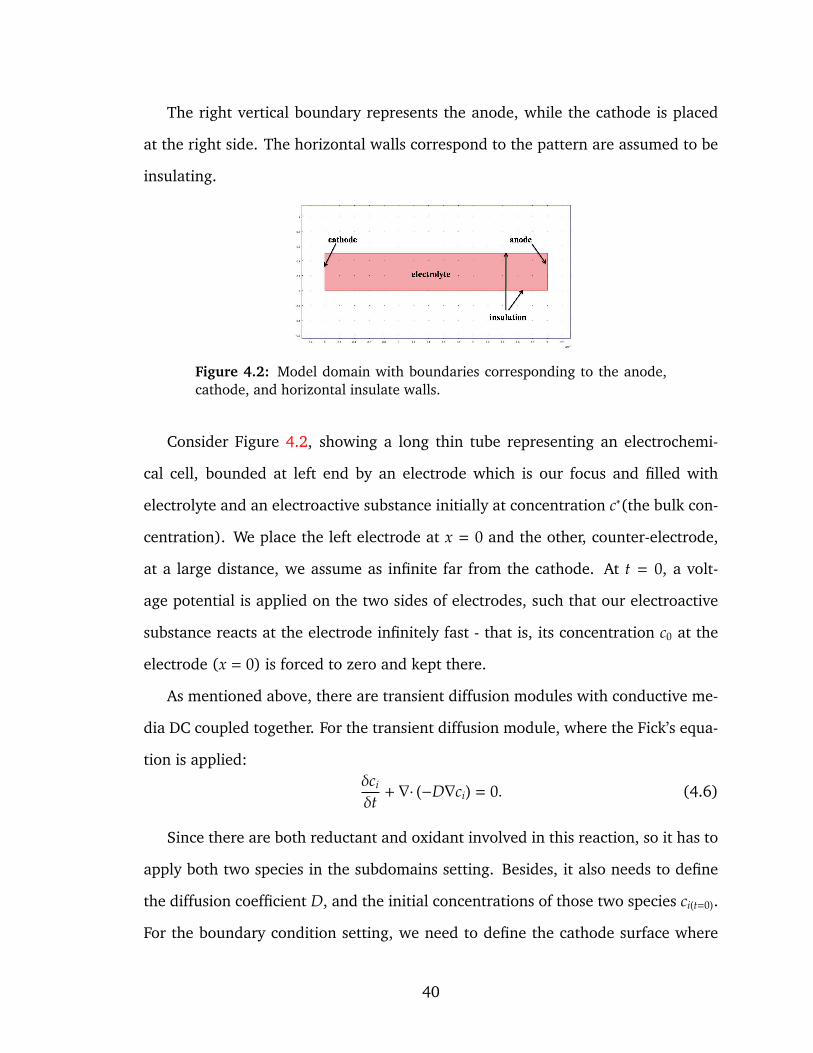
The right vertical boundary represents the anode, while the cathode is placed

at the right side. The horizontal walls correspond to the pattern are assumed to be

insulating.

Figure 4.2: Model domain with boundaries corresponding to the anode,cathode, and horizontal insulate walls.

Consider Figure 4.2, showing a long thin tube representing an electrochemi-

cal cell, bounded at left end by an electrode which is our focus and filled with

electrolyte and an electroactive substance initially at concentration c∗(the bulk con-

centration). We place the left electrode at x = 0 and the other, counter-electrode,

at a large distance, we assume as infinite far from the cathode. At t = 0, a volt-

age potential is applied on the two sides of electrodes, such that our electroactive

substance reacts at the electrode infinitely fast - that is, its concentration c0 at the

electrode (x = 0) is forced to zero and kept there.

As mentioned above, there are transient diffusion modules with conductive me-

dia DC coupled together. For the transient diffusion module, where the Fick’s equa-

tion is applied:δci

δt+ ∇· (−D∇ci) = 0. (4.6)

Since there are both reductant and oxidant involved in this reaction, so it has to

apply both two species in the subdomains setting. Besides, it also needs to define

the diffusion coefficient D, and the initial concentrations of those two species ci(t=0).

For the boundary condition setting, we need to define the cathode surface where

40

the reaction occurred as two fluxes from equation 4.3. The anode side is assumed

to be infinitely far away from the cathode, i.e, the concentration of the reactant on

the surface is fixed as the bulk concentration while the concentration of the product

is zero.

A Conductive Media DC application module describes the potential distributions

in the subdomain using the following equations:

∇· (−kl,e f f∇φl) = 0. (4.7)

Here kl,e f f is the effective electronic conductivity (S/m) of the electrolyte. The

potential (V) in the electrolyte phases is denoted by φl. This models the active layer

of the two electrodes as boundaries. It means that the charge-transfer current den-

sity can be generally described by using the Butler-Volmer electrochemical kinetic

expressions as in Equation 4.8, as a boundary condition on the surface of cathode.

ic = i0

(cred

c0red

exp0.5Fη

RT− cox

c0ox

exp−0.5Fη

RT

)(4.8)

where i0 is the exchange current density (A/m2), cred and c0red are the concentra-

tion on the surface of electrode and bulk concentration of reductant respectively

(mol/m3), cox and c0ox are the concentration on the surface of electrode and bulk

concentration of oxidant respectively (mol/m3). Furthermore, F is Faraday’s con-

stant (C/mol), R the gas constant (J/(mol·K)), T the temperature (K), and η the

overpotential (V); we assumed a symmetry factor of 0.5.

In addition, on the cathode surface, by applying equation 4.3, we have the

boundary condition below:

− nFDox∂cox

∂x|x=0 = nFDred

∂cred

∂x|x=0 = i0

(cred

c0red

exp0.5Fη

RT− cox

c0ox

exp−0.5Fη

RT

)(4.9)

41

In other words, we have the boundary condition for both reductant and oxidant

on the cathode surface as two fluxes:

∂cox

∂x|x=0 = − i0

nFDox

(cred

c0red

exp0.5Fη

RT− cox

c0ox

exp−0.5Fη

RT

)(4.10)

∂cred

∂x|x=0 =

i0

nFDred

(cred

c0red

exp0.5Fη

RT− cox

c0ox

exp−0.5Fη

RT

)(4.11)

For the anode which is on the other side, we just set the boundary condition as

two fixed concentrations which are the bulk concentration for each of them.

4.4.4 Results

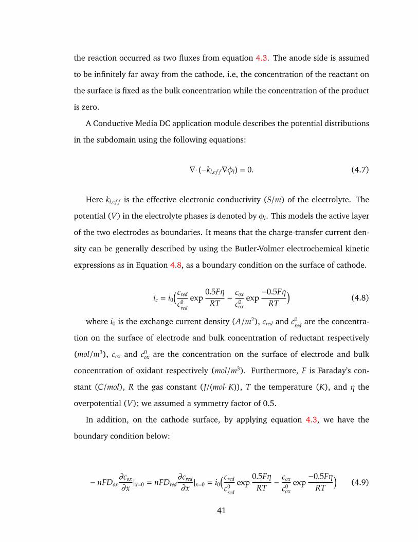
Figure 4.3: Oxidant concentration (mole/m3), current density streamlinesin the tube after 100 seconds of operation.

After meshing with a number of degrees of freedom as 9843, 1568 triangular

elements, we solve the model with time dependent solver for 100 seconds which is

able to give us a full scale set of results.

42

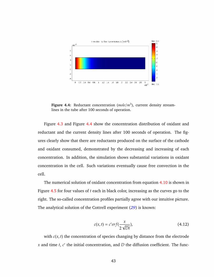
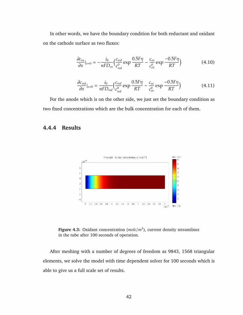
Figure 4.4: Reductant concentration (mole/m3), current density stream-lines in the tube after 100 seconds of operation.

Figure 4.3 and Figure 4.4 show the concentration distribution of oxidant and

reductant and the current density lines after 100 seconds of operation. The fig-

ures clearly show that there are reductants produced on the surface of the cathode

and oxidant consumed, demonstrated by the decreasing and increasing of each

concentration. In addition, the simulation shows substantial variations in oxidant

concentration in the cell. Such variations eventually cause free convection in the

cell.

The numerical solution of oxidant concentration from equation 4.10 is shown in

Figure 4.5 for four values of t each in black color, increasing as the curves go to the

right. The so-called concentration profiles partially agree with our intuitive picture.

The analytical solution of the Cottrell experiment (29) is known:

c(x, t) = c∗er f (x

2√

Dt), (4.12)

with c(x, t) the concentration of species changing by distance from the electrode

x and time t, c∗ the initial concentration, and D the diffusion coefficient. The func-

43

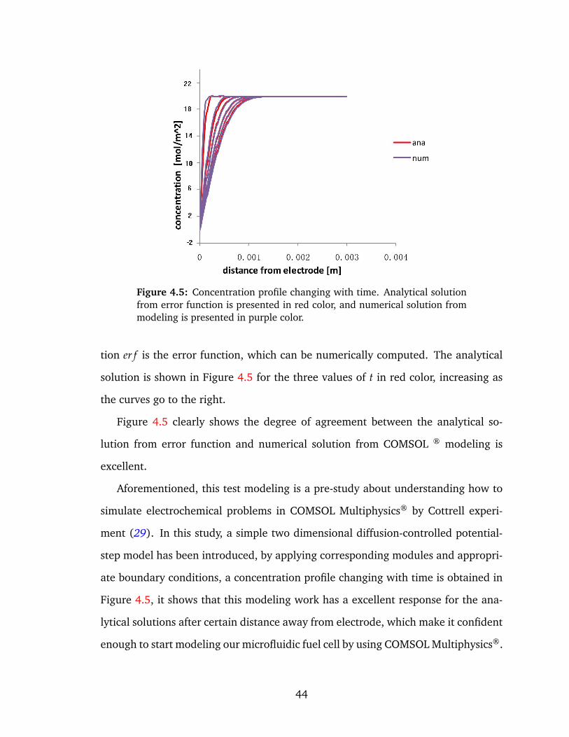
Figure 4.5: Concentration profile changing with time. Analytical solutionfrom error function is presented in red color, and numerical solution frommodeling is presented in purple color.

tion er f is the error function, which can be numerically computed. The analytical

solution is shown in Figure 4.5 for the three values of t in red color, increasing as

the curves go to the right.

Figure 4.5 clearly shows the degree of agreement between the analytical so-

lution from error function and numerical solution from COMSOL ® modeling is

excellent.

Aforementioned, this test modeling is a pre-study about understanding how to

simulate electrochemical problems in COMSOL Multiphysics® by Cottrell experi-

ment (29). In this study, a simple two dimensional diffusion-controlled potential-

step model has been introduced, by applying corresponding modules and appropri-

ate boundary conditions, a concentration profile changing with time is obtained in

Figure 4.5, it shows that this modeling work has a excellent response for the ana-

lytical solutions after certain distance away from electrode, which make it confident

enough to start modeling our microfluidic fuel cell by using COMSOL Multiphysics®.

44

4.5 2-Dimensional Model

4.5.1 Model Introduction

In this section, we build a stationary 2-Dimensional model of a microfluidic fuel

cell based on a training model in COMSOL Multiphysics ® – Proton Exchange Mem-

brane(PEM) Fuel Cell. This PEM fuel cell model uses current balances, mass trans-

port equations (Maxwell-Stefan diffusion for reactant, water and nitrogen gas), and

momentum transport (gas flow) to simulate a PEM fuel cell’s behavior. By applying

microfluidic fuel cell’s condition in the PEM fuel cell model, instead of using Darcy’s

law module and Maxwell-stefan diffusion and convection module, this model em-

ploys incompressible Navier-Stokes module, convection and diffusion module, since

the flow in channel is liquid and there’s no gas diffusion layer. These four modules

help to form a complete fuel cell model. This model simulates the electrochemical

reaction on each electrode by Butler-Volmer equations which make it capable to

couple with convection and diffusion module, additionally, it simulates the flow by

using Navier-Stokes equation. The purpose of this model is to achieve a complete

2-Dimensional microfluidic fuel cell, try to understand the principles of fuel cell

modeling, and prepare for the 3-Dimensional case modeling.

4.5.2 Model Definition

As we can see in Figure 4.7, the modeled section of the fuel cell consists of three

domains: an anode (Ωa), a electrolyte flow domain (Ωe), and a cathode (Ωc). Two

current collectors are located on the top of each electrode. The microchannel has

two inlets and two outlets, which are located on the top and bottom respectively.

For the fuel solution, formic acid has been selected, for the reason that it is a

small organic molecule fed directly into the fuel cell, removing the need for com-

45

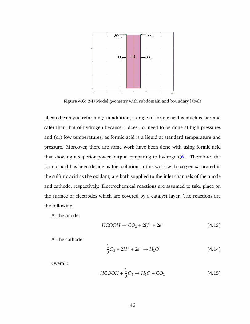
Figure 4.6: 2-D Model geometry with subdomain and boundary labels

plicated catalytic reforming; in addition, storage of formic acid is much easier and

safer than that of hydrogen because it does not need to be done at high pressures

and (or) low temperatures, as formic acid is a liquid at standard temperature and

pressure. Moreover, there are some work have been done with using formic acid

that showing a superior power output comparing to hydrogen(6). Therefore, the

formic acid has been decide as fuel solution in this work with oxygen saturated in

the sulfuric acid as the oxidant, are both supplied to the inlet channels of the anode

and cathode, respectively. Electrochemical reactions are assumed to take place on

the surface of electrodes which are covered by a catalyst layer. The reactions are

the following:

At the anode:

HCOOH→ CO2 + 2H+ + 2e− (4.13)

At the cathode:12

O2 + 2H+ + 2e− → H2O (4.14)

Overall:

HCOOH +12

O2 → H2O + CO2 (4.15)

46

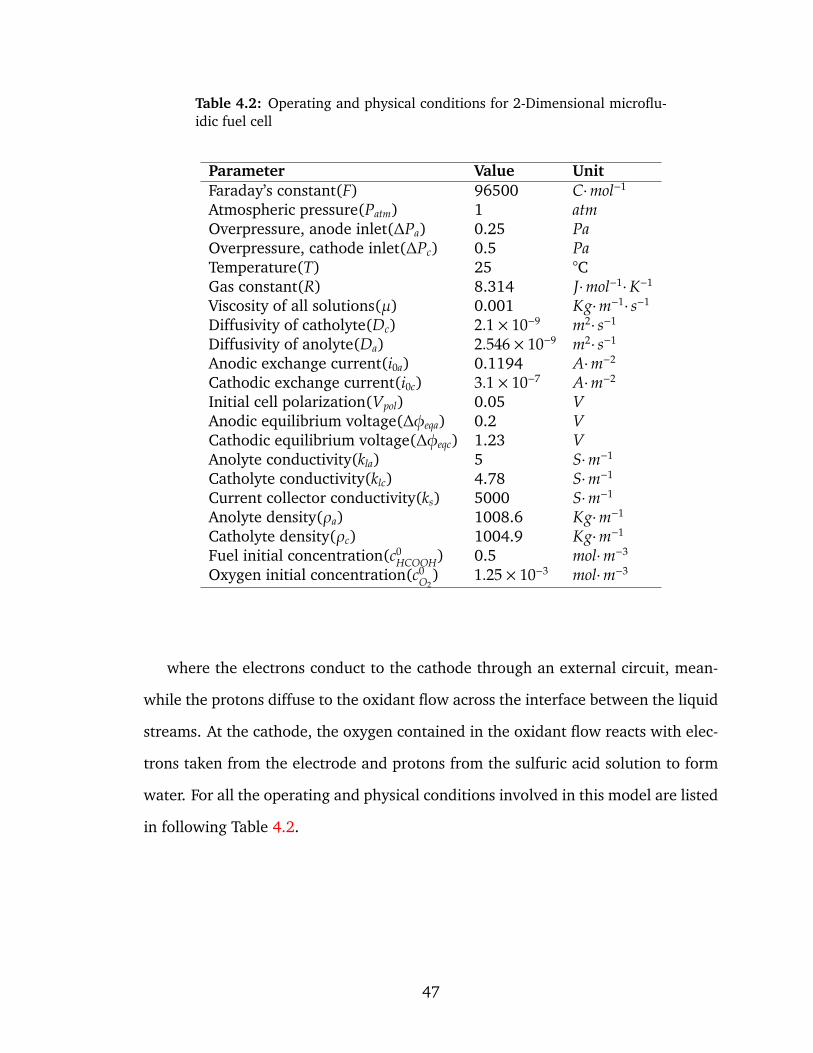
Table 4.2: Operating and physical conditions for 2-Dimensional microflu-idic fuel cell

Parameter Value UnitFaraday’s constant(F) 96500 C·mol−1

Atmospheric pressure(Patm) 1 atmOverpressure, anode inlet(∆Pa) 0.25 PaOverpressure, cathode inlet(∆Pc) 0.5 PaTemperature(T) 25 °CGas constant(R) 8.314 J·mol−1·K−1

Viscosity of all solutions(µ) 0.001 Kg·m−1· s−1

Diffusivity of catholyte(Dc) 2.1 × 10−9 m2· s−1

Diffusivity of anolyte(Da) 2.546 × 10−9 m2· s−1

Anodic exchange current(i0a) 0.1194 A·m−2

Cathodic exchange current(i0c) 3.1 × 10−7 A·m−2

Initial cell polarization(Vpol) 0.05 VAnodic equilibrium voltage(∆φeqa) 0.2 VCathodic equilibrium voltage(∆φeqc) 1.23 VAnolyte conductivity(kla) 5 S·m−1

Catholyte conductivity(klc) 4.78 S·m−1

Current collector conductivity(ks) 5000 S·m−1

Anolyte density(ρa) 1008.6 Kg·m−1

Catholyte density(ρc) 1004.9 Kg·m−1

Fuel initial concentration(c0HCOOH) 0.5 mol·m−3

Oxygen initial concentration(c0O2

) 1.25 × 10−3 mol·m−3

where the electrons conduct to the cathode through an external circuit, mean-

while the protons diffuse to the oxidant flow across the interface between the liquid

streams. At the cathode, the oxygen contained in the oxidant flow reacts with elec-

trons taken from the electrode and protons from the sulfuric acid solution to form

water. For all the operating and physical conditions involved in this model are listed

in following Table 4.2.

47

4.5.3 Charge Balance

A Conductive Media DC application mode describes the potential distributions in

the three subdomains using the following equations:

∇· (ks∇φs) = 0 in Ωa

∇· (kl∇φl) = 0 in Ωe

∇· (ks∇φs) = 0 in Ωc

(4.16)

Here ks is the solid phase electronic conductivity (S/m) and kl is the solution ionic

conductivity (S/m). The potential (V) in the electrode phases is denoted by φs and

that in the solution by φl. Electric insulation boundary conditions are applied to all

the microchannel surfaces. Within the electrodes, we model the active layer of the

two electrodes as boundaries, where charged species are generated or consumed, a

current source is applied and the local current density is calculated by the Butler-

Volmer equations.

For the electric potential, the electrode boundary conditions are identical, set-

ting the boundary normal current density but using the opposite sign. In addition,

the potential difference between the cathode and anode current collectors corre-

sponds to the total cell voltage. Choose the potential at the anode current collector

as the reference level by setting it to zero. Then the total cell voltage serves as the

boundary condition at the cathode current collector:

φs = 0 at Ωa, cc

φs = Vcell at Ωc, cc

(4.17)

48

As we discussed previously, the Bulter-Volmer charge transfer kinetics describes

the charge transfer current density. At the anode, hydrogen is reduced to form

water, and the following charge transfer kinetics equation thus applies:

ia,ct = i0,a[cOx,a

c0Ox,a

exp(−αanF

RTηa) −

cRed,a

c0Red,a

exp((1 − αc)nF

RTηa)] (4.18)

Here i0,a is the anode exchange current density (A/m2), cOx,a and cRed,a is the sur-

face concentration of oxygen and fuel respectively (mol/m3) around the anode, and

c0Ox,a and c0

Red,a is the bulk concentration of oxygen and fuel (mol/m3) in the channels.

Furthermore, F is Faraday’s constant (C/mol), R the gas constant (J/(mol·K)), T the

temperature (K), and ηa the overpotential (V) on the anode.

For the cathode, the relation is used:

ic,ct = i0,c[cOx,c

c0Ox,c

exp(−αanF

RTηc) −

cRed,c

c0Red,c

exp((1 − αc)nF

RTηc)] (4.19)

Here i0,c is the cathode exchange current density (A/m2), cOx,c and cRed,c is the

surface concentration (mol/m3) of oxygen and fuel around the cathode respectively,

and cOx,c and cRed,c is the bulk concentration (mol/m3) of oxygen and fuel around the

cathode respectively.

In our microfluidic fuel cell model, since the overpotential on the anode is pos-

itive (Ea > Er,a, ηa > 0), which makes the first term of the Equation 4.18 negligible

in comparison with the second term, that is, the oxidation current is predominant

and the equation may be reduced to:

ia,ct = −i0,acHCOOH,a

c0HCOOH,a

exp((1 − αc)nF

RTηa) (4.20)

Then it gives a negative current, which denotes that the electrons are leaving

the electrode.

49

Similarly, the overpotential on the cathode is negative (Ec < Er,c, ηc < 0), which

makes the first term of the equation much larger then the second term, that is, the

reduction current is predominant and the equation may be reduced to:

ic,ct = i0,ccO2,c

c0O2,c

exp(−αanF

RTηc) (4.21)

These two Butler-Volmer equations are used for the boundary conditions of the

reaction surface which are between the electrode and electrolyte for each side.

For the other boundaries we have electric insulation boundary conditions.

4.5.4 Hydrodynamic and Mass Transport

According to the specifications, the flow rate at the inlet is roughly 0.08 mm/s.

This implies a low Reynolds number as 1.6 × 10−4 for the sulfuric acid supporting

electrolyte solution in the microchannel:

Re =ρduη

=103 × 2 × 10−9 × 8 × 10−5

10−6 = 1.6 × 10−4 (4.22)

Thus it is easy to get a numerical solution of the full momentum balance and

continuity equations for incompressible flow with a reasonable number of elements.

The equations that we have solved are the Navier-Stokes equations at steady state:

∆u = 0

0 = −1

ρ∇p~i + ∇2· (µ~u)

(4.23)

Here ρ denotes density (kg/m3), u is the velocity (m/s), µ denotes viscosity (Pa).

In the microchannel domain, it has those electrolyte flow, our model uses Con-

vection and Diffusion application mode.

50

− ∇· (−D∇c + cu) = 0 (4.24)

In this equation, D denotes the diffusion coefficient (m2/s) and c represents the

concentration (mol/m3).

At the inlets and outlets of the microchannel, pressure condition apply along

with vanishing viscous stress:

p = p0

n · µ∇u = 0(4.25)

Setting the pressure at the outlets to atomspheric pressure, the pressure at the

inlets represents the pressure drop over the cell.

At the walls, No − slip conditions state that the velocity is zero:

(u, v) = (0, 0) at the walls (4.26)

For the mass balances, at the inlets, the concentration is used boundary condi-

tion with the following values:

cHCOOH = c0,HCOOH at the anode inlet

cO2 = 0 at the anode inlet

cHCOOH = 0 at the cathode inlet

cO2 = c0,O2 at the cathode inlet

(4.27)

For the concentrations of rest species which are sulfuric ions and hydrogen ions,

we assume that they are large enough to be uniformly constant values throughout

the microchannel.

At the outlet, convective flux dominates mass transport and the concentration

gradient normal to the outlet is set to zero.

51

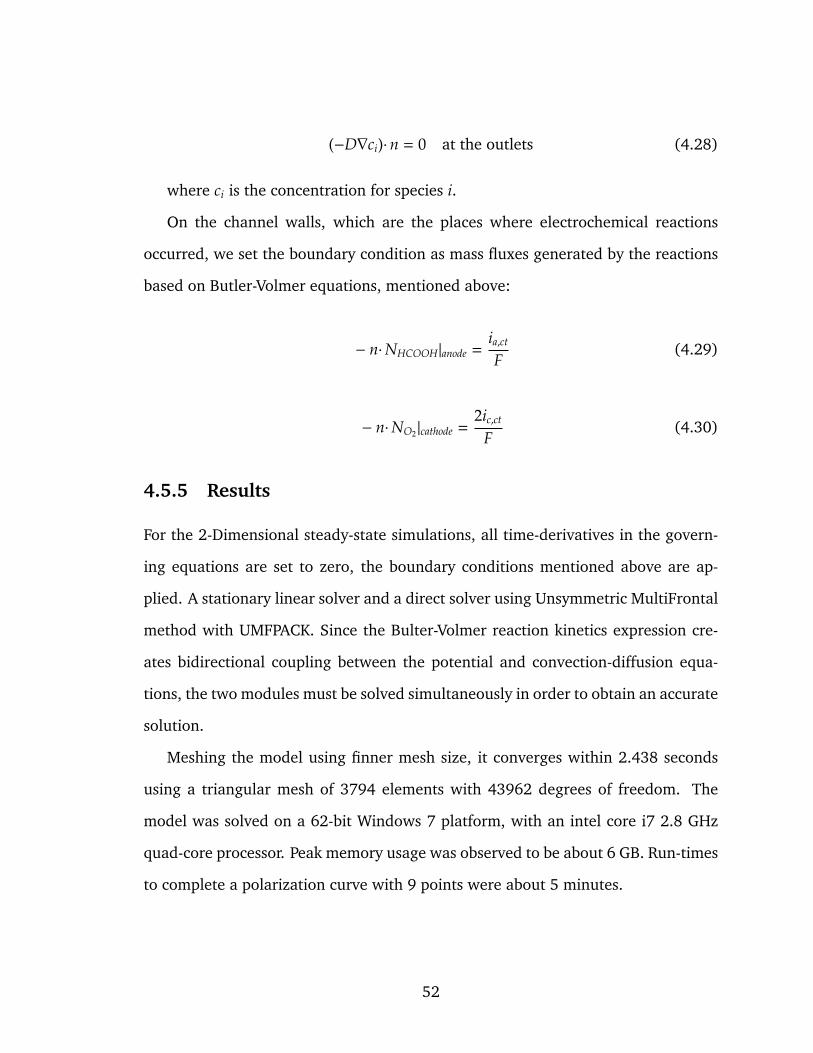
(−D∇ci)·n = 0 at the outlets (4.28)

where ci is the concentration for species i.

On the channel walls, which are the places where electrochemical reactions

occurred, we set the boundary condition as mass fluxes generated by the reactions

based on Butler-Volmer equations, mentioned above:

− n·NHCOOH|anode =ia,ct

F(4.29)

− n·NO2 |cathode =2ic,ct

F(4.30)

4.5.5 Results

For the 2-Dimensional steady-state simulations, all time-derivatives in the govern-

ing equations are set to zero, the boundary conditions mentioned above are ap-

plied. A stationary linear solver and a direct solver using Unsymmetric MultiFrontal

method with UMFPACK. Since the Bulter-Volmer reaction kinetics expression cre-

ates bidirectional coupling between the potential and convection-diffusion equa-

tions, the two modules must be solved simultaneously in order to obtain an accurate

solution.

Meshing the model using finner mesh size, it converges within 2.438 seconds

using a triangular mesh of 3794 elements with 43962 degrees of freedom. The

model was solved on a 62-bit Windows 7 platform, with an intel core i7 2.8 GHz

quad-core processor. Peak memory usage was observed to be about 6 GB. Run-times

to complete a polarization curve with 9 points were about 5 minutes.

52

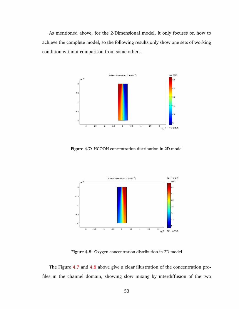
As mentioned above, for the 2-Dimensional model, it only focuses on how to

achieve the complete model, so the following results only show one sets of working

condition without comparison from some others.

Figure 4.7: HCOOH concentration distribution in 2D model

Figure 4.8: Oxygen concentration distribution in 2D model

The Figure 4.7 and 4.8 above give a clear illustration of the concentration pro-

files in the channel domain, showing slow mixing by interdiffusion of the two

53

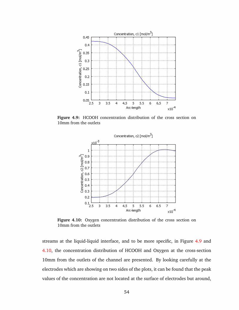
Figure 4.9: HCOOH concentration distribution of the cross section on10mm from the outlets

Figure 4.10: Oxygen concentration distribution of the cross section on10mm from the outlets

streams at the liquid-liquid interface, and to be more specific, in Figure 4.9 and

4.10, the concentration distribution of HCOOH and Oxygen at the cross-section

10mm from the outlets of the channel are presented. By looking carefully at the

electrodes which are showing on two sides of the plots, it can be found that the peak

values of the concentration are not located at the surface of electrodes but around,

54

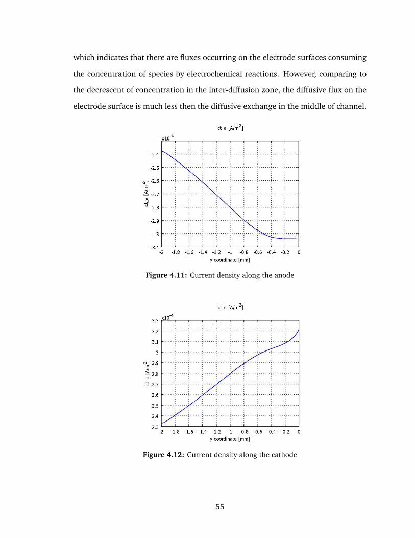
which indicates that there are fluxes occurring on the electrode surfaces consuming

the concentration of species by electrochemical reactions. However, comparing to

the decrescent of concentration in the inter-diffusion zone, the diffusive flux on the

electrode surface is much less then the diffusive exchange in the middle of channel.

Figure 4.11: Current density along the anode

Figure 4.12: Current density along the cathode

55

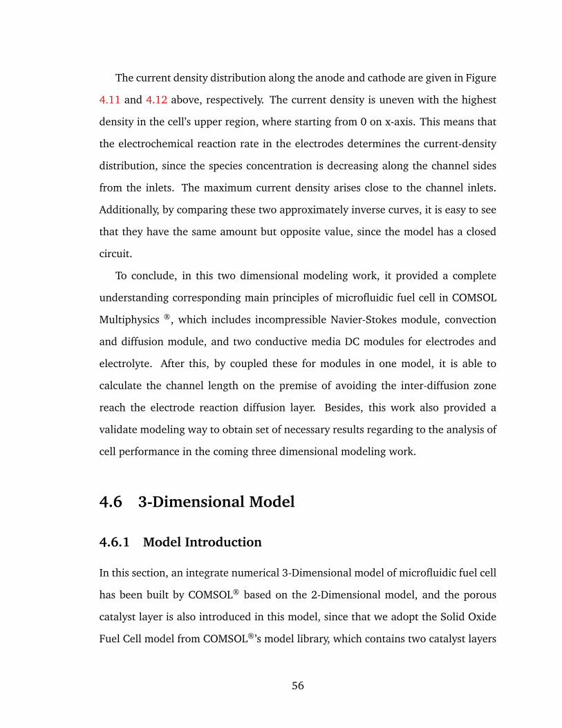
The current density distribution along the anode and cathode are given in Figure

4.11 and 4.12 above, respectively. The current density is uneven with the highest

density in the cell’s upper region, where starting from 0 on x-axis. This means that

the electrochemical reaction rate in the electrodes determines the current-density

distribution, since the species concentration is decreasing along the channel sides

from the inlets. The maximum current density arises close to the channel inlets.

Additionally, by comparing these two approximately inverse curves, it is easy to see

that they have the same amount but opposite value, since the model has a closed

circuit.

To conclude, in this two dimensional modeling work, it provided a complete

understanding corresponding main principles of microfluidic fuel cell in COMSOL

Multiphysics ®, which includes incompressible Navier-Stokes module, convection

and diffusion module, and two conductive media DC modules for electrodes and

electrolyte. After this, by coupled these for modules in one model, it is able to

calculate the channel length on the premise of avoiding the inter-diffusion zone

reach the electrode reaction diffusion layer. Besides, this work also provided a

validate modeling way to obtain set of necessary results regarding to the analysis of

cell performance in the coming three dimensional modeling work.

4.6 3-Dimensional Model

4.6.1 Model Introduction

In this section, an integrate numerical 3-Dimensional model of microfluidic fuel cell

has been built by COMSOL® based on the 2-Dimensional model, and the porous

catalyst layer is also introduced in this model, since that we adopt the Solid Oxide

Fuel Cell model from COMSOL®’s model library, which contains two catalyst layers

56

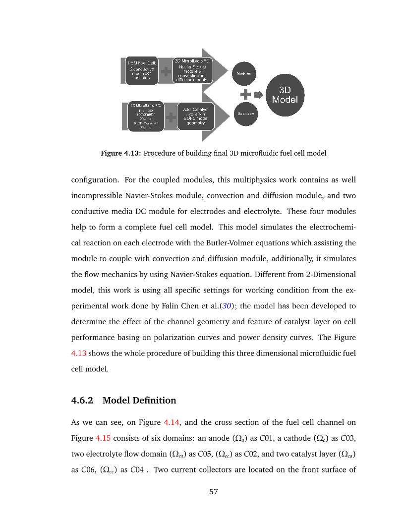
Figure 4.13: Procedure of building final 3D microfluidic fuel cell model

configuration. For the coupled modules, this multiphysics work contains as well

incompressible Navier-Stokes module, convection and diffusion module, and two

conductive media DC module for electrodes and electrolyte. These four modules

help to form a complete fuel cell model. This model simulates the electrochemi-

cal reaction on each electrode with the Butler-Volmer equations which assisting the

module to couple with convection and diffusion module, additionally, it simulates

the flow mechanics by using Navier-Stokes equation. Different from 2-Dimensional

model, this work is using all specific settings for working condition from the ex-

perimental work done by Falin Chen et al.(30); the model has been developed to

determine the effect of the channel geometry and feature of catalyst layer on cell

performance basing on polarization curves and power density curves. The Figure

4.13 shows the whole procedure of building this three dimensional microfluidic fuel

cell model.

4.6.2 Model Definition

As we can see, on Figure 4.14, and the cross section of the fuel cell channel on

Figure 4.15 consists of six domains: an anode (Ωa) as C01, a cathode (Ωc) as C03,

two electrolyte flow domain (Ωea) as C05, (Ωec) as C02, and two catalyst layer (Ωca)

as C06, (Ωcc) as C04 . Two current collectors are located on the front surface of

57

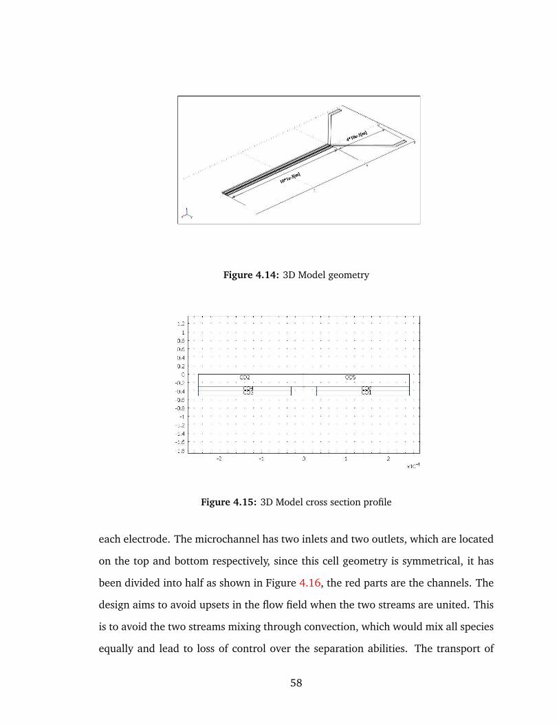
Figure 4.14: 3D Model geometry

Figure 4.15: 3D Model cross section profile

each electrode. The microchannel has two inlets and two outlets, which are located

on the top and bottom respectively, since this cell geometry is symmetrical, it has

been divided into half as shown in Figure 4.16, the red parts are the channels. The

design aims to avoid upsets in the flow field when the two streams are united. This

is to avoid the two streams mixing through convection, which would mix all species

equally and lead to loss of control over the separation abilities. The transport of

58

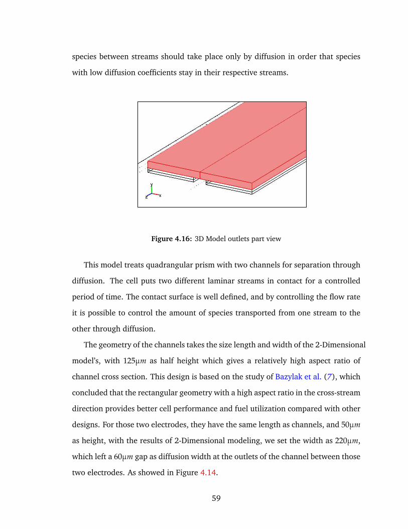
species between streams should take place only by diffusion in order that species

with low diffusion coefficients stay in their respective streams.

Figure 4.16: 3D Model outlets part view

This model treats quadrangular prism with two channels for separation through

diffusion. The cell puts two different laminar streams in contact for a controlled

period of time. The contact surface is well defined, and by controlling the flow rate

it is possible to control the amount of species transported from one stream to the

other through diffusion.

The geometry of the channels takes the size length and width of the 2-Dimensional

model’s, with 125µm as half height which gives a relatively high aspect ratio of

channel cross section. This design is based on the study of Bazylak et al. (7), which

concluded that the rectangular geometry with a high aspect ratio in the cross-stream

direction provides better cell performance and fuel utilization compared with other

designs. For those two electrodes, they have the same length as channels, and 50µm

as height, with the results of 2-Dimensional modeling, we set the width as 220µm,

which left a 60µm gap as diffusion width at the outlets of the channel between those

two electrodes. As showed in Figure 4.14.

59

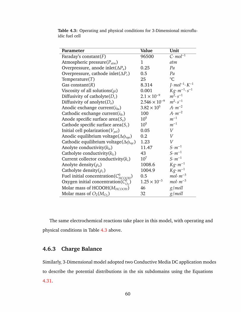
Table 4.3: Operating and physical conditions for 3-Dimensional microflu-idic fuel cell

Parameter Value UnitFaraday’s constant(F) 96500 C·mol−1

Atmospheric pressure(Patm) 1 atmOverpressure, anode inlet(∆Pa) 0.25 PaOverpressure, cathode inlet(∆Pc) 0.5 PaTemperature(T) 25 °CGas constant(R) 8.314 J·mol−1·K−1

Viscosity of all solutions(µ) 0.001 Kg·m−1· s−1

Diffusivity of catholyte(Dc) 2.1 × 10−9 m2· s−1

Diffusivity of anolyte(Da) 2.546 × 10−9 m2· s−1

Anodic exchange current(i0a) 3.82 × 105 A·m−2

Cathodic exchange current(i0c) 100 A·m−2

Anode specific surface area(Sa) 105 m−1

Cathode specific surface area(Sc) 105 m−1

Initial cell polarization(Vpol) 0.05 VAnodic equilibrium voltage(∆φeqa) 0.2 VCathodic equilibrium voltage(∆φeqc) 1.23 VAnolyte conductivity(kla) 11.47 S·m−1

Catholyte conductivity(klc) 43 S·m−1

Current collector conductivity(ks) 107 S·m−1

Anolyte density(ρa) 1008.6 Kg·m−1

Catholyte density(ρc) 1004.9 Kg·m−1

Fuel initial concentration(C0HCOOH) 0.5 mol·m−3

Oxygen initial concentration(C0O2

) 1.25 × 10−3 mol·m−3

Molar mass of HCOOH(MHCOOH) 46 g/mollMolar mass of O2(MO2) 32 g/moll

The same electrochemical reactions take place in this model, with operating and

physical conditions in Table 4.3 above.

4.6.3 Charge Balance

Similarly, 3-Dimensional model adopted two Conductive Media DC application modes

to describe the potential distributions in the six subdomains using the Equations

4.31.

60

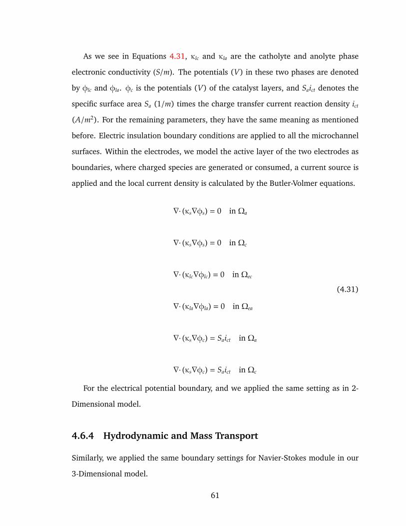
As we see in Equations 4.31, κlc and κla are the catholyte and anolyte phase

electronic conductivity (S/m). The potentials (V) in these two phases are denoted

by φlc and φla. φc is the potentials (V) of the catalyst layers, and Saict denotes the

specific surface area Sa (1/m) times the charge transfer current reaction density ict

(A/m2). For the remaining parameters, they have the same meaning as mentioned

before. Electric insulation boundary conditions are applied to all the microchannel

surfaces. Within the electrodes, we model the active layer of the two electrodes as

boundaries, where charged species are generated or consumed, a current source is

applied and the local current density is calculated by the Butler-Volmer equations.

∇· (κs∇φs) = 0 in Ωa

∇· (κs∇φs) = 0 in Ωc

∇· (κlc∇φlc) = 0 in Ωec

∇· (κla∇φla) = 0 in Ωea

∇· (κs∇φc) = Saict in Ωa

∇· (κs∇φc) = Saict in Ωc

(4.31)

For the electrical potential boundary, and we applied the same setting as in 2-

Dimensional model.

4.6.4 Hydrodynamic and Mass Transport

Similarly, we applied the same boundary settings for Navier-Stokes module in our

3-Dimensional model.

61

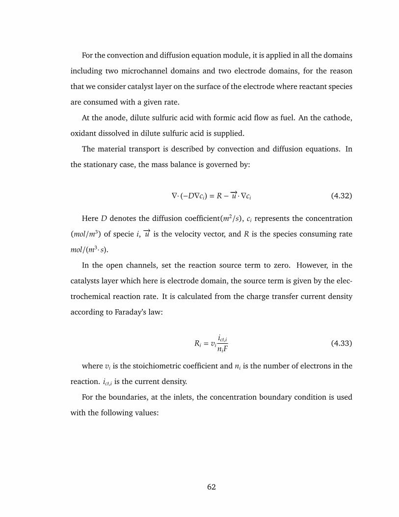
For the convection and diffusion equation module, it is applied in all the domains

including two microchannel domains and two electrode domains, for the reason

that we consider catalyst layer on the surface of the electrode where reactant species

are consumed with a given rate.

At the anode, dilute sulfuric acid with formic acid flow as fuel. An the cathode,

oxidant dissolved in dilute sulfuric acid is supplied.

The material transport is described by convection and diffusion equations. In

the stationary case, the mass balance is governed by:

∇· (−D∇ci) = R − −→u · ∇ci (4.32)

Here D denotes the diffusion coefficient(m2/s), ci represents the concentration

(mol/m3) of specie i, −→u is the velocity vector, and R is the species consuming rate

mol/(m3· s).

In the open channels, set the reaction source term to zero. However, in the

catalysts layer which here is electrode domain, the source term is given by the elec-

trochemical reaction rate. It is calculated from the charge transfer current density

according to Faraday’s law:

Ri = viict,i

niF(4.33)

where vi is the stoichiometric coefficient and ni is the number of electrons in the

reaction. ict,i is the current density.

For the boundaries, at the inlets, the concentration boundary condition is used

with the following values:

62

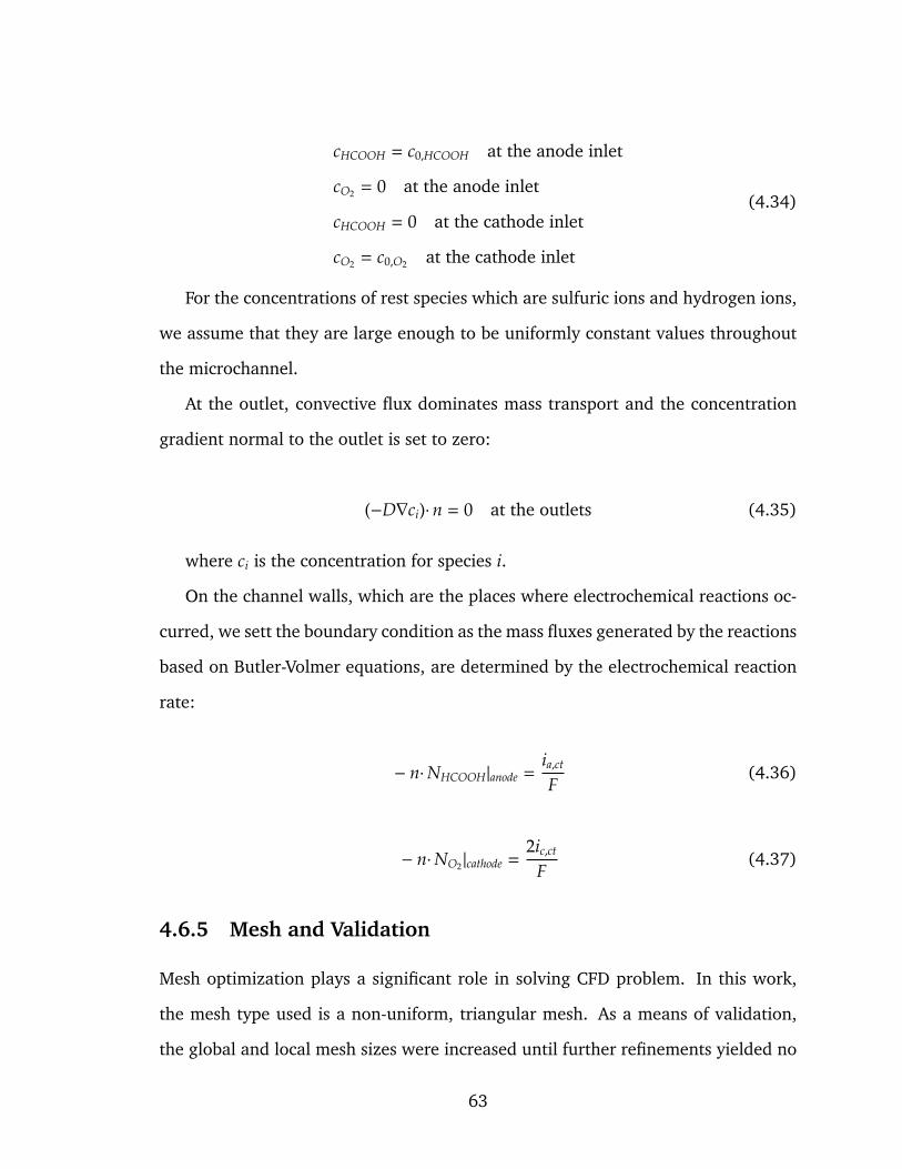
cHCOOH = c0,HCOOH at the anode inlet

cO2 = 0 at the anode inlet

cHCOOH = 0 at the cathode inlet

cO2 = c0,O2 at the cathode inlet

(4.34)

For the concentrations of rest species which are sulfuric ions and hydrogen ions,

we assume that they are large enough to be uniformly constant values throughout

the microchannel.

At the outlet, convective flux dominates mass transport and the concentration

gradient normal to the outlet is set to zero:

(−D∇ci)·n = 0 at the outlets (4.35)

where ci is the concentration for species i.

On the channel walls, which are the places where electrochemical reactions oc-

curred, we sett the boundary condition as the mass fluxes generated by the reactions

based on Butler-Volmer equations, are determined by the electrochemical reaction

rate:

− n·NHCOOH|anode =ia,ct

F(4.36)

− n·NO2 |cathode =2ic,ct

F(4.37)

4.6.5 Mesh and Validation

Mesh optimization plays a significant role in solving CFD problem. In this work,

the mesh type used is a non-uniform, triangular mesh. As a means of validation,

the global and local mesh sizes were increased until further refinements yielded no

63

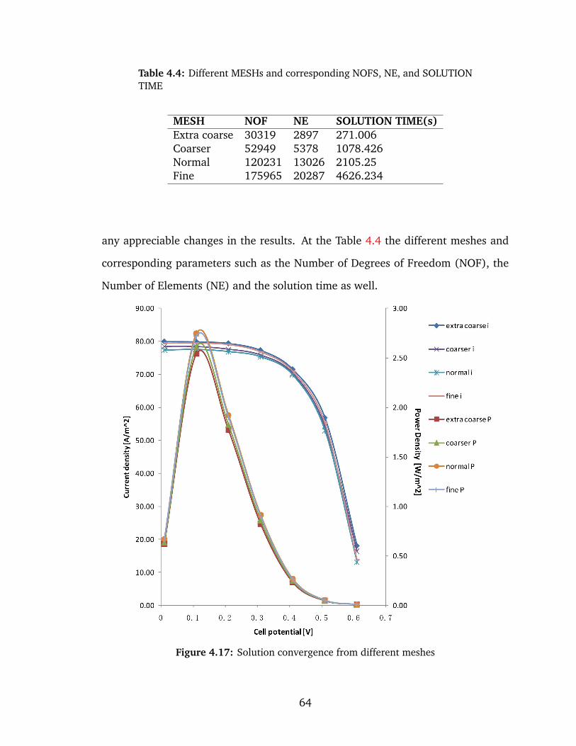
Table 4.4: Different MESHs and corresponding NOFS, NE, and SOLUTIONTIME

MESH NOF NE SOLUTION TIME(s)Extra coarse 30319 2897 271.006Coarser 52949 5378 1078.426Normal 120231 13026 2105.25Fine 175965 20287 4626.234

any appreciable changes in the results. At the Table 4.4 the different meshes and

corresponding parameters such as the Number of Degrees of Freedom (NOF), the

Number of Elements (NE) and the solution time as well.

Figure 4.17: Solution convergence from different meshes

64

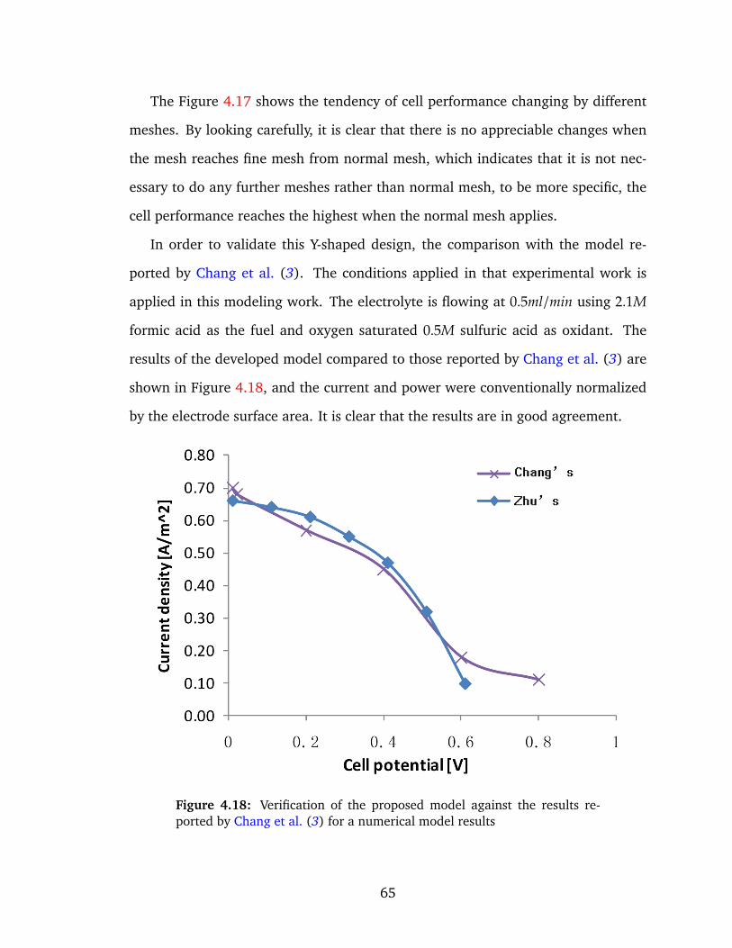
The Figure 4.17 shows the tendency of cell performance changing by different

meshes. By looking carefully, it is clear that there is no appreciable changes when

the mesh reaches fine mesh from normal mesh, which indicates that it is not nec-

essary to do any further meshes rather than normal mesh, to be more specific, the

cell performance reaches the highest when the normal mesh applies.

In order to validate this Y-shaped design, the comparison with the model re-

ported by Chang et al. (3). The conditions applied in that experimental work is

applied in this modeling work. The electrolyte is flowing at 0.5ml/min using 2.1M

formic acid as the fuel and oxygen saturated 0.5M sulfuric acid as oxidant. The

results of the developed model compared to those reported by Chang et al. (3) are

shown in Figure 4.18, and the current and power were conventionally normalized

by the electrode surface area. It is clear that the results are in good agreement.

Figure 4.18: Verification of the proposed model against the results re-ported by Chang et al. (3) for a numerical model results

65

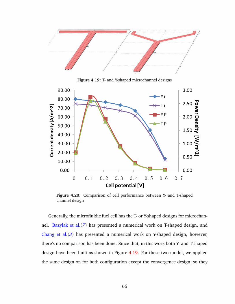
Figure 4.19: T- and Y-shaped microchannel designs

Figure 4.20: Comparison of cell performance between Y- and T-shapedchannel design

Generally, the microfluidic fuel cell has the T- or Y-shaped designs for microchan-

nel. Bazylak et al.(7) has presented a numerical work on T-shaped design, and

Chang et al.(3) has presented a numerical work on Y-shaped design, however,

there’s no comparison has been done. Since that, in this work both Y- and T-shaped

design have been built as shown in Figure 4.19. For these two model, we applied

the same design on for both configuration except the convergence design, so they

66

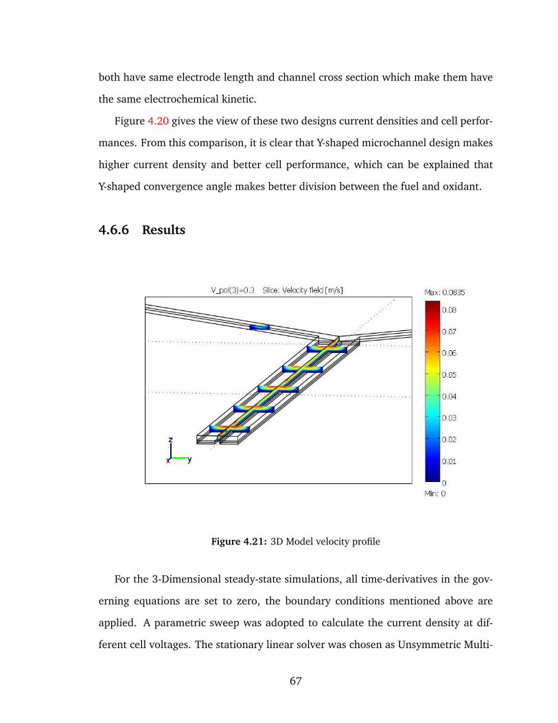
both have same electrode length and channel cross section which make them have

the same electrochemical kinetic.

Figure 4.20 gives the view of these two designs current densities and cell perfor-

mances. From this comparison, it is clear that Y-shaped microchannel design makes

higher current density and better cell performance, which can be explained that

Y-shaped convergence angle makes better division between the fuel and oxidant.

4.6.6 Results

Figure 4.21: 3D Model velocity profile

For the 3-Dimensional steady-state simulations, all time-derivatives in the gov-

erning equations are set to zero, the boundary conditions mentioned above are

applied. A parametric sweep was adopted to calculate the current density at dif-

ferent cell voltages. The stationary linear solver was chosen as Unsymmetric Multi-

67

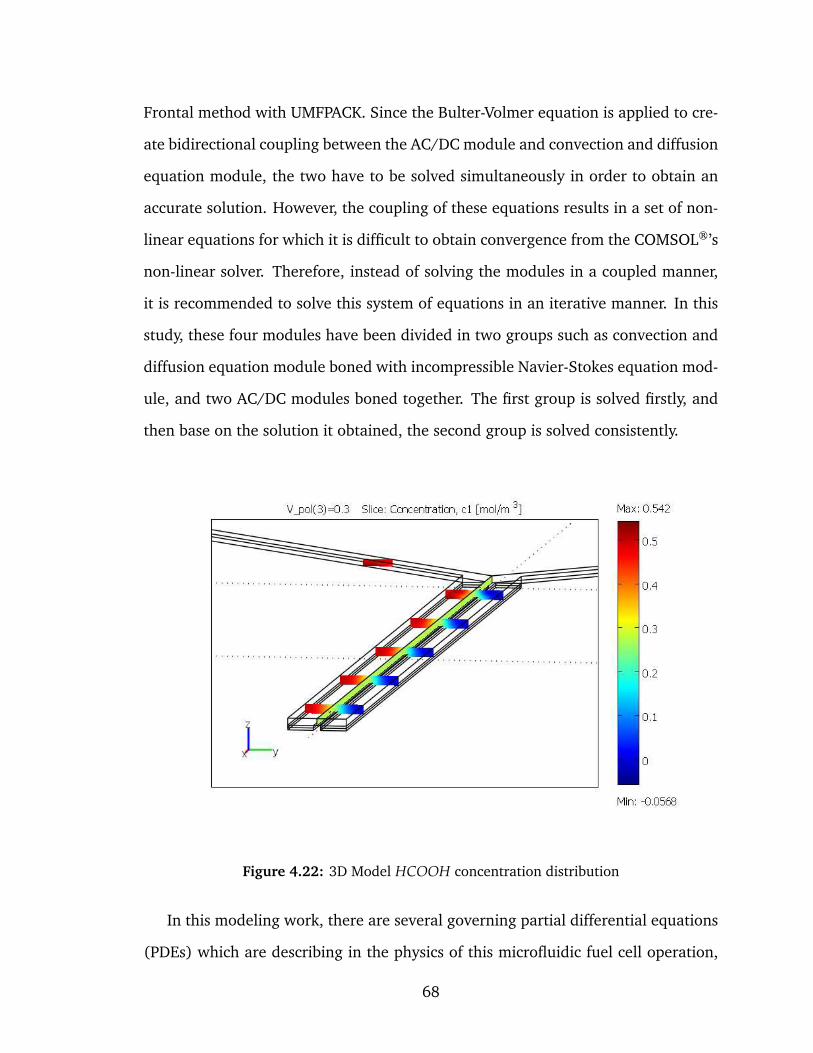
Frontal method with UMFPACK. Since the Bulter-Volmer equation is applied to cre-

ate bidirectional coupling between the AC/DC module and convection and diffusion

equation module, the two have to be solved simultaneously in order to obtain an

accurate solution. However, the coupling of these equations results in a set of non-

linear equations for which it is difficult to obtain convergence from the COMSOL®’s

non-linear solver. Therefore, instead of solving the modules in a coupled manner,

it is recommended to solve this system of equations in an iterative manner. In this

study, these four modules have been divided in two groups such as convection and

diffusion equation module boned with incompressible Navier-Stokes equation mod-

ule, and two AC/DC modules boned together. The first group is solved firstly, and

then base on the solution it obtained, the second group is solved consistently.

Figure 4.22: 3D Model HCOOH concentration distribution

In this modeling work, there are several governing partial differential equations

(PDEs) which are describing in the physics of this microfluidic fuel cell operation,

68

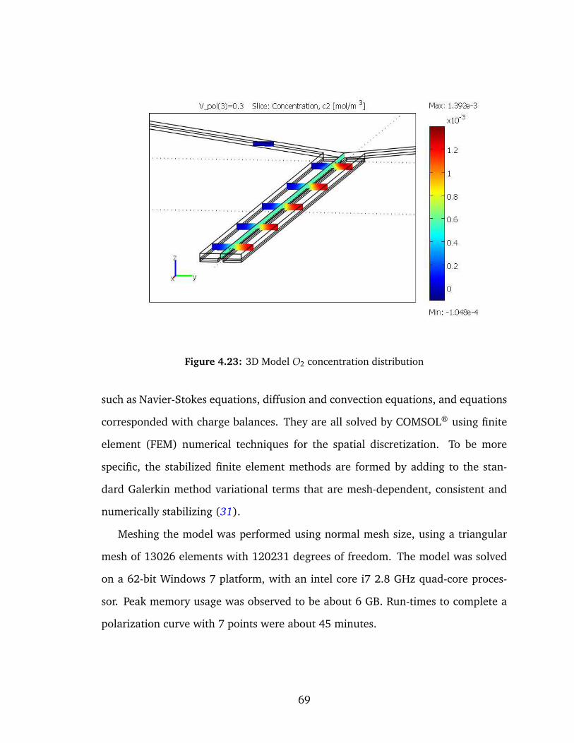
Figure 4.23: 3D Model O2 concentration distribution

such as Navier-Stokes equations, diffusion and convection equations, and equations

corresponded with charge balances. They are all solved by COMSOL® using finite

element (FEM) numerical techniques for the spatial discretization. To be more

specific, the stabilized finite element methods are formed by adding to the stan-

dard Galerkin method variational terms that are mesh-dependent, consistent and

numerically stabilizing (31).

Meshing the model was performed using normal mesh size, using a triangular

mesh of 13026 elements with 120231 degrees of freedom. The model was solved

on a 62-bit Windows 7 platform, with an intel core i7 2.8 GHz quad-core proces-

sor. Peak memory usage was observed to be about 6 GB. Run-times to complete a

polarization curve with 7 points were about 45 minutes.

69

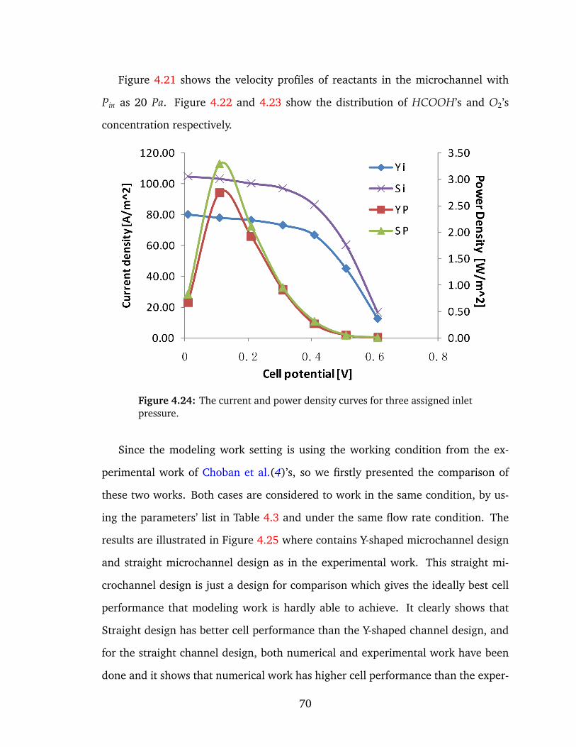
Figure 4.21 shows the velocity profiles of reactants in the microchannel with

Pin as 20 Pa. Figure 4.22 and 4.23 show the distribution of HCOOH’s and O2’s

concentration respectively.

Figure 4.24: The current and power density curves for three assigned inletpressure.

Since the modeling work setting is using the working condition from the ex-

perimental work of Choban et al.(4)’s, so we firstly presented the comparison of

these two works. Both cases are considered to work in the same condition, by us-

ing the parameters’ list in Table 4.3 and under the same flow rate condition. The

results are illustrated in Figure 4.25 where contains Y-shaped microchannel design

and straight microchannel design as in the experimental work. This straight mi-

crochannel design is just a design for comparison which gives the ideally best cell

performance that modeling work is hardly able to achieve. It clearly shows that

Straight design has better cell performance than the Y-shaped channel design, and

for the straight channel design, both numerical and experimental work have been

done and it shows that numerical work has higher cell performance than the exper-

70

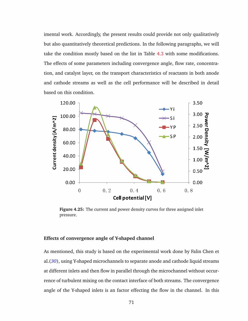
imental work. Accordingly, the present results could provide not only qualitatively

but also quantitatively theoretical predictions. In the following paragraphs, we will

take the condition mostly based on the list in Table 4.3 with some modifications.

The effects of some parameters including convergence angle, flow rate, concentra-

tion, and catalyst layer, on the transport characteristics of reactants in both anode

and cathode streams as well as the cell performance will be described in detail

based on this condition.

Figure 4.25: The current and power density curves for three assigned inletpressure.

Effects of convergence angle of Y-shaped channel

As mentioned, this study is based on the experimental work done by Falin Chen et

al.(30), using Y-shaped microchannels to separate anode and cathode liquid streams

at different inlets and then flow in parallel through the microchannel without occur-

rence of turbulent mixing on the contact interface of both streams. The convergence

angle of the Y-shaped inlets is an factor effecting the flow in the channel. In this

71

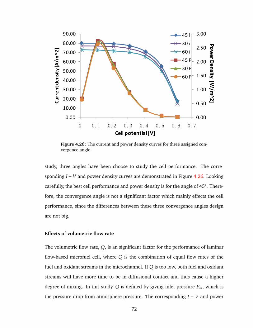
Figure 4.26: The current and power density curves for three assigned con-vergence angle.

study, three angles have been choose to study the cell performance. The corre-

sponding I−V and power density curves are demonstrated in Figure 4.26. Looking

carefully, the best cell performance and power density is for the angle of 45°. There-

fore, the convergence angle is not a significant factor which mainly effects the cell

performance, since the differences between these three convergence angles design

are not big.

Effects of volumetric flow rate

The volumetric flow rate, Q, is an significant factor for the performance of laminar

flow-based microfuel cell, where Q is the combination of equal flow rates of the

fuel and oxidant streams in the microchannel. If Q is too low, both fuel and oxidant

streams will have more time to be in diffusional contact and thus cause a higher

degree of mixing. In this study, Q is defined by giving inlet pressure Pin, which is

the pressure drop from atmosphere pressure. The corresponding I − V and power

72

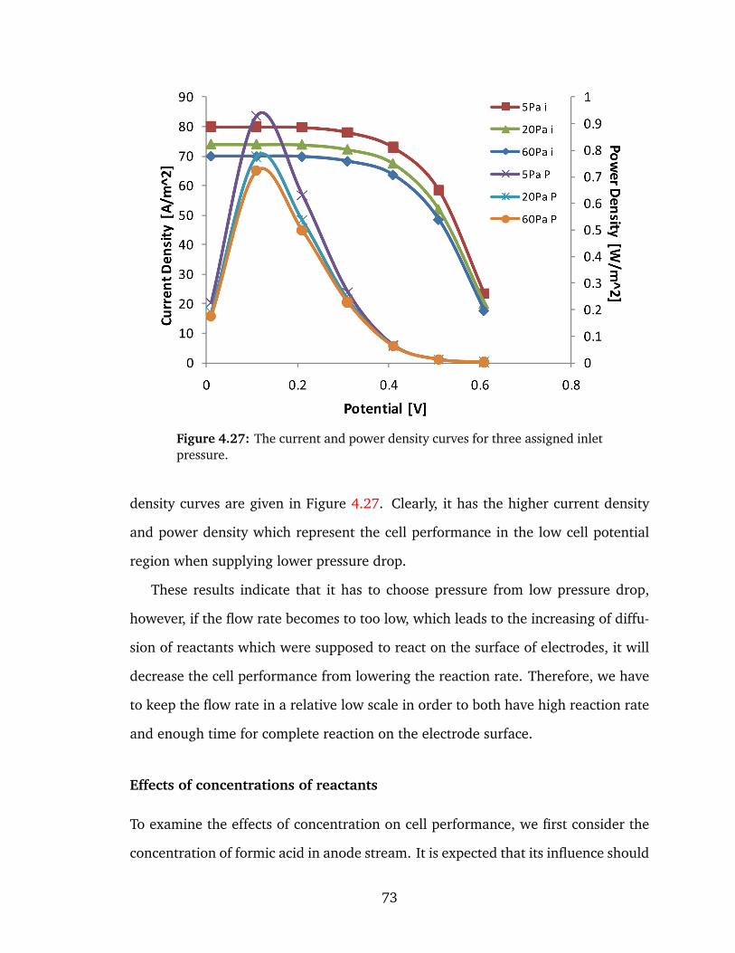
Figure 4.27: The current and power density curves for three assigned inletpressure.

density curves are given in Figure 4.27. Clearly, it has the higher current density

and power density which represent the cell performance in the low cell potential

region when supplying lower pressure drop.

These results indicate that it has to choose pressure from low pressure drop,

however, if the flow rate becomes to too low, which leads to the increasing of diffu-

sion of reactants which were supposed to react on the surface of electrodes, it will

decrease the cell performance from lowering the reaction rate. Therefore, we have

to keep the flow rate in a relative low scale in order to both have high reaction rate

and enough time for complete reaction on the electrode surface.

Effects of concentrations of reactants

To examine the effects of concentration on cell performance, we first consider the

concentration of formic acid in anode stream. It is expected that its influence should

73

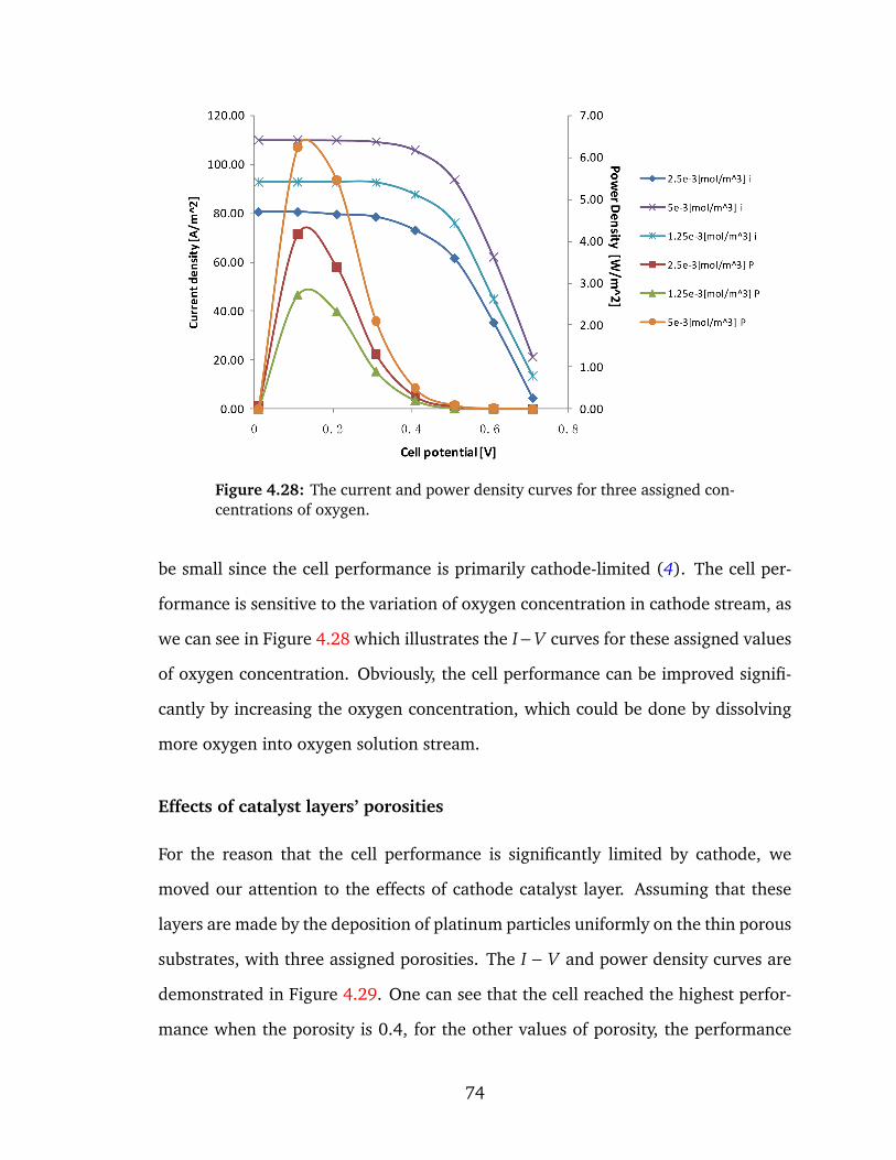
Figure 4.28: The current and power density curves for three assigned con-centrations of oxygen.

be small since the cell performance is primarily cathode-limited (4). The cell per-

formance is sensitive to the variation of oxygen concentration in cathode stream, as

we can see in Figure 4.28 which illustrates the I−V curves for these assigned values

of oxygen concentration. Obviously, the cell performance can be improved signifi-

cantly by increasing the oxygen concentration, which could be done by dissolving

more oxygen into oxygen solution stream.

Effects of catalyst layers’ porosities

For the reason that the cell performance is significantly limited by cathode, we

moved our attention to the effects of cathode catalyst layer. Assuming that these

layers are made by the deposition of platinum particles uniformly on the thin porous

substrates, with three assigned porosities. The I − V and power density curves are

demonstrated in Figure 4.29. One can see that the cell reached the highest perfor-

mance when the porosity is 0.4, for the other values of porosity, the performance

74

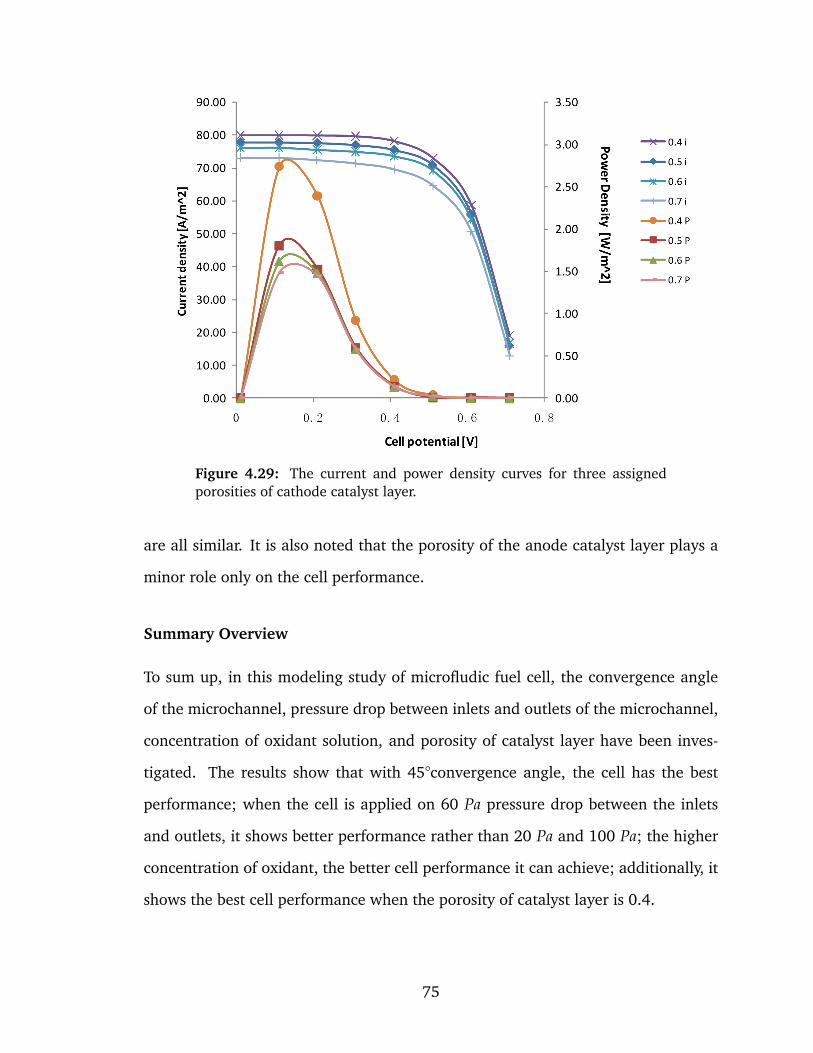
Figure 4.29: The current and power density curves for three assignedporosities of cathode catalyst layer.

are all similar. It is also noted that the porosity of the anode catalyst layer plays a

minor role only on the cell performance.

Summary Overview

To sum up, in this modeling study of microfludic fuel cell, the convergence angle

of the microchannel, pressure drop between inlets and outlets of the microchannel,

concentration of oxidant solution, and porosity of catalyst layer have been inves-

tigated. The results show that with 45°convergence angle, the cell has the best

performance; when the cell is applied on 60 Pa pressure drop between the inlets

and outlets, it shows better performance rather than 20 Pa and 100 Pa; the higher

concentration of oxidant, the better cell performance it can achieve; additionally, it

shows the best cell performance when the porosity of catalyst layer is 0.4.

75

Chapter 5CONCLUSIONS AND FUTURE DIRECTIONS

In this dissertation, the background and motivation for microfluidic fuel cells

were presented in chapter 1, as well as the particular objectives; A litera-

ture review of this field was provided in chapter 2, as well as numbers of

preliminary work based on the experiments for mocrofluidic fuel cell model-

ing were discussed; The theoretical and numerical studies on microfluidic fuel cells

were presented in chapter 3 and 4 respectively. In this chapter, conclusions and

contributions will be presented, as well as the future work.

5.1 Conclusion and Contribution

A theoretical study about microfluidic fuel cells has been presented on three general

aspects: such as mass transfer, hydrodynamics, and electrochemistry. Subsequently,

we conducted a numerical analysis to study the performance of a laminar flow-

based microfluidic fuel cell consisting of a Y-shaped microchannel. Three dimen-

sional models for the microfluidic fuel cell have been developed in this work. The

76

models were applied to investigate species transport, hydrodynamics and electro-

chemical reaction in six domains of electrodes, catalyst layers, and microchannels.

In this thesis the catalyst layers were modeled as two finite domains rather than

just two boundaries. A laminar flow field is used to investigate the species transfer.

Two conductive media DC modules representing electronic transport in the external

circle and ionic transport in the internal circle respectively were used to model the

electric fields within the fuel cell. The commercial software, COMSOL Multiphysics

®, was used to solve the governing equations numerically. A detailed analysis on

the species transport and electrochemical reaction was put forward for an isother-

mal, single phase case. Afterward, a discussion about the effects of the convergence

angle of the Y-shaped channel, the volumetric flow rate (pressure drop), the con-

centration of reactants, and the catalyst layers’ porosities on the cell performances

are given successively.

This numerical work uses the same conditions as the experimental work of

Choban et al.(4) where the authors used a planar channel design, but for the nu-

merical work it apply the straight channel and Y-shaped channel. The results show

a good concordance and that the straight channel design numerical model provides

67% higher power density than the planar channel design experimental work. One

the other hand, for the Y-shaped design, its performance is lower than the experi-

mental work. However, the planar channel design requires a significant difference

in density between the top flow and the bottom flow. This is not the case for the

Y-shaped design. Most importantly, the power density of the ideal straight design

is twice higher than Y-shaped design’s, it indicates that there is significant potential

space to improve the cell performance by modifying the channel geometry.

The first group of modeling on different convergence angles has confirmed that

Y-shaped microchannel with 45° convergence angle has the maximum cell perfor-

mance compared with 30°and 60° designs. The geometry of the cell plays a critical

77

role in the performance of the cell, which is limited by the mass transport of reac-

tants through the concentration boundary layers to the electrodes.

After the Y-shaped microchannel with 45°convergence angle designed has been

proved that provides a better cell performance, this design has been used to investi-

gate cell models with three sets of pressure drops in the channel. The results show

that the flow rate in the channel significantly effects the cell performance, because

comparing 100 Pa and 60 Pa pressure drop, the cell performance was tremendously

improved by 5 Pa. Therefore, lowering the inlet velocity from a high value results

in a significant improvement in fuel utilization by increasing the reaction time of

electrochemical reactions on the electrode surface with a minimal increase in cross

stream mixing at the outlet; However, on the other hand, when the velocity goes

too low, it will decrease the fuel utilization by consuming the reactant on the fuel

crossover resulted from low flow rate.

After setting the convergence angle and pressure drop,the effects of concentra-

tion on cell performance has been examined . Firstly, it only considered the con-

centration of formic acid in the anode stream. It was expected that its influence

should be small since the cell performance is primarily cathode-limited. Contrarily,

the variation of oxygen concentration can particularly effect the cell performance,

and elevating the concentration of oxygen in the solution can significantly improve

the cell performance.

For the catalyst layers, a modeling study has been made on the porosity of them.

Since the fuel cell is cathode-limited, the porosity of the anode catalyst layer plays

a minor role only on the cell performance. The modeling of the cathode catalyst

layer with different porosity showed that the 0.4 porosity case has the highest cell

performance over the 0.5, 0.6, and 0.7 cases. Therefore, by modifying the catalyst

layers can help improve the cell performance.

78

5.2 Future Directions

The present results provide an overview for the characteristics of this microfluidic

fuel cell model and also benefit the further design work to optimize the cell perfor-

mance. Some of opportunity for future work is outlined below.

From what it shows in Figure ??, it still has a big difference on cell performance

between this Y-shaped design modeling work and the theoretical ideal modeling

design. It indicates that by improving the channel design in a better way, it still can

significantly obtain a better cell performance.

Considering the oxygen concentration is an important factor effecting the cell

performance and it is difficult to dissolve the gaseous oxygen into solution to obtain

a high concentration, exploration of a new liquid oxidant is very interesting for

future improvements.

Additionally, the microchannels have to continue to be tested and their length,

width, and thickness optimized to give the maximum power density using a mini-

mum physical area. As well as the material choosing for the channel fabrication can

be done by Spark assisted chemical engraving (SACE) machining in Dr. Wuthrich’s

lab. SACE is a novel method for 3D microstructuring of glass or other nonconduc-

tive materials with high aspect ratio and smooth surface quality (5).

The catalyst layer has been always considered as one of the most significant

aspects of cell performance improvement. Choosing different catalyst materials,

and modifying the layer configuration could be investigated to enhance the electro-

chemical reaction, as well as the electrode design.

Finally, since the experimental work of Choban et al.(4) offers a better cell per-

formance than the Y-shaped modeling work by using planar channel design, it will

be very interesting to test our Y-shaped channel but with vertical planner design for

79

the specific case when there is a significant difference in density between the top

flow and the bottom flow.

80

REFERENCES

[1] Bruus, H. Theoretical Microfluidics 2007, 48 – 51.

[2] Leo J. M. J. Blomen, M. N. M. Fuel Cell Systems 1993, 81 – 84.

[3] Chang, M.-H.; Chen, F.; Fang, N.-S. Analysis of membraneless fuel cell using

laminar flow in a Y-shaped microchannel. Journal of Power Sources 2006, 159,

810 – 816.

[4] Choban, E. R.; Markoski, L. J.; Wieckowski, A.; Kenis, P. J. A. Microfluidic fuel

cell based on laminar flow. Journal of Power Sources 2004, 128, 54 – 60.

[5] Wuthrich, R.; Fascio, V. Machining of non-conducting materials using electro-

chemical discharge phenomenon–an overview. International Journal of Ma-

chine Tools and Manufacture 2005, 45, 1095 – 1108.

[6] Kjeanga, E.; Djilali, N.; Sintona, D. Microfluidic fuel cells: A review. Journal of

Power Sources 2009, 186, 353 – 2369.

[7] Bazylak, A.; Sinton, D.; Djilali, N. Improved fuel utilization in microfluidic fuel

cells: A computational study. Journal of Power Sources 2005, 143, 57 – 66.

[8] Choban, E.; Markoski, L.; Stoltzfus, J.; Moore, J.; Kenis, P. Microfluidic Fuel

Cells that Lack a PEM. Power Sources Proc. 2002, 40, 317 – 320.

81

[9] Martinelli, M.; Viktorov, V. Modelling of laminar flow in the inlet section of

rectangular microchannels. Journal of Micromechanics and Microengineering

2009, 19, 025013 (9pp).

[10] Lee,; Jinkee,; Palmore,; R., G. T.; Tripathi,; Anubhav, Optimization of Mi-

crofluidic Fuel Cells Using Transport Principles. Analytical Chemistry 2007,

79, 7301 – 7307.

[11] Compton, R. G.; Pilkington, M. B. G.; Stearn, G. M. Mass Transport in Channel

Electrodes. Chemical Society 1988, 84, 2155 – 2171.

[12] Ismagilov, R. F.; Stroock, A. D.; Kenis, P. J. A.; Whitesides, G.; Stone, H. A.

Experimental and theoretical scaling laws for transverse diffusive broadening

in two-phase laminar flows in microchannels. Applied Physics Letters 2000, 76,

2376–2378.

[13] Phirani, J.; Basu, S. Analyses of fuel utilization in microfluidic fuel cell. Jour-

nal of Power Sources 2008, 175, 261 – 265.

[14] Chen, W.; Chen, F. Theoretical approaches to studying the single and simul-

taneous reactions in laminar flow-based membraneless fuel cells. Journal of

Power Sources 2006, 162, 1137 – 1146, Special issue including selected pa-

pers from the International Power Sources Symposium 2005 together with

regular papers.

[15] Kjeang, E.; Michel, R.; Harrington, D. A.; Sinton, D.; Djilali, N. An alkaline

microfluidic fuel cell based on formate and hypochlorite bleach. Electrochimica

Acta 2008, 54, 698 – 705.

[16] Kjeang, E.; Michel, R.; Harrington, D. A.; Sinton, D.; Djilali, N. A Microflu-

idic Fuel Cell with Flow-Through Porous Electrodes. Journal of the American

Chemical Society 2008, 130, 4000 – 4006.

82

[17] Kjeang, E.; McKechnie, J.; Sinton, D.; Djilali, N. Planar and three-dimensional

microfluidic fuel cell architectures based on graphite rod electrodes. Journal

of Power Sources 2007, 168, 379 – 390.

[18] Kjeang, E.; Proctor, B. T.; Brolo, A. G.; Harrington, D. A.; Djilali, N.; Sinton, D.

High-performance microfluidic vanadium redox fuel cell. Electrochimica Acta

2007, 52, 4942 – 4946.

[19] Choban, E.; Spendelow, J.; Gancs, L.; Wieckowski, A.; Kenis, P. Membrane-

less laminar flow-based micro fuel cells operating in alkaline, acidic, and

acidic/alkaline media. Electrochimica Acta 2005, 50, 5390 – 5398.

[20] Chen, F.; Chang, M.-H.; Hsu, C.-W. Analysis of membraneless microfuel cell

using decomposition of hydrogen peroxide in a Y-shaped microchannel. Elec-

trochimica Acta 2007, 52, 7270 – 7277.

[21] Lu, Y.; Reddy, R. G. Investigation of micro-PEM fuel cell using experimental

and modeling methods. Electrochimica Acta 2009, 54, 3952 – 3959.

[22] Mann, R.; Amphlett, J.; Peppley, B.; Thurgood, C. Application of Butler-Volmer

equations in the modelling of activation polarization for PEM fuel cells. Jour-

nal of Power Sources 2006, 161, 775 – 781.

[23] Cheddie, D. F.; Munroe, N. D. Three dimensional modeling of high tempera-

ture PEM fuel cells. Journal of Power Sources 2006, 160, 215 – 223.

[24] Al-Baghdadi, M. A. S.; Al-Janabi, H. A. S. Modeling optimizes PEM fuel

cell performance using three-dimensional multi-phase computational fluid dy-

namics model. Energy Conversion and Management 2007, 48, 3102 – 3119.

83

[25] Yoon, S. K.; Fichtl, G. W.; Kenis, P. J. A. Active control of the depletion bound-

ary layers in microfluidic electrochemical reactors. Lab on a Chip 2006, 6,

1516–1524.

[26] Spiegel, C. Modeling Micro Fuel Cells 2008, 299 – 334.

[27] Zhao, T. Micro Fuel Cells 2009, 105 – 106.

[28] Britz, D. Digital Simulation in Electrochemistry 2005, 5.

[29] Cottrell, F. G. Residual current in galvanic polarization. The Journal of Physical

Chemistry 1903, 42, 385 – 431.

[30] Chen, F.; Chang, M.-H.; Lin, M.-K. Analysis of membraneless formic acid mi-

crofuel cell using a planar microchannel. Electrochimica Acta 2007, 52, 2506

– 2514.

[31] Yazdani, A.; Shojai, L. Solution of a Scalar Convection-Diffusion Equation Us-

ing FEMLAB. COMSOL Multiphysics User’s Conference 2005 Boston 2005.

84