Sommerfeld Theory

1

2.1 Fermi Statistics and Fermi Surface Since Drude model, it took a quarter of a century for a breakthrough to occur. That arose from the development of quantum mechanics and recognition that electrons are fermions. In the Sommerfeld Free Electron Model, electrons are treated as being free and independent as in the Drude’s model. However, the classical Maxwell-Boltzmann (MB) distribution is replaced by the Fermi-Dirac (FD) distribution:

1]/)exp[(

1)(

TkEEf

B, (2.1)

where f(E) is the probability that a state with energy E is occupied by an electron at temperature T, kB is the Boltzmann’s constant and is the chemical potential of the system. Recall that the chemical potential is defined by the following normalization condition:

The no. of e- per unit volume, )()( EgEdEfn , (2.2)

where g(E) is the density of electron levels at energy E per unit volume of the specimen. It is convenient to think of the temperature, T0, defined by T0 = /kB. For metals, it is typically ~104 K. Because T0 is much bigger than room temperature (~300 K), the FD distribution does not vary much from T = 0 K to typical experimental temperatures. It is therefore of practical interest to examine the consequences of replacing the MB distribution by the FD distribution at T = 0 K. (i) Sommerfeld Model at T = 0 At T = 0, the electron gas is at its ground state. Since the electrons are assumed to be independent, we may solve the wave function i(r) and energy i for a single electron bounded inside the volume of the metal and then extend the solution to the N-electron case by simply writing the energy of the system to be i

N i. Because the electrons are assumed to be free, the single-electron wave function satisfies the Schrödinger’s equation of a free particle:

)()(2

22

rrm

. (2.3)

For mathematical convenience, we choose the boundary condition as such that the metal is a cube of side L = V1/3, where V is the volume of the specimen and assumed to be much bigger than the inter-ionic separation. We argue that this assumption about the boundary condition does not comprise the generality of the solution. It is because when the size of a system is sufficiently large, its (bulk) properties should not depend on its specific outer dimensions as observed in real life. To solve eqn (2.3), we also need to specify the boundary values of the wave function. To this end, we adopt the periodic boundary condition:

Fermi Statistics and Fermi Surface

Sommerfeld Theory

2

x, y, z + L) = x, y, z),

x, y + L, z) = x, y, z)

x + L, y, z) = x, y, z), (2.4) where nx, ny, and nz are integers. This choice, as opposed to ones that leads to standing wave solutions (obtained by setting specific values for the wave function at the boundaries), is motivated by our ultimate goal to find the properties of the electrons while itinerant. It is straightforward to show that the solution to eqn. 2.3 subject to the boundary condition (2.4) is:

,1

)( rki

ke

Vr

(2.5)

with energy

m

kk

2)(

22 , (2.6)

where k = |k|. In eqn. 2.5, use has been made of the normalization condition,

.1)(23 rrd

k

Notice that in eqn. 2.5, we have labeled the wavefunction by the

wavevector k. By eqn. (2.6), it is evident that k defines the eigen state energy. At the same time, k also defines a momentum eigen state as follows (You may notice that this simultaneity arises from the fact that the free-particle Hamiltonian commutes with the momentum operator.):

).()()( rkrirpkkk

(2.7)

This reveals that ħk is the momentum observable of the electron. As in the Drude model, it is convenient to use the velocity of the electrons in figuring the transport properties. Given that k(r) is a simultaneous eight function of the Hamiltonian and momentum operator, the velocity of the electron is:

v = p/m = mk /

. (2.9)

Using this, (k) can be rewritten in the familiar classical form:

222

2

1

2)( mv

m

kk

. (2.10)

Notice also from eqn. (2.5) that the wave function is an iterant plane wave with wavevector k, or wavelength, k.

Sommerfeld Theory

3

In the Drude model, we had assumed average values as <> = 3kBT/2, <vx> = <vy> = <vz> = (kBT/m)1/2 and cv = 3nkB for the electrons at equilibrium at temperature T. These values spring from the MB distribution assumed for the electrons. To adapt the discussions in the framework of the Sommerfeld model, we need to replace all these values by those appropriate to the FD distribution of eqn. (2.1), subject to the constraint of eqn. (2.2). In the following, we shall discuss how <>, the velocity relevant to the transport properties, and cv can be derived.

Typically, one starts by thinking how the electrons fill themselves into the allowed energy levels, (k). At T = 0 K, the answer is straightforward -- because electrons are fermions, they first fill the lowest energy level until all the degenerate states are filled, they begin to fill the next higher energy level. This picture brings about the necessity to be able to count the number of degeneracy of an energy level. This is related to the density of levels, g() mentioned above, which we shall derive later. We first derive the related quantity, g(k) - the density of states, which is the number of states contained in a unit volume in the so-called k-space that we shall next discuss.

By the periodic boundary condition, we have:

L

nk

L

nk

L

nk z

zy

yx

x

2,

2,

2 , nx, ny, nz integers. (2.12)

The space, made up of the axes kx, ky and kz is called the k-space. Apparently, the allowed states of the electrons constitute the set of points defined by eqn. 2.12 in the k-space. Clearly, each of such points occupies the SAME volume (2/L)d in the k-space, where d is the dimensionality of the system. For a 3 dimensional system, the density of states is:

g(k) = (L/2)3 = V/83 . (2.13) But eqn. 2.13 does not fully describe the density of states. It is because each k-state can accommodate two electrons because of the electron spins (allowed to be either up or down). Therefore, the accurate expression is:

g(k) = V/43 . (2.13) Notice that g(k) increases with V, the volume of the specimen. Physically, it means that the number of available states increases in proportion to the size of the system, which is intuitive. To remove the non-intrinsic factor, V, one commonly normalize the density of states by V. Unfortunately, the resultant quantity is also commonly called the density of states. Please beware of this when you come across discussions concerning the density of states. As stated above, at T = 0 K the electrons fill the lowest-energy unoccupied states first before filling those in the next higher energy level. Since (k) ~ k2, the states with a smaller radius k in the k-space get occupied first. So at T = 0 K, all the states enclosed by the sphere with radius, kF, in the k-space will be filled, where

Sommerfeld Theory

4

VkVk

N FF2

3

3

3

32

83

4

. (2.14)

Here, N is the total number of valence electrons in the metal. This sphere, known as the Fermi sphere, separates the occupied from the unoccupied states. Writing n = N/V, the electron density, we have:

3/12 )3( nkF (2.15) To get an idea about the size of kF, we make use of the parameter, rs,= [3/(4n)]1/3 introduced in eqn. 1.2. This gives

kF = 1.9/rs. (2.16) Recall that rs varies from 1.87a0 to 5.62a0, where a0 =

22 / me = 0.529 Å is the Bohr radius. It follows that kF is of the order of Å-1. The corresponding deBroglie wavelength, F = 2/ kF is thus of the order of Å or atomic spacing. The Fermi velocity, corresponding to the velocity of the most energetic electrons, is:

16102.2

ms

rk

mv

sFF

. (for rs in Å) (2.17)

Eqn. 2.17 illustrates that the Fermi velocity is very large, about 1% the speed of light even at T = 0 K. In contrast, the electron velocity in the Drude model is assumed to be thermal and is only ~105 ms-1 at room temperature, and decreases like ~T1/2 as T is decreased. Later we shall see that at experimental temperature (i.e., T a few hundred K) only those electrons near the Fermi surface actively participate in the transport phenomena and so vF is the relevant velocity to use in describing them. Moreover, vF, like , does not vary much with temperature. These lead to notable revisions to the values of some quantities previously considered by Drude. It is convenient to write the Fermi energy as:

20

0

222

22ak

a

e

m

kF

FF

(2.18)

Here, e2/2a0, known as the rydberg (Ry), is the ground-state binding energy of the hydrogen atom = 13.6 eV. Using eqn. 2.16, we can re-write Eqn. 2.18 as:

.)/(

502

0ar

eV

sF (2.19)

This shows that F is typically several eV, i.e., ~100 times the thermal energy at room temperature, which is ~0.025 eV. Correspondingly, the Fermi temperature, defined to be TF = F/kB is ~104 K. As pointed out above, because the Fermi temperature is much bigger

Sommerfeld Theory

5

than room temperature, the FD does not vary much with T for typical temperatures of interest. The ground state energy, U, for the N-electrons system is just the sum of the energies of all the k-states up to |k| = kF, multiplied by 2:

.||2

2||

22

Fkk

km

U

(2.20)

Because dk3 ~ (2/L)3 << kF, the set of points representing the allowed electron states effectively forms a continuum inside the space contained by the Fermi sphere. In that case, we may approximate the summation in eqn. (2.20) or other summations over k by replacing the summation operator (1/V)k by the following integral operator:

38

1lim

kd

V kV

, (2.22)

With this, eqn. 2.20 can be re-written as:

F

F

kF

kk m

kk

mdkkk

mkd

V

U

0

52

22

22

32

2

3 10

1

24

4

1

24

1

. (2.23)

Multiplying U/V by V/N, we obtain the average energy per electron. By further using eqn. 2.14 for N/V, we obtain:

U/N = 3F/5. (2.24) This result says that the average energy of the electrons is ~eV even at T = 0 K. This should be contrasted with the assumption of the Drude that the average energy of the electrons vanishes as T approaches 0 K. The Free Electron Gas at Finite Temperatures In the above, we have calculated that the chemical potential, F = ħ2kF

2/2m ( 3/12 )3( nkF ) at T = 0 K. At finite T, deviates from F(T = 0), and we need to use the

FD distribution at finite T to find the value of , defined by:

,1

1/)(

TkiBie

f (2.25)

and

iifN , (2.26)

Sommerfeld Theory

6

where i denotes the label for the allowed energy levels, which is obviously related to k. 2.2 The Electronic Heat Capacity – The linear T-dependence To evaluate the electronic specific heat capacity, cv, we must first calculate the total energy (U) per unit volume (V), u (= U/V):

)).((4

)(3

kfk

kdukall

(2.28)

The normalization condition (eqn. 2.26) in integral form or eqn. 2.2 is:

)).((4

13

kfkdnkall

(2.29)

In evaluating integrals like eqns. 2.28 and 2.29 of the form

)),((4

13

kFkdkall

(2.30)

one often makes use of the relation m

kk

2)(

22 . Given this, F((k)) has spherical

symmetry in the k-space and so we may write:

dk = 4k2dk (0< k < ) (2.31)

Now, dkm

kkd

2

)(

and 2

)(2

km

k

. Eqn. 2.31 can be written as:

.)(2

422

mdkmkd (2.32)

Hence Eqn. 2.30 becomes:

0

),()( Fgd where (2.33)

.)(2

)(222

kmmg

(2.34)

Sommerfeld Theory

7

As mentioned above, g() is known as the density of levels per unit volume or often

simply called the density of levels. Using 3/12 )3( nkF (Eqn. 2.15) and m

kFF 2

22 ,

Eqn. 2.34 can be rewritten:

FF

FF

FF

FF

F

ng

kn

kn

k

km

k

kmg

2

3)(

)(

2

3

)(3

2

1

)(2)(

2/1

2/1

22

2/1

222

3

22

(2.36)

Now, go back to the integrals Eqns. 2.28 and 2.29, which we shall now write as:

)()( fgdu (2.38)

)()( fgdn (2.39)

Because actually only takes on positive values, in this presentation we should assume that g() = 0 for < 0, but resumes the form in Eqn. 2.36 for > 0. To evaluate the integrals in eqns. 2.38 and 2.39, we notice that T << TF. Therefore, f() deviates from the FD distribution at T=0 K only within a small region with width a few kBT about (see Figure 2.1).

( kBT)

Fig. 2.3 The Fermi function, f() = 1/{exp[() + 1]} versus e for given , at (a) T = 0 and (b) T 0.01 (of order room temperature, at typical metallic densities). The two curves differ only in a region or order kBT about .

(2.37)

Figure 2.1

Sommerfeld Theory

8

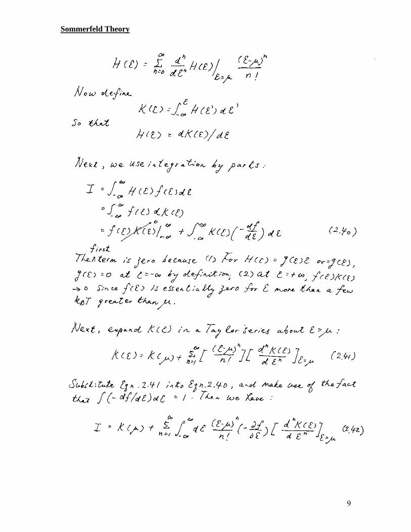
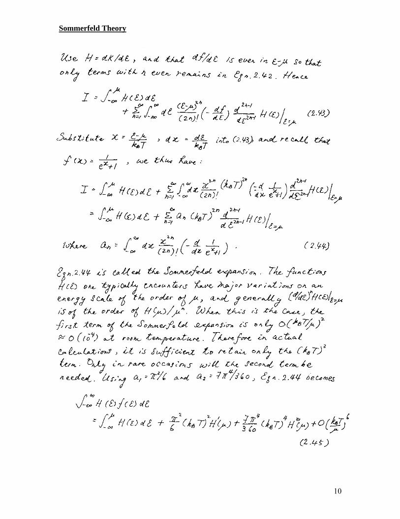
Therefore, the deviation I of the integral, I = dfH

)()( from its zero-temperature

value,

dHF

)( , would be determined by the form of H() near = . If H() does not

vary rapidly in the range (kBT,kBT), I is obtainable, to a good approximation, by replacing H() by its Taylor expansion about = : Continued on next page…

Sommerfeld Theory

9

Sommerfeld Theory

10

s

Sommerfeld Theory

11

Sommerfeld Theory

12

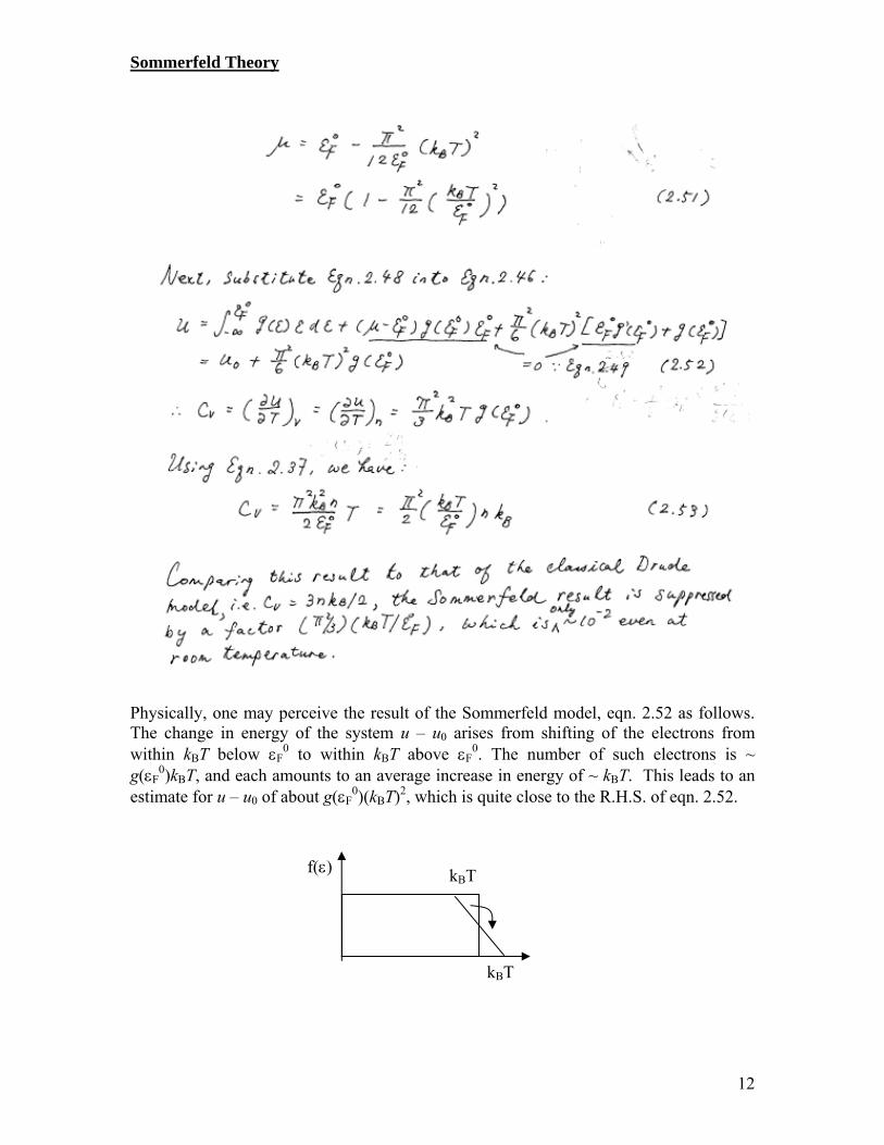
Physically, one may perceive the result of the Sommerfeld model, eqn. 2.52 as follows. The change in energy of the system u – u0 arises from shifting of the electrons from within kBT below F

0 to within kBT above F0. The number of such electrons is ~

g(F0)kBT, and each amounts to an average increase in energy of ~ kBT. This leads to an

estimate for u – u0 of about g(F0)(kBT)2, which is quite close to the R.H.S. of eqn. 2.52.

kBT

kBT f()

Sommerfeld Theory

13

Sommerfeld Theory

14

Sommerfeld Theory

15

2.4 Inadequacy of the Free Electron Model

The Hall Coefficient, RH: Free electron theory predicts RH to be a negative constant = 1/ne, independent of temperature or magnetic field. Although the observed RH agrees in magnitude with this prediction, it is generally dependent on both temperature and magnetic field. In some cases, RH is positive, which is incomprehensible by a free-electron theory.

Why are some elements not metallic? This is the most detrimental challenge to any free-electron model. Why, for example, is boron an insulator while its vertical neighbor in the periodic table, aluminum, an excellent metal? Why is carbon an insulator when the atoms are arranged in the form of diamond but a conductor when the atoms are arranged in the form of graphite? Why are the rare earth metals (characterized by having valence electrons in the 5d orbitals), bismuth and antimony poor conductors?

A major progress can be achieved by accounting for the facts that (1) the

electrons are not free, but interact with the positive ions and additionally the positive ions are arranged periodically in space (as found in experiment). The resulting properties of the electrons – ones that subject to a periodic potential caused by the positive ions - turn out to be not very different from those found in the free electron approximation, except for some modifications to the energy eigen states and energies. This explains why the free-electron models of Drude and Sommerfeld are successful in many ways. Another important change needed concerns the fact that the positive ions are not stationary, but undertake small oscillatory motions whose quantum mechanical analogs are called phonons. Incorporating the resultant lattice dynamics to the consideration brings about much improved prediction of the specific heat capacity. Later we shall also see that a significant improvement to the theory of solids is achieved when we perceive the electron collisions to arise from collisions with the quanta of lattice vibrations, i.e., phonons, rather than the individual ions presumed to be stationary.

Inadequacy of the Free Electron Model

Sommerfeld Theory

16

Ei gi ni

E4 g4 n4

E3 g3 n3

E2 g2 n2

E1 g1 n1

· · · ·

gi: no. of states with energy Ei ni: no. of e- occupying the state Ei

Appendix 2.1 Derivation of the Fermi-Dirac distribution

TSUF

At thermal equilibrium, F is a minimum.

0

i

ii

nn

FF (1)

subject to the constraint that

N =i

in = constant or 0i

in

Since eq. (1) must be satisfied for any combination of

in , we can particularly choose lk nn for two

arbitrary states k and l, while the rest of 0in .

So 0

ll

kk

nn

Fn

n

F

lk n

F

n

F

for arbitrary k and l

in

F chemical potential

i

iiEnU , PkS ln , where P = no. of accessible states = i

iP

For each state i, )!(!

!

ii

ii ngn

gP

1)exp(

1

)exp()1(

/1

/)exp(

ln

ln)ln(ln

))ln()(lnln(

))ln()(lnln(

large is N if lnln

))!ln(!ln!(ln

Tk

Eg

n

g

n

Tk

E

g

n

gn

gn

ng

n

Tk

E

ng

n

Tk

E

n

ngTkEkTngkTnkTkTE

n

F

ngngnnggkTEnF

ngngnnggkS

N-NNN!

ngngkS

B

ii

i

i

i

B

i

i

i

ii

ii

ii

i

B

i

ii

i

B

i

i

iiBiiiii

i

iiiiiiiiiii

iiiiiiiii

iiiii

This probability of occupancy of an energy level (Ei) is commonly referred to as the occupation number.