lecture 35 spectral expansions of source fields|sommerfeld

Lecture 35

Spectral Expansions of SourceFields—Sommerfeld Integrals

In previous lectures, we have assumed plane waves in finding closed form solutions. Planewaves are simple waves, and their reflections off a flat surface or a planarly layered mediumcan be found easily. When we have a source like a point source, it generates a sphericalwave. We do not know how to reflect exactly a spherical wave off a planar interface. Butby expanding a spherical wave in terms of sum of plane waves and evanescennt waves usingFourier transform technique, we can solve for the solution of a point source over a layeredmedium easily in terms of spectral integrals. Sommerfeld was the first person to have donethis, and hence, these integrals are often called Sommerfeld integrals. Finally, we shall applythe method of stationary phase to approximate these integrals to elucidate their physics.From this, we can see ray theory emerging from the complicated mathematics. It remindsme of a lyric from the musical The Sound of Music—Ray, a drop of golden sun! Ray hasmesmerized the human mind, and it will be interesting to see if the mathematics behind it isequally enchanting.

By this time, you probably feel inundated by the ocean of knowledge that you are imbibing.If you can assimilate them, it will be an exhilarating experience.

35.1 Spectral Representations of Sources

A plane wave is a mathematical idealization that does not exist in the real world. In practice,waves are nonplanar in nature as they are generated by finite sources, such as antennasand scatterers: For example, a point source generates a spherical wave which is nonplanar.Fortunately, these waves can be expanded in terms of sum of plane waves. Once this is done,then the study of non-plane-wave reflections from a layered medium becomes routine. In thefollowing, we shall show how waves resulting from a point source can be expanded in terms ofplane waves summation. This topic is found in many textbooks [1,32,35,95,96,181,205,215].

383

384 Electromagnetic Field Theory

35.1.1 A Point Source

There are a number of ways to derive the plane wave expansion of a point source. We willillustrate one of the ways. The spectral decomposition or the plane-wave expansion of thefield due to a point source could be derived using Fourier transform technique. First, noticethat the scalar wave equation with a point source at the origin is(

∇2 + k20

)φ(x, y, z) =

[∂2

∂x2+

∂2

∂y2+

∂2

∂z2+ k2

0

]φ(x, y, z) = −δ(x) δ(y) δ(z). (35.1.1)

The above equation could then be solved in the spherical coordinates, yielding the solutiongiven in the previous lecture, namely, Green’s function with the source point at the origin,or1

φ(x, y, z) = φ(r) =eik0r

4πr. (35.1.2)

The solution is entirely spherically symmetric due to the symmetry of the point source.Next, assuming that the Fourier transform of φ(x, y, z) exists,2 we can write

φ(x, y, z) =1

(2π)3

∞�

−∞

dkxdkydkz φ(kx, ky, kz)eikxx+ikyy+ikzz. (35.1.3)

Then we substitute the above into (35.1.1), after exchanging the order of differentiation andintegration,3 one can simplify the Laplacian operator in the Fourier space, or spectral domain,to arrive at

∇2 =∂2

∂x2+

∂2

∂y2+

∂2

∂z2= −k2

x − k2y − k2

z

Then, together with the Fourier representation of the delta function, which is4

δ(x) δ(y) δ(z) =1

(2π)3

∞�

−∞

dkxdkydkz eikxx+ikyy+ikzz (35.1.4)

we convert (35.1.1) into

∞�

−∞

dkxdkydkz [k20 − k2

x − k2y − k2

z ]φ(kx, ky, kz)eikxx+ikyy+ikzz (35.1.5)

= −∞�

−∞

dkxdkydkz eikxx+ikyy+ikzz. (35.1.6)

1From this point onward, we will adopt the exp(−iωt) time convention to be commensurate with the opticsand physics literatures.

2The Fourier transform of a function f(x) exists if it is absolutely integrable, namely that�∞−∞ |f(x)|dx is

finite (see [110]).3Exchanging the order of differentiation and integration is allowed if the integral converges after the

exchange.4We have made use of that δ(x) = 1/(2π)

�∞−∞ dkx exp(ikxx) three times.

Spectral Expansions of Source Fields—Sommerfeld Integrals 385

Since the above is equal for all x, y, and z, we can Fourier inverse transform the above to get

φ(kx, ky, kz) =−1

k20 − k2

x − k2y − k2

z

. (35.1.7)

Consequently, we have

φ(x, y, z) =−1

(2π)3

∞�

−∞

dkeikxx+ikyy+ikzz

k20 − k2

x − k2y − k2

z

. (35.1.8)

where dk = dkxdkydkz. The above expresses the fact the φ(x, y, z) which is a spherical waveby (35.1.2), is expressed as an integral summation of plane waves. But these plane waves arenot physical plane waves in free space since k2

x + k2y + k2

z 6= k20.

C

Re [kz]

– k20 – k2

x – k2y

⊗

Fourier Inversion Contour

Im [kz]

k20 – k2

x – k2y

×

Figure 35.1: The integration along the real axis is equal to the integration along C plus theresidue of the pole at (k2

0 − k2x − k2

y)1/2, by invoking Jordan’s lemma.

Weyl Identity

To make the plane waves in (35.1.8) into physical plane waves, we have to massage it intoa different form. We rearrage the integrals in (35.1.8) so that the dkz integral is performedfirst. In other words,

φ(r) =1

(2π)3

∞�

−∞

dkxdkyeikxx+ikyy

� ∞−∞

dkzeikzz

k2z − (k2

0 − k2x − k2

y)(35.1.9)

where we have deliberately rearrange the denominator with kz being the variable in the innerintegral. Then the integrand has poles at kz = ±(k2

0 − k2x − k2

y)1/2.5 Moreover, for real k0,and real values of kx and ky, these two poles lie on the real axis, rendering the integral in

5In (35.1.8), the pole is located at k2x + k2

y + k2z = k2

0 . This equation describes a sphere in k space, knownas the Ewald’s sphere [216].


(35.1.8) undefined. However, if a small loss is assumed in k0 such that k0 = k′0 + ik′′0 , thenthe poles are off the real axis (see Figure 35.1), and the integrals in (35.1.8) are well-defined.In actual fact, this is intimately related to the uniqueness principle we have studied before:An infinitesimal loss is needed to guarantee uniqueness in an open space as shall be explainedbelow.

First, the reason is that without loss, |φ(r)| ∼ O(1/r), r → ∞ is not strictly absolutelyintegrable, and hence, its Fourier transform does not exist [52]: The manipulation that leadsto (35.1.8) is not strictly correct. Second, the introduction of a small loss also guarantees theradiation condition and the uniqueness of the solution to (35.1.1), and therefore, the equalityof (35.1.2) and (35.1.8) [35].

Observe that in (35.1.8), when z > 0, the integrand is exponentially small when =m[kz]→∞. Therefore, by Jordan’s lemma [89], the integration for kz over the contour C as shownin Figure 35.1 vanishes. Then, by Cauchy’s theorem [89], the integration over the Fourierinversion contour on the real axis is the same as integrating over the pole singularity locatedat (k2

0 − k2x − k2

y)1/2, yielding the residue of the pole (see Figure 35.1). Consequently, afterdoing the residue evaluation, we have

φ(x, y, z) =i

2(2π)2

∞�

−∞

dkxdkyeikxx+ikyy+ik′zz

k′z, z > 0, (35.1.10)

where k′z = (k20 − k2

x − k2y)1/2 is the value of kz at the pole location.

Similarly, for z < 0, we can add a contour C in the lower-half plane that contributes zeroto the integral, one can deform the contour to pick up the pole contribution. Hence, theintegral is equal to the pole contribution at k′z = −(k2

0 − k2x − k2

y)1/2 (see Figure 35.1). Assuch, the result for all z can be written as

φ(x, y, z) =i

2(2π)2

∞�

−∞

dkxdkyeikxx+ikyy+ik′z|z|

k′z, all z. (35.1.11)

By the uniqueness of the solution to the partial differential equation (35.1.1) satisfyingradiation condition at infinity, we can equate (35.1.2) and (35.1.11), yielding the identity

eik0r

r=

i

2π

∞�

−∞

dkxdkyeikxx+ikyy+ikz|z|

kz, (35.1.12)

where k2x+k2

y+k2z = k2

0, or kz = (k20−k2

x−k2y)1/2. The above is known as the Weyl identity

(Weyl 1919). To ensure the radiation condition, we require that =m[kz] > 0 and <e[kz] > 0over all values of kx and ky in the integration. Furthermore, Equation (35.1.12) could beinterpreted as an integral summation of plane waves propagating in all directions, includingevanescent waves. It is the plane-wave expansion (including evanescent wave) of a sphericalwave.


Figure 35.2: The wave is propagating for kρ vectors inside the disk, while the wave is evanes-cent for kρ outside the disk.

One can also interpret the above as a 2D surface integral in the Fourier space over thekx and ky plane or variables. When k2

x + k2y < k2

0, or the spatial spectrum is inside a diskof radius k0, the waves are propagating waves. But for contributions outside this disk, thewaves are evanescent (see Figure 35.2). And the high Fourier (or spectral) components ofthe Fourier spectrum correspond to evanescent waves. The high spectral components, whichare related to the evanescent waves, are important for reconstructing the singularity of theGreen’s function.

ykρ

aφ x

ρ

Figure 35.3: The kρ and the ρ vector on the xy plane.

Sommerfeld Identity

The Weyl identity has double integral, and hence, is more difficult to integrate numerically.Here, we shall derive the Sommerfeld identity which has only one integral. First, in (35.1.12),we express the integral in cylindrical coordinates and write kρ = xkρ cosα + ykρ sinα, ρ =xρ cosφ + yρ sinφ (see Figure 35.3), and dkxdky = kρdkρ dα. Then, kxx + kyy = kρ · ρ =


kρ cos(α− φ), and with the appropriate change of variables, we have

eik0r

r=

i

2π

∞�

0

kρdkρ

� 2π

0

dαeikρρ cos(α−φ)+ikz|z|

kz, (35.1.13)

where kz = (k20−k2

x−k2y)1/2 = (k2

0−k2ρ)1/2, where in cylindrical coordinates, in the kρ-space,

or the Fourier space, k2ρ = k2

x + k2y. Then, using the integral identity for Bessel functions

given by6

J0(kρρ) =1

2π

2π�

0

dα eikρρ cos(α−φ), (35.1.14)

(35.1.13) becomes

eik0r

r= i

∞�

0

dkρkρkzJ0(kρρ)eikz|z|. (35.1.15)

The above is also known as the Sommerfeld identity (Sommerfeld 1909 [109]; [205][p.242]). Its physical interpretation is that a spherical wave can now be expanded as an integralsummation of conical waves or cylindrical waves in the ρ direction, times a plane wave inthe z direction over all wave numbers kρ. This wave is evanescent in the ±z direction whenkρ > k0.

By using the fact that J0(kρρ) = 1/2[H(1)0 (kρρ) + H

(2)0 (kρρ)], and the reflection formula

that H(1)0 (eiπx) = −H(2)

0 (x), a variation of the above identity can be derived as

eik0r

r=i

2

∞�

−∞

dkρkρkzH

(1)0 (kρρ)eikz|z|. (35.1.16)

–k0•

Im [kρ]

• +k0

SommerfeldIntegration Path

Re [kρ]

Figure 35.4: Sommerfeld integration path.

Since H(1)0 (x) has a logarithmic branch-point singularity at x = 0,7 and kz = (k2

0 − k2ρ)1/2

has algebraic branch-point singularities at kρ = ±k0, the integral in Equation (35.1.16) is

6See Chew [35], or Whitaker and Watson(1927) [217].7H

(1)0 (x) ∼ 2i

πln(x), see Chew [35][p. 14], or Abromawitz or Stegun [117].


undefined unless we stipulate also the path of integration. Hence, a path of integrationadopted by Sommerfeld, which is even good for a lossless medium, is shown in Figure 35.4.Because of the manner in which we have selected the reflection formula for Hankel functions,

i.e., H(1)0 (eiπx) = −H(2)

0 (x), the path of integration should be above the logarithmic branch-point singularity at the origin. With this definition of the Sommerfeld integration, the integralis well defined even when there is no loss, i.e., when the bronach points ±k0 are on the realaxis.

35.2 A Source on Top of a Layered Medium

Previously, we have studied the propagation of plane electromagnetic waves from a singledielectric interface in Section 14.1 as well as through a layered medium in Section 16.1. Itcan be shown that plane waves reflecting from a layered medium can be decomposed intoTE-type plane waves, where Ez = 0, Hz 6= 0, and TM-type plane waves, where Hz = 0,Ez 6= 0.8 One also sees how the field due to a point source can be expanded into plane wavesin Section 35.1.

In view of the above observations, when a point source is on top of a layered medium, itis then best to decompose its field in terms of plane waves of TE-type and TM-type. Then,the nonzero component of Ez characterizes TM waves, while the nonzero component of Hz

characterizes TE waves. Hence, given a field, its TM and TE components can be extractedreadily. Furthermore, if these TM and TE components are expanded in terms of plane waves,their propagations in a layered medium can be studied easily.

The problem of a vertical electric dipole on top of a half space was first solved by Som-merfeld (1909) [109] using Hertzian potentials, which are related to the z components of theelectromagnetic field. The work is later generalized to layered media, as discussed in the liter-ature. Later, Kong (1972) [218] suggested the use of the z components of the electromagneticfield instead of the Hertzian potentials.

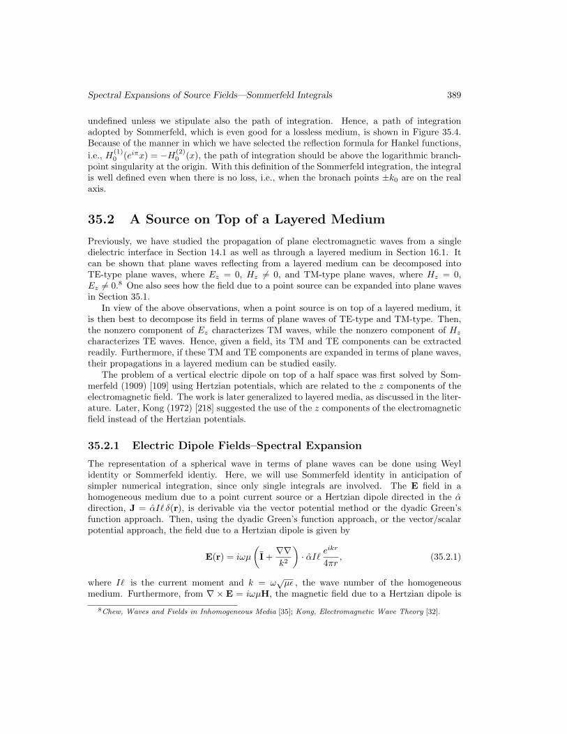
35.2.1 Electric Dipole Fields–Spectral Expansion

The representation of a spherical wave in terms of plane waves can be done using Weylidentity or Sommerfeld identiy. Here, we will use Sommerfeld identity in anticipation ofsimpler numerical integration, since only single integrals are involved. The E field in ahomogeneous medium due to a point current source or a Hertzian dipole directed in the αdirection, J = αI` δ(r), is derivable via the vector potential method or the dyadic Green’sfunction approach. Then, using the dyadic Green’s function approach, or the vector/scalarpotential approach, the field due to a Hertzian dipole is given by

E(r) = iωµ

(I +∇∇k2

)· αI` e

ikr

4πr, (35.2.1)

where I` is the current moment and k = ω√µε , the wave number of the homogeneous

medium. Furthermore, from ∇ × E = iωµH, the magnetic field due to a Hertzian dipole is

8Chew, Waves and Fields in Inhomogeneous Media [35]; Kong, Electromagnetic Wave Theory [32].


shown to be given by

H(r) = ∇× αI` eikr

4πr. (35.2.2)

With the above fields, their TM and TE components can be extracted easily in anticipationof their plane wave expansions for propagation through layered media.

(a) Vertical Electric Dipole (VED)

Region 1

Region i

z

x

–d1

–di

Figure 35.5: A vertical electric dipole over a layered medium.

A vertical electric dipole shown in Figure 35.5 has α = z; hence, in anticipation of their planewave expansions, the TM component of the field is characterized by Ez 6= 0 or that

Ez =iωµI`

4πk2

(k2 +

∂2

∂z2

)eikr

r, (35.2.3)

and the TE component of the field is characterized by

Hz = 0, (35.2.4)

implying the absence of the TE field.Next, using the Sommerfeld identity (35.1.16) in the above, and after exchanging the order

of integration and differentiation, we have9

Ez =−I`4πωε

∞�

0

dkρk3ρ

kzJ0(kρρ)eikz|z|, |z| 6= 0 (35.2.5)

after noting that k2ρ + k2

z = k2. Notice that now Equation (35.2.5) expands the z componentof the electric field in terms of cylindrical waves in the ρ direction and a plane wave in the zdirection. Since cylindrical waves actually are linear superpositions of plane waves, becausewe can work backward from (35.1.16) to (35.1.12) to see this. As such, the integrand in

9By using (35.1.16) in (35.2.3), the ∂2/∂z2 operating on eikz |z| produces a Dirac delta function singularity.Detail discussion on this can be found in the chapter on dyadic Green’s function in Chew, Waves and Fieldsin Inhomogeneous Media [35].


(35.2.5) in fact consists of a linear superposition of TM-type plane waves. The above is alsothe primary field generated by the source.10

Consequently, for a VED on top of a stratified medium as shown, the downgoing planewave from the point source will be reflected like TM waves with the generalized reflectioncoefficient RTM12 . Hence, over a stratified medium, the field in region 1 can be written as

E1z =−I`

4πωε1

∞�

0

dkρk3ρ

k1zJ0(kρρ)

[eik1z|z| + RTM12 eik1zz+2ik1zd1

], (35.2.6)

where k1z = (k21 − k2

ρ)12 , and k2

1 = ω2µ1ε1, the wave number in region 1.

The phase-matching condition dictates that the transverse variation of the field in all theregions must be the same. Consequently, in the i-th region, the solution becomes

εiEiz =−I`4πω

∞�

0

dkρk3ρ

k1zJ0(kρρ)Ai

[e−ikizz + RTMi,i+1e

ikizz+2ikizdi]. (35.2.7)

Notice that Equation (35.2.7) is now expressed in terms of εiEiz because εiEiz reflects andtransmits like Hiy, the transverse component of the magnetic field or TM waves.11 Therefore,

RTMi,i+1 and Ai could be obtained using the methods discussed in Chew, Waves and Fields inInhomogeneous Media [110].

This completes the derivation of the integral representation of the electric field everywherein the stratified medium. These integrals are known as Sommerfeld integrals. The casewhen the source is embedded in a layered medium can be derived similarly.

(b) Horizontal Electric Dipole (HED)

The HED is more complicated. Unlike the VED that excites only the TM waves, an HED willexcite both TE and TM waves. For a horizontal electric dipole pointing in the x direction,α = x; hence, (35.2.1) and (35.2.2) give the TM and the TE components, in anticipation oftheir plane wave expansions, as

Ez =iI`

4πωε

∂2

∂z∂x

eikr

r, (35.2.8)

Hz = − I`4π

∂

∂y

eikr

r. (35.2.9)

10One can perform a sanity check on the odd and even symmetry of the fields’ z-component by sketchingthe fields of a static horizontal electric dipole.

11See Chew, Waves and Fields in Inhomogeneous Media [35], p. 46, (2.1.6) and (2.1.7). Or we can gatherfrom (14.1.6) to (14.1.7) that the µiHiz transmits like Eiy at a dielectric interface, and by duality, εiEiztransmits like Hiy .


Then, with the Sommerfeld identity (35.1.16), we can expand the above as

Ez = ± iI`

4πωεcosφ

∞�

0

dkρ k2ρJ1(kρρ)eikz|z| (35.2.10)

Hz = iI`

4πsinφ

∞�

0

dkρk2ρ

kzJ1(kρρ)eikz|z|. (35.2.11)

Now, Equation (35.2.10) represents the wave expansion of the TM field, while (35.2.11) repre-sents the wave expansion of the TE field in terms of Sommerfeld integrals which are plane-waveexpansions in disguise. Observe that because Ez is odd about z = 0 in (35.2.10), the down-going wave has an opposite sign from the upgoing wave. At this point, the above are just theprimary field generated by the source.

On top of a stratified medium, the downgoing wave is reflected accordingly, depending onits wave type. Consequently, we have

E1z =iI`

4πωε1cosφ

∞�

0

dkρ k2ρJ1(kρρ)

[±eik1z|z| − RTM12 eik1z(z+2d1)

], (35.2.12)

H1z =iI`

4πsinφ

∞�

0

dkρk2ρ

k1zJ1(kρρ)

[eik1z|z| + RTE12 e

ik1z(z+2d1)]. (35.2.13)

Notice that the negative sign in front of RTM12 in (35.2.12) follows because the downgoingwave in the primary field has a negative sign as shown in (35.2.10).

35.3 Stationary Phase Method—Fermat’s Principle

Sommerfeld integrals are rather complex, and by themselves, they do not offer much physicalinsight into the physics of the field. To elucidate the physics, we can apply the stationaryphase method to find approximations of these integrals when the frequency is high, or kr islarge, or the observation point is many wavelengths away from the source point. It turns outthat this method is initmately related to Fermat’s principle.

In order to avoid having to work with special functions like Bessel functions, we convertthe Sommerfeld integrals back to spectral integrals in the cartesian coordinates. We couldhave obtained the aforementioned integrals in cartesian coordinates were we to start with theWeyl identity instead of the Sommerfeld identity. To do the back conversion, we make use ofthe identity,

eik0r

r=

i

2π

∞�

−∞

dkxdkyeikxx+ikyy+ikz|z|

kz= i

∞�

0

dkρkρkzJ0(kρρ)eikz|z|. (35.3.1)


We can just focus our attention on the reflected wave term in (35.2.6) and rewrite it incartesian coordinates to get

ER1z =−I`

8π2ωε1

∞�

−∞

dkxdkyk2x + k2

y

k1zRTM12 eikxx+ikyy+ik1z(z+2d1)

=

∞�

−∞

dkxdky1

k1zF (kx, ky)eikxx+ikyy+ik1z(z+2d1) (35.3.2)

where

F (kx, ky) =−I`

8π2ωε1(k2x + k2

y)RTM12

In the above, k2x+k2

y+k21z = k2

1 is the dispersion relation satisfied by the plane wave in region

1. Also, RTM12 is dependent on kiz =√k2i − k2

x − k2y in cartesian coordinates, where i = 1, 2.

Now the problem reduces to finding the approximation of the following integral:

ER1z =

∞�

−∞

dkxdky1

k1zF (kx, ky)eirh(kx,ky) (35.3.3)

where

rh(kx, ky) = r(kxx

r+ ky

y

r+ k1z

z

r

), (35.3.4)

We want to approximate the above integral when kr is large. For simplicity, we have setd1 = 0 to begin with.


Figure 35.6: In this figure, t can represent kx or ky when one of them is varying. Aroundthe stationary phase point, the function h(t) is slowly varying. In this figure, λ = r, andg(kx, ky, λ) = eiλh(kx,ky) = eirh(kx,ky). When λ = r is large, the function g(λ, kx, ky) israpidly varying with respect to either kx or ky. Hence, most of the contributions to theintegral comes from around the stationary phase point.

In the above, eirh(kx,ky) is a rapidly varying function of kx and ky when x, y, and z arelarge, or r is large compared to wavelength.12 In other words, a small change in kx or kywill cause a large change in the phase of the integrand, or the integrand will be a rapidlyvarying function of kx and ky. Due to the cancellation of the integral when one integratesa rapidly varying function, most of the contributions to the integral will come from aroundthe stationary point of h(kx, ky) or where the function is least slowly varying. Otherwise,the integrand is rapidly varying away from this point, and the integration will destructivelycancel with each other, while around the stationary point, they will add constructively.

The stationary point in the kx and ky plane is found by setting the derivatives of h(kx, ky)with respect to to kx and ky to zero. By so doing

∂h

∂kx=x

r− kxk1z

z

r= 0,

∂h

∂ky=y

r− kyk1z

z

r= 0 (35.3.5)

The above represents two equations from which the two unknowns, kxs and kys, at thestationary phase point can be solved for. By expressing the above in spherical coordinates,x = r sin θ cosφ, y = r sin θ sinφ, z = r cos θ, the values of (kxs, kys), that satisfy the aboveequations are

kxs = k1 sin θ cosφ, kys = k1 sin θ sinφ (35.3.6)

with the corresponding k1zs = k1 cos θ.

12The yardstick in wave physics is always wavelength. Large distance is also synonymous to increasing thefrequency or reducing the wavelength.


When one integrates on the kx and ky plane, the dominant contribution to the integral willcome from the point in the vicinity of (kxs, kys). Assuming that F (kx, ky) is slowly varying,we can equate F (kx, ky) to a constant equal to its value at the stationary phase point, andsay that

ER1z ' F (kxs, kys)

∞�

−∞

1

k1zeikxx+ikyy+ik1zzdkxdky = 2πF (kxs, kys)

eik1r

ir(35.3.7)

In the above, the integral can be performed in closed form using the Weyl identity. The aboveexpression has two important physical interpretations.

(i) Even though a source is emanating plane waves in all directions in accordance to(35.1.12), at the observation point r far away from the source point, only one or fewplane waves in the vicinity of the stationary phase point are important. They interferewith each other constructively to form a spherical wave that represents the ray connect-ing the source point to the observation point. Plane waves in other directions interferewith each other destructively, and are not important. That is the reason that the sourcepoint and the observation point is connected only by one ray, or one bundle of planewaves in the vicinity of the stationary phase point. These bundle of plane waves arealso almost paraxial with respect to each other.

(ii) The function F (kx, ky) could be a very complicated function like the reflection coefficientRTM , but only its value at the stationary phase point matters. If we were to make d1 6= 0again in the above analysis, the math remains similar except that now, we replace rwith rI =

√x2 + y2 + (z + 2d1)2. Due to the reflecting half-space, the source point

has an image point as shown in Figure 35.7 This physical picture is shown in the figurewhere rI now is the distance of the observation point to the image point. The stationaryphase method extract a ray that emanates from the source point, bounces off the half-space, and the reflected ray reaches the observer modulated by the reflection coefficientRTM . But the value of the reflection coefficient that matters is at the angle at whichthe incident ray impinges on the half-space.

(iii) At the stationary point, the ray is formed by the k-vector where k = xk1 sin θ cosφ +yk1 sin θ sinφ + zk1 cos theta. This ray points in the same direction as the positionvector of the observation point r = xr sin θ cosφ+ yr sin θ sinφ+ zr cos theta. In otherwords, the k-vector and the r-vector point in the same direction. This is reminiscentof Fermat principle, because when this happens, the ray propagates with the minimumphase between the source point and the observation point. When z → z + 2d1, theray for the image source is altered to that shown in Figure 35.7 where it the ray isminimum phase from the image source to the obervation point. Hence, the stationaryphase method is initimately related to Fermat’s principle.


Figure 35.7: At high frequencies, the source point and the observation point are connectedby a ray. The ray represents a bundle of plane waves that interfere constructively. This eventrue for a bundle of plane waves that reflect off an interface. So ray theory or ray opticsprevails here, and the ray bounces off the interface according to the reflection coefficient of aplane wave impinging at the interface with θI .

35.4 Riemann Sheets and Branch Cuts13

The Sommerfeld integrals will have integrands that are multi-value or double value. Properbook keeping is needed so that the evaluation of these integrals can be performed unambigu-ously. The function kz = (k2

0 − k2ρ)1/2 in (35.1.15) and (35.1.16) are double-value functions

because, in taking the square root of a number, two values are possible. In particular, kz isa double-value function of kρ. Consequently, for every point on a complex kρ plane in Figure35.4, there are two possible values of kz. Therefore, as an example, the integral (35.1.11)is undefined unless we stipulate which of the two values of kz is adopted in performing theintegration.

A multivalue function is denoted on a complex plane with the help of Riemann sheets[35, 89]. For instance, a double-value function such as kz is assigned two Riemann sheets toa single complex plane. On one of these Riemann sheets, kz assumes a value just opposite insign to the value on the other Riemann sheet. The correct sign for kz is to pick the squareroot solution so that =m(kz) > 0. This will ensure a decaying wave from the source.

35.5 Some Remarks14

Even though we have arrived at the solutions of a point source on top of a layered mediumby heuristic arguments of plane waves propagating through layered media, they can alsobe derived more rigorously. For example, Equation (35.2.6) can be arrived at by matchingboundary conditions at every interface. The reason why a more heuristic argument is stillvalid is due to the completeness of Fourier transforms. It is best explained by putting a sourceover a half space and a scalar problem.

13This may be skipped on first reading.14This may be skipped on first reading.


We can expand the scalar field in the upper region as

Φ1(x, y, z) =

∞�

−∞

dkxdkyΦ1(kx, ky, z)eikxx+ikyy (35.5.1)

and the scalar field in the lower region as

Φ2(x, y, z) =

∞�

−∞

dkxdkyΦ2(kx, ky, z)eikxx+ikyy (35.5.2)

If we require that the two fields be equal to each other at z = 0, then we have

∞�

−∞

dkxdkyΦ1(kx, ky, z = 0)eikxx+ikyy =

∞�

−∞

dkxdkyΦ2(kx, ky, z = 0)eikxx+ikyy (35.5.3)

In order to remove the integral, and replace it with a simple scalar problem, one has to imposethe above equation for all x and y. Then by the completeness of Fourier transform impliesthat15

Φ1(kx, ky, z = 0) = Φ2(kx, ky, z = 0) (35.5.4)

The above equation is much simpler than that in (35.5.3). In other words, due to the com-pleteness of Fourier transform, one can match a boundary condition spectral-component byspectral-component. If the boundary condition is matched for all spectral components, than(35.5.3) is also true.

15Or that we can perform a Fourier inversion on the above integrals.

lecture 35 spectral expansions of source fields|sommerfeld

Documents