Sample-Based Estimation of Bicycle Miles of Travel

(BMT)

2001-23 Final Report

Res

earc

h

Technical Report Documentation Page

1. Report No. 2. 3. Recipients Accession No. MN/RC – 2001-23 4. Title and Subtitle 5. Report Date

October 2001 6.

SAMPLE-BASED ESTIMATION OF BICYCLE MILES OF TRAVEL (BMT)

7. Author(s) 8. Performing Organization Report No. Gary A. Davis, Ph.D. and Trina Wicklatz, BLA/MLA 9. Performing Organization Name and Address 10. Project/Task/Work Unit No.

11. Contract (C) or Grant (G) No.

University of Minnesota Dept. of Civil Engineering 500 Pillsbury Drive S.E. Minneapolis, MN 55455-0116

C) 74708 wo) 36

12. Sponsoring Organization Name and Address 13. Type of Report and Period Covered Final Report 14. Sponsoring Agency Code

Minnesota Department of Transportation 395 John Ireland Boulevard Mail Stop 330 St. Paul, Minnesota 55155 15. Supplementary Notes 16. Abstract (Limit: 200 words)

This project provides a statistically defensible estimate of bicycle-miles of travel (BMT) for at a least substantial portion of the Twin Cities region and assesses the feasibility of monitoring bicycle volumes using sampling methods similar to those used to monitor motor vehicle traffic. Researchers used an ArcView database of the Twin Cities street system for the initial sampling frame and extended the database by manually adding information about average annual daily traffic volumes and about on- and off-road bicycle facilities. A stratified random sample of roadways links in Hennepin, Ramsey, and Dakota counties was drawn, and during the months of May through June and August through October 1998, the daytime bicycle volume for one day at each sampled site was obtained using time-lapse video. Researchers then used Cochrane’s “combined” estimator to compute an estimate of average daytime BMT for the study area.

17. Document Analysis/Descriptors 18. Availability Statement Bicycle monitoring Bicycle-miles of travel BMT GIS

Traffic sampling Vehicle-miles of travel Bike lane

No restrictions. Document available from: National Technical Information Services, Springfield, Virginia 22161

19. Security Class (this report) 20. Security Class (this page) 21. No. of Pages 22. Price Unclassified Unclassified

101

Sample Based Estimation of

Bicycle Miles of Travel (BMT)

Final Report

Prepared by: Gary A. Davis, Ph.D.

Trina Wicklatz, BLA/MLA

Department of Civil Engineering University of Minnesota Minneapolis MN 55455

October 2001

Published by:

Minnesota Department of Transportation Office of Research Services 395 John Ireland Boulevard

Mail Stop 330 St Paul, Minnesota 55155

The contents of this report reflect the views of the authors who are responsible for the facts and accuracy of

the data presented herein. The contents do not necessarily reflect the views or policies of the Minnesota Department of Transportation. This report does not constitute a standard, specification, or regulation.

The authors and the Minnesota Department of Transportation do not endorse products or manufacturers. Trade or manufacturers’ names appear herein solely because they are considered essential to this report.

ACKNOWLEDGEMENTS

The authors would like to acknowledge graduate student Kate Sanderson, and

undergraduate research assistants Chris Hager, Jesse Struve and Andrea Swansby for their

contribution to the project. Special recognition goes to Jim Gaylord who went the extra mile in

helping us bring in the data.

The authors express appreciation to all whose cooperation made it possible for us to

collect the bicycle count data including: all communities, counties and regional park systems who

gave their permission to videotape in their jurisdiction; Northern States Power Company; ATD

Northwest; and the Real Estate Office and the Human Subjects Committee at the University of

Minnesota.

i

Table of Contents

CHAPTER 1 INTRODUCTION 1

CHAPTER 2 LITERATURE REVIEW 3

CHAPTER 3 SAMPLING METHODS 5

3.1. Overview 8

3.2. Sampling Procedures 9

3.3. Bicycle Facility Types 12

3.4. Geographic Subareas 19

3.5. Study Characteristics 28

3.6. Data Collection 29

3.6.1. Overview and Checklist 29

3.6.2. GIS Database 30

3.6.3. Sample Selection 35

3.6.4. Count Program 36

3.6.5. Counting Guidelines 41

3.6.6. Scheduling and Management 42

CHAPTER 4 COMPUTING ESTIMATES OF BMT 47

4.1. Estimating Average Daytime BMT 47

4.2. Sample Size Selection 51

4.3. Annual Expansion of BMT Estimates 52

ii

CHAPTER 5 SUMMARY AND CONCLUSIONS 55

APPENDIX A METADATA FOR BICYCLE FACILITIES 57

APPENDIX B PROJECT MANAGEMENT FORMS 63

B-1. General Permission Form 64

B-2. Explanatory Label 65

B-3. Master Key 66

B-4. Master Site Selection Sheet 67

B-5. Examples of Site Sheets and Site Maps 70

B-6. Installation Sheet 74

B-7. Count Sheet 76

APPENDIX C POWER COMPANY REQUIREMENTS 79

APPENDIX D PROTECTION OF HUMAN SUBJECTS 81

APPENDIX E BICYCLE COUNTS AND LOCATIONS 83

iii

List of Figures

Figure 1. Three County Study Area 7

Figure 2. Bicycle Facilities by Type in the 3-County Metro Area 13

Figure 3. Geographic Subareas 18

Figure 4. Patterns and Densities – On-Road & Off-Road Bicycle Facilities 21

Figure 5. Patterns and Densities - Roadways 22

Figure 6. Pattern and Density Samples – Urban and Suburban Roadways 24

Figure 7. Suburban Connectivity – Bicycle and Roadway Systems 26

Figure 8. Roadway Anomalies not included in the Study 32

Figure 9. Counted Sites 34

List of Tables

Table 1. Numbers of Segments by Facility Type, Subarea and County 28

Table 2. Total BMT on Sampled Links, in each Sample Stratum 48

Table 3. Total Mileage of Sampled Links in each Sample Stratum 48

Table 4. Total Mileage in Study Area in each Sample Stratum 49

Table 5. Estimated Daytime Daily BMT in Each Sample Stratum 49

Table 6. Estimated Day-of-Week Factors from Parkway Bicycle Detector 54

Table 7. Estimated Monthly Factors from Parkway Bicycle Detector 54

EXECUTIVE SUMMARY

This project was undertaken to (1) provide a statistically defensible estimate of bicycle -

miles of travel for at least a substantial portion of the Twin Cities region, and (2) to assess the

feasibility of monitoring bicycle volumes using sampling methods similar to those employed to

monitor vehicle traffic volumes. An ArcView database of the Twin Cities street system developed

by The Lawrence Group provided the initial sampling frame, and this was extended by manually

adding information on average annual daily traffic volumes, and about on- and off-road bicycle

facilities. Because of time and resource constraints, the extended data base could be developed

only for Hennepin, Ramsey and Dakota counties, so these three counties comprised the project’s

study area. A stratified random sample of roadway links was then developed for the study area,

where each combination of four roadway link types, and four geographical subareas, made up the

sample strata. During the months of May-June, and August-October 1998, the daytime (7 AM to

7 PM) bicycle volume for one day at each sampled site was obtained by first recording the traffic

activity on videotape and then manually counting bicycles. Cochrane’s “combined” ratio

estimator was then used to compute an estimate of average daytime BMT in the study area

(383754 bicycle-miles/day) and the estimate’s standard error (69994 bicycle -miles/day).

Estimates of future sample sizes needed to achieve given levels of precision were also computed,

as well as estimates of annual BMT for the study area, and the entire metro area.

1

Chapter 1 INTRODUCTION

In 1976, Orhn estimated that purposeful trip making by bicycle in the Twin Cities could

potentially draw more users per day than the bus system.1 And for at least 20 years, it has been

argued that an increased use of bicycles for purposeful trip making could help lessen urban traffic

congestion and have a positive effect on congestion-produced air pollution and energy

consumption. However, estimates of actual bicycle usage, expressed either as trips or as bicycle

miles of travel (BMT), have never been available.

More recently, the Minnesota Comprehensive State Bicycle Plan calls for “…bicycle

miles traveled to reach a growth rate of 10% per year”2 by 1999. This goal leads to the problem

of developing objective methods for estimating total use, so that growth rate can be measured or

more objectively estimated. In fact, program recommendations in the State Bicycle Plan also

state, “that statistics on bicycle use and accident rates per mile traveled be maintained in such a

way that they are comparable with those for motor vehicles, and are integral parts of

transportation information systems.”3

The problem of developing an estimate for Bicycle Miles of Travel (BMT) has never

been addressed. However, an analogous problem is the development of estimations of Vehicle

Miles of Travel (VMT) using a limited number of vehicle counts. The Federal Highway

Administration (FHWA) has published several documents describing how such estimations for

VMT can be accomplished.4 This project used these methods, particularly those described in

Guide to Urban Traffic Volume Counting (1975), along with bicycle count data gathered by the

project. Regarding the use of estimation procedures, the guide comments:

The most desirable method for determining urban VMT … would be to make

representative traffic counts on every section of urban street. This of course, would result in

extremely expensive counting programs and would be practical only in cities which make

extensive counts for traffic engineering purposes. Accordingly, probability sampling procedures

were developed to provide a cost-effective basis for estimating VMT on urban streets and

highways.5

The primary objective of this project was to compute a sample -based estimate of BMT on

a network of bikeways and roadways in the Twin Cities region. This involved the mapping and

development of a (GIS) database describing the bikeway and roadway network and obtaining

2

single-day bicycle volume counts on a sample of network links using videotape traffic counting

technology. The program sample organized bikeways and roadways into four distinct facility

types and divided the Twin Cities area into four subareas having “homogenous bicycle use” (as

described in Chapter 2).

A secondary objective, implicit in a project that addresses a new topic of inquiry, is the

objective of learning more about the methodology employed. This study developed or uncovered

methodological details regarding sample program design, data collection and sample sizes needed

to guarantee BMT estimates with a specified level of precision.

The report is organized as follows:

• Chapter 2 gives a context for the study and a context for the methodology employed

by the project by reviewing the literature on the subject;

• Chapter 2 describes the project’s sample program design, along with data collection

and BMT estimation methodologies;

• Chapter 4 provides the estimate for BMT;

• Chapter 5 provides recommendations and commentary.

The appendices provide the following information:

• Appendix A describes the metadata this project developed for bicycle facilities and

added to the Metropolitan Council’s street centerline database for Dakota, Hennepin,

and Ramsey counties;

• Appendix B provides the forms developed for managing the bicycle count;

• Appendix C describes the local power company’s installation requirements placing

the video equipment on power company poles;

• Appendix D briefly discusses the policy of the University of Minnesota and the

policy of the federal government regarding the observation of public behavior and

gives websites for more detailed information;

• Appendix E contains tables providing the bicycle counts taken at the randomly

selected locations in the study area, along with characteristics of the locations such as

bicycle facility type and the Average Daily Traffic (ADT) for motor vehicles on the

selected roadways.

3

Chapter 2 LITERATURE REVIEW

Although the project’s literature search failed to turn up papers or reports in which

region-wide BMT had been estimated, there are two related lines of work: one addressing the

estimation of vehicle miles of travel (VMT), and the other dealing with patterns of variation in

bicycle traffic volumes.

In a report prepared for the Federal Highway Administration (FHWA), Ferlis, Bowman

and Cima 6 presented a formula for estimating regionwide VMT from traffic counts collected on a

sample of roadway locations along with detailed instructions on how to develop the sample

program. Although the sample development procedures described in this report are sound, the

VMT estimation formula suffers from technical inadequacies. The report was to be an update and

extension of an earlier report prepared by FHWA, The Preliminary Guide to Urban Traffic

Volume Counting (hereafter, referred to as the GUTVC)7.

The GUTVC describes two procedures, a basic approach and an alternate approach, for

estimating region-wide VMT from a sample of traffic counts, where the estimation formulas were

taken from well-known texts on sampling. 8, 9 The GUTVC also recommends basic sample

program design and describes how to estimate the minimum sample size that will give VMT

estimates with some desired precision.

For the basic approach, coefficients of variation describing the temporal and spatial

variability of vehicle volumes, together with the average length of the roadway segments making

up the population, must be known beforehand. A ratio estimator of average VMT per mile is then

multiplied by the total mileage of population in order to estimate total VMT. This method also is

implicitly recommended in the Traffic Monitoring Guide10. For the alternate approach, the

average and the standard deviation of the lengths of the roadway segments making up the

population must be known. Average VMT per segment is multiplied by the total number of

segments in the population to estimate total VMT. The authors of the GUTVC recommend using

the alternate approach when the required link length statistics are available and Hoang and

Poteat11 describe using the alternate method to estimate statewide VMT in Florida.

Using Geographic Information System (GIS) software such as Arc View from ESRI

Corp., segment length statistics are easily obtained once a network of roadways and bicycle

facilities has been mapped and represented in a database. The other inputs required for estimating

4

the sample size, mean daily volume and the variance in daily volumes across time and across

segments, can only be determined by counting bicycles.

The research dealing with patterns of variation in bicycle traffic volumes is scant.

Buckley12 described a bicycle counting program conducted in Boston and reported that bicycle

traffic volumes 1) appeared to grow over a six-year period, and 2) showed significant seasonal

and weather-related variation patterns. Estimates of BMT were not reported, and the data

reported in this paper were not sufficient to compute estimates of either temporal or spatial

variation in bicycle volume. Hunter and Huang13 reviewed bicycle counts on trails and paths

reported by a number of different cities in the U.S., and showed examples of peak-hour counts of

100 bicycles/hour and daily volumes of 400-1200 bicycles/day. Once again, estimates of BMT

were not reported and the information this paper provided was not sufficient to estimate temporal

or spatial coefficients of variation. Niemeier14 described morning and afternoon peak period

counts conducted in Seattle across an entire year. The data in Niemeier’s Table 2 show temporal

coefficients of variation ranging between 37% and 72% for the morning peak volume at four sites

in Seattle. Using this data, it is possible to compute a spatial coefficient of variation equal to

68%. Estimates of BMT were not reported.

If temporal and spatial coefficients of variation equal to 60% are taken as being typical

of daily bicycle traffic, then it is possible to use formula #5 in the GUTVC15 to estimate a bicycle

count sample size for planning purposes. In particular, if we want to estimate region-wide BMT

with a 10% accuracy and 68% confidence, we would need to count about 72 miles of segments.

Assuming each segment is ½ mile long, then about 144 segments should be included in the

sample. (The project actually measured 160 segments.)

5

Chapter 3 SAMPLING METHODS

Since there has been little to no rigorous collection and modeling of data related to

bicycle use, the project could not rely on previous research to provide it with any kind of

methodology, especially with respect to understanding various parameters of bicycle use. For

most of this century, transportation research has developed fundamental knowledge regarding

travel behavior for motor vehicle transportation and transportation modeling relies today on this

primary material. This wealth of understanding and background does not exist for bicycle

transportation. Basic questions regarding vehicle use that can be answered in the world of the

motor vehicle remain unanswered in any research or modeling procedures involving bicycle

transportation.

With this situation, it was necessary for project personnel to use available information

and their collective knowledge and understanding of the study area and bicycling as

transportation planners, long-time area residents and cyclists. This was particularly true when

characteristics of the sample were developed as discussed in sections 3.3 and 3.4.

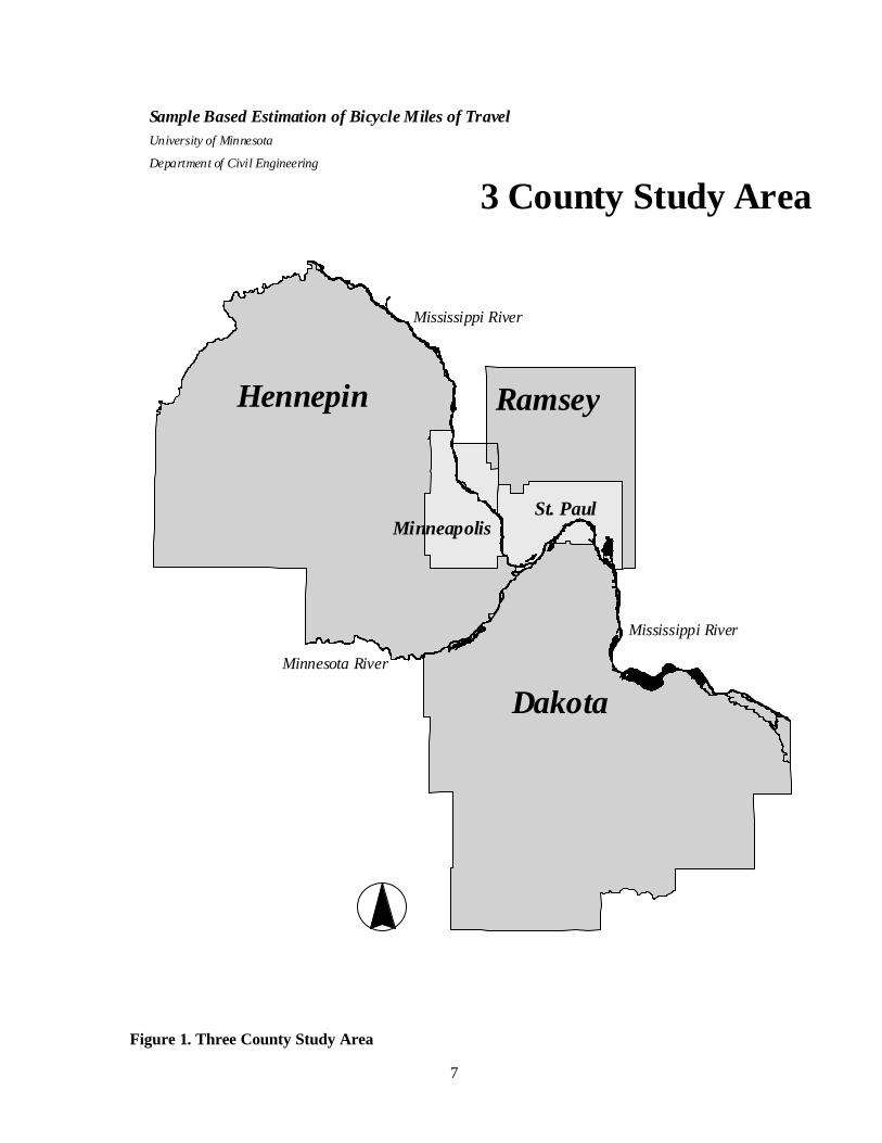
The project used video technology to count cyclists in three counties in the Twin Cities

metropolitan area (Figure 1). Though video technology has been used before in transportation, to

our knowledge it was never used on a project of this type and scope. In addition, the project

discovered a number of unexpected aspects of the data collection process that needed to be

addressed in order for any data to be collected at all. All of these aspects of the BMT research are

discussed in this chapter as follows:

• The overview in section 3.1 provides a quick description of the sampling program

used in this research;

• Section 3.2 describes the sample program recommendations given in the Guide to

Urban Traffic Volume Counting,16 published by the USDOT and FHWA, for

developing estimates for (motor) vehicle miles of travel (VMT) using a limited

number of vehicle counts;

• Sections 3.3 and 3.4 define and discuss in detail the bicycle facility types and the

geographic subareas developed for the BMT sample program;

• Section 3.5 provides an assortment of study characteristics including when the counts

were taken, weather, topography and a table of the total number of segments of each

facility type in each subarea and county;

6

• Section 3.6 opens with an overview in checklist format of the more detailed

subsections that follow it, all describing various necessary or recommended steps to

be taken during the data collection phase.

7

Dakota

Hennepin Ramsey

Mississippi River

Minnesota River

Mississippi River

MinneapolisSt. Paul

Sample Based Estimation of Bicycle Miles of TravelUniversity of Minnesota

Department of Civil Engineering

3 County Study Area

Figure 1. Three County Study Area

8

3.1. Overview

This section provides a quick overview of the sampling program’s bicycle facility types

and geographic subareas for easy reference. More detail and discussion on the information

included here is found in sections 3.3 and 3.4.

Bicycle Facility Types

The BMT project established four basic facility types for measuring bicycle use:

• Off-road bicycle facilities Off-road bicycle facilities are physically separated from roadway space for motor vehicles and include bicycle facilities in parks and alongside roadways.

• On-road bicycle facilities On-road bicycle facilities are physically marked within a street or roadway that is used by motor vehicles and includes all striped bicycle facilities.

• Roadways with motor vehicle ADT <5000 And with no bicycle facilities This category defines smaller and quieter streets and consists mostly of local or residential streets.

• Roadways with motor vehicle ADT ≥5000 (Average Annual Daily Traffic, AADT) And with no bicycle facilities This category defines larger and busier streets and consists mostly of arterials and collectors.

Geographic Subareas

The project established the following four subareas with the following characteristics:

• Urban Highest density of roadways Grid street system High connectivity of existing streets and roadways Overall, medium to sparse density of bicycle facilities

• Suburban Medium density of roadways Non-grid, street patterns; many culs-de-sac and eyebrow street types Lower connectivity of existing streets and roadways, many dead-ends Dense bicycle system

• Rural Low density of roadways Grid roadways follow section lines, small towns High connectivity of existing streets and roadways Very sparse bicycle system

9

• University of Minnesota

(The area is described by a radius approximately 1 mile from the University of Minnesota’s East Bank and West Bank campuses in Minneapolis)

Has characteristics of the urban subarea Medium density of bicycle facilities Observations, together with previous counts and surveys show a high bicycle mode share around this U of M campus and therefore, a separately identifiable homogenous zone of bicycle use.17

3.2. Sampling Procedures

The Guide to Urban Traffic Volume Counting (GUTVC) describes statistical procedures

for urban traffic counting programs and sets forth sampling guidelines to be used in developing

estimates for traffic volumes and vehicle miles of travel. In general, their guidelines note:

• A street link is assumed to be a designated section of street with relatively homogeneous volumes …

• A “link-day” is a 24-hour [count] period for a given link. This procedure will allow sampling links and days separately. 18

Any measurement of vehicle miles of travel requires counting vehicles on a “segment”

(also called a “link”) of roadway. A segment is defined to be a length of roadway with similar

traffic characteristics (i.e., with “homogenous” volumes). In motor vehicle networks, the

boundaries of a segment are typically street intersections, exit/entrance ramps, or entries to

parking lots of major destinations. However, the definition of the segments in any bicycle

network is at a finer granularity than in the motor vehicle network. This is because the bicycle is

smaller, more maneuverable and flexible than the motor vehicle, making it possible for bicyclists

to enter a segment in the system at locations in addition to those that are typically recognized as

‘formal’ entries to a segment by motor vehicles. Determining all entries for bicyclists to all of the

segments in a system is impossible at present and will probably remain so because of the

bicycle’s extreme maneuverability and flexibility.

Therefore, for the BMT project, entry to segments in the system used by cyclists is

defined:

• On streets and roadways, as that which is defined for motor vehicles and

• On off-road bicycle facilities, as intersections that can be seen on maps or aerial

photos of the off-road bicycle facilities.

10

The GUTVC continues by recommending that the following steps be used in developing

a sampling program (for modeling motor vehicle use).

1. Establish Geographic Sub-Areas – The urban area should be subdivided into the analysis units for which specific information is desired. A small urban area (population under 250,000) would probably be subdivided into 2 or 3 divisions which distinguish between central city and suburbs…. Larger urban areas (population over 1,000,000) could be subdivided into 5 to 7 sub-areas…. The location of rings and sectors should be judiciously selected to correlate with common growth areas. It should be noted that total number of samples required increases significantly as stratifications increase.

2. Functionally Classify Streets – The streets in each sub-area should be functionally

classified. In order to keep the required sample at a manageable size, the number of functional classes should be limited. The following scheme is recommended:

a) Local streets;

b) Arterial streets (including collectors); and

c) Freeways (including all controlled-access facilities).

Stratification by type of facility is essential since each basic group represents a distinctive population.

3. Further Stratify locations in Each Class to the Extent that Prior Information is Available – This stratification should be done on the basis of the best information available – for example, previous volume information and traffic flow maps.

a) Where previous information is available on volumes, additional stratification is desirable to reduce sample size requirements. In these cases stratified random sampling should be used…. 19

Thus, the GUTVC recommends that each segment in the transportation system be

classified with a subarea and with a functional classification of the transportation facility. This

means that if five subareas and 3 facility types were defined, then there are 15 different categories

of segment classification. Each category must have the same sample size (number of sites

counted). Therefore, if 10 sites were counted in each category, then in the example above, a total

number of 150 sites would be counted.

Regarding sample size, the GUTVC comments:

4. General Guidelines – Sample size should be adequate to meet specified precision levels. Once the sample is selected, it should be used to estimate the characteristics of the population being sampled to provide reliable estimates of population parameters.

11

a) Unduly small sample sizes should be avoided. A sample size of at least 30 observations should be obtained for each functional street type. These will estimate the standard error of the sample to within ± 15 per cent at 68 per cent confidence. 20

b) There should be at least 6 to 10 observations in each volume stratum where stratification is used. A stratum sample of about 10 units will give almost as good a variance estimate as a much larger sample; with less than 6 units per stratum, the individual stratum variances will be unreliable.21

c) Where an urban area is subdivided geographically, and stratified by volume, a minimum strata sample size of 10 is suggested for the total, with at least 3 observations per geographic area in any given strata. For local streets, at least 30 observations should be obtained.22

With the recommendations for the establishment of geographic subareas and the

categorization of (bicycle) facility types in mind, along with the requirements for minimum

sample size, this project divided the study area into 4 subareas and 4 bicycle facility types for a

total of 16 different categories. The 4 bicycle facility types are described by a combination of

basic facility type and by volume stratification. With a goal of a minimum of 10 counts in each

category, the following would be satisfied regarding minimum sample size:

• There would be 40 observations obtained for each facility type (at least 30 were

recommended by the GUTVC, item #4,a above),

• There would be 40 observations obtained for each volume stratum (10 observations

for each volume stratum were recommended; item #4,b above),

• There would be 10 observations obtained per facility type per geographic subarea (at

least 3 observations per geographic area in any given strata [facility type] were

recommended; item # 4,c above),

• There would be 40 observations on local streets (at least 30 were recommended; item

#4,c above).

The following sections describe the rationale used in defining the bicycle facility types

and the geographic subareas used in the study. The metadata for the information added to the

GIS database for each bicycle segment in the system is described in Appendix A.

12

3.3. Bicycle Facility Types

This section is divided into two subsections. The first provides the definition established

by the project for bicycle facility types and the second provides a discussion on how and why the

definitions were established.

Definition

The GUTVC recommended the classification of transportation facilities according to

function and if possible, on other stratifications, such as volume. The BMT project established

four basic facility types for measuring bicycle use:

• Off-road bicycle facilities Off-road bicycle facilities are physically separated from roadway space for motor vehicles and include bicycle facilities in parks and alongside roadways. Note this category can include sidewalks if the jurisdiction responsible for the bicycle system identifies sidewalks for bicycle use. The project found that many communities specifically consider the use of sidewalks as part of their bicycle system. Many have chosen to designate some of their sidewalks as part of their bicycle system and have mapped them as such. This is usually seen in suburbs. The project decided that if a community designated sidewalks as part of their bicycle system, then sidewalks mapped for bicycle use by the community would be entered into the project database as off-road bicycle facilities.

• On-road bicycle facilities On-road bicycle facilities are physically marked within a street or roadway that is used by motor vehicles and includes all striped bicycle facilities. The physical demarcation must consist of a visual or spatial definition of bicycle space within the larger roadway space. Note this category does not include streets marked only with a bicycle route sign. This category usually consists of on-road, striped facilities and paved shoulders that are designated and mapped by the community as a bicycle route. Bicycle facilities within the roadway which are raised (e.g., raised facilities within the street) are considered on-road bicycle facilities.

• Roadways with motor vehicle Average Annual Daily Traffic, or ADT <5000 And with no bicycle facilities This category defines smaller and quieter streets and consists mostly of local or residential streets.

• Roadways with motor vehicle ADT ≥5000 ) And with no bicycle facilities This category defines larger and busier streets and consists mostly of arterials and collectors.

13

Sample Based Estimation of Bicycle Miles of TravelUniversity of Minnesota

Department of Civil Engineering

Bicycle Facilities by Type

On-RoadBicycle Facilities

Off-RoadBicycle Facilities

Roadways<5000 ADT

Roadways>= 5000 ADT(Highways& Interstatesnot shown)

in the 3-County Twin Cities Metro Area

Figure 2. Bicycle Facilities by Type in the 3-County Metro Area

14

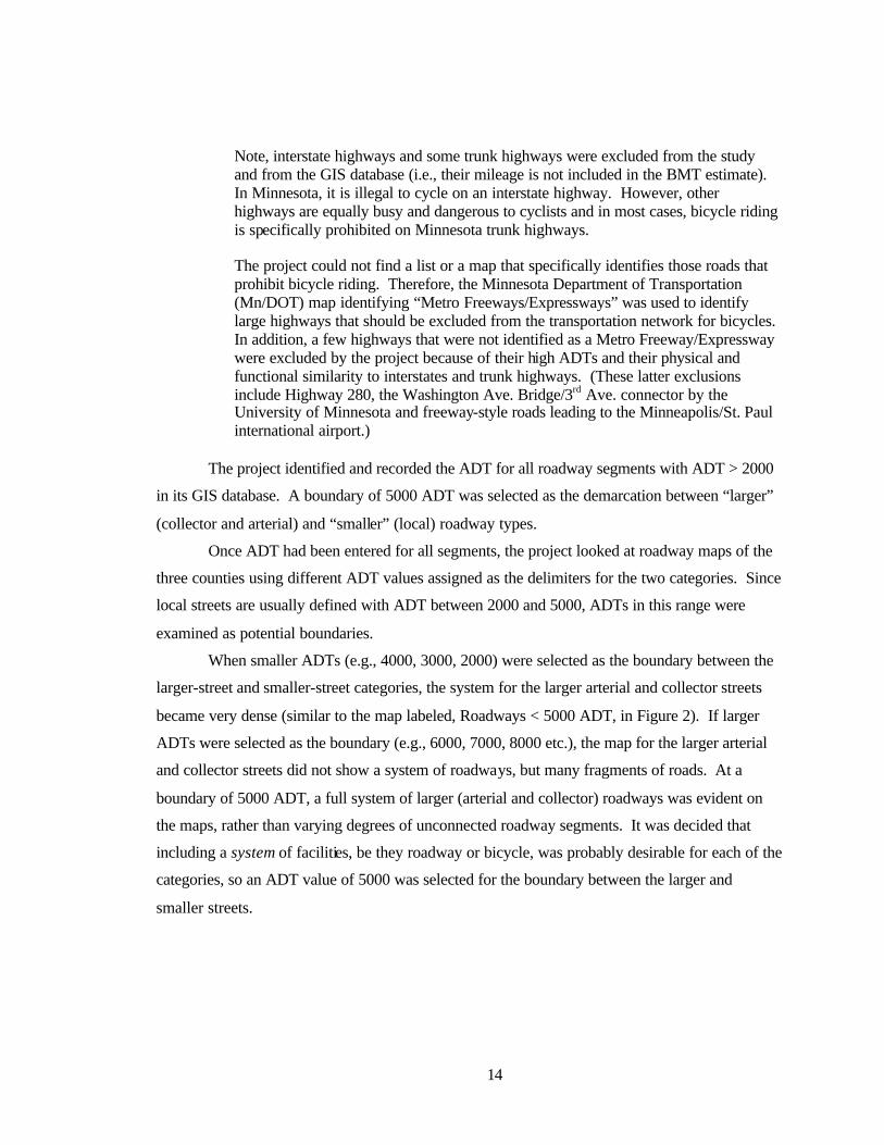
Note, interstate highways and some trunk highways were excluded from the study and from the GIS database (i.e., their mileage is not included in the BMT estimate). In Minnesota, it is illegal to cycle on an interstate highway. However, other highways are equally busy and dangerous to cyclists and in most cases, bicycle riding is specifically prohibited on Minnesota trunk highways. The project could not find a list or a map that specifically identifies those roads that prohibit bicycle riding. Therefore, the Minnesota Department of Transportation (Mn/DOT) map identifying “Metro Freeways/Expressways” was used to identify large highways that should be excluded from the transportation network for bicycles. In addition, a few highways that were not identified as a Metro Freeway/Expressway were excluded by the project because of their high ADTs and their physical and functional similarity to interstates and trunk highways. (These latter exclusions include Highway 280, the Washington Ave. Bridge/3rd Ave. connector by the University of Minnesota and freeway-style roads leading to the Minneapolis/St. Paul international airport.)

The project identified and recorded the ADT for all roadway segments with ADT > 2000

in its GIS database. A boundary of 5000 ADT was selected as the demarcation between “larger”

(collector and arterial) and “smaller” (local) roadway types.

Once ADT had been entered for all segments, the project looked at roadway maps of the

three counties using different ADT values assigned as the delimiters for the two categories. Since

local streets are usually defined with ADT between 2000 and 5000, ADTs in this range were

examined as potential boundaries.

When smaller ADTs (e.g., 4000, 3000, 2000) were selected as the boundary between the

larger-street and smaller-street categories, the system for the larger arterial and collector streets

became very dense (similar to the map labeled, Roadways < 5000 ADT, in Figure 2). If larger

ADTs were selected as the boundary (e.g., 6000, 7000, 8000 etc.), the map for the larger arterial

and collector streets did not show a system of roadways, but many fragments of roads. At a

boundary of 5000 ADT, a full system of larger (arterial and collector) roadways was evident on

the maps, rather than varying degrees of unconnected roadway segments. It was decided that

including a system of facilities, be they roadway or bicycle, was probably desirable for each of the

categories, so an ADT value of 5000 was selected for the boundary between the larger and

smaller streets.

15

Discussion

Regarding the categorization of bicycle facilities, design standards have been set for

building bicycle facilities23 and a functional classification of bicycle facilities has been offered.24

Regarding the former, these categorizations strictly address how facilities should be designed and

do not speak to how facilities might be used by bicyclists as part of a functional transportation

system. The latter addresses functional bicycle facility use, but has not been formally adopted.

Therefore, with the sampling requirements set forth by the GUTVC in mind, study

personnel reached the classification described in the preceding section by first considering the

fundamental milieu cyclists find themselves in. Cyclists find themselves on two basic types of

facilities. They travel a) on facilities that are visually and spatially designed for them and b) on

streets and roadways with no visual or spatial definition for bicycle use.

Within these two basic categorizations, there are further fundamental classifications of a

cycling environment. There are two basic sub-classifications of bicycle facilities with spaces

defined for cyclists: on-road and off-road bicycle facilities. And, there are two basic sub-

classifications of streets and roadways with no space described for bicycles: “larger, busier”

streets with a higher traffic volume (ADT) and “smaller, quieter” streets with a lower traffic

volume (ADT). Thus, four categories were established which describe fundamental

environments (and differences in those environments) for cyclists:

1. Off-road bicycle facilities,

2. On-road bicycle facilities,

3. Roadways with no cycling facilities and ADT <5000 (smaller, quieter streets), and

4. Roadways with no cycling facilities and ADT ≥ 5000 (larger, busier streets).

Aside from this typological analysis of fundamental cycling environments, previous

explorations in 1996 by the Sustainable Transportation Initiatives Unit at the Minnesota

Department of Transportation (Mn/DOT) 25 indicated that some assumptions regarding cycling on

urban streets might not be true. The assumption sometimes made in bicycle planning and research

circles which the Mn/DOT inquiry seems to question holds that cyclists like to stay away from

busy, high volume streets, preferring quieter local streets. The four categories developed for this

project might further illuminate the Mn/DOT findings, which are reported as follows.

The Mn/DOT study did not use a random sample, but selected intersections (and the

streets leading to them) in and around Minneapolis and St. Paul to investigate. (Note the

16

Mn/DOT study defines on-road bicycle facilit ies as “bike lanes” and off-road bicycle facilities as

“bike paths.”)

Manual counts were taken on weekdays for a total of six hours at each site. The 1996

Mn/DOT study reports:

According to bicyclist volume usage graphs:

• High traffic volume (especially greater than 10,000 average daily traffic,) urban streets during weekdays had nearly as much bicyclist volume per mile as multi-use recreational paths.

• Combining bicyclist volume of bike lanes, bike paths and high traffic volume, urban streets create more than 75% of bicyclist volume per mile studied. All other (ten) street categories combined, create less than 25% of bicyclist volume per mile studied.

• Bicycle lanes, on average, received more than twice the bicyclist volume as multi-use (…) bicycle paths.

• Bicycle lanes received more than 5 times the transportation bicyclist volume as multi-use paths on separate travel corridors from streets

• Bicycle lanes received nearly half of all ”on-street” bicyclist volume per mile studied. When bicycle lanes are combined with high traffic volume, urban street, this “on street” bicyclist volume jumps up to slightly less than 75%.

• On average, streets studied had more than 60% of bicyclists riding on the street itself as opposed to riding on sidewalks. This average appeared to remain, even when there was an adjacent recreational path.

This study seems to suggest that adjacent recreational paths do not accommodate most of the (…) bicyclists in the street corridor. It also appears from this study [that] the best way to encourage bicycle use is to provide bicycle lanes on higher traffic volume, urban streets.26

Though not conclusive, the data from this small study suggests a different reality of

bicycle use from current assumptions. The study suggests that bicycle use might be more

prevalent on larger and busier streets than it is on off-road facilities and perhaps, on local streets.

On-street allocation of bicycle space (bike lanes) appears to increase bicycle use even more on

the larger streets.

Though the Mn/DOT study did not directly address local streets, it shows a category of

streets labeled “2000-10000 ADT with a poor bicycle comfort rating formula” as the least used

of their study’s types (6-10% usage). Conversations with Mn/DOT personnel involved in the

study confirmed that they considered these the traditional “local streets,” and that contrary to the

assumption of many, -- that cyclists prefer local streets to collectors and arterials, -- the study

appeared to show the opposite.

17

The four types of bicycle facilities defined by the BMT project categorize bicycle use in a

fundamental, logical, and typological manner. The definition of bicycle facilities in this way has

a number of benefits. A primary benefit is that the categorization is a simple one and

understandable. The categorization allows the collected data to address fundamental issues of

bicycle use. The categorization provides an equal number of counts on bicycle facilities and

regular roadways. It allows the categories to be combined in different ways to raise and address

questions other than BMT, yet address them in a straightforward manner (e.g., bicycle facilities

vs. roadways with no facilities, or off-road bicycle use vs. any on-road bicycle use.

18

Sample Based Estimation of Bicycle Miles of TravelUniversity of Minnesota

Department of Civil Engineering

S1Urban

SUUniversity of Minnesota

S2Suburban

S3Exurban/Rural

Geographic Subareas Showing Roadwaysin the 3-County Twin Cities Metro Area

Figure 3. Geographic Subareas

19

3.4. Geographic Subareas

This section is divided into two subsections. The first describes the geographic subareas

established by the project. The second subsection discusses how the subareas were established

and provides commentary on the defined subareas.

Definition

In addition to recommending the definition of transportation facility types, the GUTVC

recommended that geographic subareas be established within the study area. The project

established the following four subareas with the following characteristics (see Figures 3 and 5):

• Urban Highest density of roadways Grid street system High connectivity of existing streets and roadways Overall, medium to sparse density of bicycle facilities

• Suburban Medium density of roadways Non-grid, street patterns; many culs-de-sac and eyebrow street types Lower connectivity of existing streets and roadways, many dead-ends Dense bicycle system

• Rural Low density of roadways Grid roadways follow section lines, small towns High connectivity of existing streets and roadways Very sparse bicycle system

• University of Minnesota (The area is described by a radius approximately 1 mile from the University of Minnesota’s East Bank and West Bank campuses in Minneapolis)

Has characteristics of the urban subarea Medium density of bicycle facilities Observations, together with previous counts and surveys show a high bicycle mode share around this U of M campus and therefore, a separately identifiable homogenous zone of bicycle use.17

20

Discussion

Project personnel studied the roadway and bicycle network maps produced in the previous

tasks and used their collective knowledge of bicycle use in the area to develop guidelines for the

division of the area into subareas of homogenous bicycle use.

• First, it was assumed that there would be a difference between bicycle use in rural areas

as compared to urbanized areas.

• Second, it was assumed that there would be a difference in bicycle use in the urban core

vs. the suburbs.

• And, finally, previous counts (specifically in October 1994) and general observation

around the Minneapolis Campus of the University of Minnesota showed extremely dense

bicycle traffic compared to other urbanized areas. (The 1994 counts showed that 10% -

21% of all vehicles on the road in the U of M area were bicycles.)

In addition, once all of the bicycle facilities and the ADTs for all of the roadways were

entered into the GIS database, patterns of transportation system density and roadway configurations

could be seen on GIS-generated maps, as seen in Figure 4, Figure 5 and Figure 6. (Note the patterns

for the roadway system in Figure 5 are more readily apparent on maps larger than the page size of this

report.) It was noted that the bicycle network was the densest in a ring encircling the inner core of the

Twin Cities area (Figure 4). The bicycle networks in the inner core and in the rural area, outside of

the dense ring, were sparse compared to the bicycle networks in the suburban ring. The roadway

network, however, was most dense in the inner core and less dense in the suburban ring (Figure 5).

And, as expected, the sparsest system of roads was in the rural area.

Thus, concentric rings of roadway and bikeway density were apparent on both the bicycle

facility maps and on the roadway maps. Within the urbanized area, there was a sort of inverse

relationship between the two different target-like configurations where roadway and bicycle network

densities were concerned. The inner core had the densest roadways compared to the suburban ring.

However, the bicycle facilities in the inner core were significantly less dense than those in the

suburban ring.

21

Sample Based Estimation of Bicycle Miles of TravelUniversity of Minnesota

Department of Civil Engineering

Patterns & Densities

Rural/Exurban Subarea

Suburban Subarea

Urban Subarea

On-Road & Off-Road Bicycle Facilities

Figure 4. Patterns and Densities – On-Road & Off-Road Bicycle Facilities

22

Sample Based Estimation of Bicycle Miles of TravelUniversity of MinnesotaDepartment of Civil Engineering

Patterns & Densities

Rural/Exurban Subarea

Suburban Subarea

Urban Subarea

Roadways

Figure 5. Patterns and Densities - Roadways

23

There was also a relationship between roadway and bikeway density and system connectivity. The

roadway maps clearly showed distinctions in roadway patterns that roughly followed the distinctions

in roadway and bicycle system density (Figure 6). The street pattern of the inner core consistently

showed a grid system of straight streets, with high connectivity in general and high connectivity of

different street types (e.g., in addition to arterial/collector intersections, there are many intersections

of arterial streets and local streets). The street patterns in the suburban ring consisted almost entirely

of curvilinear roads, culs-de-sac and eyebrow street types. The suburban cul-de-sac and eyebrow

street types are the local streets of the implementation of the functional hierarchy of streets in the

suburbs. The strict implementation of the functional hierarchy of streets (arterial, collector and local)

results in a system of more controlled access and less overall connectivity.

24

Sample Based Estimation of Bicycle Miles of TravelUniversity of Minnesota

Department of Civil Engineering

Pattern & Density Samples

Highest density of roadwaysGrid street patternHigh connectivity in generalHigh connectivity of street types

Medium density of roadwaysNon-grid street pattern

Many culs-de-sac & eyebrow street typesLower connectivy, many dead ends

Urban Subarea (S1)

Suburban Subarea (S2)

Urban & Suburban Roadways

Figure 6. Pattern and Density Samples – Urban and Suburban Roadways

25

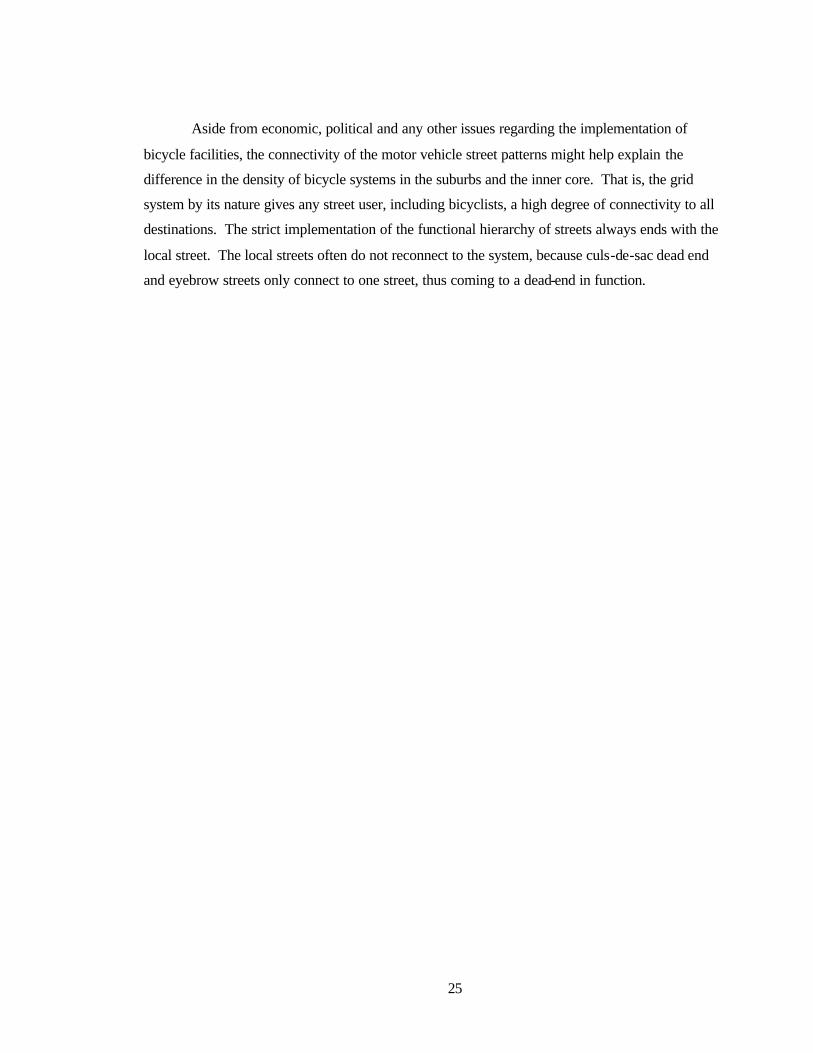
Aside from economic, political and any other issues regarding the implementation of

bicycle facilities, the connectivity of the motor vehicle street patterns might help explain the

difference in the density of bicycle systems in the suburbs and the inner core. That is, the grid

system by its nature gives any street user, including bicyclists, a high degree of connectivity to all

destinations. The strict implementation of the functional hierarchy of streets always ends with the

local street. The local streets often do not reconnect to the system, because culs-de-sac dead end

and eyebrow streets only connect to one street, thus coming to a dead-end in function.

26

Sample Based Estimation of Bicycle Miles of TravelUniversity of Minnesota

Department of Civil Engineering

Suburban Connectivity

Roadway > 5000 ADTRoadway < 5000 ADTOn-road Bicycle FacilityOff-road Bicycle Facility (not next to road)Off-road Bicycle Facility (next to road)

Bicycle & Roadway Systems

Figure 7. Suburban Connectivity – Bicycle and Roadway Systems

27

Roadway connectivity (as allowed by the different types of street patterns) could be

indicative of the need for bicycle facilities. With low connectivity, bicycle facilities are more

necessary so that cyclists can connect to their destinations conveniently and in a time efficient

manner. The suburban ring in the three counties clearly shows the existence of more bicycle facilities

and bicycle facilities designed to enhance connectivity in conjunction with the roadway system.

Figure 7, taken from the GIS maps of a Minneapolis suburb, has many examples of this.

Analysis of the GIS-generated maps showing metro area roadway and bicycle systems

confirmed the initial analysis of the types of subareas that project personnel formulated. Whether

connectivity and density play a role or not, there were clearly four different subareas visible on the

GIS maps that indicated there could be homogeneity of bicycle use. The four subareas represent

fundamental differences in transportation system design, and roadway and bicycle system density.

Like the four bicycle facility types, the definitions of the four different subareas are straightforward

and easy to understand.

28

3.5. Study Characteristics

The table below shows the number of segments of each facility type in each subarea and

county. Additional characteristics of the study area include a relatively flat terrain with slopes

occasionally exceeding 10%. Only one of the randomly selected count sites was not on flat

terrain. This site was located on a segment of a regional park trail. Neighboring segments of the

selected count sites were also on flat terrain. Thus, topography probably played no role in use of

either roadways or bicycle facilities by cyclists.

Counts were taken from mid-May through the first week in July and between the end of

August and the middle of October. The weather during the count period was seasonably pleasant.

The autumn time period, from the end of August to the middle of October was unseasonably

warm and sunny. Thus, a variety of warm season counts were taken during the study.

Table 1. Numbers of Segments by Facility Type, Subarea and County

Bicycle Facilities Roadways with no Bicycle Facilities

On-road Off-Road <5000 ADT ≥5000 ADTa TOTAL

University subarea (SU) Dakotab

Hennepin Ramseyb

SU Total

None

48 None

48

None

28 None

28

None

178 None 178

None

76 None

76

None

330 None 330

Urban subarea (S1) Dakota

Hennepin Ramsey

S1 Total

2

280 216

498

24

469 249

742

1426

17869 8591

27886

223

3767 2102

6092

1675

22385 11158

35218 Suburban subarea (S2)

Dakota Hennepin

Ramsey S2 Total

388 529 610

1527

1081 3257 1224

5562

9908

17947 7261

35116

740

1821 660

3221

12117 23554 9755

45426 Rural/exurban subarea (S3)

Dakota Hennepin Ramseyb

S3 Total

149 37

None 186

113 57

None 170

2791 2497 None

5288

231 211

None 442

3284 2802 None

6086

Dakota Hennepin

Ramsey TOTAL

539 894 826

2259

1218 3811 1473

6502

14125 38491 15852

68468

1194 5875 2762

9831

17076 49071 20913

87060

a Does not include interstates and trunk highways. See section 3.3. b County does not contain this subarea or facility type.

29

3.6. Data Collection

3.6.1. Overview and Checklist

For those who might wish to conduct a similar BMT project, the contents of the

introduction to this chapter are listed in checklist format. Details and commentary are found in

the subsections that follow.

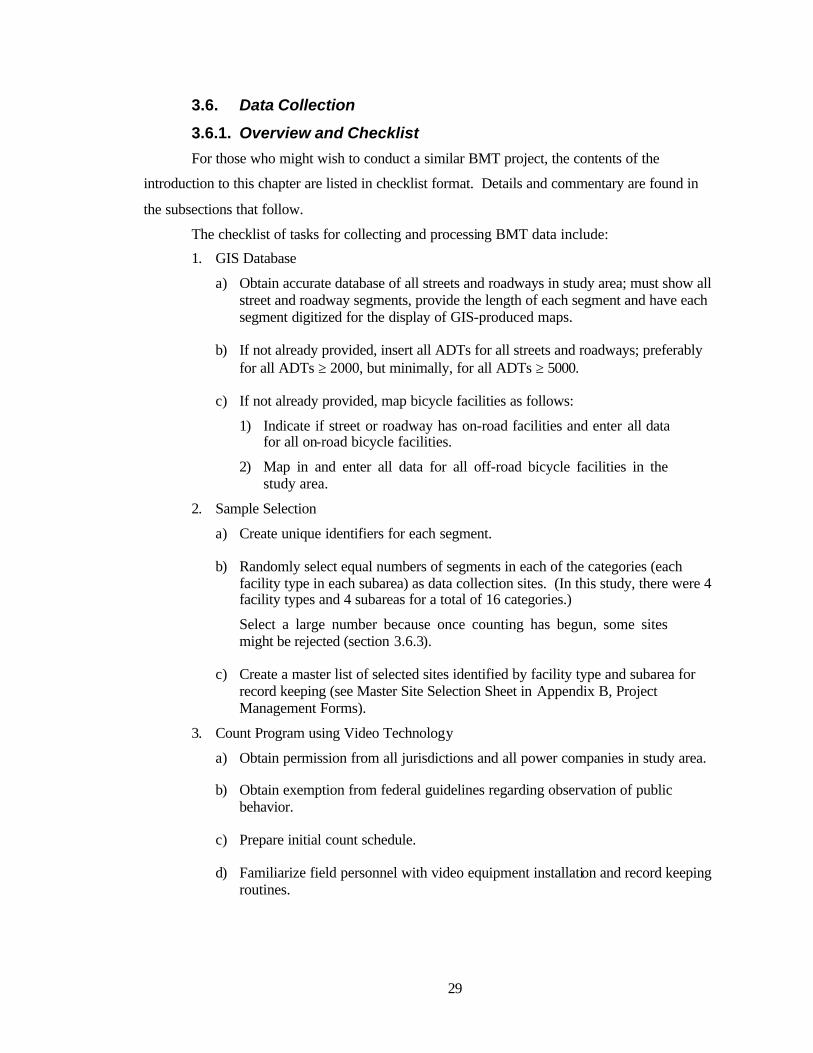
The checklist of tasks for collecting and processing BMT data include:

1. GIS Database

a) Obtain accurate database of all streets and roadways in study area; must show all street and roadway segments, provide the length of each segment and have each segment digitized for the display of GIS-produced maps.

b) If not already provided, insert all ADTs for all streets and roadways; preferably for all ADTs ≥ 2000, but minimally, for all ADTs ≥ 5000.

c) If not already provided, map bicycle facilities as follows:

1) Indicate if street or roadway has on-road facilities and enter all data for all on-road bicycle facilities.

2) Map in and enter all data for all off-road bicycle facilities in the study area.

2. Sample Selection

a) Create unique identifiers for each segment.

b) Randomly select equal numbers of segments in each of the categories (each facility type in each subarea) as data collection sites. (In this study, there were 4 facility types and 4 subareas for a total of 16 categories.)

Select a large number because once counting has begun, some sites might be rejected (section 3.6.3).

c) Create a master list of selected sites identified by facility type and subarea for record keeping (see Master Site Selection Sheet in Appendix B, Project Management Forms).

3. Count Program using Video Technology

a) Obtain permission from all jurisdictions and all power companies in study area.

b) Obtain exemption from federal guidelines regarding observation of public behavior.

c) Prepare initial count schedule.

d) Familiarize field personnel with video equipment installation and record keeping routines.

30

4. Scheduling and Management

a) Prepare site lists and site maps, installation sheets and count sheets (see Appendix B, Project Management Forms.)

b) Monitor installations and supervise installation scheduling

5. Bicycle Counting (for BMT estimation)

a) Count each individual cyclist as he/she passes on the selected segment.

b) Count only cyclists on the selected corridor segment (i.e., not on adjacent segments or in neighboring intersections).

c) Count all cyclists in the corridor, whether on the bicycle facility, in the street or on sidewalks.

d) For convenience and additional information, record at 15-minute intervals and record weather.

e) Count tandem cyclists as one count (vehicle miles of travel are measured in bicycle miles of travel, not person miles of travel).

3.6.2. GIS Database

Any project measuring BMT or other volumes of bicycle traffic on a large scale requires

a database to minimally provide basic data such as total length of the system. A Geographic

Information System (GIS) product is recommended to manage the data and to provide maps of

the study area and facility types. GIS products correlate data with maps. That is, a database

accompanies each roadway map and each defined roadway segment in the map has a data entry.

Serious errors could occur without the GIS ability to produce maps from the data, particularly

when the study area and therefore, the data are of any size.

The project used the Arc View GIS product from ESRI Corporation. The base data for

the streets and roadways in the Twin Cities area was the street centerline database that Mn/DOT

and the Metropolitan Council jointly developed with an outside vendor in 1996-97. The street

centerline database was developed to provide common base data for researchers, planners and

mapmakers of roadways in the Twin Cities area and to provide base data that was more accurate

than that which was used in the past. This project was one of the first users of the new database.

The project added ADT and bicycle information to the base data for each roadway in

three metropolitan area counties: Hennepin, Ramsey and Dakota. Seven County Street Series

Traffic Volume Maps (1996) produced by Mn/DOT and USDOT were examined to identify all

31

roadways in the three county area with an ADT >2000. If ADT was ≥ 2000, the segment data

was amended to include the segment’s ADT. For segments <2000ADT, the ADT was set to zero.

The ADT was given a value of 1 for anomalies (e.g., usually a small segment indicating an

arterial crossing in the original base data, see Figure 8). (See section 3.3 for a discussion on why

ADT=5000 was selected as the boundary between the larger street category and the smaller one.)

The next task in the development of the project database was the entering of data for on-

road bicycle facilities and the mapping and entering of data for off-road facilities. This task

sometimes required contacting appropriate personnel in each jurisdiction. It was often necessary

to resolve differences between the maps produced by the different jurisdictions (e.g., county maps

vs. community maps). Also, since each jurisdiction categorized their facilities in the manner they

saw fit, it was sometimes necessary to determine how their classification of bicycle facilities fit

within the classification system of this study or with classifications used by other communities.

Finally, since bicycle maps are not produced every year, it was necessary to determine if facilities

marked as scheduled for construction were indeed built on schedule.

The project used Digital Orthographic Quadrangle aerial photographs (DOQs)27 as a

tracing base for mapping the off-road bicycle facilities. At the time of the study, it was not

practical or possible to digitize the off-road facilities (i.e., manually transfer the bicycle facilities

from accurately measured maps, which are precisely registered with the maps in the database).

One reason digitization was not possible was that exact locations and lengths of off-road bicycle

facilities are not as precisely surveyed or mapped as are motor vehicle roadways. Off-road

bicycle facilities, for example, are not found on USGS maps, which have the necessary precision

for digitization. It was, therefore, not possible to digitize off-road bicycle facilities for the BMT

project from available maps. And thus, the off-road bicycle facilities were traced from DOQs

onto the Metropolitan Council’s Street Centerline Map as a base.

32

Sample Based Estimation of Bicycle Miles of TravelUniversity of Minnesota

Department of Civil Engineering

Roadway AnomaliesOmitted from Study

UNIVERSITY AVE WUNIVERSITY AVE W

University Avenue in St. Paul is a large arterial.

Intersections like the highlighted ones seen here,were omitted from the study. If they had beenincluded and selected for a count, it would havebeen unclear which segment was to be counted(University Avenue or a cross street).

Figure 8. Roadway Anomalies not included in the Study

33

Next, the project used the GIS mapmaking flexibility to produce maps to analyze how the

subareas for the study were to be defined and where the boundaries were to be set. Section 3.4

discusses the analysis used to define the four subareas that are used in this study. Project

resources did not permit individually assigning each roadway segment and each bicycle segment

in the database to a specific subarea. The project therefore looked at subarea demarcation

according to community boundary (the subarea designation could be marked in the database as a

group of roadways segments located within a specific community because community name was

a field in each segment’s data record). Visual examination of the characteristics of the roadway

and bicycle systems in the four subareas showed a close correlation between community

boundaries and the subarea characteristics (also described in 3.4).

As a final note, the street centerline database is organized by county. ADTs, and on-road

and off-road bicycle data were added as new fields in the database accompanying the street

centerline map. In the case of off-road facilities, new records were added to the street centerline

base data and new segments were added to the map, making one large database per county that

shows all roadway and bicycle information in the county. Since GIS product capabilities allow

users to make subsets of this information or to merge or join databases, the user has significant

flexibility in subdividing and analyzing the data.

34

Sample Based Estimation of Bicycle Miles of TravelUniversity of Minnesota

Department of Civil Engineering

Counted Sites

Figure 9. Counted Sites

35

3.6.3. Sample Selection

As discussed in section 3.2, the Guide to Urban Traffic Volume Counting recommends

that each facility segment be classified with a subarea and a facility type. The BMT project

defined four facility types and four subareas. Therefore, there were a total of 16 unique

classifications in the BMT study.

Each classification must have an equal number of counts and the count sites must be

randomly selected. Therefore, each segment in the database must be uniquely identified. Since

the street centerline database was organized according to county, the intra-county identifier

supplied with the original data was not unique on an inter-county basis (i.e., county-id #1, #2, …

etc. was assigned in each of the three counties.) Inter-county (unique) identifiers assigned in the

street centerline base data were not adequate because of their inconvenience to project

researchers. That is, the sequential nature of the assignment of the inter-county identifier did not

allow off-road bicycle facilities to be added and numbered in a logical, easily understood fashion.

The inter-county identifiers proceeded sequentially through all nine counties of the Twin Cities

metro area. The addition of identifiers for off-road bicycle facilities would necessarily have had

to begin at the end of the last number in the last county. While this would have worked, it would

have become quite confusing to understand segment identifiers for purposes of the study.)

Thus, the project assigned each of the 16 classifications its own series of identifiers,

beginning with 1 in Dakota County and ending in Ramsey County. Appendix B-3 shows the

assignment of bicycle identifiers for purposes of this study. Note, since numbers are duplicated

across the 16 classifications, every bicycle identifier is qualified by its subarea and bicycle

facility type (i.e., subarea, facility type, ID).

If more studies of this kind are conducted and as new segments are added to the database,

it may be necessary to reassign new bicycle identifiers (and erase old ones) for purposes of

selecting a random sample and managing the count project. This would be done to simply make

it easier for researchers to understand which range of identifiers belongs with which type of

facility/subarea. Doing this would not affect any record keeping since all data and geocoding

information is carried with the segment’s record in the database. The renumbering of identifiers

in the future would not affect any previous or subsequent bicycle studies using the database first

established by the BMT project.

36

After identifiers were assigned in each of the sixteen classifications, the random number

generator provided with Microsoft Excel 97 was used to randomly select the count sites. Figure 9

shows all of the sites that were counted in the study; i.e., 10 sites in each of the 16 classifications,

or 160 sites.

Technically speaking, the days on which bicycle count data were recorded should also

have been randomly selected. However, if this had been done, the cost of travel to sites that were

also randomly selected according to day of the week would have been prohibitive since travel

time to the count sites was the most consumptive of project time during the data collection phase.

For example, three count sites for a particular day; if also randomly selected by day of week

could require over 150 miles of travel time per day. Even when sites were “clustered,” as

described next, 60 miles per day was the average travel distance. This average included 25% of

the sites, which were located around the University of Minnesota, the “home base” of the project.

Mn/DOT and project personnel decided that the “clustering” of sites was necessary. In

other words, sites that were near each other or “on-the-way” to each other were counted on the

same day. However, two or more sites where the same cyclist could potentially be counted

within a short period of time were not selected for counting on the same day or, even on

sequential days. Though not calculated, it appears that this method of counting was fairly random

because distances between the randomly selected sites were usually significant. (For example,

three sites in south Minneapolis, while appearing fairly close together on an 8½ x 11 map Figure

9, were in reality located in three different neighborhoods, all of which were not located next to

each other.)

3.6.4. Count Program

The project used traffic video recording technology from ATD Northwest in Redmond,

WA to videotape the count sites. Research assistants then counted cyclists from the videotape.

Two people were required for equipment installation because the box housing the VCR and

marine battery was too heavy and bulky to install by one person. Also, it was more efficient to

have a driver and a navigator whose job it was to locate sites and direct the driver to them.

Videotaping cyclists is more time- and cost-effective than using human counters on-site

for a number of reasons. First, human counters should usually not be scheduled for more than 4-6

hours per day because of the nature of the work. Since the manual counting of bicyclists for even

this amount of time is fairly boring, especially if the human counter works on a regular basis,

37

manual bicycle counts are usually less reliable for collecting count data than an automatic means

of collecting the data. Using human counters to collect data also requires significantly more

scheduling management; on-site, employee supervision; and travel time to replace personnel

during the count day. These requirements significantly increase data collection costs.

Previous tests of other bicycle count technologies (e.g., tube counters and laser counters)

showed both were not satisfactory methods for counting bicyclists. Tube counters tested by the

City of Minneapolis and Mn/DOT’s Sustainable Transportation Initiatives Unit showed that they

are probably not a reliable method of counting cyclists for a number of reasons. For example, a

tube counter placed on an off-road, multi-use facility in Minneapolis was carefully wound up and

placed off of the bicycle facility by a facility user. (Since the counter was carefully wound up

and not vandalized, it was presumed that perhaps the tube counter tripped roller blade users, or

even interfered with cyclists.) In addition, tube counters do not effectively count cyclists on city

streets, where despite even the presence of a striped facility, bicyclists can be found in any place

within the street corridor, including the sidewalk. (Note: as discussed in section 3.6.5, all cyclists

within the right-of-way corridor space were counted as users despite the location or kind of

bicycle facility found in the corridor) The use of laser counters could be very problematic in

urban areas and in non-urban areas, the Minnesota Department of Natural Resources found that

deer and hikers were counted by a laser counter.

The collection and counting of bicycle data is the most time-efficient when traffic video

recording technology is used. The ATD Northwest recording technology is pole -mounted and is

usually installed in 5-10 minutes and removed in less than 5 minutes. The technology permits the

recording of data at selected time intervals. This, therefore, uses less videotape and requires less

time to count bicyclists from the tape. The project found that with a setting of one frame per 5

seconds, one two-hour tape could record more than 24 hours of on-site counts. The project

actually counted from 5 AM to 10:30 PM, or 17.5 hours each day; i.e., the longest time of

daylight and twilight in a Minnesota summer. Preliminary tests by Mn/DOT and project

personnel showed almost no cycling after dark. In addition, unless the camera was positioned

near a streetlight and cyclists traveled in the light thrown by the streetlight, nighttime cyclists

could not be seen on the videotape. (Since counts were taken into the shorter days of October and

exact time periods for all counts are required for the BMT estimate, the project used 12 hours of

count time, from 7 AM to 7 PM to formulate the BMT estimate.)

38

Bicyclists recorded for a 17.5 hour period on a video tape using 5 second timed intervals

could be counted in approximately 1½ - 6 hours by project research assistants, depending on the

number of automobiles, bicycles and pedestrians found in the corridor. The busier the corridor,

the more time it takes to accurately discern and count individual cyclists. Nevertheless, the count

time from videotape is significantly more time-efficient than stationing human counters on-site

for seventeen hours.

As noted in section 3.6.5, even though the nature of the corridor facility type (e.g., on-

street facilities) might have precluded cyclists from some areas of the corridor, (e.g., motor

vehicle traffic lanes or sidewalks), bicycles within any part of the corridor were counted. This

was done because the purpose of the study was to determine bicycle miles of travel and not the

nature of facility use.

Hidden and potential barriers to obtaining bicycle counts from videotape are permissions

required from:

1. Communities in which the selected sites are located, 2. Electrical power companies on whose poles the equipment is installed, and

3. Agencies authorized to apply federal guidelines regarding the observation of public

behavior.

Failure to obtain permission to videotape from any of the above can terminate a count

program or research using videotape.

To obtain permission from communities, the project issued a mailing containing:

1. A brief, one-page explanation of the project, 2. Photos and a description of the video recording technology,

3. A list of selected count sites showing address range and street name of the selected

sites within the community (an example site sheet is shown in Appendix B-5), and 4. A simple permission form for return to the project (Appendix B-1).

Communities had a variety of questions and concerns and sometimes altered the

permission form to suit their concerns and needs. Different communities placed responsibility for

bicycle facilities in different types of city offices including planning, parks and recreation, traffic

engineering, and law enforcement. Rather than call each community, the project found that the

most efficient way of steering the information and the permission form to the appropriate place

39

within any community government was to initially address the permission packet to Traffic

Operations. The project found that if this was done, the information quickly reached the

appropriate party.

In the Twin Cities area, the video recording technology usually needed to be installed on

power poles owned by the area’s electrical utility. Since electrical utilities own these poles,

permission is also needed from them to install equipment on their property.

One obstacle the project encountered, particularly in the case of power companies (and

somewhat with communities), was that the company had never received or processed a request

for mounting equipment on their poles for one day only. The closest type of request the Power

Company had experienced was from businesses using microwave communications technology.

These companies rented power poles for years at a time. For whatever the reason, because a

request to videotape the roadway corridor is an entirely new one, personnel from any bicycle

count project and representatives from a power company must initially devote considerable time

to find who is responsible for granting permission and how it will be granted. However, once

done the first time, permission to obtain future counts should be accomplished fairly quickly.

Rather than issue a lease for each pole, as is usually the case, the power company in the

Twin Cities area decided to amend (shorten) their master lease agreement to include a general

description of where and how the equipment was to be installed on any pole (see Appendix C).

Regarding the latter, was the Power Company’s concern regarding the installation of video

recording equipment on painted aluminum poles and on fiberglass poles. Some communities also

shared these concerns regarding the use of light poles that they owned. The Power Company that

was involved in the BMT project decided that the use of painted poles (i.e., aluminum) was

permitted if padding was placed around the equipment. Project personnel found this to be more

than adequate for protecting the pole. Future projects should investigate whether the equipment

is too heavy for fiberglass poles. This was not pursued by the BMT project because count delays

due to all of the needs for obtaining permission to videotape had significantly increased. In

addition, all of the selected sites proved to have poles made of other materials.

The issuance of a master lease agreement from the Power Company initiated another

involved process at the University of Minnesota to process such a request. It should be noted by

any other projects measuring bicycle use in this way, that the Power Company required liability

insurance in the amount of several million dollars. This was not a problem for the University of

Minnesota because it maintains insurance of this nature for all sorts of different uses. It should

40

also be noted that for its part, the University found it necessary to negotiate a few details of the

agreement with the power company and that ultimately the master lease agreement required five

signatures at the University, including representatives from University leasing and asset

management offices, department heads, deans, and vice presidents.

Some communities and the power company initially requested that project personnel and

community/power company personnel visit all of the selected counts sites, select a pole on which

the video equipment was to be installed and note the location on the pole where the equipment

would be installed. Some communities and the Power Company requested payment for this

process (a significant amount compared to project resources). In the case of communities, poles

had in the past been individually selected for the installation of loudspeakers at picnics and

gatherings (less than a handful of sites). In the case of the Power Company, pole rental sites were

to be used for years by a commercial concern, so the cost could be absorbed. Since this process

was cost prohibitive to the project, the difference in the nature of use, the amount of pole rental

time and the nature of the equipment were discussed. Regarding the latter, it was pointed out that

the equipment had a self-contained power source; that once installed, it would not physically

interfere with other equipment on the utility pole and would not easily be noticed. The Power

Company and some communities agreed that the site inspection process was not necessary for

this type of project.

In some cases, communities did not respond to the project’s permission request or they

placed such time-consumptive requests on the project for equipment demonstrations or

explanation of the nature of the data collection process, that the project had to forego the

inclusion of the community in the count process. However, enough communities comprising a

representative sample of all of the subarea types did respond and so count sites in those

communities were included in the project sample.

The final issue that any video counting project must address is permission to observe

(videotape) public behavior. The observation of public behavior is regulated by federal policy as

stated in the Code of Federal Regulations, Title 45, Part 46 (45 CFR 46). This federal policy

requires permission from an appropriate regulating agency (e.g., the University of Minnesota’s

Institutional Review Board, IRB) to record public behavior for purposes of research.

The BMT project obtained an expedited review to videotape public behavior for purposes

of counting cyclists. The expedited review took significantly less time than full committee

review. Conditions that the project was requested to satisfy included assurance that individuals

41

could not be identified, storage of the tapes in controlled conditions, counting of the tapes by

selected personnel only and erasure of the tapes when the project concluded.

Appendix D, Protection of Human Subjects, contains a list of federal and University of

Minnesota websites where further information can be obtained on federal policy for the

protection of human subjects.

In summary, all of the agencies and jurisdictions requiring review and permission to use

traffic video technology for collecting the bicycle count data should be contacted prior to the

initiation of any research or bicycle count project of this type. When the BMT project initiated its

proposal and its work plan for the project, none of the requirements described above were known.

The additional needs for obtaining all of permissions described above placed significant stress on

project resources, specifically those designated for project management.

It should be noted, however, that once the processes for obtaining permission for this type

of effort are completed the first time, it should be considerably shorter and easier on subsequent

count projects. For subsequent efforts, a “permission infrastructure” would be in place and

appropriate personnel in various agencies, jurisdictions and companies would be identified and

knowledgeable of the purposes of similar projects and the processes required to gain permission

for collecting data.

3.6.5. Counting Guidelines

The BMT project adhered to the following when counting cyclists from the videotape.

• Only cyclists who rode on the selected segment were counted. Often, adjacent

segments and intersections could be seen on the videotape. Counts were not made of

cyclists who were on adjacent segments but did not enter the selected segment. In

these cases, the cyclist either crossed through the adjacent intersection on the cross

street, or turned off the corridor or parked prior to entering the selected segment.

• For BMT estimations, all cyclists within the selected corridor segment were counted,

despite the type of bicycle facility found in the corridor (on- or off-road) or existing

laws regarding bicycle use in the corridor (e.g., no cycling on sidewalks). The

purpose of a BMT calculation is to determine bicycle miles of travel and not the

nature of facility use. Therefore, sidewalk cyclists and cyclists traveling outside of

an on-road or off-road bicycle facility (e.g., in the roadway) were counted.

42

• Tandem cyclists were counted as one count (vehicle miles of travel are measured in

Bicycle Miles of Travel, not Person Miles of Travel).

• For convenience and additional information, counts and weather conditions were

recorded at 15-minute intervals.

3.6.6. Scheduling and Management

When this project was being conceived in its proposal phase, it was thought that a

schedule for a few weeks or more could be set and that field personnel could simply install the

video equipment according to a list of sites. This proved not to be the case. In fact, significant

time was necessary to manage and schedule equipment installation. On the BMT project, the

project manager performed this, though a field supervisor could be trained to do it.

The reasons for scheduling management are several; including clustering count sites for

more efficient travel to and from sites and the rejection of a count site by field personnel. In

addition, to use the equipment in the most time-efficient manner, the installation of the equipment

rotated in time on a day-to-day basis. These are discussed below.

Project personnel considered different scenarios or schedules of equipment installation

during the day. Since the video equipment had on/off times, which controlled the times of data

recording, the equipment could be installed at any time during the day and at different times on

each day. In other words, time of day, day of week and the continuous recording of data on one

day alone were not factors in collecting the data.

The project determined that the most time-efficient use of (rented) equipment was to

continually advance the schedule, rather than install the equipment at fixed times. In the worst

case when different types of fixed schedules are used, an entire day would have to elapse between

field installations of a particular camera. For example, if a camera were scheduled for an 8:00

installation throughout the project, it would be necessary to install the camera every other day.

The installation and travel times involved in the installation process would make it necessary to

wait an entire day for the camera to be installed again at 8:00 AM.

Continually advancing the schedule allowed for the most time-efficient use of the

equipment. With a continually advancing schedule, if camera #1 was installed at 8:00 AM

Monday and removed at 8:00 AM Tuesday, it would be installed at the next site at some time

later than 8:00 AM Tuesday, say 9:00 AM, because of the travel time involved from site to site.

43

So, a continually advancing schedule advances in time until the camera or cameras are brought

“home.” (For safety reasons, research assistants did not install equipment after dark.)

A continually advancing schedule, though most efficient in the use of equipment requires

considerable scheduling management, because equipment installation and travel time cannot be

accurately determined beforehand. Equipment problems, obscure site locations, traffic jams and

so forth contribute to later installations than could be predicted beforehand. Moreover, with four

cameras in the field and a study area that was more than 30 X 30 miles wide, it was sometimes

found that it was the most efficient to bring a camera “home” and install it first thing on the way

to the other sites. Or, it was found that it was more efficient to de-install two cameras and then

install both of them before taking down the third camera.

Scheduling equipment installation in this way required regular review of the status of the

camera installations (when and where they were set up, and when and where they were to go).

The project found that it was usually not possible to schedule for more than four days in advance

and this only when the installation routes and so forth were straightforward and fairly well

known. More complicated sequences of installations required more scheduling management. In

addition, scheduling of equipment installation in this way required regular and frequent

production of map sheets and site sheets (Appendix B-5).

It should also be noted that this kind of scheduling, while providing the most counts in

the least amount of time, requires field personnel than can and are willing to continually change

their schedules on a daily basis (including weekends). This was relatively easy for the BMT

project because undergraduate research assistants were used in the summer months. Summer

session classes and the beginning of fall quarter classes made it considerably more difficult for

any of three research assistants to be available (two at a time) at once. Therefore, it was also

necessary for project management to be available to install cameras in the field.

Accurate record keeping and organization are critical on projects like this. Appendix B,

Project Management Forms, provides all of the record keeping sheets used by the BMT project,

described as follows:

• The master key shows the range of identifiers for each of the sixteen facility

type/subarea categories.

• The explanatory label to be taped to the video equipment helped identify the

equipment to curious passers-by or neighbors. Local police are sometimes informed

by the jurisdiction responsible for the roadway or bicycle facility. However,

44

sometimes notification is not thorough. Such a label can save time and unnecessary

interruptions. Wording like that shown in Appendix B is recommended since

gathering bicycle count data is largely supported by the public.

• The master site selection sheet shows the order in which each site was randomly

selected. This sheet can be marked up and used as a quick reference for project

management regarding sites that have been counted or need to be counted. If the

record identifiers are put into a table format, the sheet is automatically created by the

random number generator.

Note, in addition to clustering installation sites, project management or field

personnel had the option of rejecting sites. The most common reasons for this

included: danger either to project personnel or to equipment in the field; no pole on

which the equipment could be installed; roadway or bicycle facility closed due to

construction; and improper identification of the facility in the database (a few times,

the original base data recorded information regarding the roadway incorrectly; e.g.,

driveways to businesses were designated as local streets or maps provided by

communities indicated the existence of a bicycle facility where none existed).

Therefore, because of cluster-type scheduling and the option for site rejection, the

master site selection sheet is critical for keeping and reviewing records regarding

what has, has not, or should be counted.

• Site sheets contain the information that equipment installers require in the field for

finding sites and recording information about the camera installation.

• Site maps give detailed instructions in map form on how to reach the site. Sometimes

more than one map is needed to pinpoint the location of the site and to direct field

personnel to the site from home base or from a previous site.

The project found that automatic map production facilities provided on the Internet

produced information that was too detailed and not formatted for quick understanding

in the field. In addition, sometimes the Internet did not produce maps with the most

direct or the quickest route. Production of maps by project management took about

the same amount of time as producing, amending and reviewing internet-produced

maps. GIS mapmaking capabilities using the project’s database allowed project

management to quickly produce maps for use in the field.

45

• Installation sheets are used to record data in the field and provide a record of where

and when counts were actually taken. Of particular importance is the numbering of

video cameras and recording the camera number used at each count site. This is

necessary to more efficiently track malfunctioning equipment which is usually

detected when the tape is viewed and counted (fast forward will often not catch

equipment malfunction or other installation problems).

• Count sheets are used to record bicycle counts taken from the videotape. Project

personnel used hand-held counters and counted for fifteen minutes (as determined by

the video tape time-stamp, easily seen on the screen). Research assistants found that

a 15-minute interval was the most convenient and accurate interval for recording the

12 hours of counts. After 15 minutes, the researcher recorded the count data and

made note of the weather, which is also easily seen on the tape. Thus, the project was

able to gather extra information regarding bicycle use than specified by the project

proposal without using any extra count time. Providing information regarding

recreation vs. transportation use and bicycle contra-flow counts takes more time

because of the need for closer review and decision-making on the part of the counter.

Note the project found that recording the site identifier, subarea and facility type on all

records, including tape labels, was necessary to efficiently keep project records.

The BMT project required more project management than originally planned. An

unanticipated and lengthy permission process, as well as unanticipated scheduling and installation

management needs contributed to a significant increase in management time over that which was

planned at the project’s inception. However, management requirements of future projects will

decrease because of the “permission infrastructure” put in place by the first counting effort. In

addition, if future projects have the luxury of using cameras purchased by a DOT or other local

jurisdictions or agencies (rather than rented by the project), as well as gathering counts for

extended periods of time (or included in regular work routines), scheduling and project

management requirements might also decrease.

Project management time on the BMT project reached unanticipated levels of time

requirements because the project was the first of its type and scale, exploring new grounds in this

type of data collection. Despite this, the gathering of bicycle count data is an effort worthy of

continuation. The number of cyclists counted shows that there are more individuals cycling than

one might perceive in a casual manner. Since cycling is proving to be a space- and time-efficient

46

mode of transportation, especially in urban areas, it is worthwhile to measure and understand it as

much as motor vehicle transportation is understood. Once the management needs for conducting

bicycle counts are better understood and included as regular parts of transportation data collection

and planning routines, the entire process of measuring bicycle use will become easier and more

efficient.

47

Chapter 4 COMPUTING ESTIMATES OF BMT

4.1. Estimating Average Daytime BMT

The data collection and processing phase of this study produced a total of 160 12-hour

bicycle volume counts, ten in each combination of the four subareas and four facility types.

Appendix E of this report lists these counts along with other characteristics of the count sites. In

essence this constitutes a stratified random sample of bicycle volumes, where each combination

of subarea and facility type constitutes one of the sampling strata. To estimate total BMT from a

simple (not stratified) random sample of traffic counts, the GUTVC recommends using a ratio

estimator of the form

Xx

xvBMT n

kk

n

kkk

=

∑

∑

=

=

1

1 (4.1)

where

vk = counted volume on sample site k,

xk = length of sample site k,

X = total miles of roadway in the area of interest.

The ratio estimator requires information beyond what is included in the sample (in this case the

total roadway mileage) but when the numerator and denominator measurements are correlated,

the ratio estimator will usually be more precise than simply multiplying the average BMT

computed in the sample by the number of roadway links in the population28. When the sample

size n is larger than about 30, the standard error of the ratio estimator can also be estimated and

inferences concerning the BMT can be based on standard normal distribution theory.

Table 2 - Table 4 display the total mileage in the study area, sample BMT and sample

mileage, in each case broken down by subarea and facility type. Table 5 then gives the ratio

estimate of BMT for each subarea and facility combination. Because only 10 counts are available

for each stratum, the large sample theory should not be applied to these individual estimates.

48

Table 2. Total BMT on Sampled Links, in each Sample Stratum

Facility Type

Subarea

Off-Road Bicycle Facilities

On-Road Bicycle Facilities

< 5000 ADT

Roadways

> 5000 ADT

Roadways

S1

683.97

106.98

25.23

163.63

S2

112.68

12.53

12.32

32.10

S3

742.43

27.93

7.10

52.38

SU

414.32

393.26

143.94

256.84

Table 3. Total Mileage of Sampled Links in each Sample Stratum

Facility Type

Subarea

Off-Road Bicycle Facilities

On-Road Bicycle Facilities

< 5000 ADT

Roadways

> 5000 ADT

Roadways

S1

2.05

0.82

0.80

0.92

S2

1.96

0.77

0.91

1.41

S3

5.43

3.50

2.36

3.41

SU

1.01

0.69

0.94

0.71

49

Table 4. Total Mileage in Study Area in each Sample Stratum

Facility Type

Subarea

Off-Road Bicycle Facilities

On-Road Bicycle Facilities

< 5000 ADT

Roadways

> 5000 ADT

Roadways

S1

121.03

55.39

2472.24

580.93

S2

713.08

175.77

3488.37

507.57

S3

43.15

83.91

1369.83

117.62

SU

4.8

4.23

13.42

6.37

Table 5. Estimated Daytime Daily BMT in Each Sample Stratum

Facility Type

Subarea

Off-Road Bicycle Facilities

On-Road Bicycle Facilities

< 5000 ADT

Roadways

> 5000 ADT

Roadways

S1

40472.2

7190.6

77999.4

103039.6

S2

41076.3

2848.0

47084.9

11590.5

S3

5895.0

668.6

4110.0

1807.0

SU

1969.4

2393.7

2054.5

2306.8

50

For stratified samples, the GUTVC recommends summing the BMT estimates across the

strata to produce what Cochrane calls the “separate” ratio estimate. This would involve simply

summing the entries in Table 5 to produce an estimated total BMT for the study area. Estimates

of the standard error for BMT in each roadway type would then computed by pooling across the

various subareas. For example, the standard error of estimate for BMT on on-road facilities would

be computed using the count from on-road facilities in all four of the subareas. However,

inspection of Table 2 and Table 3 reveals that within each facility type both average BMT and

average link length show marked variation across the subareas, suggesting that the homogeneity

assumptions underlying the use of pooled data to estimate standard errors are not justified. Thus

it was felt that the assumptions supporting the use of the “separate” estimator, as recommended in

the GUTVC, were not warranted, and it was decided to estimate total BMT using Cochrane’s

“combined” estimator, which is more appropriate for stratified samples with small sample sizes in

each stratum. This estimator takes the form:

XxN

yNTMB

i j jiji

i j jiji

=

∑ ∑∑ ∑

,,

,,

)(

)(ˆ (4.2)

where

Ni,j = number of links in subarea i of facility type j,

yi,j = sample average of BMT for subarea i and facility type j,

xi,j = sample average segment length for subarea i and facility type j,

X = total mileage of all facilities in the region.

The link totals needed for this estimate are given in Table 1, the average sample BMTs

and average sample link lengths can be computed from Table 2 and Table 3 while the total study

area mileage is the simply the sum across rows and columns of Table 4. Applying formula (4.2)

to the sample produced the following value for the average 12-hour bicycle-miles of travel in

Hennepin, Ramsey and Dakota counties:

Daytime BMT = 383,754 bicycle -miles/day

51

To estimate the standard error of the daily BMT estimate, formula (6.45) of Cochrane29

was used, with sample estimates replacing the population quantities. This gave:

SBMT = 69,994 bicycle -miles/day

Because we are using the “combined” estimator, the sample size (n=160) is large enough

to justify inference based on large sample properties of the estimator. Thus a 68% confidence

interval for the total daily BMT would be:

(BMT-(1.0)SBMT, BMT+(1.0)SBMT) = (313760, 453748)

while a 95% confidence interval would be:

(BMT-(1.96)SBMT, BMT+(1.96)SBMT) = (246566, 520942)

4.2. Sample Size Selection

Using the sample data, the estimated coefficient of variation for the daily BMT total can

be computed as:

C.V. = SBMT/BMT = 69994/383754 = 0.182 which can be interpreted as stating that with 68% confidence the estimated BMT is

within 18.2% of the true BMT, and with 95% confidence the estimated BMT is within about 36%

of the true BMT.

In Chapter 1 a rough estimate of the sample size needed to guarantee a precision of 10%

with 68% confidence was given, but as no information on the variability of bicycle traffic in the

Twin Cities was available prior to this study, this estimate was based on bicycle count data from

several bicycle trails in the State of Washington. Using Cochrane’s formula (6.45), this sample

size estimate can now be refined if it is assumed that the sample sizes for each of the strata will

remain equal, and that the stratum sample sizes are small compared to the total number of links in

52

each stratum. In particular, to give a guarantee that the estimated daily BMT is within 10% of the

true BMT with 68% confidence, the stratum sample size, n, would have to satisfy

331.

)577(.0.1( 2

≈

≥n

while to guarantee that the estimated daily BMT is within 10% of the true BMT with

95% confidence, the stratum sample size would have to satisfy

1281.

)577)(.96.1( 2

≈

≥n

Thus the sample sizes needed to detect a 10% change in average daily BMT would be

noticeably larger than those employed in this study, and are also at variance with the original

sample size estimates presented in Chapter 1. Recall however that the original sample size

computations actually recommended that 72 miles of roadway be sampled, and the estimate of

144 links was based on an assumed average link length of 0.5 miles. Using the link lengths in the

sample however gives an estimated average link length of 0.172 miles, and dividing this into 72

miles gives an estimated total sample size of about 419 links. This is a bit closer to the

33x16=528 links needed to give 10% precision with 68% confidence, and the additional

difference is possibly due to the fact that the original sample size estimate was based on

variability measures from a fairly homogeneous set of facility types, dedicated bicycle trails.

4.3. Annual Expansion of BMT Estimates

The estimate of 383754 can be interpreted as the total 12-hour BMT in Hennepin,

Ramsey and Dakota counties on a typical day during the months of May-June and August-

October, when the sample counts were collected. It may be of interest to use this daily estimate to

produce an estimate of annual BMT, but this requires knowledge of how bicycle volumes vary

throughout the seasons of the year. Such information has been lacking for the Twin Cities region

until quite recently, when the City of Minneapolis began collected automatic “vehicle” counts at

three locations on the Cedar Lake Trail. A graduate student of the University of Minnesota, Ping-

Jui Hsieh, has used these data to estimate monthly and day-of-week factors for 1998, and the

53

estimated factors for Parkway detector are displayed in Table 6 and Table 7. The entries in these

two tables are interpreted as multipliers which when applied to the “typical” mean daily traffic

give the mean daily traffic for a particular month and day-of-week. For example, the mean daily

traffic on a Tuesday in August would be (0.99)(2.49) times greater than the annual mean daily

traffic. Estimates for March and April could not be made since no detector data were stored

during those months. Interestingly, the day-of-week factors in Table 6 all tend to be very close to

1.0, indicating that the bicycle volumes are not subject to marked day-of-week fluctuations,

which supports the decision made in this study to sample bicycle volumes on weekends as well as

weekdays. Looking at the monthly factors in Table 7, these can be interpreted as showing that, for

instance the daily bicycle traffic in May is 2.75 times greater than what would be typical for the

entire year, and supports the view that the estimate of 383754 bicycle -miles per day is greater

than what would be typical for the entire year. As a rough correction the average factor for May-

June and August-October can be computed as 2.16, and this can then be divided into the daily

BMT estimate to give 177664 bicycle -miles of travel on a typical day. Multiplying this by the

number of days in the year (365) this gives:

Annual Daytime BMT = 64,847,319 bicycle -miles

for Hennepin, Ramsey and Dakota counties. The standard error can be estimated as

SABMT = (365/2.16)(69994) = 11,827,690 bicycle -miles

54

Table 6. Estimated Day-of-Week Factors from Parkway Bicycle Detector

Sunday Monday Tuesday Wednesday Thursday Friday Saturday

1.13 0.99 0.99 0.98 0.96 0.92 1.03

Table 7. Estimated Monthly Factors from Parkway Bicycle Detector

Jan Feb Mar Apr May June July Aug Sept Oct Nov Dec

.15 0.37 NA* NA* 2.75 2.43 3.28 2.49 2.16 0.98 0.56 0.27 NA – Not Available

Finally, if we assume that the total bicycle travel in Hennepin, Dakota, and Ramsey

counties as a fraction of the total travel in the seven-county Metro area is equal to the fraction of

the Metro area's total population in these three counties, we can expand the above annual estimate

to an estimate for the seven-country area. In particular, the 1990 Census indicates that

approximately 80% of the seven-county area's households lives in Hennepin, Ramsey, and

Dakota counties. This gives an expansion factor of 1/.8=1.25, and applying this to the annual

daytime estimates given above we have

7-county Annual Daytime BMT = (1.25)(64,847,319)=81,059,149 bicycle -miles

with a standard error of

s7BMT=(1.25)(11,827,690)=14,786,613 bicycle -miles.

55

Chapter 5 SUMMARY AND CONCLUSIONS

The chief objective of this project was to provide a statistically defensible estimate of

bicycle-miles of travel for at least a substantial portion of the Twin Cities region, using sample -

based procedures similar to those used in estimating vehicle -miles of travel. An ArcView

database of the Twin Cities street system developed by The Lawrence Group for the Metropolitan

Council provided the initial sampling frame, and this was extended by manually adding

information on average annual daily traffic volumes, and on bicycle facilities. Because of time

and resource limitations, the extended database could be developed only for Hennepin, Ramsey

and Dakota counties, so these three counties comprised the project’s study area. A stratified

random sample of roadway links was then developed for the study area, where each combination

of four roadway link types, and four geographical subareas, made up the sample strata. During the

months of May-June, and August-October 1998, the daytime (7 AM to 7 PM) bicycle volume for

one day at each sampled site was obtained by first recording the traffic activity on videotape and

then manually counting bicycles. Cochrane’s “combined” ratio estimator was then used to

compute an estimate of average daytime BMT in the study area (383754 bicycle -miles/day) and

the estimate’s standard error (69994 bicycle -miles/day). Estimates of future sample sizes needed

to achieve given levels of precision were then computed, as well as an estimate of annual BMT.

The main conclusion of this work is that, at least in the Twin Cities region, monitoring

bicycle-miles of travel using methods similar to those employed for vehicle-miles of travel is now

technically feasible. This is especially so since the permanent counters on the Cedar Lake Trail

will soon be supplemented by permanent counters on the Midtown Greenway, providing a

rudimentary continuous count element.

As was illustrated in Chapter Four, the data from these counters can be used to estimate

seasonal and day-of-week adjustment factors, which can in turn be used to adjust short bicycle

counts so as to estimate annual volumes and total distance traveled. The chief technical difficulty

in implementing a bicycle monitoring program lies in obtaining short counts in a convenient and

cost-effective manner. At present it appears that video recording at sample sites provides the best

combination of efficient use of personnel and count accuracy, and the video units used in this

project can be installed and removed in about the same time as that needed to install or remove a

traditional road-tube counter. However, the video units required two people to remove or insta ll

them quickly and safely, while a road-tube counter can be installed by one person. In addition, at

present manual counting is necessary to extract bicycle volumes from the video tapes and

although this counting can generally be done at faster than real-time, it still leads to a substantial

56

inefficiency when compared to the ease at which tube counts can be processed. Current research

on using computerized image processing to extract bicycle counts automatically from video may

eliminate this bottleneck.

A second conclusion of this work is that a surprising number of procedural and legal

obstacles had to be overcome in order to make the sample counts. Unlike the case for standard

vehicle traffic monitoring, where generally the roads are owned by the same entity conducting the

traffic counts, conducting a video-based bicycle count sample required cooperation and

permission from a number of local governments. In addition, permission from a local power

company to place the video units on their poles was required as well as clearance from the

University’s Human Subject’s Committee. Admittedly, much of the delay encountered was due to

the novelty of the project’s requirements, and now that all procedural requirements have been

identified, obtaining future permissions and clearances should be much easier. It should be stated

also that once the nature of the project’s needs was made clear, almost all parties were

cooperative and supportive.

The final conclusion concerns the nature of any future bicycle monitoring program.

Although in principle it would be possible to compute statewide estimates of bicycle -miles of

travel using the methods documented in this report, in practice such an effort is likely to be

expensive. Thus rather than using estimates of statewide BMT to monitor progress toward the

State Plan’s objectives, it is recommended that a small number of representative “indicator areas”

be identified, and sampled periodically to estimate their BMT. For example, the study area for

this project consisted of Hennepin, Ramsey and Dakota counties, and this area could provide one

indicator area. Other areas might be other urbanized areas in the state, along with one or two

selected rural counties. Over the course of a three-year counting cycle one or two of the indicator

areas might be selected for sampling each year, permitting monitoring the rise (or fall) in bicycle

use over time by a small group of personnel assigned exclusively to this task. This would also

streamline the procedural requirements, in that once the necessary permissions had been obtained

for an indicator area, permissions for subsequent years should be reasonably automatic.

In sum, monitoring bicycle traffic using methods similar to those employed for vehicle

traffic is technically feasible, especially for the Twin Cities region where several permanent

counters on bicycle trails provide a rudimentary continuous count element. At present accurate

short counts of bicycle volume cannot be obtained as easily as vehicle traffic volumes, but a

video-based approach appears to be both more accurate and less demanding of personnel than is

on-site manual counting. The degree to which bicycle monitoring is continued thus depends on

the priority given to obtaining bicycle data.

57

Appendix A METADATA FOR BICYCLE FACILITIES

58

Metadata Bicycle Data for BMT Project

1997

University of Minnesota

Department of Civil Engineering

The following additional fields were added to the street centerline database of the Twin

Cities Metropolitan Council for the University of Minnesota research project entitled, Sample-

Based Estimation of Bicycle Miles of Travel.

Field

Table Name

Field Size

ArcView Field Type

Required for BMT Project

Description/Notes

Name of Street

Street-nam 6 Char Yes From the Metropolitan Council’s street centerline database. If this field contains “BICYCLE FACILITY,” then a new record for the bicycle facility was created in the database (primarily for off-road bicycle facilities). Some on-road facilities were added for roads not found in the street centerline base data (e.g., roads on the U of M campus)

ADT ADT 6 Num Yes Average Annual Daily Traffic • 0 – Roadways < 2000 AADT • 1 – Indicates unmeasurable segment, e.g.,

intersections (University Ave., for example). Records with ADT=1 on streets and roadways were not used in the BMT sample.

• # – ADT for the segment Bicycle Facility Name

Bk_Name 36 Char Yes Name of the bicycle facility, if any (e.g., Cedar Lake Trail). Many facilities are not officially named. For these cases, bicycle facilities were named after surrounding neighborhoods, parks or nearby schools (all or some of which are usually found on community maps). If none of these were found on community maps, a nearby street name was used.

Jurisdiction Name

Bk_Jurisdn 6 Char Yes Jurisdiction with the primary responsibility for the facility. • City • CityPk – City Park System • U of M – University of Minnesota • County – County • State – State • Cnty Pks – County Regional Park System. 2 character

county identifier appended w/ “ Pks” (e.g., Hn Pks, Rm Pks)

• Agency – Names of other agencies (e.g., DNR) • Private – Name of privately owned facilities (usually

corporate-owned)

59

Field

Table Name

Field Size

ArcView Field Type

Required for BMT Project

Description/Notes

Subarea Type

Bk_Subarea 3 Str Yes Areas judged to be of homogenous use with respect to bicycle use. For the BMT project, reflects roadway network typology, connectivity, and density of roadways and bicycle facilities. • S1 – Urban • S2 – Suburban • S3 – Rural/exurban • S-U – University of Minnesota, Minneapolis

campus General Placement of Facility

Bk_FacLoc 4 Str Yes • Blank – Roadway has no bicycle facilities • On – On–road bicycle facility where the facility

space is visually or spatially marked. Does not include streets marked only with bicycle route sign.

• Off – Off–road bicycle facility where the facility is either horizontally or vertically separate from the roadway. Includes sidewalks if the jurisdiction has specified the sidewalk for bicycle use.

• Note – See Bk_#Fac for segments that contain both on-road and off-road bicycle facilities (e.g., City of Champlin). For these cases, Bk_FacLoc = OFF and Bk-#Fac = 4

Number of Facilities in Corridor

Bk_#Fac 1 Num No • 0 – Unknown • 1 – Bicycle facility is on one side of the street • 2 – Bicycle facilities are on both sides of the

street • 3 – Bicycle facility is in the middle of the street • 4 – Roadway segment has on-road and off-road

bicycle facilities. See BK-FacLoc (must be marked OFF for these cases).

Number of Lanes on Facility

Bk_#Lanes 1 Num No Indicates number of lanes in the corridor space. Number of lanes on the facility = • 0 – Unknown • # – Number of lanes • Note – Includes both sides of street; e.g., if

Bk_#Fac=2 and each are 1 lane wide, then Bk_#Lanes=2.

Direction of Traffic

Bk_Oneway 1 Num No Indicates types of permitted directional traffic flow in the corridor space. Facility is designed to accommodate: • 1 – One–way traffic only • 2 – Two–way traffic • Note – If Bk_#Fac=2 and both lanes go in opposite

directions, then Bk_Oneway=2 Facility Width

Bk_Width 3 Num precision:

1

No Width of facility. • 0 – Unknown • # – Width

60

Field

Table Name

Field Size

ArcView Field Type

Required for BMT Project

Description/Notes

Segment Length

Bk_Length 13 Num precision:

6

No Length of segment in feet. For all on–road facilities and for off–road facilities that parallel a roadway, Bk_Length=Length. Length is provided in street centerline base data. Must convert to miles for BMT estimate.

Type of Use

Bk_FacUse 8 No This field describes the traffic environment on the bicycle facility • Blank – Unknown • PavShld – Paved shoulder. Cyclists usually have sole

use of the facility, except for occasional stalled vehicles, buses, etc.

• Bk Only – Bicycle only. The facility is designated bicycle–only and functions as bicycle only (i.e., in reality, there is little other use such as pedestrian, rollerblade, etc.)

• On Str – On–street bicycle facility. Indicates the cyclist may at times share the facility space with motor vehicles and even pedestrians.

• Sidewalk – Sidewalk is designated as bicycle facility. Indicates the cyclist may share the facility space with pedestrians.

• Bike/Ped – Facility is designated or used primarily as bicycle/pedestrian

• Incl Rec – Includes recreational use. This kind of space is used by cyclists and other non–motorized modes (e.g., Pedestrians (adults and children), rollerbladers, skateboarders, and recreational or racing bicycle use.)

Surface Bk_Surface 4 Str No Surface of facility • Conc – Concrete • Asph – Asphalt • Grav – Gravel

BMT Identifier

Bk_sub_id 16 Num Yes These identifiers are assigned (starting with 1), in each of the 16 subarea/type categories used in the BMT project (e.g., S1 on, S1 off, S1 <5000, S1 ≥ 5000, S2 on, S2 off, etc.). For future research, identifiers can be extended per category or created anew.

61

Because of the size of the database, a separate file (database) was created to hold the

records for the count sites. These fie lds in this file are the same as those found in the larger

database with the following fields added.

Field

Table Name

Field Size

ArcView Field Type

Required for BMT Project

Description/Notes

12 Hour Counts

98_12hr_co 4 Num Yes Bicycle count for a 12-hour period from 7 AM to 7PM.

Day Counts

98_Day co 4 Num No Bicycle count from sunrise to sunset. (Length of count period depends on time of year.)

Pick Number

Pick_# 4 Num Yes The order in which the count site was selected using a random number generator.

63

Appendix B PROJECT MANAGEMENT FORMS

Note: It is recommended that section 3.6.6, Scheduling and Management be reviewed to better understand the use of these forms.

64

B-1. General Permission Form

The following is the general permission form sent to jurisdictions for permission to install traffic

video equipment in their jurisdiction. A few amended this general agreement to meet additional needs or

concerns. Also included with this form were a one page description of the project, a two page description

of the equipment (along with photos and diagrams), the list of randomly selected sites and a cover letter.

Statement of Permission

For the U of M research project

Sample-Based Estimation of Bicycle Miles of Travel

The University of Minnesota and its designated representatives have permission from

Name of Jurisdiction to install video

taping equipment within our jurisdiction in the summer and fall of 1998 for purposes of counting

bicycles for the Mn/DOT research project, Sample Based Estimation of Bicycle Miles of Travel,

with the following stipulated conditions:

1. Our jurisdiction reserves the right to reject any location found on the site lists, labeled

“Primary Sites” and “Alternate Sites,” and forwarded to us by the University;

2. Our jurisdiction assumes no responsibility for loss or damage to project equipment

attached to our poles;

3. No equipment will be mounted on traffic signals without permission from the Traffic

Operations Engineer;

4. Any damage to our facilities caused by the research project’s equipment installation will

be repaired and billed to the responsible party.

Signature

Print Name

Title

Department

65

B-2. Explanatory Label

It is highly recommended that a label similar to the following be taped to the video

recording equipment. Passersby and neighbors can be curious as to the use of the equipment. A

label such as this can forego inquiries to either the police or the researchers regarding the use of

the equipment.

University of Minnesota

And

Mn/DOT

Bicycling Research Project

For the Twin Cities Metropolitan Area

Sample-Based Estimation of Bicycle Miles of Travel

66

B-3. Master Key

Since the street centerline database was structured according to county, it was necessary

to keep all three counties in separate database files throughout the project. The following is a

master key showing how unique identifiers were assigned for each of the 16 categories (16

subarea/facility type pairs) in each of the three counties (see section 3.6.3, Sample Selection).

Summer 1998 Master Key

(of identifiers) Sample-Based Estimation of Bicycle Miles of Travel

Dakota Hennepin Ramsey

S1 On 1-2* 3-282 283-498

Off 1-24 25-493 494-742

<5000 ADT 1-1404 1405-19109 19110-27389

≥5000 ADT 1-231 232-4014 4015-6141

S2 On 1-386 387-916 917-1526

Off 1-1081 1082-4355 4356-5579

<5000 ADT 1-9793 9794-27569 27570-34790

≥5000 ADT 1-1039 1040-2860 2861-3525

S3 On 1-149 150-186

Off 1-113 114-170

<5000 ADT 1-2741 2742-5229

≥5000 ADT 1-250 251-461

SU On 1-48

Off 1-28

<5000 ADT 1-172

≥5000 ADT 1-79 * Numbers in italics are the identifiers assigned by the BMT project

67

B-4. Master Site Selection Sheet

The following is the list of randomly selected sites for each of the 16 categories in the

BMT project. This list was marked up and used by the project manager to keep track of sites that

needed to be counted. It was also used to delete sites that were rejected and then to select the

next random choice for counting. (Only the first page of randomly selected sites is shown here.)

If set up as a table, the random number generator in Excel 97 will create the randomly

selected sites as a table like the following. The number of picks in each category (e.g., S1 on, S1

off) will equal the total number of ids assigned for that category (e.g., S1 On = 498 picks; S1 Off

= 742 picks).

Also see Appendix B-3, Master key.

69

Summer 1998 (Example of)

Randomly Selected Count Sites Sample-Based Estimation of Bicycle Miles of Travel

Urban Subarea & Facility Type Suburban Subarea & Facility Type Rural Subarea & Facility Type University Subarea & Facility Type

Pick# S1-On S1-Off S1<5000 S1-5000+ S2-On S2-Off S2<5000 S2-5000+ S3-On S3-Off S3<5000 S3-5000+ SU-On SU-Off SU<5000 SU5000+

1 348 190 10629 1505 484 4844 3386 712 98 142 1372 335 12 25 4 432 481 143 6465 2203 45 1698 9734 2423 104 21 1211 318 43 11 148 253 262 495 5959 5302 329 5507 5946 326 2 146 1873 223 21 4 19 494 14 205 1046 5410 301 3108 7646 3013 100 23 1039 217 28 16 145 515 104 220 12793 635 248 3749 31676 2230 103 76 3238 264 20 5 1 36 198 654 2839 1676 57 3175 26346 2016 95 147 2436 141 46 5 131 767 333 328 5311 3204 1471 3088 13170 1040 122 118 3900 347 29 25 148 338 423 18 18677 3315 725 5126 32314 2428 181 89 3518 333 28 6 58 29 135 104 21106 5547 1271 2732 28137 553 58 37 806 92 37 9 169 4110 339 434 16916 4628 1340 1639 1150 9 85 160 3131 61 42 11 165 5111 146 702 5262 4789 1469 5028 23439 3346 16 168 2750 6 10 9 97 4112 410 413 18249 4799 106 2721 2684 218 87 167 3912 117 26 21 159 7813 371 183 24866 4478 1251 5563 24062 1989 121 22 3989 14 3 20 146 4414 391 376 10434 5407 1237 3207 32280 83 121 16 841 116 20 26 122 6615 245 574 10653 4046 1107 1961 9333 61 52 67 289 207 47 28 66 7016 67 496 20388 4499 839 27 33486 3025 45 62 2315 70 34 14 98 6717 450 53 13504 3826 602 1024 20604 1619 71 40 5216 120 21 7 156 2318 171 679 23490 4908 103 1014 28914 3382 138 42 232 105 33 20 115 1319 123 298 7562 478 1210 2415 8773 2688 127 10 1485 379 47 1 130 7820 407 56 16147 2655 1410 5578 33153 1205 101 165 815 167 1 3 143 421 385 726 1780 2587 8 2754 16709 757 108 8 4207 235 38 1 98 2022 183 482 9820 3244 1454 3425 24302 780 15 9 3426 248 25 25 140 5023 158 108 2156 5684 958 1401 20032 3222 118 150 3504 155 39 5 143 6924 278 184 5599 1781 227 746 19708 3408 68 17 3689 431 22 19 92 2025 489 500 20534 2584 509 2084 2703 1834 35 7 736 343 39 15 90 7126 7 563 25553 1006 227 4035 31935 1908 173 163 195 385 9 26 78 3027 312 532 15740 5476 994 362 27187 485 60 91 3557 218 44 26 145 38

Numbers within the table are the identifiers for roadway and bicycle facility segments. The numbers were created by a random number generator.

70

B-5. Examples of Site Sheets and Site Maps

Site sheets and site maps are used in the field to find the roadway segment and to record

information about the site onto the installation sheet. It is not advisable to make up all site sheets

and site maps too far in advance. For reasons explained in section 3.6.6, sites can be rejected in

the field (and therefore, new ones added), equipment can malfunction or other problems can

prevent a predetermined cluster of sites from being counted when scheduled. Therefore, the set

of sites that remain to be counted changes often. So, to avoid confusion in the field, it is

necessary to frequently update the site sheets and the site maps with current information.

It has been the experience of the BMT project, that site sheets and site maps which are

used more than four days in the field become too confusing with notations of which sites have

been counted and which sites have not. Thus, remaking the site sheet and site maps with current

information is advisable.

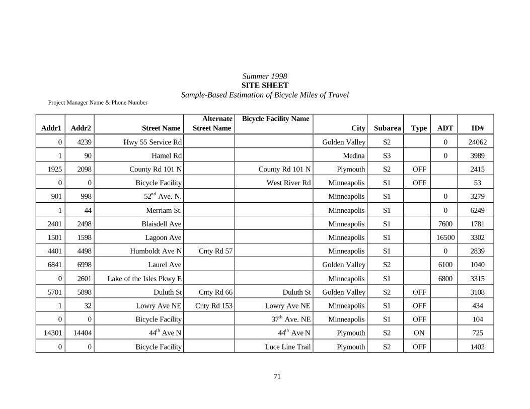
71

Summer 1998 SITE SHEET

Sample-Based Estimation of Bicycle Miles of Travel Project Manager Name & Phone Number

Addr1

Addr2

Street Name

Alternate Street Name

Bicycle Facility Name City

Subarea

Type

ADT

ID#

0 4239 Hwy 55 Service Rd Golden Valley S2 0 24062

1 90 Hamel Rd Medina S3 0 3989

1925 2098 County Rd 101 N County Rd 101 N Plymouth S2 OFF 2415

0 0 Bicycle Facility West River Rd Minneapolis S1 OFF 53

901 998 52nd Ave. N. Minneapolis S1 0 3279

1 44 Merriam St. Minneapolis S1 0 6249

2401 2498 Blaisdell Ave Minneapolis S1 7600 1781

1501 1598 Lagoon Ave Minneapolis S1 16500 3302

4401 4498 Humboldt Ave N Cnty Rd 57 Minneapolis S1 0 2839

6841 6998 Laurel Ave Golden Valley S2 6100 1040

0 2601 Lake of the Isles Pkwy E Minneapolis S1 6800 3315

5701 5898 Duluth St Cnty Rd 66 Duluth St Golden Valley S2 OFF 3108

1 32 Lowry Ave NE Cnty Rd 153 Lowry Ave NE Minneapolis S1 OFF 434

0 0 Bicycle Facility 37th Ave. NE Minneapolis S1 OFF 104

14301 14404 44th Ave N 44th Ave N Plymouth S2 ON 725

0 0 Bicycle Facility Luce Line Trail Plymouth S2 OFF 1402

72

Sample Based Estimation of Bicycle Miles of TravelUniversity of Minnesota

Department of Civil Engineering

Mpls

24062

3989

2415

53

3279

6249

1781

3302

2839

1040

3315

3108

434

104725

1402HIGHWAY 55

HIGHWAY 12

UN

IVER

SIT

Y A

VE

NEHIGHW

AY 55

HIG

HW

AY

169

HIGHW

AY 100

I 394

I 94

I 494

I 494

I 94I 394

I 35W

Golden Valley, Plymouth & N. Minneapolis Sites

General Site Map

73

24062

1040

3108

HIGHWAY 55H

IGH

WA

Y 1

00

GLENWOOD AVE

LAUREL AVE

DO

UG

LAS

DR

N

DULUTH ST

GOLDEN VALLEY RD

TH

EO

DO

RE

WIR

TH

PK

WY

COUNTRY CLUB DR

WESTERN AVE TU

RN

ER

S X

RD

S

RE

GE

NT

AV

E N

BR

UN

SW

ICK

AV

E N

AD

AIR

AV

E N

ME

ADO

W L

N

AR

DM

OR

E

LOU

ISIA

NA

AV

E

JER

SE

Y

Golden Valley Sites

Sample Based Estimation of Bicycle Miles of TravelUniversity of Minnesota

Department of Civil Engineering Detailed Site Map

74

B-6. Installation Sheet

Installation sheets, shown on the next page, are filled out in the field to keep track of

when and which cameras were installed at each site.

75

Summer 1998 EQUIPMENT INSTALLATION RECORD

Sample-Based Estimation of Bicycle Miles of Travel Project Manager Name & Phone Number

Date Time

TAPE#

IN

OUT

ON

OFF CAM

#

LOCATION

CITY SUB

AREA

TYPE*

ID#

* Type = ON OFF <5000 ≥5000

76

B-7. Count Sheet

An example of the sheet used to keep track of the counts taken from videotape is found

on the next page. Research assistants found it convenient and more accurate to stop every fifteen

minutes to record the count. It was also simple to record the weather seen during the fifteen-

minute count period. Both of these additional recordings can provide information beyond BMT,

regarding daily fluctuations and weather on bicycle use.

77

Subarea Type* ID#

Summer 1998 BICYCLE COUNT WORKSHEET

Sample-Based Estimation of Bicycle Miles of Travel

Count Date Jurisdiction Include Day Location

Start Time End Time Tape #

Counted By Total Note when darkness occurs in margin

Interval Weather Interval Weather Date Begin End Count Notes Date Begin End Count Notes

05:30 :45 13:30 :45 :45 6:00 :45 2:00 06:00 :15 14:00 :15 :15 :30 :15 :30 :30 :45 :30 :45 :45 7:00 :45 3:00 07:00 :15 15:00 :15 :15 :30 :15 :30 :30 :45 :30 :45 :45 8:00 :45 4:00 08:00 :15 16:00 :15 :15 :30 :15 :30 :30 :45 :30 :45 :45 9:00 :45 5:00 09:00 :15 17:00 :15 :15 :30 :15 :30 :30 :45 :30 :45 :45 10:00 :45 6:00 10:00 :15 18:00 :15 :15 :30 :15 :30 :30 :45 :30 :45 :45 11:00 :45 7:00 11:00 :15 19:00 :15 :15 :30 :15 :30 :30 :45 :30 :45 :45 12:00 :45 8:00 12:00 :15 20:00 :15 :15 :30 :15 :30 :30 :45 :30 :45 :45 P 1:00 :45 9:00 13:00 :15 21:00 :15 :15 :30 :15 :30

*Type = On; Off; <5000; or if >5000, record actual ADT

79

Appendix C POWER COMPANY REQUIREMENTS

81

Appendix D PROTECTION OF HUMAN SUBJECTS

82

The observation of public behavior is regulated by federal policy. Failure to obtain

permission to observe human behavior as part of a research project can terminate the research

even if all data is collected. The BMT project found that our methods fell within acceptable

policy guidelines as described in section 3.6.4.

The following is University of Minnesota policy:

University of Minnesota and federal policies require that research involving human subjects be reviewed to take into consideration:

1.The rights and welfare of the individual(s);

2.The appropriateness of the method(s); and

3.The balance of risks and potential benefits of the investigation.

These websites are recommended for understanding federal policy regarding human

subjects and the observation of public behavior.

Research Subject Protection Program http://www.research.umn.edu/subjects/index Protecting Human Subjects Guide: How to Apply for Review http://www.research.umn.edu/subjects/humans/guide/humans3 Office of Human Subjects Research at the National Institutes of Health http://ohsr.od.nih.gov

83

Appendix E BICYCLE COUNTS AND LOCATIONS

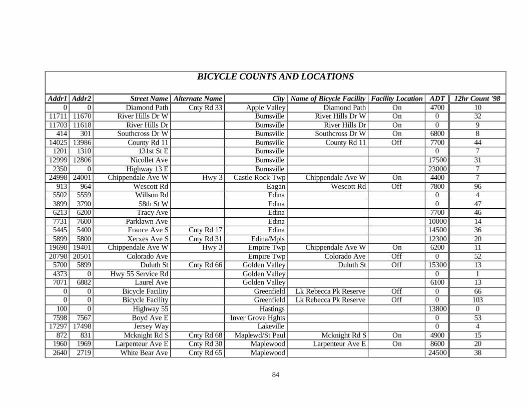
84

BICYCLE COUNTS AND LOCATIONS

Addr1 Addr2 Street Name Alternate Name City Name of Bicycle Facility Facility Location ADT 12hr Count '98 0 0 Diamond Path Cnty Rd 33 Apple Valley Diamond Path On 4700 10

11711 11670 River Hills Dr W Burnsville River Hills Dr W On 0 32 11703 11618 River Hills Dr Burnsville River Hills Dr On 0 9

414 301 Southcross Dr W Burnsville Southcross Dr W On 6800 8 14025 13986 County Rd 11 Burnsville County Rd 11 Off 7700 44

1201 1310 131st St E Burnsville 0 7 12999 12806 Nicollet Ave Burnsville 17500 31

2350 0 Highway 13 E Burnsville 23000 7 24998 24001 Chippendale Ave W Hwy 3 Castle Rock Twp Chippendale Ave W On 4400 7

913 964 Wescott Rd Eagan Wescott Rd Off 7800 96 5502 5559 Willson Rd Edina 0 4 3899 3790 58th St W Edina 0 47 6213 6200 Tracy Ave Edina 7700 46 7731 7600 Parklawn Ave Edina 10000 14 5445 5400 France Ave S Cnty Rd 17 Edina 14500 36 5899 5800 Xerxes Ave S Cnty Rd 31 Edina/Mpls 12300 20

19698 19401 Chippendale Ave W Hwy 3 Empire Twp Chippendale Ave W On 6200 11 20798 20501 Colorado Ave Empire Twp Colorado Ave Off 0 52

5700 5899 Duluth St Cnty Rd 66 Golden Valley Duluth St Off 15300 13 4373 0 Hwy 55 Service Rd Golden Valley 0 1 7071 6882 Laurel Ave Golden Valley 6100 13

0 0 Bicycle Facility Greenfield Lk Rebecca Pk Reserve Off 0 66 0 0 Bicycle Facility Greenfield Lk Rebecca Pk Reserve Off 0 103

100 0 Highway 55 Hastings 13800 0 7598 7567 Boyd Ave E Inver Grove Hghts 0 53

17297 17498 Jersey Way Lakeville 0 4 872 831 Mcknight Rd S Cnty Rd 68 Maplewd/St Paul Mcknight Rd S On 4900 15

1960 1969 Larpenteur Ave E Cnty Rd 30 Maplewood Larpenteur Ave E On 8600 20 2640 2719 White Bear Ave Cnty Rd 65 Maplewood 24500 38

85

BICYCLE COUNTS AND LOCATIONS

Addr1 Addr2 Street Name Alternate Name City Name of Bicycle Facility Facility Location ADT 12hr Count '98 0 0 Bicycle Facility Medina Baker Pk Reserve Off 0 21 0 0 Bicycle Facility Medina Baker Pk Reserve Off 0 171 0 0 Bicycle Facility Medina Baker Pk Reserve Off 0 233

4368 4399 Willow Dr Medina 0 2 3500 4099 Arrowhead Dr Medina 0 0 1999 1800 Ridge Dr S Medina 0 0 945 840 Foxberry Farms Rd Medina 0 17 73 2 Hamel Rd Medina 0 1

1600 2099 Highway 55 Medina 15800 7 800 1199 Olson Memorial Hwy Hwy 55 Medina 17700 2

2582 2551 Delaware Ave Cnty Rd 63 Mendota Heights 2900 33 1199 1100 5th St Se Minneapolis 5th St Se On 0 419 1098 1001 2nd St S Minneapolis 2nd St S On 0 143 899 800 5th St Se Minneapolis 5th St Se On 0 467 673 698 10th St S Minneapolis 10th St S On 0 72 200 299 Harvard St Se Minneapolis Harvard St Se On 0 154 599 500 20th Ave S Minneapolis 20th Ave S On 5600 452

4399 4300 Minnehaha Ave Cnty Rd 48 Minneapolis Minnehaha Ave On 6700 47 1799 1700 Park Ave Cnty Rd 33 Minneapolis Park Ave On 9500 193 401 498 10th St S Minneapolis 10th St S On 9600 131 960 999 15th Ave Se Minneapolis 15th Ave Se On 9800 1054 398 301 4th St S Minneapolis 4th St S On 10100 56

4067 4000 Minnehaha Ave Cnty Rd 48 Minneapolis Minnehaha Ave On 10200 35 499 400 University Ave Se Minneapolis University Ave Se On 12600 153 851 800 University Ave Se Minneapolis University Ave Se On 15300 401 600 699 15th Ave Se Minneapolis 15th Ave Se On 15300 968

1599 1500 University Ave Se Cnty Rd 36 Minneapolis University Ave Se On 16500 468 1699 1600 4th St Se Cnty Rd 37 Minneapolis 4th St Se On 19500 193 999 960 University Ave Se Cnty Rd 36 Minneapolis University Ave Se On 21500 801

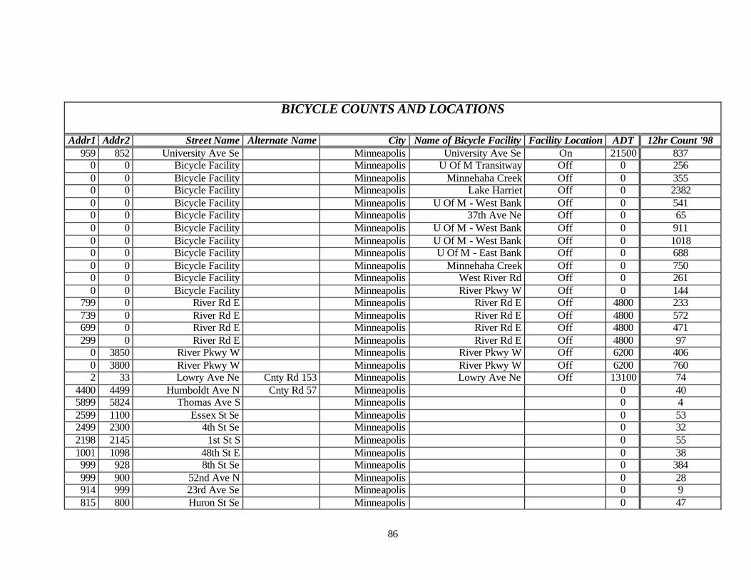
86

BICYCLE COUNTS AND LOCATIONS

Addr1 Addr2 Street Name Alternate Name City Name of Bicycle Facility Facility Location ADT 12hr Count '98 959 852 University Ave Se Minneapolis University Ave Se On 21500 837

0 0 Bicycle Facility Minneapolis U Of M Transitway Off 0 256 0 0 Bicycle Facility Minneapolis Minnehaha Creek Off 0 355 0 0 Bicycle Facility Minneapolis Lake Harriet Off 0 2382 0 0 Bicycle Facility Minneapolis U Of M - West Bank Off 0 541 0 0 Bicycle Facility Minneapolis 37th Ave Ne Off 0 65 0 0 Bicycle Facility Minneapolis U Of M - West Bank Off 0 911 0 0 Bicycle Facility Minneapolis U Of M - West Bank Off 0 1018 0 0 Bicycle Facility Minneapolis U Of M - East Bank Off 0 688 0 0 Bicycle Facility Minneapolis Minnehaha Creek Off 0 750 0 0 Bicycle Facility Minneapolis West River Rd Off 0 261 0 0 Bicycle Facility Minneapolis River Pkwy W Off 0 144

799 0 River Rd E Minneapolis River Rd E Off 4800 233 739 0 River Rd E Minneapolis River Rd E Off 4800 572 699 0 River Rd E Minneapolis River Rd E Off 4800 471 299 0 River Rd E Minneapolis River Rd E Off 4800 97

0 3850 River Pkwy W Minneapolis River Pkwy W Off 6200 406 0 3800 River Pkwy W Minneapolis River Pkwy W Off 6200 760 2 33 Lowry Ave Ne Cnty Rd 153 Minneapolis Lowry Ave Ne Off 13100 74

4400 4499 Humboldt Ave N Cnty Rd 57 Minneapolis 0 40 5899 5824 Thomas Ave S Minneapolis 0 4 2599 1100 Essex St Se Minneapolis 0 53 2499 2300 4th St Se Minneapolis 0 32 2198 2145 1st St S Minneapolis 0 55 1001 1098 48th St E Minneapolis 0 38 999 928 8th St Se Minneapolis 0 384 999 900 52nd Ave N Minneapolis 0 28 914 999 23rd Ave Se Minneapolis 0 9 815 800 Huron St Se Minneapolis 0 47

87

BICYCLE COUNTS AND LOCATIONS

Addr1 Addr2 Street Name Alternate Name City Name of Bicycle Facility Facility Location ADT 12hr Count '98 700 799 9th Ave Se Minneapolis 0 54 698 601 Godward St Ne Minneapolis 0 8 599 500 7th Ave Se Minneapolis 0 93 500 0 9th Ave Se Minneapolis 0 86 499 450 21st Ave S Minneapolis 0 374 199 100 2nd St Se Minneapolis 0 72 199 0 East River Rd Minneapolis 0 238 43 2 Merriam St Minneapolis 0 137 0 4850 Lake Harriet Pkwy W Minneapolis 4600 88

2901 2962 Stinson Blvd Cnty Rd 27 Minneapolis 6100 21 1299 1200 Como Ave Se Minneapolis 6300 212 3501 3598 42nd St E Minneapolis 6600 118 1000 1077 Fulton St Se Minneapolis 6600 57 800 899 Fulton St Se Minneapolis 6600 136 150 199 Pleasant St Se Minneapolis 6700 901

2667 0 Lk Of The Isles Pkwy E Minneapolis 6800 484 2499 2400 Blaisdell Ave Minneapolis 7600 132 3999 3900 Nicollet Ave Cnty Rd 52 Minneapolis 9500 63 2117 2000 University Ave Se Cnty Rd 36 Minneapolis 9800 116 784 799 10th Ave Se Minneapolis 10300 69

1000 1029 Washington Ave Se Hwy 122 Minneapolis 11000 163 900 999 Washington Ave Se Hwy 122 Minneapolis 11000 469 427 400 19th Ave S Minneapolis 13000 399

0 0 20th Ave S Minneapolis 15400 256 1801 1824 Central Ave Ne Hwy 65 Minneapolis 16000 98 1500 1599 Lagoon Ave Minneapolis 16500 120 1099 1000 4th St Se Cnty Rd 37 Minneapolis 20000 411 8399 8130 County Rd 110 W Minnetrista County Rd 110 W On 0 6 4238 4201 County Rd 44 Minnetrista County Rd 44 On 0 6

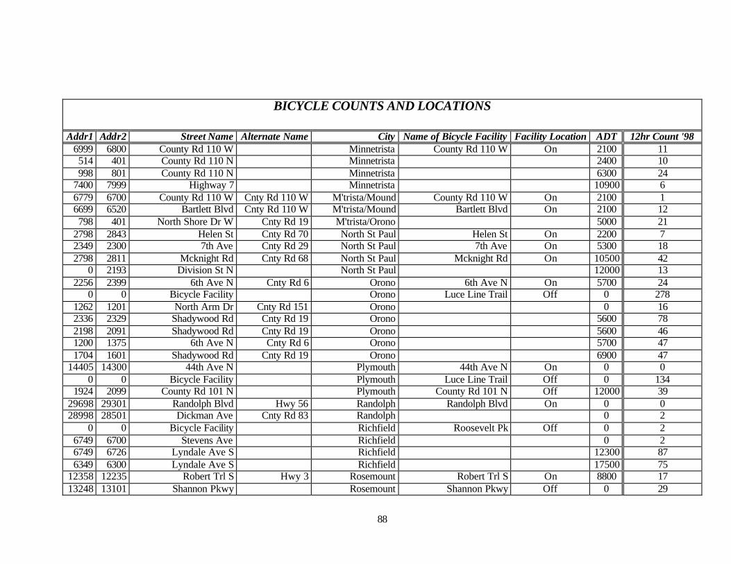
88

BICYCLE COUNTS AND LOCATIONS

Addr1 Addr2 Street Name Alternate Name City Name of Bicycle Facility Facility Location ADT 12hr Count '98 6999 6800 County Rd 110 W Minnetrista County Rd 110 W On 2100 11 514 401 County Rd 110 N Minnetrista 2400 10 998 801 County Rd 110 N Minnetrista 6300 24

7400 7999 Highway 7 Minnetrista 10900 6 6779 6700 County Rd 110 W Cnty Rd 110 W M'trista/Mound County Rd 110 W On 2100 1 6699 6520 Bartlett Blvd Cnty Rd 110 W M'trista/Mound Bartlett Blvd On 2100 12 798 401 North Shore Dr W Cnty Rd 19 M'trista/Orono 5000 21

2798 2843 Helen St Cnty Rd 70 North St Paul Helen St On 2200 7 2349 2300 7th Ave Cnty Rd 29 North St Paul 7th Ave On 5300 18 2798 2811 Mcknight Rd Cnty Rd 68 North St Paul Mcknight Rd On 10500 42

0 2193 Division St N North St Paul 12000 13 2256 2399 6th Ave N Cnty Rd 6 Orono 6th Ave N On 5700 24

0 0 Bicycle Facility Orono Luce Line Trail Off 0 278 1262 1201 North Arm Dr Cnty Rd 151 Orono 0 16 2336 2329 Shadywood Rd Cnty Rd 19 Orono 5600 78 2198 2091 Shadywood Rd Cnty Rd 19 Orono 5600 46 1200 1375 6th Ave N Cnty Rd 6 Orono 5700 47 1704 1601 Shadywood Rd Cnty Rd 19 Orono 6900 47

14405 14300 44th Ave N Plymouth 44th Ave N On 0 0 0 0 Bicycle Facility Plymouth Luce Line Trail Off 0 134

1924 2099 County Rd 101 N Plymouth County Rd 101 N Off 12000 39 29698 29301 Randolph Blvd Hwy 56 Randolph Randolph Blvd On 0 0 28998 28501 Dickman Ave Cnty Rd 83 Randolph 0 2

0 0 Bicycle Facility Richfield Roosevelt Pk Off 0 2 6749 6700 Stevens Ave Richfield 0 2 6749 6726 Lyndale Ave S Richfield 12300 87 6349 6300 Lyndale Ave S Richfield 17500 75

12358 12235 Robert Trl S Hwy 3 Rosemount Robert Trl S On 8800 17 13248 13101 Shannon Pkwy Rosemount Shannon Pkwy Off 0 29

89

BICYCLE COUNTS AND LOCATIONS

Addr1 Addr2 Street Name Alternate Name City Name of Bicycle Facility Facility Location ADT 12hr Count '98 0 0 Shannon Pkwy Rosemount Shannon Pkwy Off 3450 80

3998 3501 150th St W Cnty Rd 42 Rosemount 150th St W Off 20000 67 4384 4355 Upper 145th St W Rosemount 0 14 2888 2915 Rice St Hwy 49 Rosev/Lit.Canada 16000 63

0 0 Bicycle Facility Roseville Bennett Lk Off 0 19 2400 2535 Fairview Ave N Cnty Rd 48 Roseville Fairview Ave N Off 15000 39 1478 1459 Commerce St Roseville 0 4 651 678 Mound Ave Shoreview Mound Ave Off 0 59

1024 725 County Rd I W Cnty Rd 3 Shoreview County Rd I W Off 5400 37 244 233 Nichols Ct Shoreview 0 21

0 0 Bicycle Facility South St Paul S St Paul River Trail Off 0 11 3730 3809 Edgerton St Vadnais Heights Edgerton St On 2350 30

0 0 Bicycle Facility Vadnais Heights Lk Vadnais Off 0 128 701 624 Hiawatha Ave Vadnais Heights 0 14

16998 16501 Emery Ave Vermillion Twp 0 0

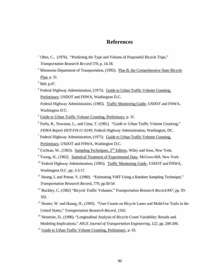
90

References 1 Ohrn, C., (1976). “Predicting the Type and Volume of Purposeful Bicycle Trips,”

Transportation Research Record 570, p. 14-18. 2 Minnesota Department of Transportation, (1992). Plan B, the Comprehensive State Bicycle

Plan, p. 31. 3 Ibid. p.47. 4 Federal Highway Administration, (1975). Guide to Urban Traffic Volume Counting,

Preliminary, USDOT and FHWA, Washington D.C.

Federal Highway Administration, (1985). Traffic Monitoring Guide, USDOT and FHWA,

Washington D.C. 5 Guide to Urban Traffic Volume Counting, Preliminary, p. 31. 6 Ferlis, R., Nowman, L., and Cima, T. (1981). “Guide to Urban Traffic Volume Counting,”

FHWA Report DOT-FH-11-9249, Federal Highway Administration, Washington, DC. 7 Federal Highway Administration, (1975). Guide to Urban Traffic Volume Counting,

Preliminary, USDOT and FHWA, Washington D.C. 8 Cochran, W., (1963). Sampling Techniques, 2nd Edition, Wiley and Sons, New York. 9 Young, H., (1962). Statistical Treatment of Experimental Data, McGraw-Hill, New York. 10 Federal Highway Administration, (1985). Traffic Monitoring Guide , USDOT and FHWA,

Washington D.C. pp. 3-3-17. 11 Hoang, L and Poteat, V, (1980). “Estimating VMT Using a Random Sampling Technique,”

Transportation Research Record, 779, pp.50-54 12 Buckley, C. (1982) “Bicycle Traffic Volumes,” Transportation Research Record 847, pp. 93-

102. 13 Hunter, W. and Huang, H., (1995). “User Counts on Bicycle Lanes and Multi-Use Trails in the

United States,” Transportation Research Record, 1502. 14 Neimeier, D., (1996). “Longitudinal Analysis of Bicycle Count Variability: Results and

Modeling Implications,” ASCE Journal of Transportation Engineering, 122, pp. 200-206. 15 Guide to Urban Traffic Volume Counting, Preliminary, p. 43.

91

16 Federal Highway Administration, (1975). Guide to Urban Traffic Volume Counting,

Preliminary, USDOT and FHWA, Washington D.C. 17 This area of the University of Minnesota has been the subject of a number of surveys and

counts on bicycle use, all indicating high bicycle use compared to non-University areas of the

region. One 2-day, ad-hoc, bicycle count taken in the fall of 1994 in the heart of the University

of Minnesota’s largest campus (East Bank in Minneapolis) showed that on the measured days,

10-21% of all vehicles on the count streets were bicycles. The data for this count is reported in

The University of Minnesota Bicycle Transportation Plan, 1996 18 Ibid, p. 32. 19 Ibid, p. 34. 20 Reference in Guide to Urban Traffic Volume Counting, Preliminary as follows:

Crow, Edwin L., Davis, Francis A., and Maxfield, Margaret, (1960). Statistics Manual, Dover

Publications Inc., New York. See Chart IX, p. 277. 21 Reference in Guide to Urban Traffic Volume Counting, Preliminary as follows:

Sampford, M.R., (1962). An Introduction to Sampling Theory, Oliver and Boyd, Edinburgh, p.

6-14. 22 Guide to Urban Traffic Volume Counting, Preliminary, p. 41. 23 American Association of State and Highway and Transportation Officials (AASHTO) Task

Force on Geometric Design (1991). Guide for the Development of Bicycle Facilities,

AASHTO, Washington D.C.

Federal Highway Administration, (1985). Selecting Roadway Design Treatments to

Accommodate Bicycles, (FHWA-RD-92-073), USDOT and FHWA, Washington D.C.

Federal Highway Administration, (1992). “Case Study No. 24: Current Planning Guidelines

and Design Standards Being Used By State and Local Agencies for Bicycle and Pedestrian

Facilities,” National Bicycle and Walking Study, (FHWA-PD-93-006), USDOT and FHWA,

Washington, D.C. 24 Sykes, Robert D. and Wicklatz Trina (1996). Creating Bicycle Transportation Networks: A

Guidebook, Minnesota Department of Transportation, St. Paul, MN. 25 Sustainable Transportation Initiative Unit, Minnesota Department of Transportation (1997).

“Data from the 1996 Minnesota Bicycle Miles Traveled (BMT) Project,” Office Memorandum,

Sustainable Transportation Initiatives Group, Mn/DOT.

92

26 Ibid. 27 DOQs are aerial photographs that have been adjusted to account for the curvature of the earth.

DOQs make it possible to accurately scale (measure length on) aerial photographs. In other

words, DOQs are like maps because a measurement taken on a DOQ will equal the same

measurement taken on a map of the same scale. This is not true of aerial photographs. 28 Cochran, William G., (1977). Sampling Techniques, 3rd edition, John Wiley and Sons, New

York. 29 Ibid.