©2003 thomson/south-western 1 chapter 19 – decision making under uncertainty slides prepared by...
TRANSCRIPT
©2003 Thomson/South-Western 1
Chapter 19 –Chapter 19 –
Decision Decision Making Under Making Under UncertaintyUncertainty
Slides prepared by Jeff Heyl, Lincoln UniversitySlides prepared by Jeff Heyl, Lincoln University©2003 South-Western/Thomson Learning™
Introduction toIntroduction to Business StatisticsBusiness Statistics, 6e, 6eKvanli, Pavur, KeelingKvanli, Pavur, Keeling

©2003 Thomson/South-Western 2
Two Basic QuestionsTwo Basic Questions
What are the possible actions What are the possible actions (alternatives) for this problem?(alternatives) for this problem?
What is it about the future that What is it about the future that affects the desirability of each affects the desirability of each action?action?
©2003 Thomson/South-Western 3
TermsTerms Descriptions of the future: states of Descriptions of the future: states of
naturenature The state of nature items are outcomes.The state of nature items are outcomes.
The key distinction between an action and a The key distinction between an action and a state of nature is that the action is taken is state of nature is that the action is taken is under your control, whereas the state of under your control, whereas the state of nature that occurs is strictly a matter of nature that occurs is strictly a matter of chance.chance.
The payoff is the result of an action (A) an The payoff is the result of an action (A) an a state of nature (S)a state of nature (S)

©2003 Thomson/South-Western 4
Payoff TablePayoff Table
States of NatureStates of Nature
ActionAction SS11 SS22 SS33 …… SSnn
AA11 1111 1212 1313 …… 11nn
AA22 2121 2222 2323 …… 22nn
AA33 3131 3232 3333 …… 33nn
AAkk kk11 kk22 kk33 …… knkn
Table 19.1Table 19.1
©2003 Thomson/South-Western 5
Conservative (Minimax) Conservative (Minimax) StrategyStrategy
The action chosen is that action that The action chosen is that action that under the under the worstworst conditions produces the conditions produces the lowest “loss”lowest “loss”
The opportunity loss, LThe opportunity loss, Lijij, is the difference , is the difference
between the payoff for action I and the between the payoff for action I and the payoff for the action that would have the payoff for the action that would have the largest payoff under the state of nature jlargest payoff under the state of nature j

©2003 Thomson/South-Western 6
Minimax StrategyMinimax Strategy
Construct an opportunity loss table by Construct an opportunity loss table by using the maximum payoff for each state using the maximum payoff for each state of natureof nature
Determine the maximum opportunity loss Determine the maximum opportunity loss for each actionfor each action
Find the minimum value of the Find the minimum value of the opportunity losses found in step 2; the opportunity losses found in step 2; the corresponding action is the one selectedcorresponding action is the one selected

©2003 Thomson/South-Western 7
The Gambler (Maximax) The Gambler (Maximax) StrategyStrategy
The Maximax strategy is to choose The Maximax strategy is to choose that action having the largest that action having the largest
possible payoffpossible payoff

©2003 Thomson/South-Western 8
The Strategist The Strategist (Maximizing the Expected Payoff)(Maximizing the Expected Payoff)
This strategy assigns a probability to This strategy assigns a probability to each state of natureeach state of nature
The expected payoff of each action is The expected payoff of each action is determineddetermined
The action chosen is that action that The action chosen is that action that produces the largest expected payoffproduces the largest expected payoff

©2003 Thomson/South-Western 9
Sailtown ExampleSailtown Example
Average Interest RateAverage Interest Rate
Amount OrderedAmount Ordered Increases (Increases (SS11)) Steady (Steady (SS22)) Decreases (Decreases (SS33))
50 (50 (AA11)) 1515 1515 1515
75 (75 (AA22)) 2.52.5 22.522.5 22.522.5
100 (100 (AA33)) -10-10 3030 3030
150 (150 (AA44)) -35-35 55 4545
Table 19.1Table 19.1
©2003 Thomson/South-Western 10
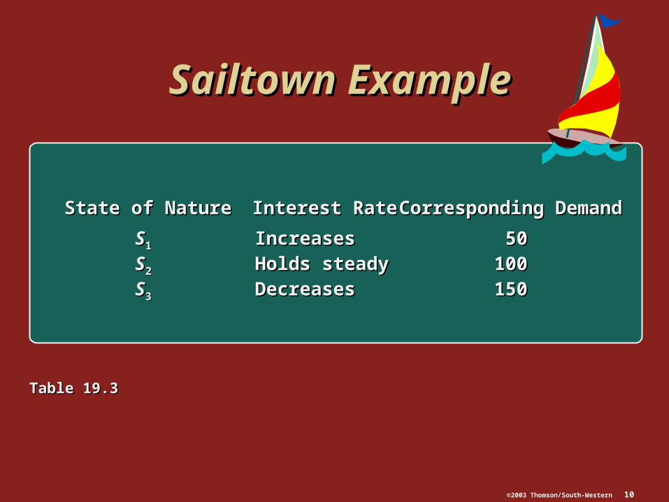
Sailtown ExampleSailtown Example
Table 19.3Table 19.3
State of NatureState of Nature Interest RateInterest Rate Corresponding DemandCorresponding Demand
SS11 IncreasesIncreases 5050
SS22 Holds steadyHolds steady 100100
SS33 DecreasesDecreases 150150

©2003 Thomson/South-Western 11
Sailtown ExampleSailtown Example
Revenue forRevenue for Loss Due toLoss Due toActionAction Boats SoldBoats Sold Returned BoatsReturned Boats Net PayoffNet Payoff
AA11 50 • $15,00050 • $15,000 0 • 5000 • 500 = $0= $0 $15,000$15,000
AA22 50 • $15,00050 • $15,000 25 • 50025 • 500 = $12,00= $12,00 $2.500$2.500
AA33 50 • $15,00050 • $15,000 50 • 50050 • 500 = $25,000= $25,000 -$10,000-$10,000
AA44 50 • $15,00050 • $15,000 100 • 500100 • 500 = $50,000= $50,000 -$35,000-$35,000
Table 19.4Table 19.4
©2003 Thomson/South-Western 12
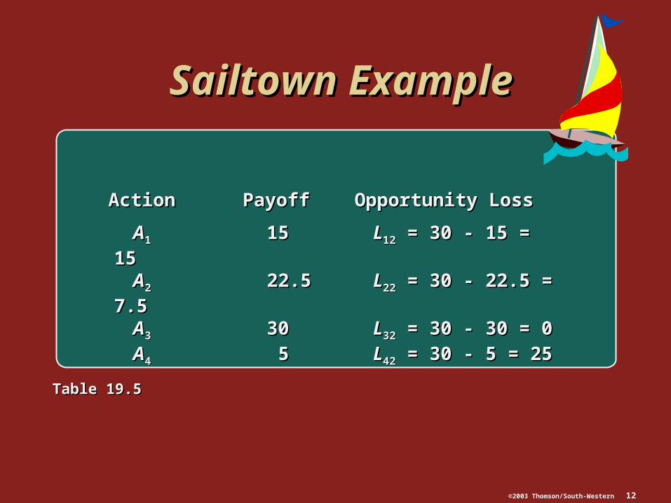
Sailtown ExampleSailtown Example
ActionAction PayoffPayoff Opportunity LossOpportunity Loss
AA11 1515 LL1212 = 30 - 15 = 15 = 30 - 15 = 15
AA22 22.522.5 LL2222 = 30 - 22.5 = 7.5 = 30 - 22.5 = 7.5
AA33 3030 LL3232 = 30 - 30 = 0 = 30 - 30 = 0
AA44 55 LL4242 = 30 - 5 = 25 = 30 - 5 = 25
Table 19.5Table 19.5

©2003 Thomson/South-Western 13
Sailtown ExampleSailtown Example
ActionAction PayoffPayoff Opportunity LossOpportunity Loss
AA11 1515 LL1212 = 45 - 15 = 30 = 45 - 15 = 30
AA22 22.522.5 LL2222 = 45 - 22.5 = 22.5 = 45 - 22.5 = 22.5
AA33 3030 LL3232 = 45 - 30 = 15 = 45 - 30 = 15
AA44 4545 LL4242 = 45 - 5 = 0 = 45 - 5 = 0
Table 19.6Table 19.6

©2003 Thomson/South-Western 14
Sailtown ExampleSailtown Example
Table 19.7Table 19.7
State of NatureState of Nature
ActionAction SS11 SS22 SS33
AA11 00 1515 3030
AA22 12.512.5 7.57.5 22.522.5
AA33 2525 00 1515
AA44 5050 2525 00

©2003 Thomson/South-Western 15
Sailtown ExampleSailtown Example
State of NatureState of Nature ProbabilityProbability
SS11: Interest rate increases: Interest rate increases PP((SS11) = .3) = .3
SS22: Interest rate remains unchanged: Interest rate remains unchanged PP((SS22) = .2) = .2
SS33: Interest rate decreases: Interest rate decreases PP((SS33) = .5) = .5
Table 19.10Table 19.10

©2003 Thomson/South-Western 16
Sailtown ExampleSailtown Example
ActionAction Expected PayoffExpected Payoff
AA11: Order 50 sailboats: Order 50 sailboats (15)(.3) + (15)(.2) + (15)(.5) = 15(15)(.3) + (15)(.2) + (15)(.5) = 15
AA22: Order 75 sailboats: Order 75 sailboats (2.5)(.3) + (22.5)(.2) + (22.5)(.5) = 16.5(2.5)(.3) + (22.5)(.2) + (22.5)(.5) = 16.5
AA33: Order 100 sailboats: Order 100 sailboats (-10)(.3) + (30)(.2) + (30)(.5) = 18(-10)(.3) + (30)(.2) + (30)(.5) = 18
AA44: Order 150 sailboats: Order 150 sailboats (-35)(.3) + (5)(.2) + (45)(.5) = 13(-35)(.3) + (5)(.2) + (45)(.5) = 13
Table 19.11Table 19.11

©2003 Thomson/South-Western 17
Sailtown ExampleSailtown Example
Table 19.16Table 19.16
Expected PayoffExpected Payoff
PP((SS11)) PP((SS22)) PP((SS33)) AA11 AA22 AA33 AA44
.4.4 .2.2 .4.4 1515 14.514.5 1414 55
.4.4 .3.3 .3.3 1515 14.514.5 1414 11
.4.4 .1.1 .5.5 1515 14.514.5 1414 99
.5.5 .2.2 .3.3 1515 12.512.5 1010 -3-3
.5.5 .1.1 .4.4 1515 12.512.5 1010 11
.3.3 .3.3 .4.4 1515 16.516.5 1818 99
.3.3 .2.2 .5.5 1515 16.516.5 1818 1313
©2003 Thomson/South-Western 18
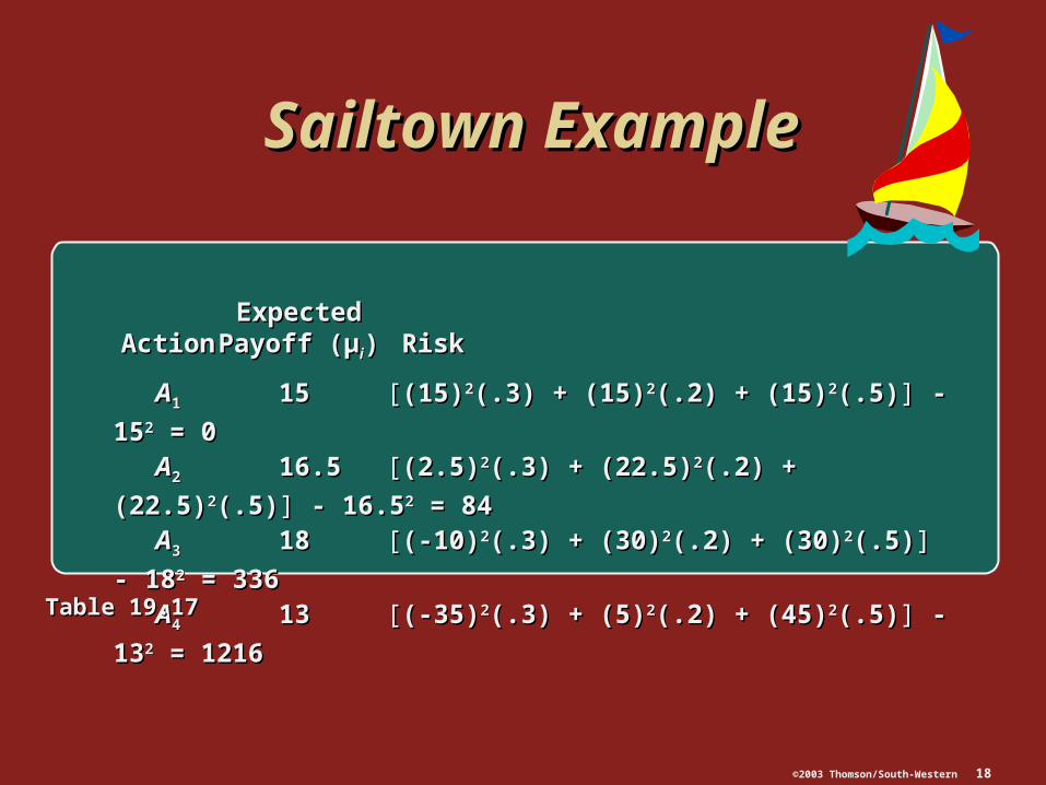
Sailtown ExampleSailtown Example
ExpectedExpectedActionAction Payoff (µPayoff (µii)) Risk Risk
AA11 1515 [[(15)(15)22(.3) + (15)(.3) + (15)22(.2) + (15)(.2) + (15)22(.5)(.5)]] - 15 - 1522 = 0 = 0
AA22 16.516.5 [[(2.5)(2.5)22(.3) + (22.5)(.3) + (22.5)22(.2) + (22.5)(.2) + (22.5)22(.5)(.5)]] - 16.5 - 16.522 = 84 = 84
AA33 1818 [[(-10)(-10)22(.3) + (30)(.3) + (30)22(.2) + (30)(.2) + (30)22(.5)(.5)]] - 18 - 1822 = 336 = 336
AA44 1313 [[(-35)(-35)22(.3) + (5)(.3) + (5)22(.2) + (45)(.2) + (45)22(.5)(.5)]] - 13 - 1322 = 1216 = 1216
Table 19.17Table 19.17

©2003 Thomson/South-Western 19
Sailtown ExampleSailtown Example
Figure 18.1Figure 18.1

©2003 Thomson/South-Western 20
UtilityUtility
Utility combines the decision Utility combines the decision maker’s attitude toward the payoff maker’s attitude toward the payoff and the corresponding risk of each and the corresponding risk of each alternativealternative
The utility value of a particular The utility value of a particular outcome is used to measure both outcome is used to measure both the attractiveness and the risk the attractiveness and the risk associated with this dollar amountassociated with this dollar amount

©2003 Thomson/South-Western 21
Utility ValueUtility Value
Step 1: Assign a utility value of Step 1: Assign a utility value of 00 to to the smallest payoff amount (the smallest payoff amount (minmin ) and ) and
a value of a value of 100100 to the largest ( to the largest (maxmax ) )
Step 2: The utility value for any payoff Step 2: The utility value for any payoff under consideration is found by under consideration is found by using:U(using:U(ijij) = P ) = P * 100* 100

©2003 Thomson/South-Western 22
UtilityUtility
Utility of 11,200Utility of 11,200
Uti
lity
Uti
lity
100100
5050
00
|
11,20011,200
|
40,00040,000ProfitProfit
Figure 18.2Figure 18.2
©2003 Thomson/South-Western 23
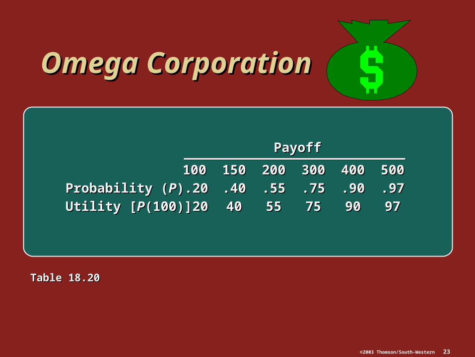
Omega CorporationOmega Corporation
PayoffPayoff
100100 150150 200200 300300 400400 500500
Probability (Probability (PP)) .20.20 .40.40 .55.55 .75.75 .90.90 .97.97
Utility [Utility [PP(100)](100)] 2020 4040 5555 7575 9090 9797
Table 18.20Table 18.20

©2003 Thomson/South-Western 24
Decision Trees Decision Trees and Bayes’ Ruleand Bayes’ Rule
A decision tree graphically represents A decision tree graphically represents the entire decision problem, including:the entire decision problem, including: The possible actions facing the decision The possible actions facing the decision
makermaker The outcomes that can occurThe outcomes that can occur The relationships between the actions The relationships between the actions
and outcomesand outcomes
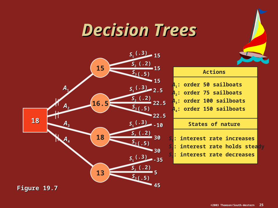
©2003 Thomson/South-Western 25
Decision TreesDecision Trees
1818
15
16.5
18
13
AA11
AA22
AA33
AA44
SS11
SS22
SS33
(.3)(.3)
(.2)(.2)
(.5)(.5)
SS11
SS22
SS33
(.3)(.3)
(.2)(.2)
(.5)(.5)
SS11
SS22
SS33
(.3)(.3)
(.2)(.2)
(.5)(.5)
SS11
SS22
SS33
(.3)(.3)
(.2)(.2)
(.5)(.5)
1515
1515
1515
2.52.5
22.522.5
22.522.5
-10-10
3030
3030
-35-35
55
4545
Actions
States of nature
A1: order 50 sailboats
A2: order 75 sailboats
A3: order 100 sailboats
A4: order 150 sailboats
S1: interest rate increases
S2: interest rate holds steady
S3: interest rate decreases
Figure 19.7Figure 19.7

©2003 Thomson/South-Western 26
Decision Trees Decision Trees and Bayes’ Ruleand Bayes’ Rule
Bayes’ rule allows you to revise a Bayes’ rule allows you to revise a probability in light of certain probability in light of certain information that is providedinformation that is provided
PP((EEii||BB) = =) = =PP((EEii and and BB))
PP((BB))
iith pathth path
sum of pathssum of paths

©2003 Thomson/South-Western 27
Use of Bayes’ RuleUse of Bayes’ Rule
AA11
AA22
AA33
AA44
SS11
SS22
SS33
SS11
SS22
SS33
SS11
SS22
SS33
SS11
SS22
SS33
1515
1515
1515
2.52.5
22.522.5
22.522.5
-10-10
3030
3030
-35-35
55
4545
Actions
States of nature
A1: order 50 sailboats
A2: order 75 sailboats
A3: order 100 sailboats
A4: order 150 sailboats
S1: interest rate increases
S2: interest rate holds steady
S3: interest rate decreases
Figure 19.8Figure 19.8

©2003 Thomson/South-Western 28
Deriving the Posterior Deriving the Posterior ProbabilitiesProbabilities
Consultant predicts an increase (Consultant predicts an increase (II11))
Consultant predicts an increase (Consultant predicts an increase (II11))
Consultant predicts an increase (Consultant predicts an increase (II11))
.7.7
.4.4
.2.2
SS11
SS22
SS33
(.3)(.3)
(.2)(.2)
(.5)(.5)
Figure 19.9Figure 19.9

©2003 Thomson/South-Western 29
Resulting Decision TreeResulting Decision Tree
AA11
AA22
AA33
AA44
SS11
SS22
SS33
(.538)(.538)
(.205)(.205)
(.256)(.256)
(.538)(.538)
(.205)(.205)
(.256)(.256)
(.538)(.538)
(.205)(.205)
(.256)(.256)
(.538)(.538)
(.205)(.205)
(.256)(.256)
1515
1515
1515
2.52.5
22.522.5
22.522.5
-10-10
3030
3030-35-35
55
4545
SS11
SS22
SS33
SS11
SS22
SS33
SS11
SS22
SS33
15
8.45
-6.28
11.72
Consultant predictsConsultant predicts
an increase (an increase (II11))1818
Figure 19.10Figure 19.10

©2003 Thomson/South-Western 30
Completed Completed Decision Decision Tree for Tree for Sailtown Sailtown ProblemProblem
Figure 19.11Figure 19.11
AA11
AA22
AA33
AA44
SS11
SS22
SS33
(.3)(.3)
(.2)(.2)
(.5)(.5)
1515
1515
1515SS11
SS22
SS33
(.3)(.3)
(.2)(.2)
(.5)(.5)
2.52.5
22.522.5
22.522.5SS11
SS22
SS33
(.3)(.3)
(.2)(.2)
(.5)(.5)
-10-10
3030
3030SS11
SS22
SS33
(.3)(.3)
(.2)(.2)
(.5)(.5)
-35-35
55
4545
21.321.3
15
13
16.5
18
AA11
AA22
AA33
AA44
SS11
SS22
SS33
(.538)(.538)
(.205)(.205)
(.256)(.256)
1515
1515
15152.52.5
22.522.5
22.522.5-10-10
3030
3030-35-35
55
4545
1515
15
SS11
SS22
SS33
(.538)(.538)
(.205)(.205)
(.256)(.256)-6.28
SS11
SS22
SS33
(.538)(.538)
(.205)(.205)
(.256)(.256)
SS11
SS22
SS33
(.538)(.538)
(.205)(.205)
(.256)(.256)
11.72
8.45
AA11
AA22
AA33
AA44
20.7920.79
SS11
SS22
SS33
(.231)(.231)
(.385)(.385)
(.385)(.385)
1515
1515
1515
15
SS11
SS22
SS33
(.231)(.231)
(.385)(.385)
(.385)(.385)
-35-35
55
4545
11.16
SS11
SS22
SS33
(.231)(.231)
(.385)(.385)
(.385)(.385)
2.52.5
22.522.5
22.522.517.90
SS11
SS22
SS33
(.231)(.231)
(.385)(.385)
(.385)(.385)
-10-10
3030
3030
20.79
AA11
AA22
AA33
AA44
SS11
SS22
SS33
(.086)(.086)
(.057)(.057)
(.857)(.857)
1515
1515
15152.52.5
22.522.5
22.522.5-10-10
3030
3030-35-35
55
4545
35.8435.84
15
SS11
SS22
SS33
(.086)(.086)
(.057)(.057)
(.857)(.857)35.84
SS11
SS22
SS33
(.086)(.086)
(.057)(.057)
(.857)(.857)
SS11
SS22
SS33
(.086)(.086)
(.057)(.057)
(.857)(.857)
20.78
26.56
23.80
-2.5
NoNoadditional additional informationinformation
PurchasePurchaseadditionaladditionalinformationinformation
II11
II22
II33
(.35)(.35)
(.26)(.26)
(.39)(.39)

©2003 Thomson/South-Western 31
Deriving the Posterior Deriving the Posterior ProbabilitiesProbabilities
SS11
SS33
SS22
(.3)(.3)
(.2)(.2)
(.5)(.5)
(.7)(.7)
(.4)(.4)
(.2)(.2)II11
II11
II11
AA
Sum of branchesSum of branches = = PP((II11))
= .39= .39PP((SS11 | | II11) = .21/.39) = .21/.39 = .538= .538
PP((SS22 | | II11) = .08/.39) = .08/.39 = .205= .205
PP((SS33 | | II11) = .10/.39) = .10/.39 = .256= .256
1.01.0
SS11
SS33
SS22
(.3)(.3)
(.2)(.2)
(.5)(.5)
(.2)(.2)
(.5)(.5)
(.2)(.2)II22
II22
II22
AA
Sum of branchesSum of branches = = PP((II22))
= .26= .26PP((SS11 | | II22) = .06/.26) = .06/.26 = .231= .231
PP((SS22 | | II22) = .10/.26) = .10/.26 = .385= .385
PP((SS33 | | II22) = .10/.26) = .10/.26 = .385= .385
1.01.0
SS11
SS33
SS22
(.3)(.3)
(.2)(.2)
(.5)(.5)
(.1)(.1)
(.1)(.1)
(.6)(.6)II33
II33
II33
AA
Sum of branchesSum of branches = = PP((II33))
= .35= .35PP((SS11 | | II33) = .03/.35) = .03/.35 = .086= .086
PP((SS22 | | II33) = .02/.35) = .02/.35 = .057= .057
PP((SS33 | | II33) = .30/.35) = .30/.35 = .857= .857
1.01.0
Figure 19.12Figure 19.12